Sparse Interpolation - University of Illinois at...

Sparse Interpolation

1 Prony’s Methodinterpolation for coefficients and exponents

2 Singularities of Stewart-Gough platformscomputing the determinant of the Jacobian matrix

3 Reformulating Prony’s Methodderiving a generalized eigenvalue problemthe QZ method to solve Ax = λBx

4 The qd Algorithmdetermining the size of the support

MCS 563 Lecture 29Analytic Symbolic ComputationJan Verschelde, 21 March 2014

Analytic Symbolic Computation (MCS 563) Sparse Interpolation L-29 21 March 2014 1 / 32

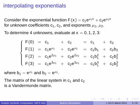
interpolating exponentials

Consider the exponential function F (x) = c1eµ1x + c2eµ2x

for unknown coefficients c1, c2, and exponents µ1, µ2.

To determine 4 unknowns, evaluate at x = 0, 1, 2, 3:

F (0) = c1 + c2 = c1 + c2

F (1) = c1eµ1 + c2eµ2 = c1b1 + c2b2

F (2) = c1e2µ1 + c2e2µ2 = c1b21 + c2b2

2

F (3) = c1e3µ1 + c2e3µ2 = c1b31 + c2b3

2

where b1 = eµ1 and b2 = eµ2.

The matrix of the linear system in c1 and c2

is a Vandermonde matrix.


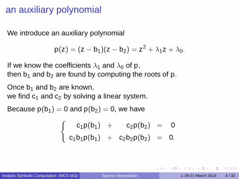
an auxiliary polynomial

We introduce an auxiliary polynomial

p(z) = (z − b1)(z − b2) = z2 + λ1z + λ0.

If we know the coefficients λ1 and λ0 of p,then b1 and b2 are found by computing the roots of p.

Once b1 and b2 are known,we find c1 and c2 by solving a linear system.

Because p(b1) = 0 and p(b2) = 0, we have{

c1p(b1) + c2p(b2) = 0

c1b1p(b1) + c2b2p(b2) = 0.


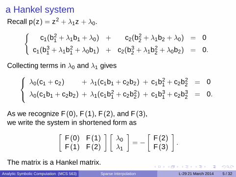
a Hankel systemRecall p(z) = z2 + λ1z + λ0.

{c1(b2

1 + λ1b1 + λ0) + c2(b22 + λ1b2 + λ0) = 0

c1(b31 + λ1b2

1 + λ0b1) + c2(b32 + λ1b2

2 + λ0b2) = 0.

Collecting terms in λ0 and λ1 gives

λ0(c1 + c2) + λ1(c1b1 + c2b2) + c1b21 + c2b2

2 = 0

λ0(c1b1 + c2b2) + λ1(c1b21 + c2b2

2) + c1b31 + c2b3

2 = 0.

As we recognize F (0), F (1), F (2), and F (3),we write the system in shortened form as

[F (0) F (1)F (1) F (2)

] [λ0

λ1

]= −

[F (2)F (3)

].

The matrix is a Hankel matrix.


the method of Prony

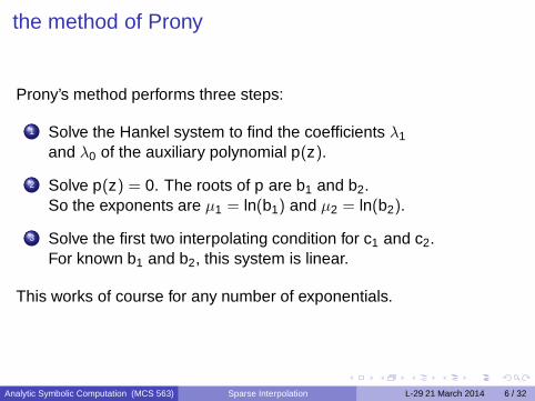
Prony’s method performs three steps:

1 Solve the Hankel system to find the coefficients λ1

and λ0 of the auxiliary polynomial p(z).

2 Solve p(z) = 0. The roots of p are b1 and b2.So the exponents are µ1 = ln(b1) and µ2 = ln(b2).

3 Solve the first two interpolating condition for c1 and c2.For known b1 and b2, this system is linear.

This works of course for any number of exponentials.


Stewart-Gough Platforms

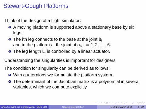
Think of the design of a flight simulator:

A moving platform is supported above a stationary base by sixlegs.

The i th leg connects to the base at the joint bi

and to the platform at the joint at ai , i = 1, 2, . . . , 6.

The leg length Li is controlled by a linear actuator.

Understanding the singularities is important for designers.

The condition for singularity can be derived as follows:

With quaternions we formulate the platform system.

The determinant of the Jacobian matrix is a polynomial in severalvariables, which we compute explicitly.


deriving equations

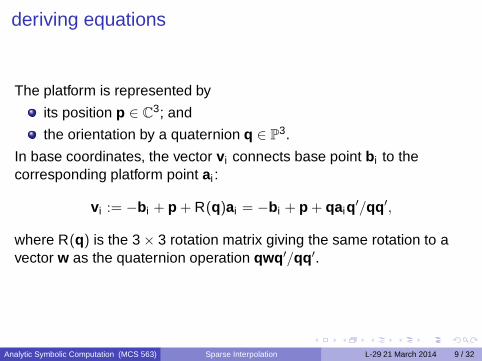
The platform is represented by

its position p ∈ C3; and

the orientation by a quaternion q ∈ P3.

In base coordinates, the vector vi connects base point bi to thecorresponding platform point ai :

vi := −bi + p + R(q)ai = −bi + p + qaiq′/qq′,

where R(q) is the 3 × 3 rotation matrix giving the same rotation to avector w as the quaternion operation qwq′/qq′.


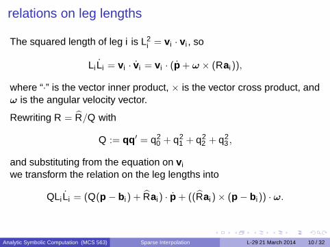
relations on leg lengths

The squared length of leg i is L2i = vi · vi , so

Li Li = vi · vi = vi · (p + ω × (Rai)),

where “·” is the vector inner product, × is the vector cross product, andω is the angular velocity vector.

Rewriting R = R/Q with

Q := qq′ = q20 + q2

1 + q22 + q2

3 ,

and substituting from the equation on vi

we transform the relation on the leg lengths into

QLi Li = (Q(p − bi) + Rai) · p + ((Rai) × (p − bi)) · ω.


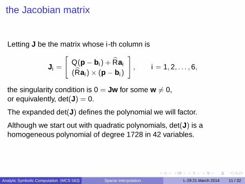
the Jacobian matrix

Letting J be the matrix whose i-th column is

Ji =

[Q(p − bi) + Rai

(Rai) × (p − bi)

]

, i = 1, 2, . . . , 6,

the singularity condition is 0 = Jw for some w 6= 0,or equivalently, det(J) = 0.

The expanded det(J) defines the polynomial we will factor.

Although we start out with quadratic polynomials, det(J) is ahomogeneous polynomial of degree 1728 in 42 variables.


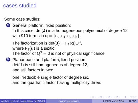
cases studied

Some case studies:1 General platform, fixed position:

In this case, det(J) is a homogeneous polynomial of degree 12with 910 terms in q = {q0, q1, q2, q3}.

The factorization is det(J) = F1(q)Q3,where F1(q) is a sextic.The factor of Q3 = 0 is not of physical significance.

2 Planar base and platform, fixed position:det(J) is still homogeneous of degree 12,and still factors in two:

one irreducible single factor of degree six,and the quadratic factor having multiplicity three.


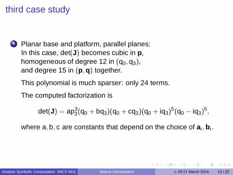
third case study

3 Planar base and platform, parallel planes:In this case, det(J) becomes cubic in p,homogeneous of degree 12 in (q0, q3),and degree 15 in (p, q) together.

This polynomial is much sparser: only 24 terms.

The computed factorization is

det(J) = ap33(q0 + bq3)(q0 + cq3)(q0 + iq3)

5(q0 − iq3)5,

where a, b, c are constants that depend on the choice of ai , bi .


numerical problems

The three steps in Prony’s algorithmall suffer numerical problems:

1 a Hankel matrix might be very ill-conditioned;2 the roots are often very sensitive to small changes

in the coefficients;3 Vandermonde matrices are also typically ill-conditioned.

Therefore, we reformulate the problem.


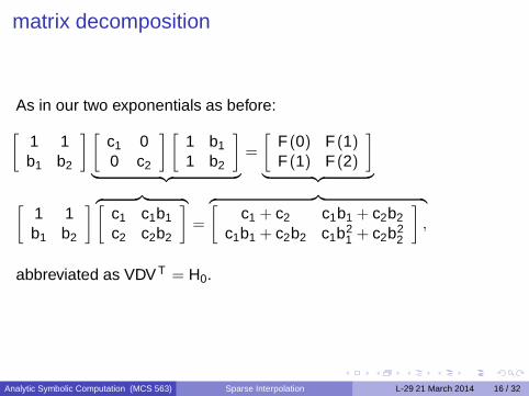
matrix decomposition

As in our two exponentials as before:

[1 1b1 b2

] [c1 00 c2

] [1 b1

1 b2

]

︸︷︷︸=

[F (0) F (1)F (1) F (2)

]

︸︷︷︸

[1 1b1 b2

] ︷︸︸︷[c1 c1b1

c2 c2b2

]=

︷︸︸︷[c1 + c2 c1b1 + c2b2

c1b1 + c2b2 c1b21 + c2b2

2

],

abbreviated as VDV T = H0.


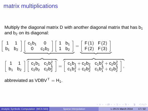
matrix multiplications

Multiply the diagonal matrix D with another diagonal matrix that has b1

and b2 on its diagonal:

[1 1b1 b2

] [c1b1 0

0 c2b2

] [1 b1

1 b2

]

︸︷︷︸=

[F (1) F (2)F (2) F (3)

]

︸︷︷︸

[1 1b1 b2

] ︷︸︸︷[c1b1 c1b2

1c2b2 c2b2

2

]=

︷︸︸︷[c1b1 + c2b2 c1b2

1 + c2b22

c1b21 + c2b2

2 c1b31 + c2b3

2

],

abbreviated as VDBV T = H1.


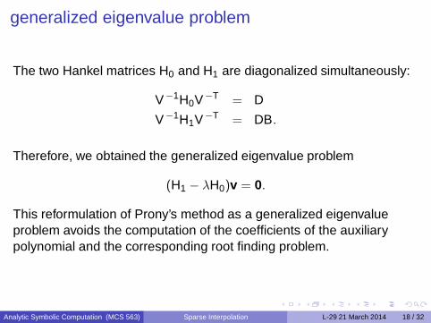
generalized eigenvalue problem

The two Hankel matrices H0 and H1 are diagonalized simultaneously:

V−1H0V−T = D

V−1H1V−T = DB.

Therefore, we obtained the generalized eigenvalue problem

(H1 − λH0)v = 0.

This reformulation of Prony’s method as a generalized eigenvalueproblem avoids the computation of the coefficients of the auxiliarypolynomial and the corresponding root finding problem.


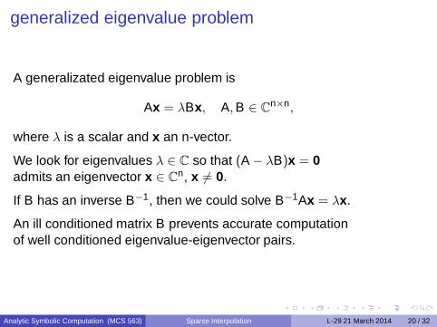
generalized eigenvalue problem

A generalizated eigenvalue problem is

Ax = λBx, A, B ∈ Cn×n,

where λ is a scalar and x an n-vector.

We look for eigenvalues λ ∈ C so that (A − λB)x = 0admits an eigenvector x ∈ C

n, x 6= 0.

If B has an inverse B−1, then we could solve B−1Ax = λx.

An ill conditioned matrix B prevents accurate computationof well conditioned eigenvalue-eigenvector pairs.


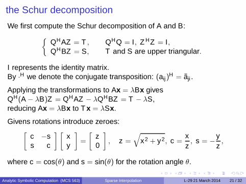
the Schur decomposition

We first compute the Schur decomposition of A and B:{

QHAZ = T ,

QHBZ = S,

QHQ = I, Z HZ = I,T and S are upper triangular.

I represents the identity matrix.By ·H we denote the conjugate transposition: (aij)

H = aji .

Applying the transformations to Ax = λBx givesQH(A − λB)Z = QHAZ − λQHBZ = T − λS,reducing Ax = λBx to T x = λSx.

Givens rotations introduce zeroes:[

c −ss c

] [xy

]=

[z0

], z =

√x2 + y2, c =

xz

, s = −yz

,

where c = cos(θ) and s = sin(θ) for the rotation angle θ.


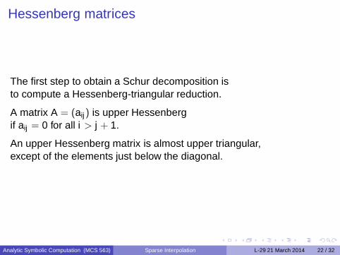
Hessenberg matrices

The first step to obtain a Schur decomposition isto compute a Hessenberg-triangular reduction.

A matrix A = (aij) is upper Hessenbergif aij = 0 for all i > j + 1.

An upper Hessenberg matrix is almost upper triangular,except of the elements just below the diagonal.


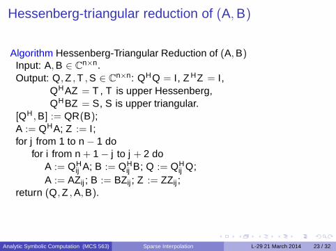
Hessenberg-triangular reduction of (A, B)

Algorithm Hessenberg-Triangular Reduction of (A, B)Input: A, B ∈ C

n×n.Output: Q, Z , T , S ∈ C

n×n: QHQ = I, Z HZ = I,QHAZ = T , T is upper Hessenberg,QHBZ = S, S is upper triangular.

[QH , B] := QR(B);A := QHA; Z := I;for j from 1 to n − 1 do

for i from n + 1 − j to j + 2 doA := QH

ij A; B := QHij B; Q := QH

ij Q;A := AZij ; B := BZij ; Z := ZZij ;

return (Q, Z , A, B).


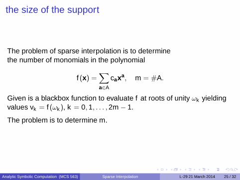
the size of the support

The problem of sparse interpolation is to determinethe number of monomials in the polynomial

f (x) =∑

a∈A

caxa, m = #A.

Given is a blackbox function to evaluate f at roots of unity ωk yieldingvalues vk = f (ωk ), k = 0, 1, . . . , 2m − 1.

The problem is to determine m.


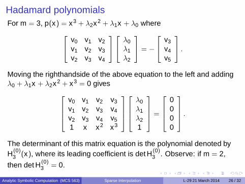
Hadamard polynomialsFor m = 3, p(x) = x3 + λ2x2 + λ1x + λ0 where

v0 v1 v2

v1 v2 v3

v2 v3 v4

λ0

λ1

λ2

= −

v3

v4

v5

.

Moving the righthandside of the above equation to the left and addingλ0 + λ1x + λ2x2 + x3 = 0 gives

v0 v1 v2 v3

v1 v2 v3 v4

v2 v3 v4 v5

1 x x2 x3

λ0

λ1

λ2

1

=

0000

.

The determinant of this matrix equation is the polynomial denoted byH(0)

3 (x), where its leading coefficient is det H(0)3 . Observe: if m = 2,

then det H(0)3 = 0.


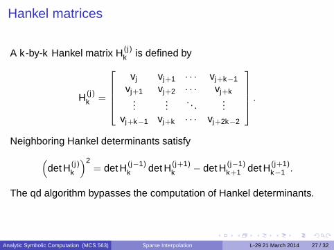
Hankel matrices

A k-by-k Hankel matrix H(j)k is defined by

H(j)k =

vj vj+1 · · · vj+k−1

vj+1 vj+2 · · · vj+k...

.... . .

...vj+k−1 vj+k · · · vj+2k−2

.

Neighboring Hankel determinants satisfy

(det H(j)

k

)2= det H(j−1)

k det H(j+1)k − det H(j−1)

k+1 det H(j+1)k−1 .

The qd algorithm bypasses the computation of Hankel determinants.


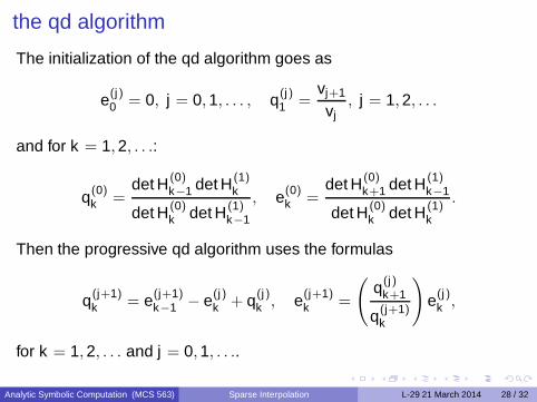
the qd algorithm

The initialization of the qd algorithm goes as

e(j)0 = 0, j = 0, 1, . . . , q(j)

1 =vj+1

vj, j = 1, 2, . . .

and for k = 1, 2, . . .:

q(0)k =

det H(0)k−1 det H(1)

k

det H(0)k det H(1)

k−1

, e(0)k =

det H(0)k+1 det H(1)

k−1

det H(0)k det H(1)

k

.

Then the progressive qd algorithm uses the formulas

q(j+1)k = e(j+1)

k−1 − e(j)k + q(j)

k , e(j+1)k =

(q(j)

k+1

q(j+1)k

)e(j)

k ,

for k = 1, 2, . . . and j = 0, 1, . . ..


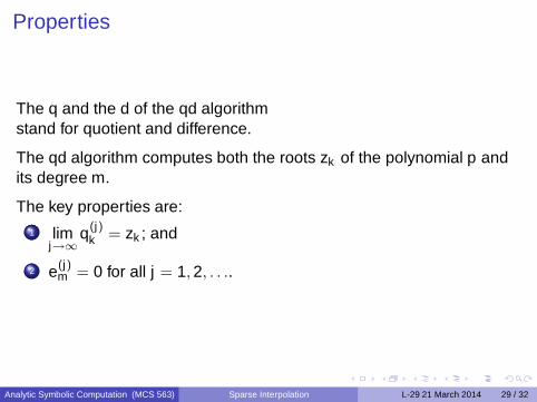
Properties

The q and the d of the qd algorithmstand for quotient and difference.

The qd algorithm computes both the roots zk of the polynomial p andits degree m.

The key properties are:

1 limj→∞

q(j)k = zk ; and

2 e(j)m = 0 for all j = 1, 2, . . ..


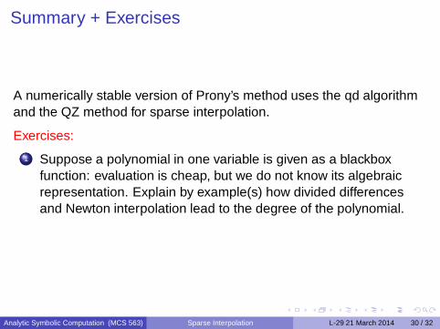
Summary + Exercises

A numerically stable version of Prony’s method uses the qd algorithmand the QZ method for sparse interpolation.

Exercises:

1 Suppose a polynomial in one variable is given as a blackboxfunction: evaluation is cheap, but we do not know its algebraicrepresentation. Explain by example(s) how divided differencesand Newton interpolation lead to the degree of the polynomial.


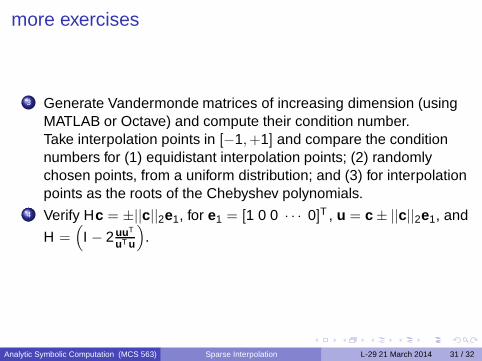
more exercises

3 Generate Vandermonde matrices of increasing dimension (usingMATLAB or Octave) and compute their condition number.Take interpolation points in [−1,+1] and compare the conditionnumbers for (1) equidistant interpolation points; (2) randomlychosen points, from a uniform distribution; and (3) for interpolationpoints as the roots of the Chebyshev polynomials.

4 Verify Hc = ±||c||2e1, for e1 = [1 0 0 · · · 0]T , u = c ± ||c||2e1, and

H =(

I − 2uuT

uT u

).


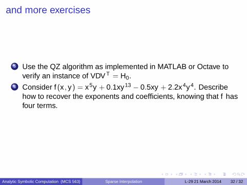
and more exercises

5 Use the QZ algorithm as implemented in MATLAB or Octave toverify an instance of VDV T = H0.

6 Consider f (x , y) = x5y + 0.1xy13 − 0.5xy + 2.2x4y4. Describehow to recover the exponents and coefficients, knowing that f hasfour terms.


Sparse Interpolation - University of Illinois at...

Documents

Transcript of Sparse Interpolation - University of Illinois at...