
Spacetime models in R-INLAelias/cursos/br2015/inla_spacetime.pdf · —kronecker product model...
26
Transcript of Spacetime models in R-INLAelias/cursos/br2015/inla_spacetime.pdf · —kronecker product model...
2
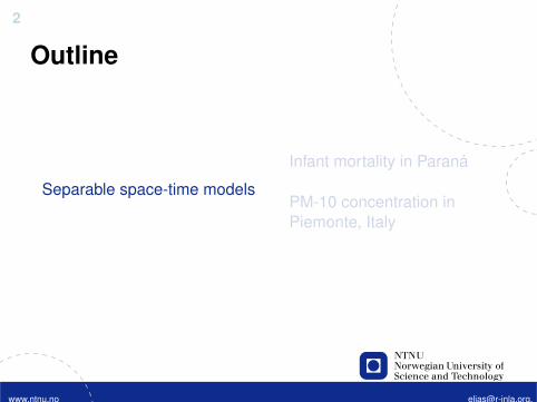
Outline
Separable space-time models
Infant mortality in Paraná
PM-10 concentration inPiemonte, Italy
www.ntnu.no [email protected],
3
Multivariate dynamic regression model— y t : n observations at time t , E(y t ) = µt
µt = g−1(diag(F ′t (x t + µx )))x t = Gtx t−1 + ωt (1)
• diag(·): only diagonal of F ′tx t counts• g(·): link function, g−1(·): inverse link• F t : p × n covariate matrix at each time t• x t : p × n latent (unobservable) states• Gt : p × p matrix to describe time evolution• ωt : p × n dimensional vector of errors• E(x) = 0 and µx are fixed effects
www.ntnu.no [email protected],
4
Remarks
— ωt : p vectors {ωt1, ...,ωtp}, each with length n— each vector in {ωt1, ...,ωtp}, ωtj ∼ MVNormal(0,Σ j )— possible in R-INLA
• y t : several likelihoods• Σk : some spatial models• Gt = G (fixed over time), and diagonal: AR(1) for each state
— implementation in R-INLA• kronecker product model (for some models)• ’facked’ zero observations (for all and 2nd dynamic models)
www.ntnu.no [email protected],
5
Kronecker product models
— x = {x11, ..., xn1, x12, ..., xnT}— assume
π(x) ∝ (|Q1⊗Q2|∗)1/2 exp(−1
2xT{Q1⊗Q2}x
)where |.|∗ is the generalized determinant
— kronecker product model example in R-INLA
f(spatial, model='besagproper2',group=time, control.group=list(model='ar1'))
www.ntnu.no [email protected],
6
Spacetime interactions
— kronecker product models follows Clayton’s rule— combine Q1 and Q2 available— warning care when main effects are in the model— WARNING super care when Q1 and/or Q2 have rank
deficiency— the described dynamic model is type IV and uses Q2 as AR(1)
www.ntnu.no [email protected],

7
Outline
Separable space-time models
Infant mortality in Paraná
PM-10 concentration inPiemonte, Italy
www.ntnu.no [email protected],
8
Infant mortality model— infant death at municipality i and year t
yit ∼ Poisson(Eiteηit )
— Ei : expected number of death (under some suposition)• overal ratio
r0 =∑
it yit∑it bornsit
• Eit = r0bornsit• Eit : expected deaths if the ratio is the same
(over space and time)• observed relative risk
SMRit =yit
Eit
www.ntnu.no [email protected],
9
Model structure— linear predictor evolution over time
xit = ρxi,t−1 + sit
— sit at each time→ spatially correlated
sit |s−i,t ∼ N(∑j∼i
sj,t/ni , σ2s/ni )
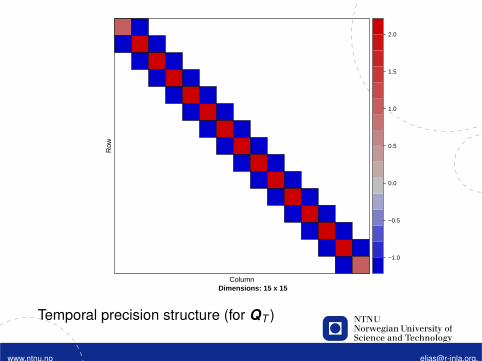
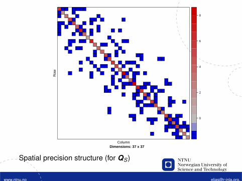
— space-time precision matrix implied: Q = QT ⊗QS— both smooth over time and space (if ρ is near 1)— the full model (type IV)
ηit = α0 + et + ui + vt + si + xit
where• α0 is the intercept• et is a unstructured temporal random effect• ui is a unstructured spatial random effect• vt is a structured temporal random effect• st is a structured temporal random effect• xit is a space-time random effect
www.ntnu.no [email protected],
10
On space-time random effect
— it can be one of the four type interaction models— dynamic model using the besagproper2 model for space
• λ = 0: no spatial structure• λ = 1: equals the intrinsic Besag• ρ = 0: no temporal structure• ρ = 1: equals RW1• → includes all the four interaction types
www.ntnu.no [email protected],
Dimensions: 15 x 15Column
Row
−1.0
−0.5
0.0
0.5
1.0
1.5
2.0
Temporal precision structure (for QT )
www.ntnu.no [email protected],
Dimensions: 37 x 37Column
Row
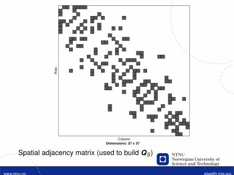
Spatial adjacency matrix (used to build QS)
www.ntnu.no [email protected],
Dimensions: 37 x 37Column
Row
0
2
4
6
8
Spatial precision structure (for QS)
www.ntnu.no [email protected],
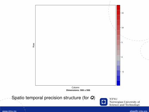
Dimensions: 555 x 555Column
Row
−5
0
5
10
15
Spatio temporal precision structure (for Q)
www.ntnu.no [email protected],
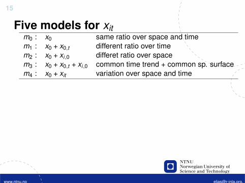
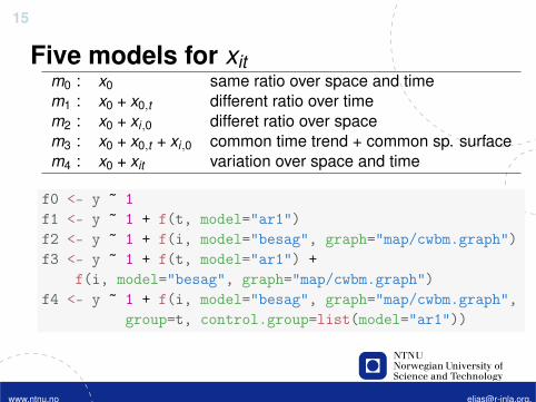
15
Five models for xitm0 : x0 same ratio over space and timem1 : x0 + x0,t different ratio over timem2 : x0 + xi,0 differet ratio over spacem3 : x0 + x0,t + xi,0 common time trend + common sp. surfacem4 : x0 + xit variation over space and time
f0 <- y ~ 1f1 <- y ~ 1 + f(t, model="ar1")f2 <- y ~ 1 + f(i, model="besag", graph="map/cwbm.graph")f3 <- y ~ 1 + f(t, model="ar1") +
f(i, model="besag", graph="map/cwbm.graph")f4 <- y ~ 1 + f(i, model="besag", graph="map/cwbm.graph",
group=t, control.group=list(model="ar1"))
www.ntnu.no [email protected],

16
Outline
Separable space-time models
Infant mortality in Paraná
PM-10 concentration inPiemonte, Italy
www.ntnu.no [email protected],
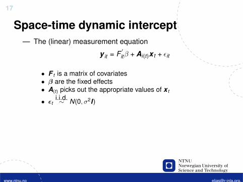
17
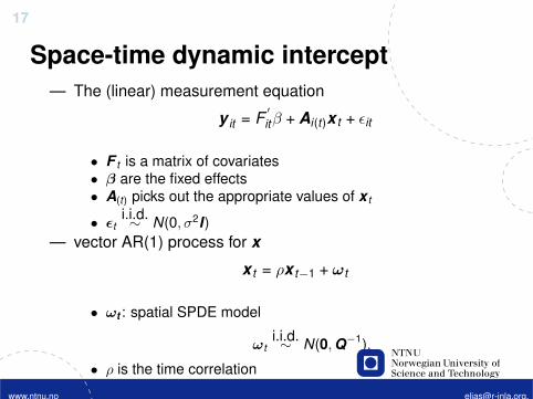
Space-time dynamic intercept— The (linear) measurement equation
y it = F′
itβ + Ai(t)x t + εit
• F t is a matrix of covariates• β are the fixed effects• A(t) picks out the appropriate values of x t
• εti.i.d.∼ N(0, σ2I)
— vector AR(1) process for x
x t = ρx t−1 + ωt
• ωt : spatial SPDE model
ωti.i.d.∼ N(0,Q−1),
• ρ is the time correlation
www.ntnu.no [email protected],
17
Space-time dynamic intercept— The (linear) measurement equation
y it = F′
itβ + Ai(t)x t + εit
• F t is a matrix of covariates• β are the fixed effects• A(t) picks out the appropriate values of x t
• εti.i.d.∼ N(0, σ2I)
— vector AR(1) process for x
x t = ρx t−1 + ωt
• ωt : spatial SPDE model
ωti.i.d.∼ N(0,Q−1),
• ρ is the time correlation
www.ntnu.no [email protected],

18
PM-10 concentration in Piemonte, Italy
Cameletti et al. (2011), on r-inla.org
— 24 monitoring stations— Daily data from 10/05 to 03/06
www.ntnu.no [email protected],
19
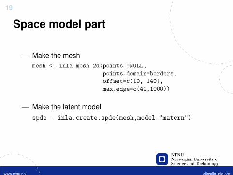
Space model part
— Make the meshmesh <- inla.mesh.2d(points =NULL,
points.domain=borders,offset=c(10, 140),max.edge=c(40,1000))
— Make the latent modelspde = inla.create.spde(mesh,model="matern")
www.ntnu.no [email protected],
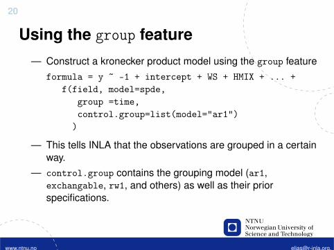
20
Using the group feature— Construct a kronecker product model using the group feature
formula = y ~ -1 + intercept + WS + HMIX + ... +f(field, model=spde,
group =time,control.group=list(model="ar1")
)
— This tells INLA that the observations are grouped in a certainway.
— control.group contains the grouping model (ar1,exchangable, rw1, and others) as well as their priorspecifications.
www.ntnu.no [email protected],

21
Make an A matrix
— Use the group argumentLocationMatrix = inla.spde.make.A(mesh = mesh,
loc =dataLoc, group=time, n.group=nT)
— data locations in all group=time level— builds an A matrix in an appropriate way
www.ntnu.no [email protected],

22
Organising the dataCovariates at the data points, but the latent field only defined theirthrough the A matrixWe need to make sure that A only applies to the random effect.
idx.set <- inla.spde.make.index("mesh.idx",n.field=nmesh,n.group=T)
stack = inla.stack( data = dat,A = list(1, LocationMatrix),effects = list( list(WS = cov$WS,...),
c(idx.set,list(intercept=rep(1,mesh$n*nT)))
))
www.ntnu.no [email protected],