Space ChargeLuigi Palumbo

Università di Roma "La Sapienza"and LNF-INFN

CAS, 25 May 2005CAS, 25 May 2005

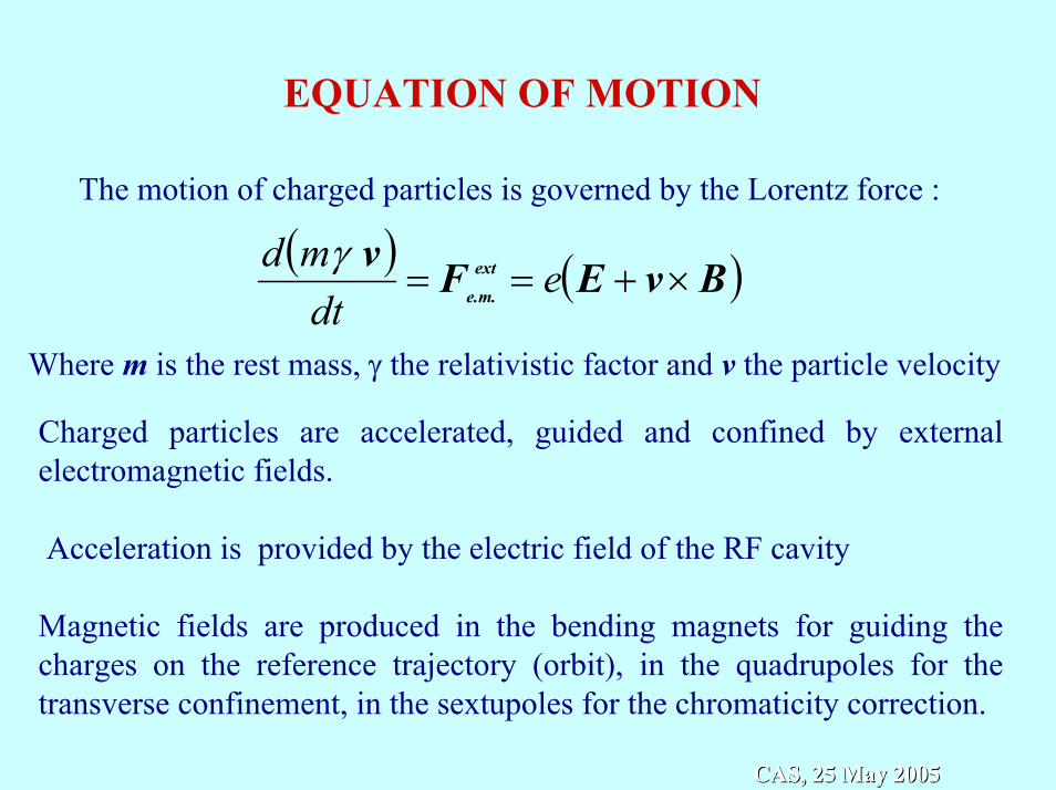
EQUATION OF MOTION

The motion of charged particles is governed by the Lorentz force :

( ) ( )BvEFv ext

e.m. ×+== edt

md γ

Where m is the rest mass, γ the relativistic factor and v the particle velocity

Charged particles are accelerated, guided and confined by external electromagnetic fields.

Acceleration is provided by the electric field of the RF cavity

Magnetic fields are produced in the bending magnets for guiding the charges on the reference trajectory (orbit), in the quadrupoles for the transverse confinement, in the sextupoles for the chromaticity correction.

CAS, 25 May 2005CAS, 25 May 2005

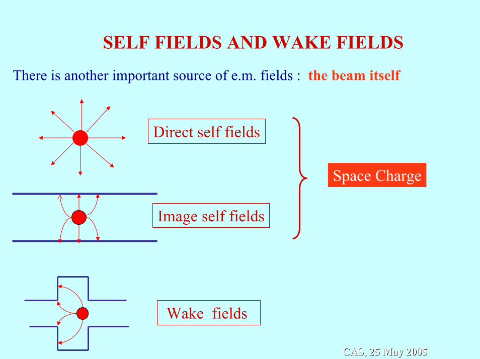
SELF FIELDS AND WAKE FIELDS

There is another important source of e.m. fields : the beam itself

Direct self fields

Space Charge

Image self fields

Wake fields

CAS, 25 May 2005CAS, 25 May 2005

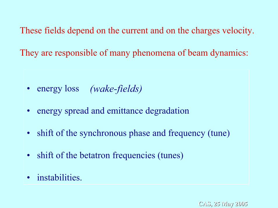
These fields depend on the current and on the charges velocity.

They are responsible of many phenomena of beam dynamics:

• energy loss

• energy spread and emittance degradation

• shift of the synchronous phase and frequency (tune)

• shift of the betatron frequencies (tunes)

• instabilities.

(wake-fields)

CAS, 25 May 2005CAS, 25 May 2005

Fields of a point charge with uniform motion

o

z

x,x’

y

o’

z’

y’

v

q

0

4 3

=′′

′=′

BrrqE

or

rr

πε

vt is the position of the point charge in the lab. frame O.

• In the moving frame O’ the charge is at rest• The electric field is radial with spherical symmetry• The magnetic field is zero

34 rzqE

oz

′

′=′

πε34 ryqE

oy

′

′=′

πε34 rxqE

ox

′

′=′

πε

CAS, 25 May 2005CAS, 25 May 2005

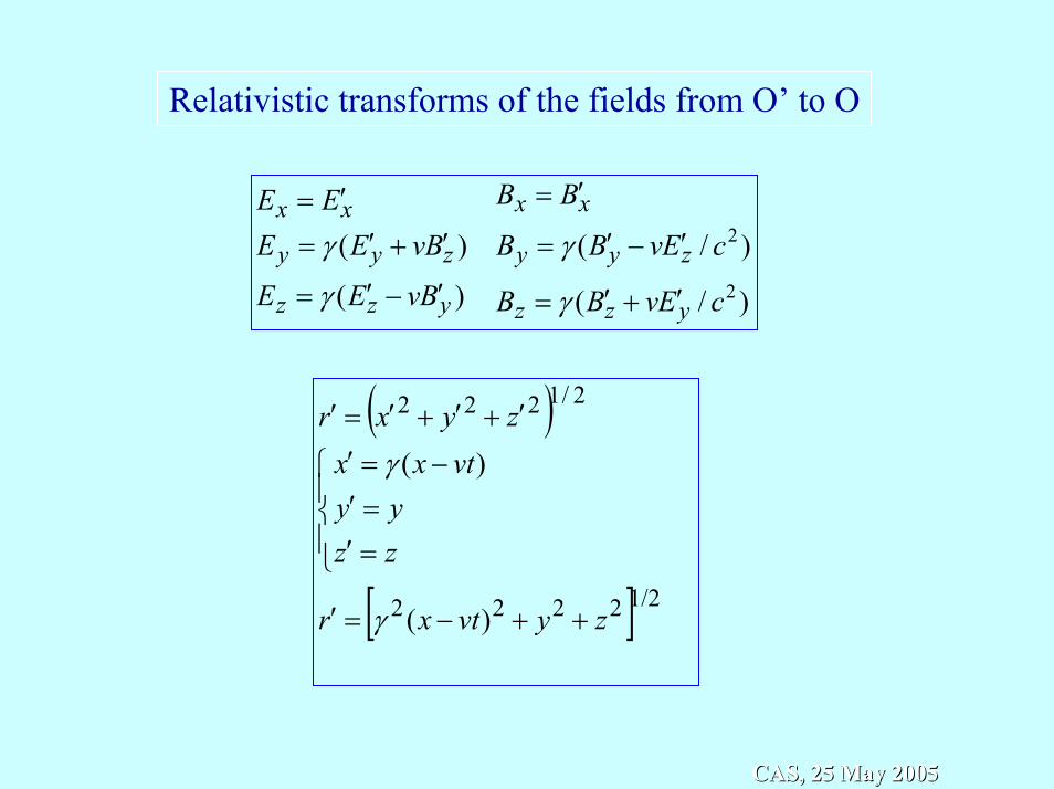
Relativistic transforms of the fields from O’ to O

)/(

)/(

)(

)(2

2

cEvBB

cEvBB

BB

BvEE

BvEEEE

yzz

zyy

xx

yzz

zyy

xx

′+′=

′−′=

′=

′−′=

′+′=

′=

γ

γ

γ

γ

( )

[ ] )(

)(

1/22222

2/1222

zyvtxr

zzyy

vtxxzyxr

++−=′

=′=′

−=′

′+′+′=′

γ

γ

CAS, 25 May 2005CAS, 25 May 2005

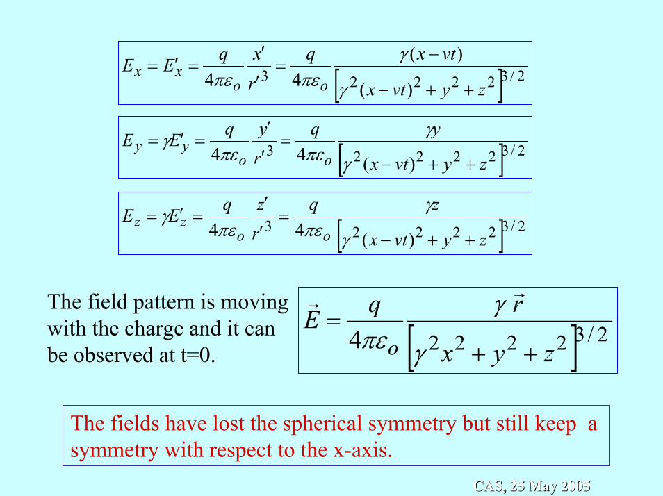
[ ] 2/322223)(

)(44 zyvtx

vtxqrxqEE

ooxx

++−

−=

′

′=′=

γ

γπεπε

[ ] 2/322223)(44 zyvtx

yqryqEE

ooyy

++−=

′

′=′=

γ

γπεπε

γ

[ ] 2/322223)(44 zyvtx

zqrzqEE

oozz

++−=

′

′=′=

γ

γπεπε

γ

[ ] 2/32222

4 zyx

rqEo ++

=γ

γπε

rrThe field pattern is moving with the charge and it can be observed at t=0.

The fields have lost the spherical symmetry but still keep a symmetry with respect to the x-axis.

CAS, 25 May 2005CAS, 25 May 2005

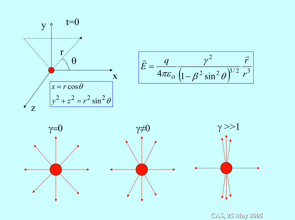
t=0

x

y

z

rθ

θ

θ2222 sin

cos

rzy

rx

=+

=( ) 32/322

2

sin1

4 r

rqEo

rr

θβ

γπε −

=

γ >>1γ≠0γ=0

CAS, 25 May 2005CAS, 25 May 2005

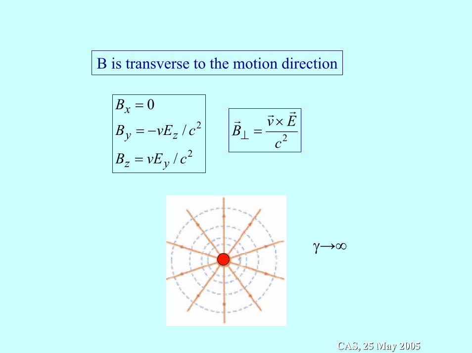
B is transverse to the motion direction

2

2

/

/

0

cvEB

cvEB

B

yz

zy

x

=

−=

=

2cEvBrrr ×

=⊥

γ→∞

CAS, 25 May 2005CAS, 25 May 2005

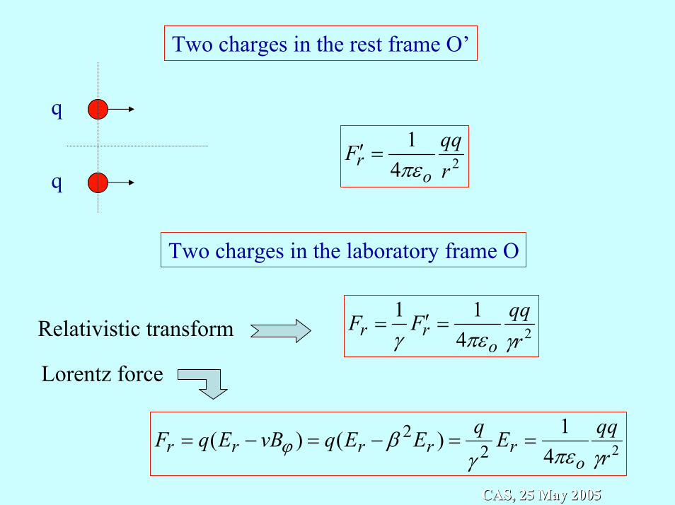
Two charges in the rest frame O’

q

q

241

rqqF

or πε

=′

2411

rqqFF

orr γπεγ

=′=

Two charges in the laboratory frame O

Relativistic transform

Lorentz force

241)()( 2

2rqqEqEEqvBEqF

orrrrr γπεγ

βϕ ==−=−=

CAS, 25 May 2005CAS, 25 May 2005

Direct Space Charge Forces

CAS, 25 May 2005CAS, 25 May 2005

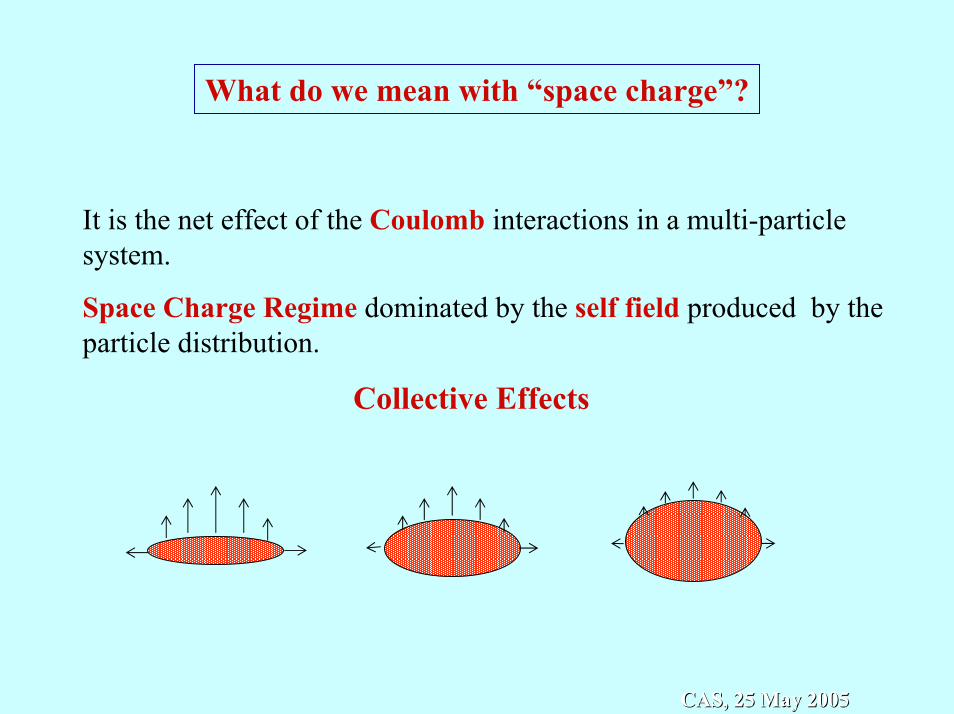
It is the net effect of the Coulomb interactions in a multi-particle system.

Space Charge Regime dominated by the self field produced by the particle distribution.

Collective Effects

CAS, 25 May 2005CAS, 25 May 2005

What do we mean with “space charge”?

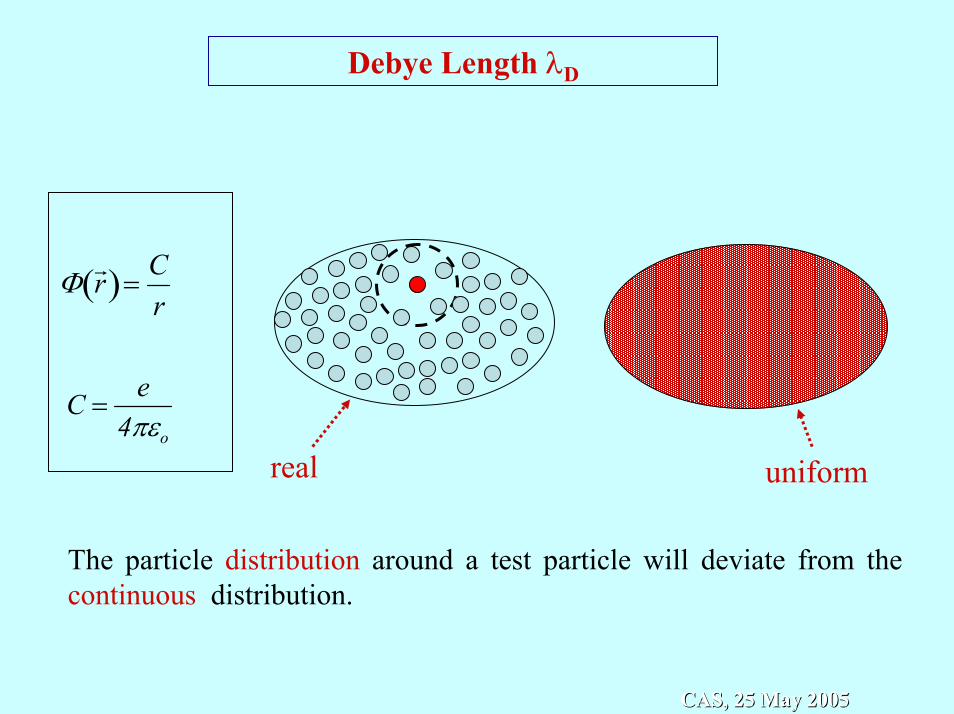
Debye Length λD

Φ

r r ( )=

Cr

C =e

4πεo

real uniform

The particle distribution around a test particle will deviate from the continuous distribution.

CAS, 25 May 2005CAS, 25 May 2005

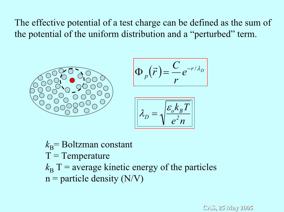
The effective potential of a test charge can be defined as the sum of the potential of the uniform distribution and a “perturbed” term.

( ) Drp e

rCr λ/−=Φ

r

λD =εokBTe2n

kB= Boltzman constantT = TemperaturekB T = average kinetic energy of the particlesn = particle density (N/V)

CAS, 25 May 2005CAS, 25 May 2005

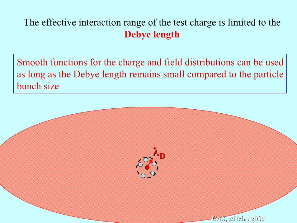
The effective interaction range of the test charge is limited to the Debye length

λλDD

CAS, 25 May 2005CAS, 25 May 2005

Smooth functions for the charge and field distributions can be used as long as the Debye length remains small compared to the particle bunch size

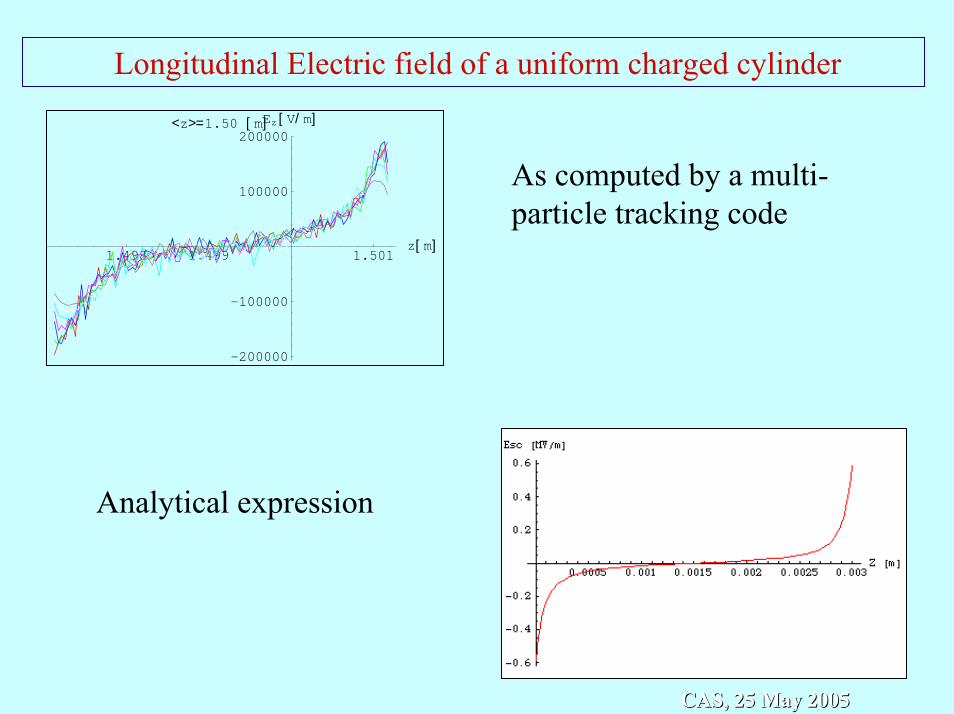
Longitudinal Electric field of a uniform charged cylinder

1.498 1.499 1.501z[ m]

-200000

-100000

100000

200000Ez [ V/ m]<z>=1.50 [ m]

As computed by a multi-particle tracking code

Analytical expression

CAS, 25 May 2005CAS, 25 May 2005

Space charge of a relativistic cylindrical distribution

L

RCylindrical finite bunch, uniformly charged,With circular cross section

-0.002 0.002 0.004 0.006

1

2

3

4

5Er

-0.002 0.002 0.004 0.006

-1.5

-1

-0.5

0.5

1

1.5EzTransverse electric field at r = a

Longitudinal electric field at r = 0

CAS, 25 May 2005CAS, 25 May 2005

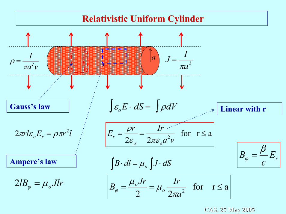
Relativistic Uniform Cylinder

εoE ⋅ dS = ρdV∫∫

arfor 22 2 ≤==

vaIrrEoo

r πεερlrErl ro

22 ρπεπ =

J =I

πa2ρ =I

πa2va

Gauss’s law Linear with r

rEc

B βϕ =

Ampere’s law ∫ ∫ ⋅=⋅ dSJdlB oµ

arfor 22 2 ≤==

aIrJrB o

o

πµµ

ϕJlrlB oµϕ =2

CAS, 25 May 2005CAS, 25 May 2005

)/(2 mCao ρπλ =

2

2

2

)()(B

2

)(

ar

crE

cr

arrE

arfor

o

or

o

or

=

=

=

<

πεβλβ

πελ

θ

2)/()( arr oλλ =

)()/(0

2

2

AcaJImAcJ

λβπ

ρβ

==

=

The Lorentz Force

( ) ( ) 2222

21

areeEEecBEeF

o

orrrr γπε

λγ

ββ ϑ

==−=−=

• has only radial component

• is a linear function of the transverse coordinate

The attractive magnetic force, which becomes significant at highenergy, tends to compensate the repulsive electric force.

CAS, 25 May 2005CAS, 25 May 2005

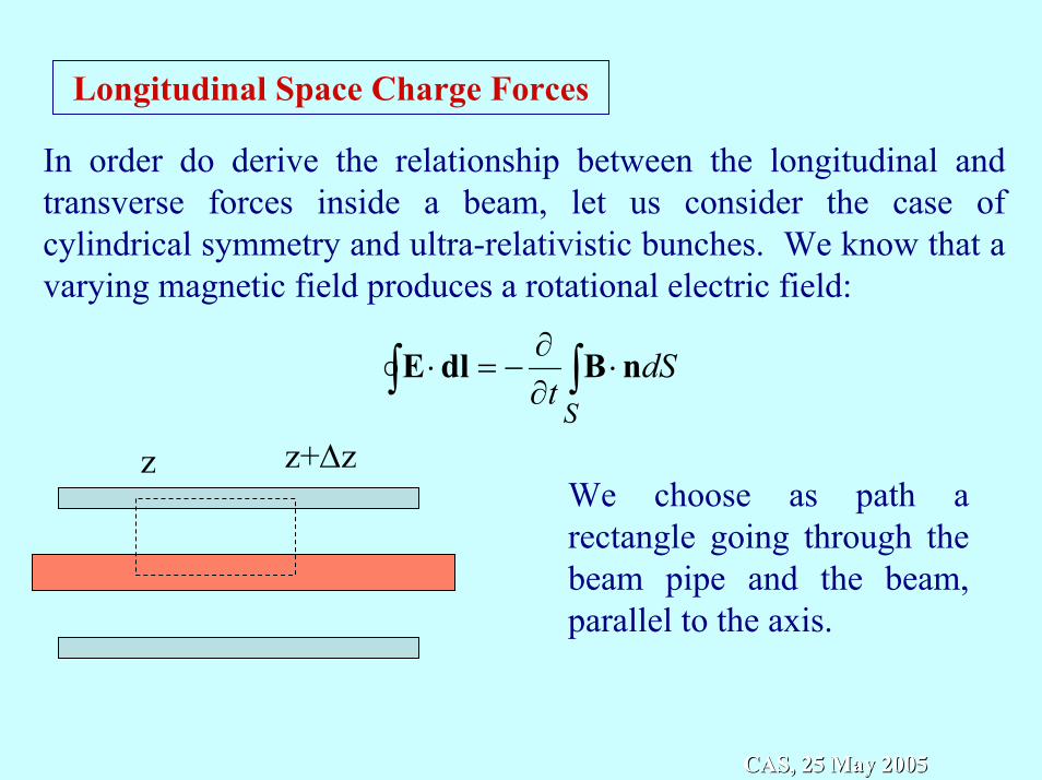
Longitudinal Space Charge Forces

In order do derive the relationship between the longitudinal andtransverse forces inside a beam, let us consider the case of cylindrical symmetry and ultra-relativistic bunches. We know that a varying magnetic field produces a rotational electric field:

∫∫ ⋅∂∂

−=⋅S

dSt

nBdlE

z+∆zzWe choose as path a rectangle going through the beam pipe and the beam, parallel to the axis.

CAS, 25 May 2005CAS, 25 May 2005

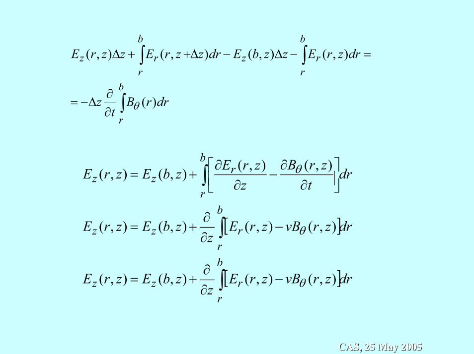
drrBt

z

drzrEzzbEdrzzrEzzrE

b

r

b

rrz

b

rrz

)(

),(),(),(),(

∫

∫∫

∂∂

∆−=

=−∆−∆++∆

θ

[ ]

[ ]drzrvBzrEz

zbEzrE

drzrvBzrEz

zbEzrE

drt

zrBz

zrEzbEzrE

b

rrzz

b

rrzz

b

r

rzz

∫

∫

∫

−∂∂

+=

−∂∂

+=

∂∂

−∂

∂+=

),(),(),(),(

),(),(),(),(

),(),(),(),(

θ

θ

θ

CAS, 25 May 2005CAS, 25 May 2005

∫∂∂

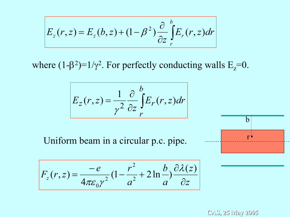
−+=b

rrzz drzrE

zzbEzrE ),()1(),(),( 2β

where (1-β2)=1/γ2. For perfectly conducting walls Ez=0.

∫∂∂

=b

rrz z

12γ

drzrEzrE ),(),(

b

rUniform beam in a circular p.c. pipe.

zz

ab

arezrFz ∂

∂+−

−=

)()ln21(4

),( 2

2

20

λγπε

CAS, 25 May 2005CAS, 25 May 2005

Beam motion in a linear channel

CAS, 25 May 2005CAS, 25 May 2005

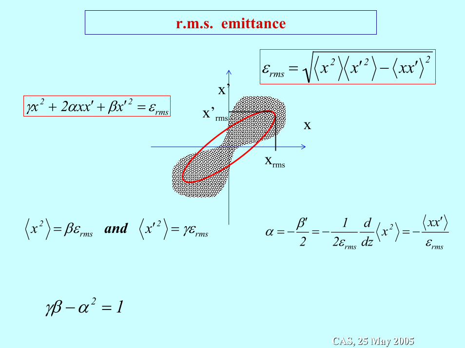
r.m.s. emittance

γx 2 + 2αx ′ x + β ′ x 2 = εrms

x2 = βεrms and ′ x 2 = γεrms α = −′ β

2= −

12εrms

ddz

x2 = −x ′ x εrms

εrms = x2 ′ x 2 − x ′ x 2

x

x’

xrms

x’rms

γβ −α 2 = 1

CAS, 25 May 2005CAS, 25 May 2005

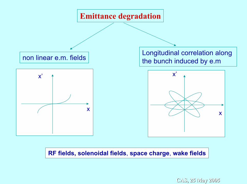
Emittance degradation

Longitudinal correlation along the bunch induced by e.mnon linear e.m. fields

x

x’

x

x’

RF fields, solenoidal fields, space charge, wake fields

CAS, 25 May 2005CAS, 25 May 2005

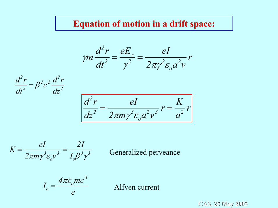
Equation of motion in a drift space:

γm d2rdt2 =

eEr

γ 2 =eI

2πγ 2εoa2v

r

d2rdt2 = β 2c2 d2r

dz2

d2rdz2 =

eI2πmγ 3εoa

2v3 r =Ka2 r

K =eI

2πmγ 3εov3 =

2IIoβ

3γ 3 Generalized perveance

Io =4πεomc3

e Alfven current

CAS, 25 May 2005CAS, 25 May 2005

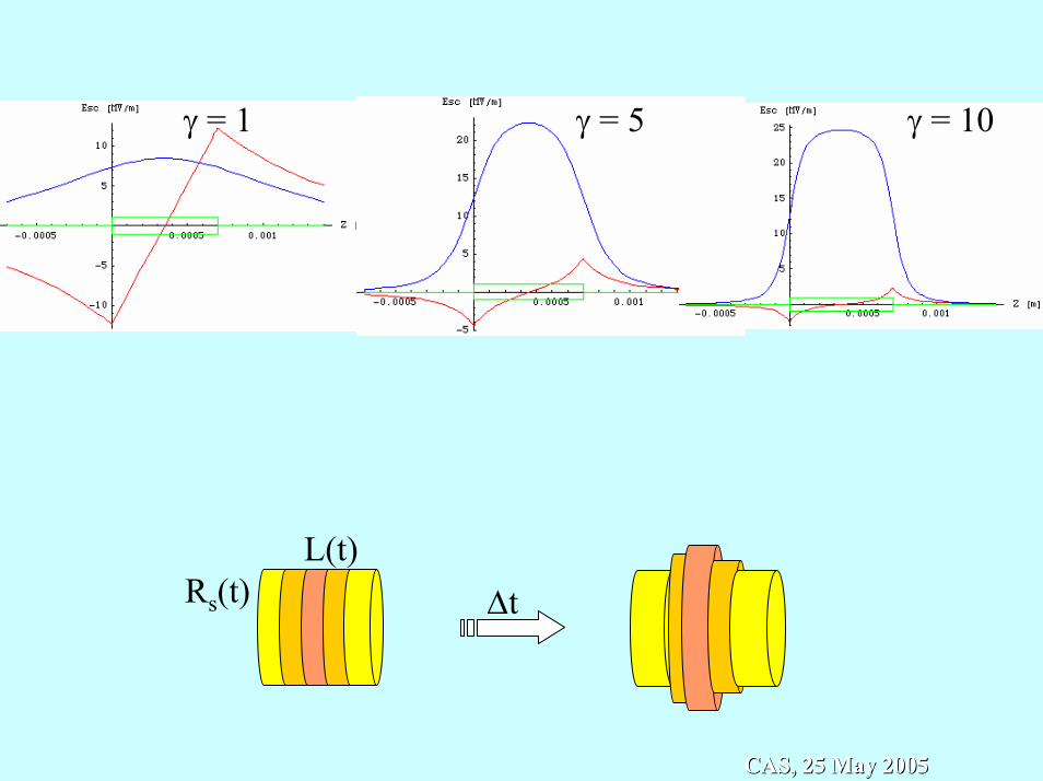
γ = 1 γ = 5 γ = 10

L(t)Rs(t) ∆t

CAS, 25 May 2005CAS, 25 May 2005

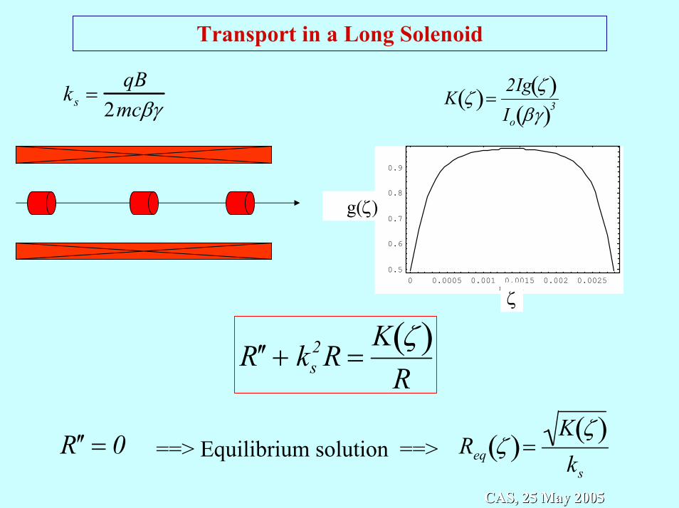
Transport in a Long Solenoid

ks =qB

2mcβγ K ζ( )=2Ig ζ( )Io βγ( )3

0 0.0005 0.001 0.0015 0.002 0.0025metri

0.5

0.6

0.7

0.8

0.9

gg(ζ)

ζ

′ ′ R + ks2R =

K ζ( )R

==> Equilibrium solution ==>′ ′ R = 0 Req ζ( )=K ζ( )ks

CAS, 25 May 2005CAS, 25 May 2005

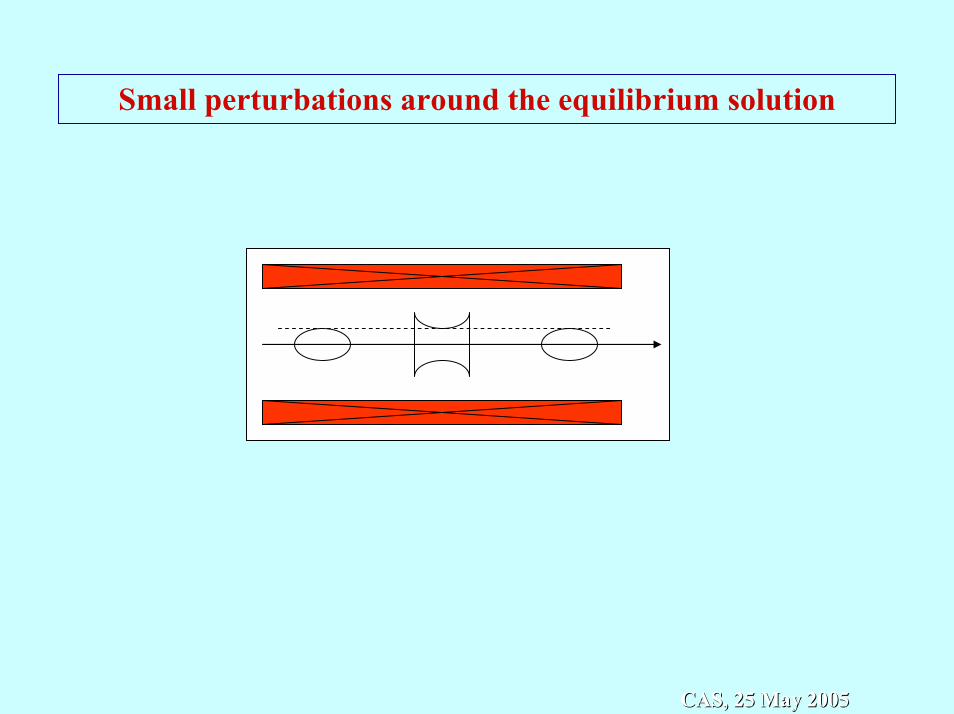
Small perturbations around the equilibrium solution

CAS, 25 May 2005CAS, 25 May 2005

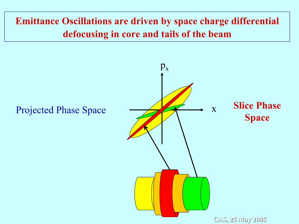
Emittance Oscillations are driven by space charge differential defocusing in core and tails of the beam

x

px

Slice Phase Space

Projected Phase Space

CAS, 25 May 2005CAS, 25 May 2005

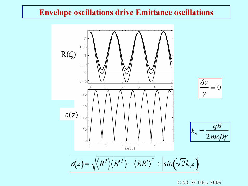
Envelope oscillations drive Emittance oscillations

0 1 2 3 4 5metri

-0.5

0

0.5

1

1.5

2

envelopes

0 1 2 3 4 5metri

0

20

40

60

80

emi

R(ζ)

ε(z)

δγγ

= 0

ks =qB

2mcβγ

ε z( )= R2 ′ R 2 − R ′ R 2 ÷ sin 2ksz( )CAS, 25 May 2005CAS, 25 May 2005

BEAM DYNAMICS MODELING

RF Field + Solenoids

∆t

Space chargeOn Axis

Off Axis∆t

CAS, 25 May 2005CAS, 25 May 2005

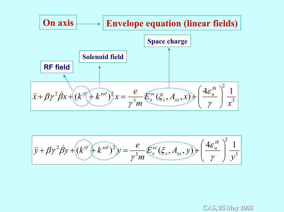
Envelope equation (linear fields)On axis

Space charge

3

2

322 14),,()(

xxAE

mexkkxx

thn

xssscx

solrf

+=+++

γεξ

γββγ &&&

3

2

322 14),,()(

yyAE

meykkyy

thn

xssscx

solrf

+=+++

γεξ

γββγ &&&

RF fieldSolenoid field

CAS, 25 May 2005CAS, 25 May 2005

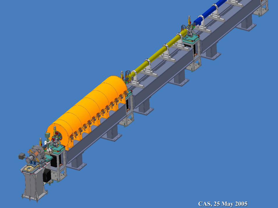
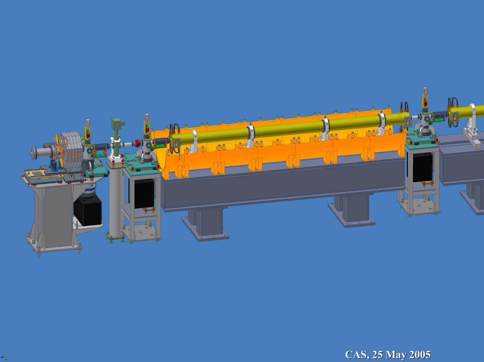
CODES used for simulations of Space Charge Effects

PARMELA, ASTRA

Multi-particle tracking code, includes space charge but not wake fields

HOMDYN

Relies on a multi-envelope model based on the time dependent evolution of a uniform bunch

CAS, 25 May 2005CAS, 25 May 2005

CAS, 25 May 2005CAS, 25 May 2005

CAS, 25 May 2005CAS, 25 May 2005

CAS, 25 May 2005CAS, 25 May 2005

CAS, 25 May 2005CAS, 25 May 2005

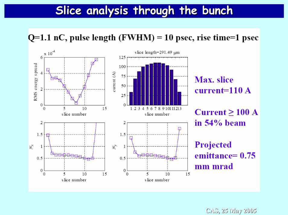
Slice analysis through the bunchSlice analysis through the bunch

CAS, 25 May 2005CAS, 25 May 2005

Space charge with image currents

CAS, 25 May 2005CAS, 25 May 2005

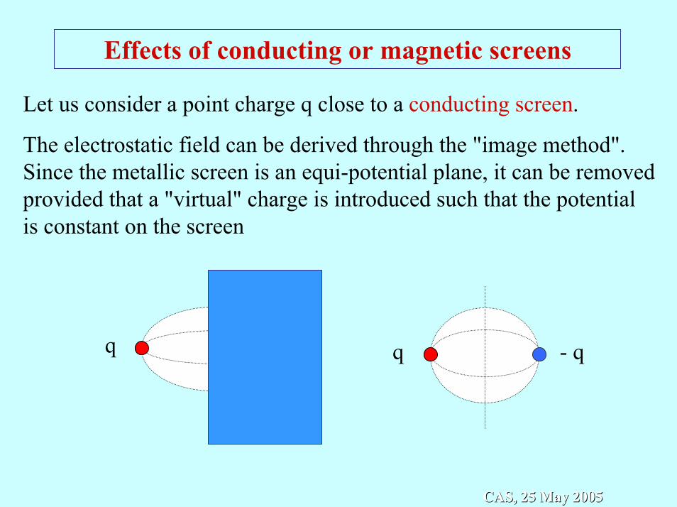
Effects of conducting or magnetic screens

Let us consider a point charge q close to a conducting screen.

The electrostatic field can be derived through the "image method". Since the metallic screen is an equi-potential plane, it can be removed provided that a "virtual" charge is introduced such that the potential is constant on the screen

q q - q

CAS, 25 May 2005CAS, 25 May 2005

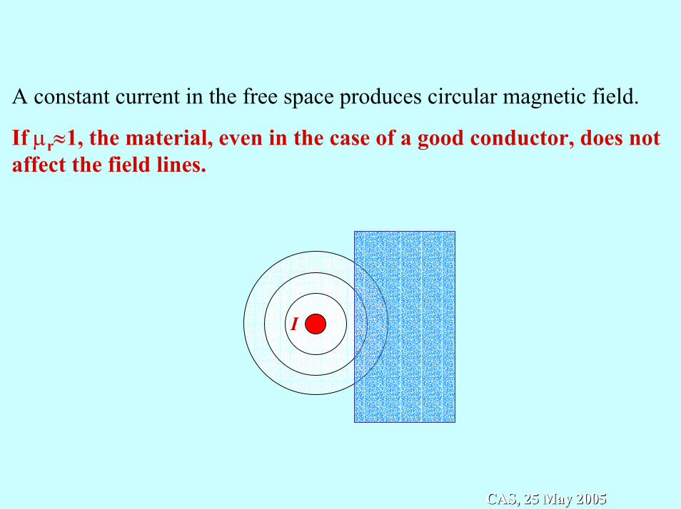
A constant current in the free space produces circular magnetic field.

If µr≈1, the material, even in the case of a good conductor, does not affect the field lines.

I

CAS, 25 May 2005CAS, 25 May 2005

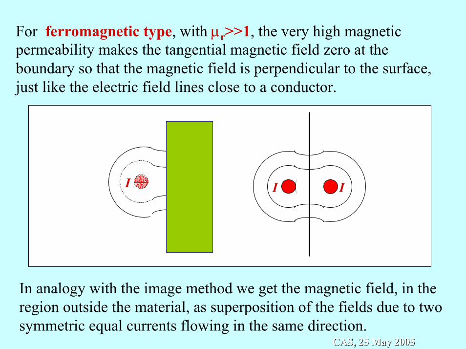
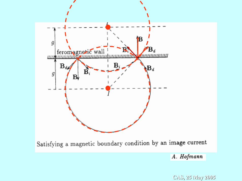
For ferromagnetic type, with µr>>1, the very high magnetic permeability makes the tangential magnetic field zero at the boundary so that the magnetic field is perpendicular to the surface, just like the electric field lines close to a conductor.

I I I

In analogy with the image method we get the magnetic field, in the region outside the material, as superposition of the fields due to two symmetric equal currents flowing in the same direction.

CAS, 25 May 2005CAS, 25 May 2005

CAS, 25 May 2005CAS, 25 May 2005

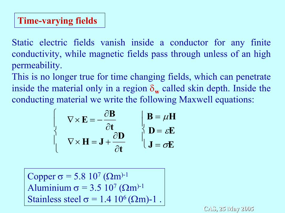
Time-varying fields

Static electric fields vanish inside a conductor for any finite conductivity, while magnetic fields pass through unless of an high permeability. This is no longer true for time changing fields, which can penetrate inside the material only in a region δw called skin depth. Inside the conducting material we write the following Maxwell equations:

∂∂

+=×∇

∂∂

−=×∇

tDJH

tBE

B = µHD = εEJ = σE

Copper σ = 5.8 107 (Ωm)-1

Aluminium σ = 3.5 107 (Ωm)-1

Stainless steel σ = 1.4 106 (Ωm)-1 .CAS, 25 May 2005CAS, 25 May 2005

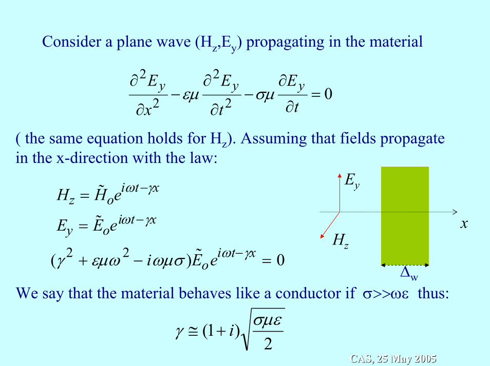
Consider a plane wave (Hz,Ey) propagating in the material

02

2

2

2=

∂

∂−

∂

∂−

∂

∂

tE

t

E

x

E yyy σµεµ

( the same equation holds for Hz). Assuming that fields propagate in the x-direction with the law:

Hz = ˜ H oeiωt−γx

Ey = ˜ E oeiωt−γx

(γ 2 + εµω 2 − iωµσ ) ˜ E oeiωt−γx = 0

We say that the material behaves like a conductor if σ>>ωε thus:∆w

Ey

xHz

2)1( σµεγ i+≅

CAS, 25 May 2005CAS, 25 May 2005

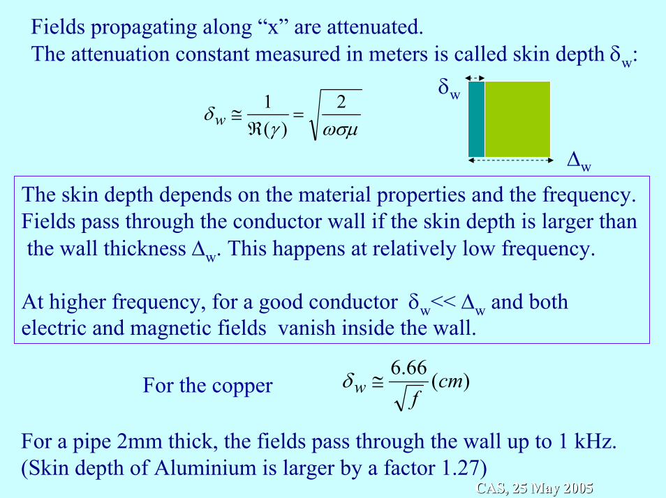
Fields propagating along “x” are attenuated. The attenuation constant measured in meters is called skin depth δw:

δw

ωσµγδ 2

)(1

=ℜ

≅w

∆w

The skin depth depends on the material properties and the frequency.Fields pass through the conductor wall if the skin depth is larger than the wall thickness ∆w. This happens at relatively low frequency.

At higher frequency, for a good conductor δw<< ∆w and both electric and magnetic fields vanish inside the wall.

)(66.6 cmfw ≅δFor the copper

For a pipe 2mm thick, the fields pass through the wall up to 1 kHz. (Skin depth of Aluminium is larger by a factor 1.27)

CAS, 25 May 2005CAS, 25 May 2005

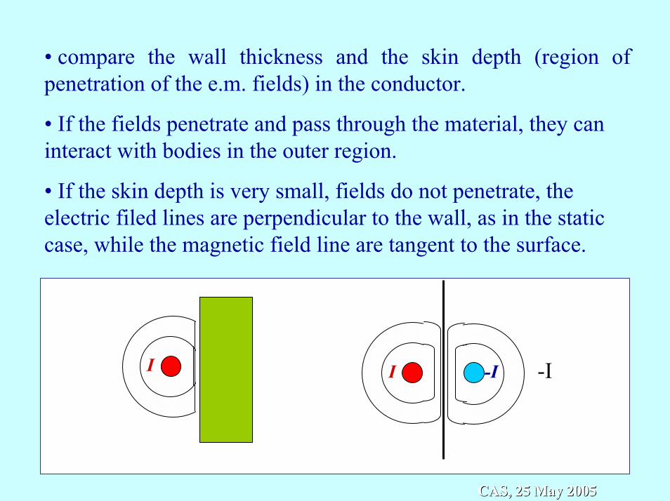
• compare the wall thickness and the skin depth (region of penetration of the e.m. fields) in the conductor.

• If the fields penetrate and pass through the material, they caninteract with bodies in the outer region.

• If the skin depth is very small, fields do not penetrate, the electric filed lines are perpendicular to the wall, as in the static case, while the magnetic field line are tangent to the surface.

I -II -I

CAS, 25 May 2005CAS, 25 May 2005

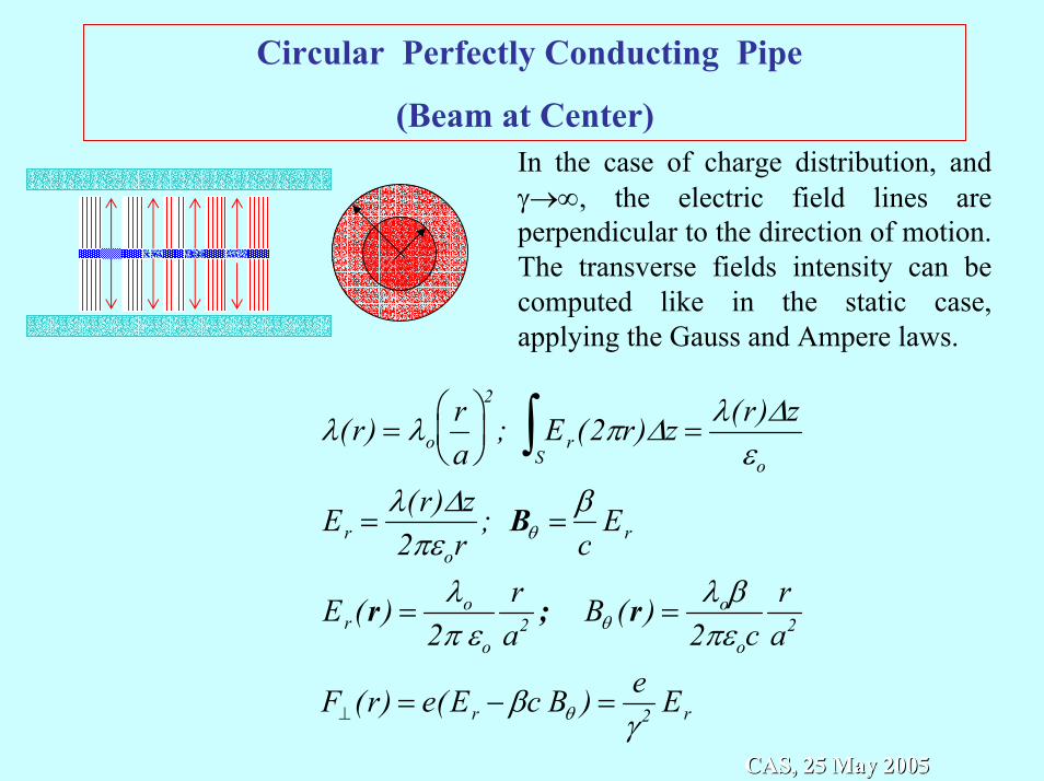
Circular Perfectly Conducting Pipe

(Beam at Center)In the case of charge distribution, and γ→∞, the electric field lines are perpendicular to the direction of motion. The transverse fields intensity can be computed like in the static case, applying the Gauss and Ampere laws.

λ(r) = λora

2

; ErS

∫ (2πr)∆z =λ(r)∆z

εo

Er =λ(r)∆z2πεor

; Bθ =βc

Er

Er(r) =λo

2π εo

ra2 ; Bθ (r ) =

λoβ2πεoc

ra2

F⊥ (r) = e(Er − βc Bθ ) =eγ 2 Er

CAS, 25 May 2005CAS, 25 May 2005

• Due to the symmetry, the transverse fields produced by an ultra-relativistic charge inside the pipe are the same as in the free space.

• For a distribution with cylindrical symmetry, in the ultra-relativistic regime, there is a cancellation of the electric andmagnetic forces.

• The uniform beam produces exactly the same forces as in the free space.

• This result does not depend on the longitudinal distribution of the beam. In general one has to consider the local charge density λ(z)

CAS, 25 May 2005CAS, 25 May 2005

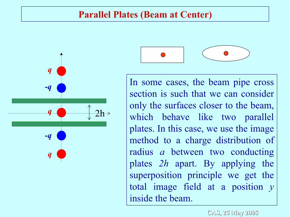
Parallel Plates (Beam at Center)

2hq

q

q

-q

-q In some cases, the beam pipe cross section is such that we can consider only the surfaces closer to the beam, which behave like two parallel plates. In this case, we use the image method to a charge distribution of radius a between two conducting plates 2h apart. By applying the superposition principle we get the total image field at a position yinside the beam.

CAS, 25 May 2005CAS, 25 May 2005

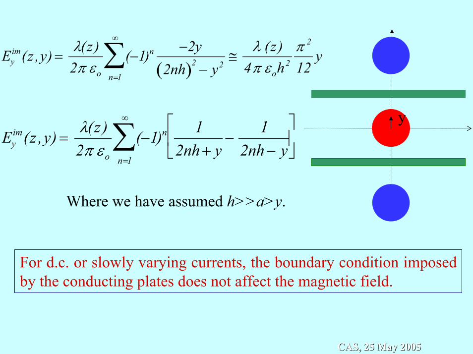
Eyim(z ,y) =

λ(z )2π εo

(−1)n

n=1

∞

∑ −2y2nh( )2 − y2

≅λ (z)

4π εoh2

π 2

12y

yEy

im(z ,y) =λ(z )2π εo

(−1)n

n=1

∞

∑ 12nh + y

−1

2nh − y

Where we have assumed h>>a>y.

For d.c. or slowly varying currents, the boundary condition imposed by the conducting plates does not affect the magnetic field.

CAS, 25 May 2005CAS, 25 May 2005

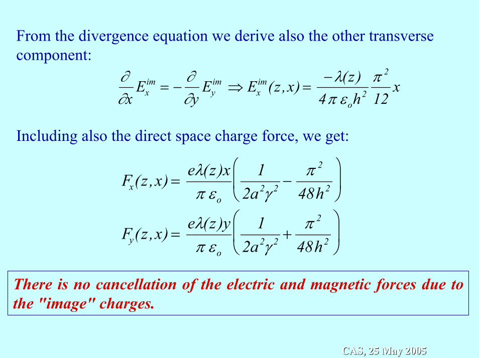
From the divergence equation we derive also the other transversecomponent:

∂∂x

Exim = −

∂∂y

Eyim ⇒ Ex

im(z ,x) =−λ(z )

4π εoh2

π 2

12x

Including also the direct space charge force, we get:

Fx(z ,x) =eλ(z )xπ εo

12a2γ 2 −

π 2

48h2

Fy(z ,x) =eλ(z )yπ εo

12a2γ 2 +

π 2

48h2

There is no cancellation of the electric and magnetic forces due to the "image" charges.

CAS, 25 May 2005CAS, 25 May 2005

Parallel Plates (Beam at Center) a.c. currents

Usually, the frequency beam spectrum is quite rich of harmonics,especially for bunched beams.

It is convenient to decompose the current into a d.c. component, I, for which δw>>∆w, and an a.c. component, Î, for which δw<< ∆w.

While the d.c. component of the magnetic does not perceives the presence of the material, its a.c. component is obliged to be tangent at the wall. For a charge density λ we have I=λv.

We can see that this current produces a magnetic field able to cancel the effect of the electrostatic force.

CAS, 25 May 2005CAS, 25 May 2005

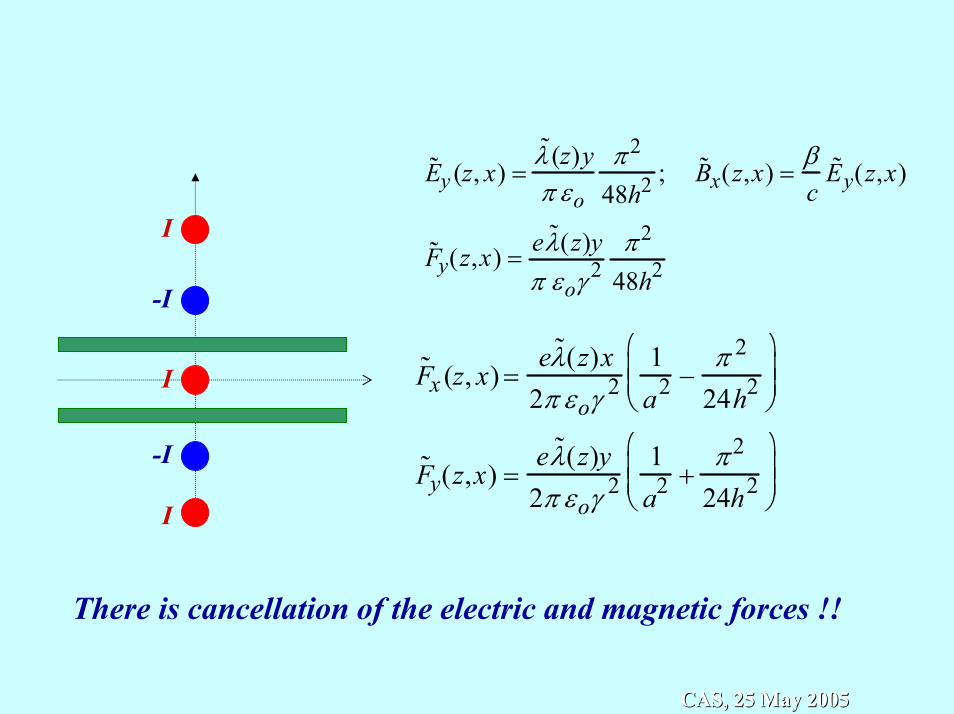
˜ E y (z, x) =˜ λ (z)yπ εo

π 2

48h2 ; ˜ B x(z,x) =βc

˜ E y(z,x)

˜ F y(z,x) = e ˜ λ (z)yπ εoγ 2

π 2

48h2

I

-I

-I

I

I

˜ F x (z, x) =e ˜ λ (z)x

2π εoγ 21a2 −

π 2

24h2

˜ F y(z,x) =e ˜ λ (z)y2π εoγ 2

1a2 +

π 2

24h2

There is cancellation of the electric and magnetic forces !!

CAS, 25 May 2005CAS, 25 May 2005

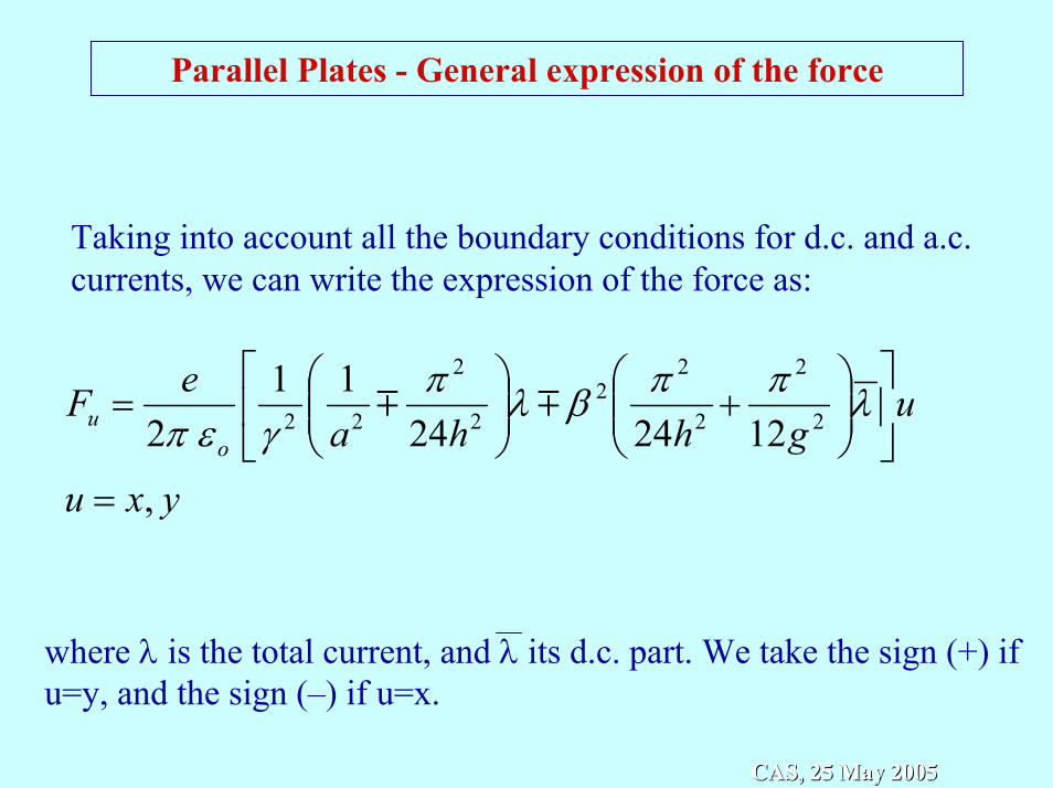
Parallel Plates - General expression of the force

Taking into account all the boundary conditions for d.c. and a.c. currents, we can write the expression of the force as:

yxu

ughha

eFo

u

,

12242411

2 2

2

2

22

2

2

22

=

+

= λππβλπ

γεπmm

where λ is the total current, and λ its d.c. part. We take the sign (+) if u=y, and the sign (–) if u=x.

CAS, 25 May 2005CAS, 25 May 2005

Space charge effects in storage rings

CAS, 25 May 2005CAS, 25 May 2005

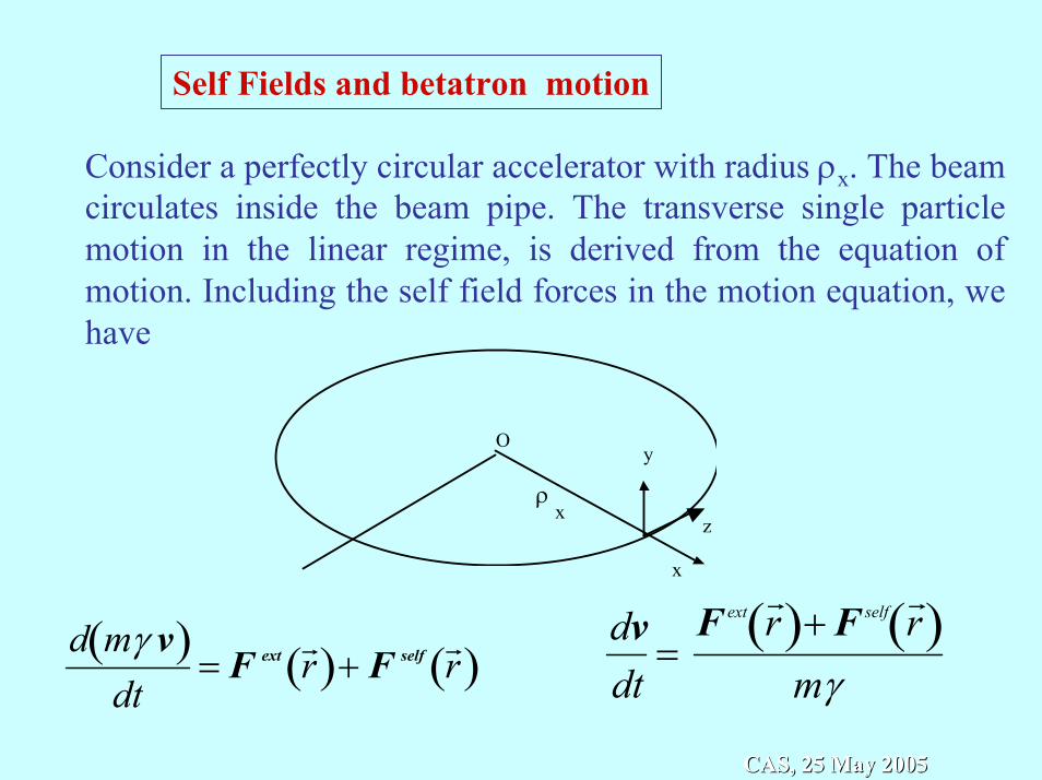
Self Fields and betatron motion

Consider a perfectly circular accelerator with radius ρx. The beam circulates inside the beam pipe. The transverse single particle motion in the linear regime, is derived from the equation of motion. Including the self field forces in the motion equation, we have

d mγ v( )

dt= F ext r

r ( )+ F self r r ( )

O

ρx

y

x

z

dvdt

=F ext r

r ( )+ F self r r ( )

mγ

CAS, 25 May 2005CAS, 25 May 2005

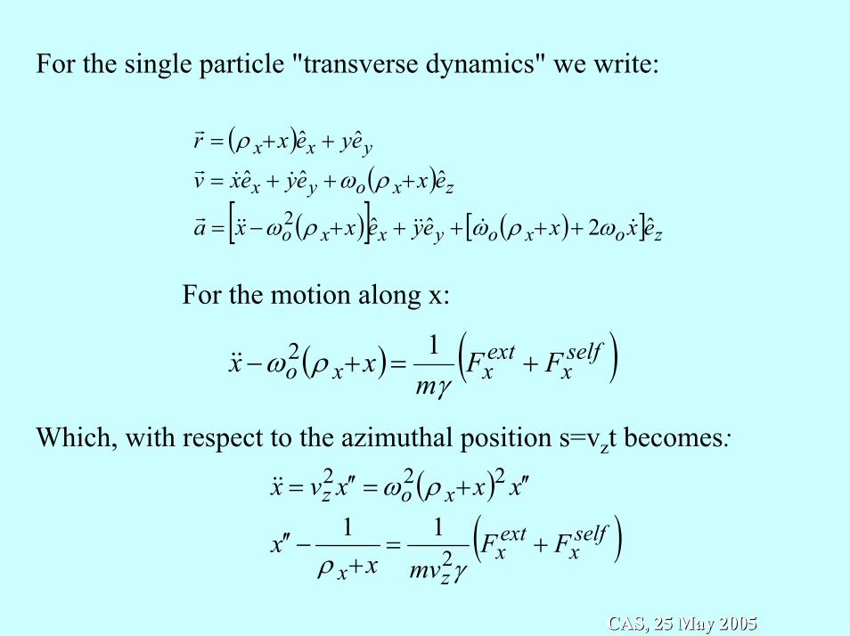
For the single particle "transverse dynamics" we write:

( )( )

( )[ ] ( )[ ] zoxoyxxo

zxoyx

yxx

exxeyexxa

exeyexv

eyexr

ˆ2ˆˆ

ˆˆˆ

ˆˆ

2 &&&&&&r

&&r

r

ωρωρω

ρω

ρ

+++++−=

+++=

++=

For the motion along x:

( ) ( )selfx

extxxo FF

mxx +=+−

γρω 12&&

Which, with respect to the azimuthal position s=vzt becomes:

( )

( )selfx

extx

zx

xoz

FFmvx

x

xxxvx

+=+

−′′

′′+=′′=

γρ

ρω

2

222

11&&

CAS, 25 May 2005CAS, 25 May 2005

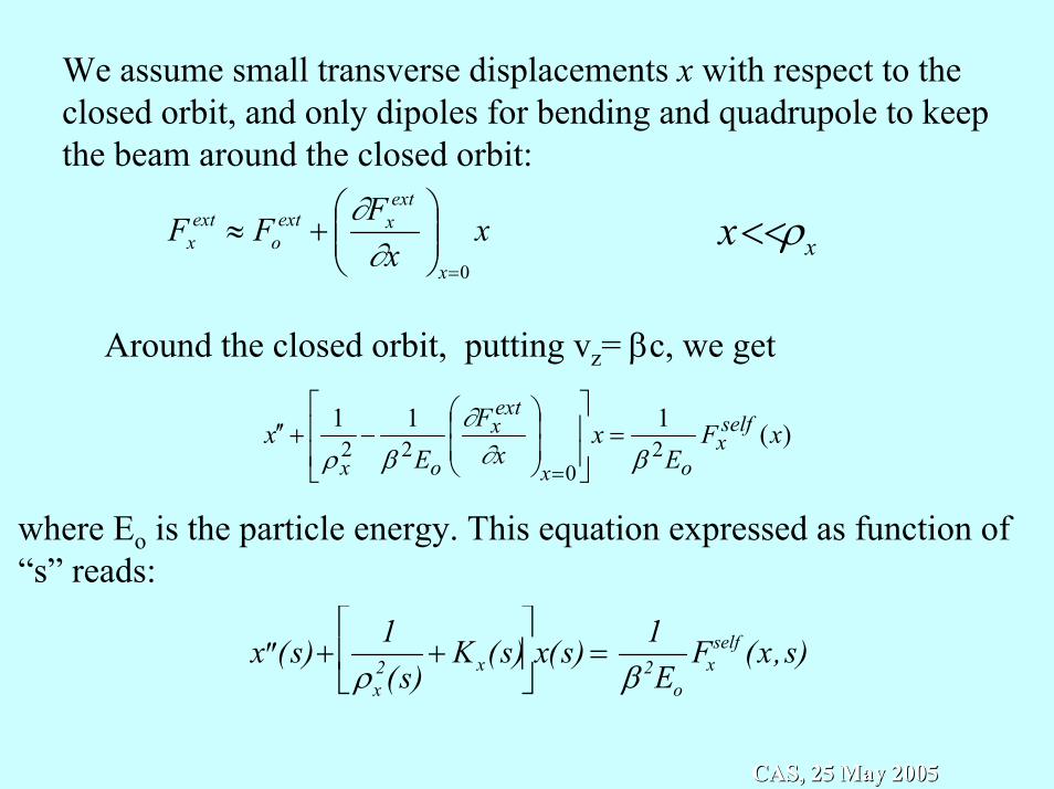
We assume small transverse displacements x with respect to the closed orbit, and only dipoles for bending and quadrupole to keep the beam around the closed orbit:

xx

FFFx

extxext

oext

x0=

+≈

∂∂ x<<ρx

Around the closed orbit, putting vz= βc, we get

)(1112

022 xF

Ex

xF

Ex self

xox

extx

ox β∂∂

βρ=

−+′′

=

where Eo is the particle energy. This equation expressed as function of “s” reads:

′ ′ x (s)+1

ρx2(s)

+ Kx(s)

x(s) =

1β 2Eo

Fxself (x,s)

CAS, 25 May 2005CAS, 25 May 2005

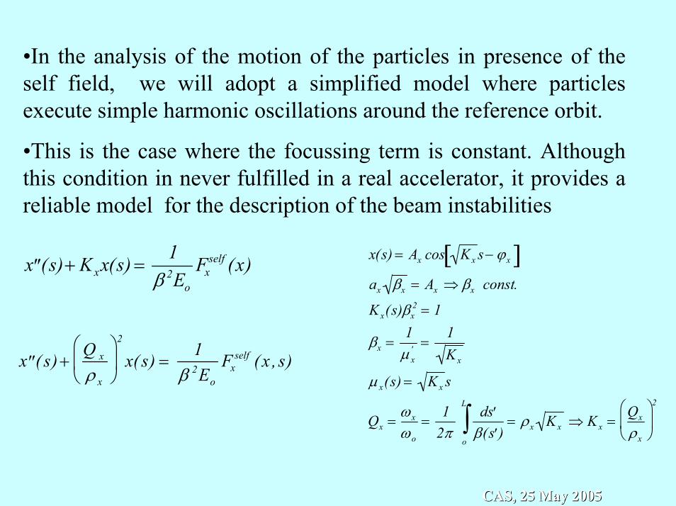
•In the analysis of the motion of the particles in presence of the self field, we will adopt a simplified model where particles execute simple harmonic oscillations around the reference orbit.

•This is the case where the focussing term is constant. Although this condition in never fulfilled in a real accelerator, it provides a reliable model for the description of the beam instabilities

x(s) = Ax cos Kx s− ϕx[ ]ax βx = Ax ⇒ βx const.

Kx(s)βx2 = 1

βx =1

µ x' =

1Kx

µ x(s) = Kx s

Qx =ωx

ωo

=1

2πd ′ s

β( ′ s )o

L

∫ = ρx Kx ⇒ Kx =Qx

ρx

2

′ ′ x (s)+ Kxx(s) =1

β 2Eo

Fxself (x)

′ ′ x ( s) +Q x

ρ x

2

x( s) =1

β 2Eo

Fxself ( x , s)

CAS, 25 May 2005CAS, 25 May 2005

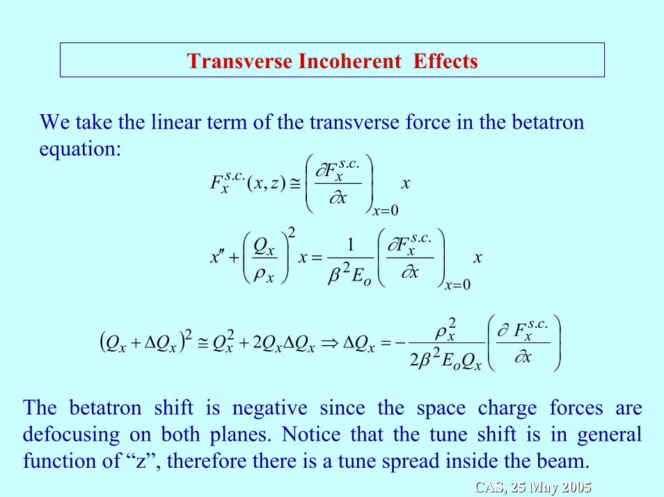
Transverse Incoherent Effects

We take the linear term of the transverse force in the betatronequation:

xx

FE

xQx

xx

FzxF

x

csx

ox

x

x

csxcs

x

0

..

2

20

....

1

),(

=

=

=

+′′

≅

∂∂

βρ

∂∂

( )

−=∆⇒∆+≅∆+

xF

QEQQQQQQ

csx

xo

xxxxxxx ∂

∂β

ρ ..

2

222

22

The betatron shift is negative since the space charge forces are defocusing on both planes. Notice that the tune shift is in general function of “z”, therefore there is a tune spread inside the beam.

CAS, 25 May 2005CAS, 25 May 2005

Consequences of the space charge tune shifts

In circular accelerators the values of the betatron tunes should not be close to rational numbers in order to avoid the crossing of linear and non-linear resonances where the beam becomes unstable.

The tune spread induced by the space charge force can make hard to satisfy this basic requirement. Typically, in order to avoid major resonances the stability requires

3.0<∆ uQ

CAS, 25 May 2005CAS, 25 May 2005

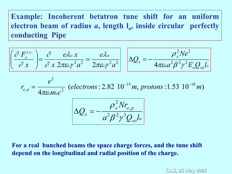
oxooo

xx lQEa

NeQ 222

22

4 γβπερ

−=∆

Example: Incoherent betatron tune shift for an uniform electron beam of radius a, length lo, inside circular perfectly conducting Pipe

2222

..

2

2

ae

axe

xxF

o

o

o

ocs

x

γπελ

γπελ

∂∂

∂∂

==

)01 53.1 : ,01 82.2:( 4

18152

2

, mprotonsmelectronscm

er

oope

−−=πε

oxo

pexx lQa

NrQ 322

,2

γβρ

−=∆

For a real bunched beams the space charge forces, and the tune shift depend on the longitudinal and radial position of the charge.

CAS, 25 May 2005CAS, 25 May 2005

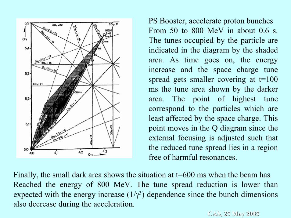
PS Booster, accelerate proton bunchesFrom 50 to 800 MeV in about 0.6 s. The tunes occupied by the particle are indicated in the diagram by the shaded area. As time goes on, the energy increase and the space charge tune spread gets smaller covering at t=100 ms the tune area shown by the darker area. The point of highest tune correspond to the particles which are least affected by the space charge. This point moves in the Q diagram since the external focusing is adjusted such that the reduced tune spread lies in a region free of harmful resonances.

Finally, the small dark area shows the situation at t=600 ms when the beam hasReached the energy of 800 MeV. The tune spread reduction is lower than expected with the energy increase (1/γ3) dependence since the bunch dimensions also decrease during the acceleration.

CAS, 25 May 2005CAS, 25 May 2005

END

CAS, 25 May 2005CAS, 25 May 2005