Solutions to Problems for Infinite Spatial Domain

and the Fourier Transform

18.303 Linear Partial Differential Equations

Matthew J. Hancock

Fall 2004

1 Problem 1

(i) Show that

u (x, t) = u0erf

(x

2√

t

), t > 0, x ∈ R, (1)

where u0 is a constant, is a solution of the heat equation

ut = uxx, (2)

and satisfies the initial condition

u (x, 0) = f (x) =

u0, if x > 0,

0, if x = 0,

−u0, if x < 0

(3)

in the sense that

limt→0+

u (x, t) = f (x) .

Solution: We show by direct substitution that u (x, t) is the solution to the heat

equation and initial condition. First, note that the error function is defined by

erf (x) =2√π

∫ x

0

e−s2

ds (4)

1

Thus by the chain rule,

ut = u02√π

exp

(−x2

4t

)x

2t3/2

(−1

2

)= − u0x

2√

πt3/2exp

(−x2

4t

)

uxx =∂2

∂x2

(u0erf

(x

2√

t

))=

∂

∂x

(u0

2√π

1

2√

texp

(−x2

4t

))

= u02√π

exp

(−x2

4t

)1

2√

t

(−2x

4t

)

= − u0x

2√

πt3/2exp

(−x2

4t

)= ut

Thus Eq. (1) for u (x, t) satisfies the Heat Equation (2).

We now show that (1) satisfies the IC (3). Note that

x > 0 : limt→0+

u (x, t) = u0erf

(lim

t→0+

x

2√

t

)= u0erf (∞) = u0

x = 0 : limt→0+

u (0, t) = limt→0+

0 = 0

x < 0 : limt→0+

u (x, t) = u0erf

(lim

t→0+

x

2√

t

)= u0erf (−∞) = −u0

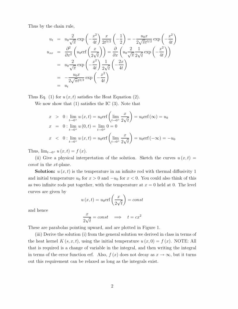
Thus, limt→0+ u (x, t) = f (x).

(ii) Give a physical interpretation of the solution. Sketch the curves u (x, t) =

const in the xt-plane.

Solution: u (x, t) is the temperature in an infinite rod with thermal diffusivity 1

and initial temperature u0 for x > 0 and −u0 for x < 0. You could also think of this

as two infinite rods put together, with the temperature at x = 0 held at 0. The level

curves are given by

u (x, t) = u0erf

(x

2√

t

)= const

and hencex

2√

t= const =⇒ t = cx2

These are parabolas pointing upward, and are plotted in Figure 1.

(iii) Derive the solution (i) from the general solution we derived in class in terms of

the heat kernel K (s, x, t), using the initial temperature u (x, 0) = f (x). NOTE: All

that is required is a change of variable in the integral, and then writing the integral

in terms of the error function erf. Also, f (x) does not decay as x → ∞, but it turns

out this requirement can be relaxed as long as the integrals exist.

2

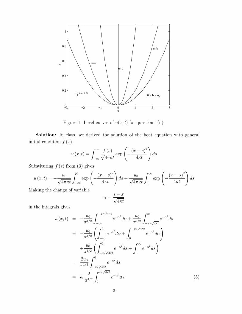
−3 −2 −1 0 1 2 30

0.2

0.4

0.6

0.8

1

x

t

−u0< a < 0

u=a

u=0

u=b

0 < b < u0

Figure 1: Level curves of u(x, t) for question 1(ii).

Solution: In class, we derived the solution of the heat equation with general

initial condition f (x),

u (x, t) =

∫ ∞

−∞

f (s)√4πκt

exp

(−(x − s)2

4κt

)ds

Substituting f (s) from (3) gives

u (x, t) = − u0√4πκt

∫ 0

−∞exp

(−(x − s)2

4κt

)ds +

u0√4πκt

∫ ∞

0

exp

(−(x − s)2

4κt

)ds

Making the change of variable

α =s − x√

4κtin the integrals gives

u (x, t) = − u0

π1/2

∫ −x/√

4κt

−∞e−α2

dα +u0

π1/2

∫ ∞

−x/√

4κt

e−α2

ds

= − u0

π1/2

(∫ 0

−∞e−α2

dα +

∫ −x/√

4κt

0

e−α2

dα

)

+u0

π1/2

(∫ 0

−x/√

4κt

e−α2

ds +

∫ ∞

0

e−α2

ds

)

=2u0

π1/2

∫ 0

−x/√

4κt

e−α2

ds

= u02

π1/2

∫ x/√

4κt

0

e−α2

ds (5)

3

since ∫ 0

−∞e−α2

dα =

∫ ∞

0

e−α2

ds.

Substituting the definition of the error function (4) into (5) and setting κ = 1 gives

u (x, t) = u0erf

(x

2√

t

)

as required.

2 Problem 2

(i) Find the temperature u (x, t) of a semi-infinite rod (x ≥ 0), whose end (x = 0) is

kept at a temperature of zero, and with an initial hot-spot, u (x, 0) = f (x), where

f (x) =

{u0, if x ∈ (x0, x1)

0, if x ∈ [0, x0) ∪ (x1,∞)(6)

with x0, x1 constants, 0 ≤ x0 < x1. Sketch the temperature profiles t = const (i.e.,

u (x, t0) in the ux-plane for various fixed times t0), x = const (i.e., u (x0, t) in the

ut-plane for various fixed x0) and the level curves u (x, t) = const in the xt-plane. See

note below.

(ii) Repeat (i) with the end of the rod (x = 0) insulated. See note below.

(iii) Referring to (ii), show that the temperature of the insulated end is a maximum

at time

t =x2

1 − x20

4κ (log x1 − log x0)

where κ is the thermal diffusivity.

NOTE: in both (i) and (ii), just use the general solution we derived in class with

the heat kernel, by suitably extending f (x) to the whole real line (i.e. odd extension

or even extension - see class notes). The integrals in the solution can then be expressed

as the sum of four terms involving error functions erf.

Solution (i): In class, we derived that solution to the heat equation on a semi-

infinite rod (x ≥ 0) whose end is kept at zero is

u (x, t) =

∫ ∞

−∞

f̃ (s)√4πκt

exp

(−(x − s)2

4κt

)ds (7)

where f̃ (s) is the odd extension of f (s),

f̃ (s) =

f (s) , s > 0

0, s = 0

−f (−s) , s < 0

(8)

4

Substituting (8) into (7) gives

u (x, t) = −∫ 0

−∞

f (−s)√4πκt

exp

(−(x − s)2

4κt

)ds +

∫ ∞

0

f (s)√4πκt

exp

(−(x − s)2

4κt

)ds

Substituting for f (s) from (6) gives

u (x, t) = − u0√4πκt

∫ −x0

−x1

exp

(−(x − s)2

4κt

)ds +

u0√4πκt

∫ x1

x0

exp

(−(x − s)2

4κt

)ds

Making the change of variable

α =s − x√

4κt

gives

u (x, t) = − u0√π

∫ −x0−x√4κt

−x1−x√4κt

e−α2

dα +u0√π

∫ x1−x√4κt

x0−x√4κt

e−α2

dα

=u0√π

(−∫ 0

−x1−x√4κt

e−α2

dα −∫ −x0−x√

4κt

0

e−α2

dα +

∫ 0

x0−x√4κt

e−α2

dα +

∫ x1−x√4κt

0

e−α2

dα

)

=u0√π

(−∫ x1+x√

4κt

0

e−α2

dα +

∫ x0+x√4κt

0

e−α2

dα −∫ x0−x√

4κt

0

e−α2

dα +

∫ x1−x√4κt

0

e−α2

dα

)

Substituting the definition of the error function (4) gives

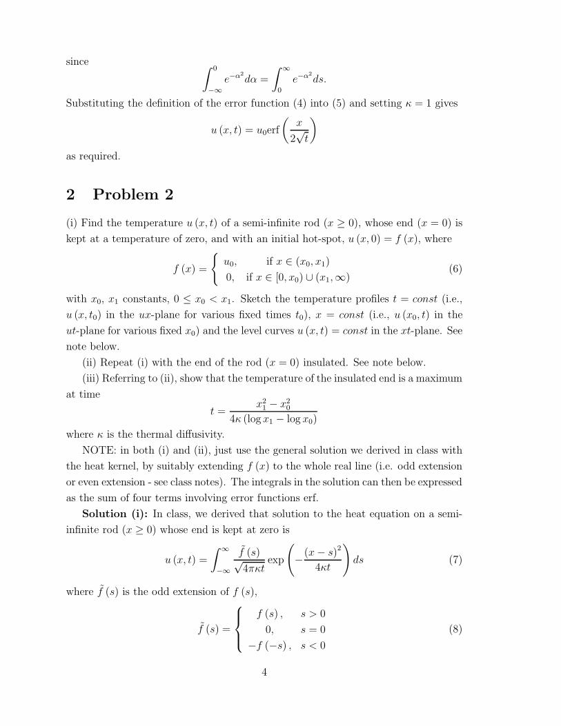
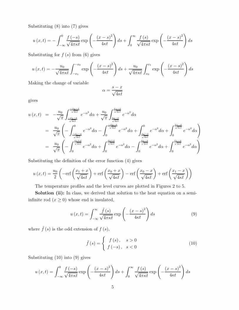
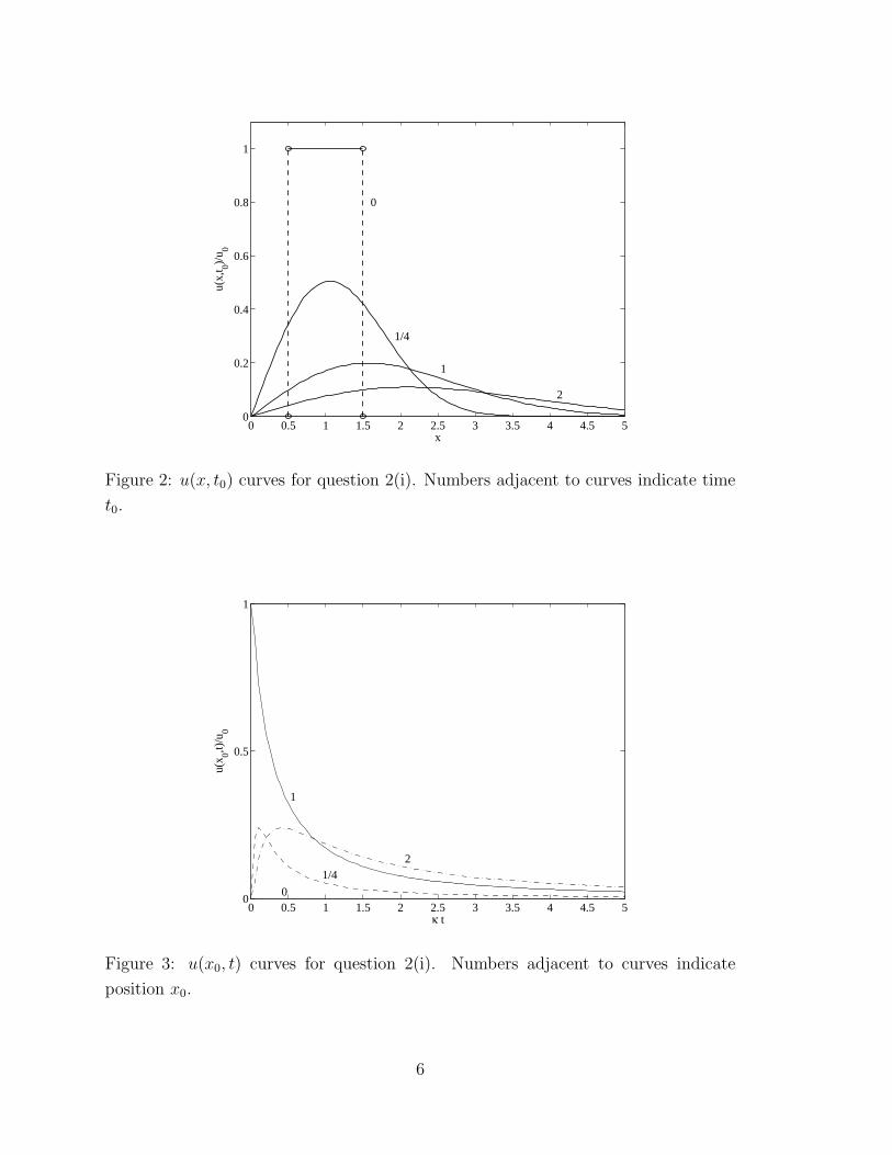
u (x, t) =u0

2

(−erf

(x1 + x√

4κt

)+ erf

(x0 + x√

4κt

)− erf

(x0 − x√

4κt

)+ erf

(x1 − x√

4κt

))

The temperature profiles and the level curves are plotted in Figures 2 to 5.

Solution (ii): In class, we derived that solution to the heat equation on a semi-

infinite rod (x ≥ 0) whose end is insulated,

u (x, t) =

∫ ∞

−∞

f̃ (s)√4πκt

exp

(−(x − s)2

4κt

)ds (9)

where f̃ (s) is the odd extension of f (s),

f̃ (s) =

{f (s) , s > 0

f (−s) , s < 0(10)

Substituting (10) into (9) gives

u (x, t) =

∫ 0

−∞

f (−s)√4πκt

exp

(−(x − s)2

4κt

)ds +

∫ ∞

0

f (s)√4πκt

exp

(−(x − s)2

4κt

)ds

5

0 0.5 1 1.5 2 2.5 3 3.5 4 4.5 50

0.2

0.4

0.6

0.8

1

0

1/4

1

2

x

u(x,

t 0)/u 0

Figure 2: u(x, t0) curves for question 2(i). Numbers adjacent to curves indicate time

t0.

0 0.5 1 1.5 2 2.5 3 3.5 4 4.5 50

0.5

1

0

1/4

1

2

κ t

u(x 0,t)

/u0

Figure 3: u(x0, t) curves for question 2(i). Numbers adjacent to curves indicate

position x0.

6

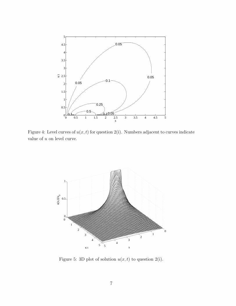
0 0.5 1 1.5 2 2.5 3 3.5 4 4.5 50

0.5

1

1.5

2

2.5

3

3.5

4

4.5

5

x

κ t

0.5

0.25

0.1

0.1

0.1

0.05

0.05

0.05

0.05

Figure 4: Level curves of u(x, t) for question 2(i). Numbers adjacent to curves indicate

value of u on level curve.

01

23

45

0

1

2

3

4

5

0

0.5

1

xκ t

u(x,

t)/u

0

Figure 5: 3D plot of solution u(x, t) to question 2(i).

7

0 0.5 1 1.5 2 2.5 3 3.5 4 4.5 50

0.2

0.4

0.6

0.8

1

0

1/4 12

x

u(x,

t 0)/u 0

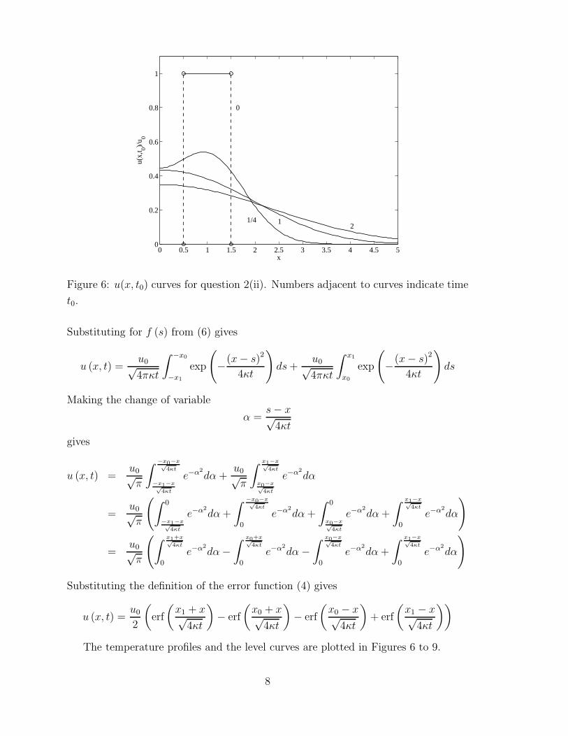
Figure 6: u(x, t0) curves for question 2(ii). Numbers adjacent to curves indicate time

t0.

Substituting for f (s) from (6) gives

u (x, t) =u0√4πκt

∫ −x0

−x1

exp

(−(x − s)2

4κt

)ds +

u0√4πκt

∫ x1

x0

exp

(−(x − s)2

4κt

)ds

Making the change of variable

α =s − x√

4κt

gives

u (x, t) =u0√π

∫ −x0−x√4κt

−x1−x√4κt

e−α2

dα +u0√π

∫ x1−x√4κt

x0−x√4κt

e−α2

dα

=u0√π

(∫ 0

−x1−x√4κt

e−α2

dα +

∫ −x0−x√4κt

0

e−α2

dα +

∫ 0

x0−x√4κt

e−α2

dα +

∫ x1−x√4κt

0

e−α2

dα

)

=u0√π

(∫ x1+x√4κt

0

e−α2

dα −∫ x0+x√

4κt

0

e−α2

dα −∫ x0−x√

4κt

0

e−α2

dα +

∫ x1−x√4κt

0

e−α2

dα

)

Substituting the definition of the error function (4) gives

u (x, t) =u0

2

(erf

(x1 + x√

4κt

)− erf

(x0 + x√

4κt

)− erf

(x0 − x√

4κt

)+ erf

(x1 − x√

4κt

))

The temperature profiles and the level curves are plotted in Figures 6 to 9.

8

0 0.5 1 1.5 2 2.5 3 3.5 4 4.5 50

0.1

0.2

0.3

0.4

0.5

0.6

0.7

0.8

0.9

1

0

1/4

1

2

κ t

u(x 0,t)

/u0

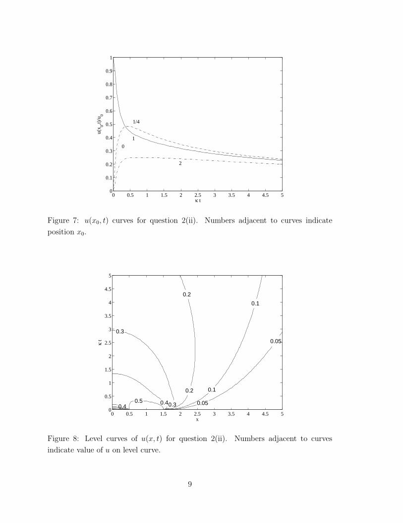
Figure 7: u(x0, t) curves for question 2(ii). Numbers adjacent to curves indicate

position x0.

0 0.5 1 1.5 2 2.5 3 3.5 4 4.5 50

0.5

1

1.5

2

2.5

3

3.5

4

4.5

5

x

κ t

0.50.4

0.40.3

0.3

0.2

0.2

0.1

0.1

0.05

0.05

Figure 8: Level curves of u(x, t) for question 2(ii). Numbers adjacent to curves

indicate value of u on level curve.

9

01

23

45

0

1

2

3

4

5

0

0.2

0.4

0.6

0.8

1

xκ t

u(x,

t)/u

0

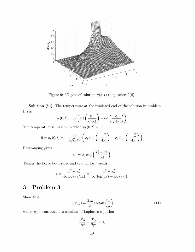
Figure 9: 3D plot of solution u(x, t) to question 2(ii).

Solution (iii): The temperature at the insulated end of the solution in problem

(ii) is

u (0, t) = u0

(erf

(x1√4κt

)− erf

(x0√4κt

))The temperature is maximum when ut (0, t) = 0,

0 = ut (0, t) = − u0

4√

κt3/2

(x1 exp

(− x2

1

4κt

)− x0 exp

(− x2

0

4κt

))

Rearranging gives

x1 = x0 exp

(x2

1 − x20

4κt

)Taking the log of both sides and solving for t yields

t =x2

1 − x20

4κ log (x1/x0)=

x21 − x2

0

4κ (log (x1) − log (x0))

3 Problem 3

Show that

u (x, y) =2u0

πarctan

(x

y

)(11)

where u0 is constant, is a solution of Laplace’s equation

∂2u

∂x2+

∂2u

∂y2= 0,

10

and satisfies the boundary condition

limy→0+

u (x, y) = f (x)

Give a physical interpretation of the solution (i.e. how does this relate to what

Heat Problem?). Sketch the isothermal curves (level curves) u (x, y) = const in the

xy-plane. Note that in polar coordinates,

θ = arctan

(x

y

)

where θ is the angle measured from the y-axis (θ = 0 is the y-axis) and increasing

clockwise.

Solution: We can show u (x, y) is a solution of Laplace’s equation directly,

∂u

∂x=

2u0

π

1

1 + (x/y)2

1

y,

∂2u

∂x2= −2u0

π

2xy

(y2 + x2)2

∂u

∂y=

2u0

π

1

1 + (x/y)2

−x

y2,

∂2u

∂y2=

2u0

π

2xy

(y2 + x2)2

Thus∂2u

∂x2+

∂2u

∂y2= −2u0

π

2xy

(y2 + x2)2 +2u0

π

2xy

(y2 + x2)2 = 0

and hence (11) is a solution of Laplace’s equation. The limit y → 0+ of (11) is

x > 0 : limy→0+

u (x, y) =2u0

πlim

y→0+arctan

(x

y

)=

2u0

πarctan (∞) =

2u0

π

π

2= u0

x = 0 : limy→0+

u (0, y) =2u0

πlim

y→0+0 = 0

x < 0 : limy→0+

u (x, y) =2u0

πlim

y→0+arctan

(x

y

)=

2u0

πarctan (−∞) = −2u0

π

π

2= −u0

Thus

limy→0+

u (x, y) = f (x)

where f (x) is given in (3) in problem 1.

We can also show that (11) is a solution of Laplace’s equation by substituting

f (s) into the general solution we derived in class using the Fourier Transform,

u (x, y) =1

2π

∫ ∞

−∞f (s)

2y

(x − s)2 + y2ds

=1

2π

(∫ 0

−∞f (s)

2y

(x − s)2 + y2ds +

∫ ∞

0

f (s)2y

(x − s)2 + y2ds

)

=yu0

π

(−∫ 0

−∞

ds

(x − s)2 + y2+

∫ ∞

0

ds

(x − s)2 + y2

)

11

Note that ∫ b

a

ds

(s − x)2 + y2=

∫ b−x

a−x

dα

α2 + y2=

[1

yarctan

(α

y

)]b−x

α=a−x

=1

yarctan

(b − x

y

)− 1

yarctan

(a − x

y

)

Thus

u (x, y) =yu0

π

(−1

yarctan

(−x

y

)+

1

yarctan

(−∞− x

y

))

+yu0

π

(1

yarctan

(∞− x

y

)− 1

yarctan

(−x

y

))

=u0

π

(2 arctan

(x

y

)− π

2+

π

2

)

=2u0

πarctan

(x

y

)

as required.

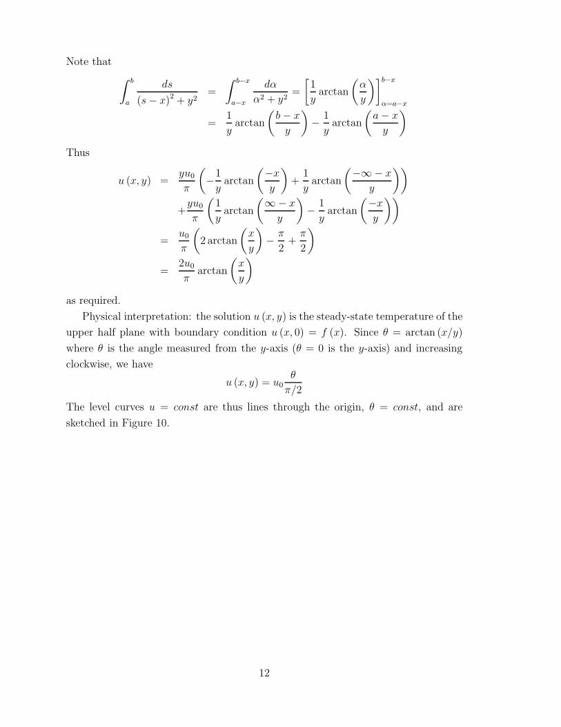
Physical interpretation: the solution u (x, y) is the steady-state temperature of the

upper half plane with boundary condition u (x, 0) = f (x). Since θ = arctan (x/y)

where θ is the angle measured from the y-axis (θ = 0 is the y-axis) and increasing

clockwise, we have

u (x, y) = u0θ

π/2

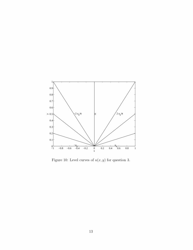
The level curves u = const are thus lines through the origin, θ = const, and are

sketched in Figure 10.

12

−1 −0.8 −0.6 −0.4 −0.2 0 0.2 0.4 0.6 0.8 10

0.1

0.2

0.3

0.4

0.5

0.6

0.7

0.8

0.9

1

x

y 0

u0

−u0

2 u0/π−2 u

0/π

Figure 10: Level curves of u(x, y) for question 3.

13