κ-Solutions Of the Ricci Flow ∗

Rugang YeDepartment of Mathematics

University of California, Santa Barbara

December 10, 2007

Abstract: The concept of κ-solutions of the Ricci flow plays an important role inPerelman’s work on the Ricci flow, the Poincare conjecture and the geometrizationconjecture. In this paper we present a number of results on κ-solutions and a concisepicture of this role .

Table of contents1. Introduction2. Blow-up limits of the Ricci flow and κ-solutions3. Asymptotical solitons, the l-function and the reduced volume4. Classification of 2-dimensional κ-solutions5. Classification of 3-dimensional κ-solutions and Perelman’s compactness theorem6. Achieving bounded curvature and the canonical neighborhood theorem

1 Introduction

Let M be a smooth manifold of dimension n ≥ 2. The Ricci flow

∂g

∂t= −2Ric (1.1)

was introduced by R. Hamilton in his seminar paper [H1] on 3-dimensional manifoldsof positive Ricci curvature. Here, g = g(t) is a smooth family of Riemannian metricson M and Ric the Ricci curvature tensor of g = g(t). (For basics and generalinformation on the Ricci flow we refer to [H1], [H5], [CK] and [CLN].) The conceptof κ-solutions of the Ricci flow was introduced by G. Perelman in his seminar papers[P1] and [P2], and plays a crucial role in the analysis of the structures of blow-up singularities of the Ricci flow, and thereby a crucial role in Perelman’s work in

∗2000 Mathematics Subject Classification: 53C20, 53C21

1

[P1],[P2] and [P3] on Poincare conjecture and Thurston’s geometrization conjecture on3-dimensional manifolds. See Section 1 for the definition of this concept. (Perelman’sterminology for this concept is ancient κ-solutions.) In the Ricci flow approach tothe Poincare conjecture and the geometrization conjecture, which was initiated byHamilton, one chooses a Riemannian metric g0 on an arbitrary compact 3-dimensionalmanifold M and considers the smooth solution g = g(t) of the Ricci flow (1.1) withinitial value g(0) = g0. This smooth solution exists on a maximal time interval [0, T ),where T can be finite or infinite. Without special geometric conditions on g0, ingeneral one expects T to be finite. If one chooses a reference point p ∈ M for thepurpose of measuring geometric quantities with respect to distance from p, then wehave a pointed Ricci flow (g = g(t),M × [0, T ), p). Assume T < ∞. As t → T , theRicci flow g(t) will blow up, i.e. the norm of the Riemann curvature tensor |Rm| willbecome infinite at least in some places of M . In order to gain information on thegeometric and topological structures of the manifold M , it is crucial to analyze thestructures of the blow singularities of the flow g(t) as t→ T .

A general method for carrying out this analysis is to rescale the Ricci flow g(t)and obtain blow-up limits from g(t). Let’s consider the general case n ≥ 3. For apositive number λ and a number T ∈ (0, T ), the rescaled flow gλ,T (t) with scalingfactor λ and scaling center time T is defined to be

gλ,T (t) = λg(T + λ−1t) (1.2)

for t ∈ [−λT , λ(T − T )). By the scaling invariance of the Ricci flow, gλ,T is a smoothsolution of the Ricci flow on M . For a sequence of scaling factors λk → ∞ andscaling center times Tk, we have a sequence of rescaled Ricci flows gk = gλk,Tk . Ifwe also choose a sequence of reference points pk, then we have a sequence of pointedRicci flows (gk,M × [−λTk, λk(T − Tk)), pk). Now the basic idea is to choose λk, Tkand pk suitably such that we can extract from this sequence of pointed Ricci flowssubsequences which point converge (i.e. converge smoothly with the reference pointspk as centers) to smooth limits, which are called blow-up limits. These limits arepointed Ricci flows on limit manifolds with limit reference points, which we denoteby (g∞,M∞×(−∞, 0], p∞). They are ancient solutions of the Ricci flow, namely theyare defined on the time interval (−∞, 0] and consist of complete Riemannian metrics.Moreover, they enjoy some special geometric properties.

In dimension n = 3, the blow-up limits turn out to be κ-solutions. Since theyarise as blow-up limits of the Ricci flow g = g(t), they model the structures of theblow-up singularities of g = g(t) (as t → T ). Indeed, the results in [P1] and [P2]on structures of blow-up singularities of the Ricci flow are deduced by employing thespecial geometric and topological properties of κ-solutions. In the above account weassumed T <∞. The general arguments of blow-up analysis as described above alsowork in the case T = ∞, with a major difference between T < ∞ and T = ∞.Namely, in the case T <∞, the Ricci flow g = g(t) is always κ-noncollapsed. In thecase T =∞, it may collapse as t→ T , and hence the rescaled flows may degenerate to

2

lower dimensional objects. For this reason, the blow-up analysis is more complicatedin the case T =∞. Fortunately, Perelman’s solution of the Poincare conjecture andthe geometrization conjecture do not require analysis of blow-up limits for T =∞ inthe collapsing case.

Once the structures of the blow-up singularities as t → T are well-understood,namely their topological and geometric types are classified and well under control, aspresented in [P1] and [P2], one can perform surgery at t = T to remove singularitiesand construct a manifold M with surgery out of M and a metric g with surgery out ofa partial limit of g at T , as done in [P2]. (Earlier work on surgeries of the Ricci flowwas done by Hamilton [H8].) Then one considers the Ricci flow on M with the initialmetric g. If g runs into blow-up singularities at some finite time, the above blow-upanalysis can be repeated for g. By induction, one then obtains a Ricci flow g∗ = g∗(t)with surgeries which consists of a sequence of smooth solutions of the Ricci flow on asequence of smooth manifolds, as done in [P2]. This Ricci flow with surgeries existson a maximal time interval [0, T ∗). An important special case is included in thisscheme. If the Ricci flow g = g(t) blows up on the whole M as t → ∞, then thereis nothing left from M for performing surgery. In this case, the topological structureof M is immediately classified in consistence with the Poincare conjecture. The samekind of picture can also occur at a later stage of the Ricci flow g∗ with surgeries. Ineither case, the Ricci flow with surgeries g∗ is said to be extinct (at a finite time), andthe goal of classifying the topological structure of M is achieved. For convenience,we extend g∗ to be the empty solution on [T ,∞) if T is an extinction time. By anintricate argument, Perelman shows that in general T ∗ =∞ (without assuming finitetime extinction), see [P2] and the expositions in [MT] and [KL].

The next stage of Perelman’s work goes as follows. On the one hand, he showsin [P3] that under the condition of the Poincare conjecture, g∗ has to be extinct ata finite time (see also [CM]). This leads to his proof of the Poincare conjecture aspresented in [P2] and [P3]. On the other hand, in the general situation he shows in[P2] that as t → ∞, the Ricci flow with surgeries g∗ leads to the geometrization ofM , i.e. a suitable decomposition of M into finite many pieces, such that each piececarries a standard geometric structure. This includes the Poincare conjecture as aspecial case. Here Perelman applies an important argument of Hamilton in [H8] forobtaining hyperbolic manifolds as limits as t→∞ from the noncollapsing part of theRicci flow, and appeals to his own results on locally collapsing manifolds for obtainingthe desired topological and geometric structures on the collapsing part of the Ricciflow. (See [SY] for relevant results on collapsed manifolds.)

It should be clear from the above accounts that κ-solutions play a crucial rolein Perelman’s work. Although Perelman only needs the case n = 3, the prospect ofapplying the Ricci flow in higher dimensions looks promising, and hence it is of greatinterests to understand κ-solutions also in higher dimensions. Indeed, many resultsof Perelman on κ-solutions are valid in general dimensions.

The contents of this paper are organized as follows. In Section 1, we present the

3

concept of κ-noncollpasedness, a basic result on blow-up limits of the Ricci flow andthe concept of κ-solutions. In Section 2, we present the concept of gradient shrinkingsolitons and Perelman’s theorem on gradient shrinking solitons as blow-down limitsof κ-solutions, which plays an important role for understanding the structures of κ-solutions. In [P1], a sketch of the proof for this theorem was given. The completeproof of this theorem was presented in the author’s papers [Y2] and [Y3] (see also[MT] and [KL]). In this section, two important tools, the l-function (the reducedlength) and the reduced volume, are also presented. In Section 3, we present theclassification of 2-dimensional κ-solutions. This result is crucial for carrying out theargument of dimension reduction, in which a 3-dimensional Ricci flow splits into theproduct of a 2-dimensional Ricci flow with the 1-dimensional Ricci flow. This argu-ment plays an important role in a number of places, e.g. in classifying 3-dimensionalκ-solutions. The proof of the classification of 2-dimensional κ-solutions presented in[P1] is incomplete. The first complete proof was given in the author’s paper [Y4].This proof is reproduced here. (The proof in [Y4] was later adapted in [CZ]. Differentarguments were presented in [KL] and [MT].) In Section 4, we present Perelman’sclassification of 3-dimensional κ-solutions and his compactness theorem for the spaceof 3-dimensional noncompact κ-solutions. In Section 5, we present Perelman’s the-orem on canonical neighborhoods of solutions of the Ricci flow, which is a central,culminating result. By using this result we demonstrate that the blow-up limits(g∞,M∞× (−∞, 0], p∞) discussed above must be κ-solutions in dimension 3. We alsopresent Perelman’s result on obtaining bounded curvature at bounded distance anda result on obtaining suitable scaling parameters (λk, Tk, pk) as discussed above suchthat the blow-up sequence gk subconverges.

Our goal is to present a concise picture of the theory of κ-solutions and its role inPerelman’s work on the Ricci flow, the Poincare conjecture and the geometrizationconjecture. We do not attempt to include all results on κ-solutions. In a number ofplaces we stay away from complicated technical details of the proofs. The completedetails can be found in Perelman’s papers [P1] and [P2], the excellent book [MT]and notes [KL], the paper [CZ], and the papers [Y1], [Y2], [Y3], [Y4] and [Y5]. (Thespecific references are always given.) On the other hand, we include complete proofsin a number of other places, e.g. in Section 4, because these proofs are relativelyshort and can provide a good help for understanding the concepts and methods, orbecause we cannot find suitable references for the complete details.

2 Blow-up limits of the Ricci flow and κ-solutions

Definition 1 ([P1]) Let (M, g) be a complete Riemannian manifold of dimensionn ≥ 1. Consider positive numbers κ and ρ. We say that (M, g) is κ-noncollapsed onthe scale ρ, provided that every geodesic ball B(x, r) of radius r < ρ in (M, g), onwhich |Rm| ≤ r−2 holds, has volume at least κrn.

4

Definition 2 ([P1]) A κ-solution (of the Ricci flow (1.1)) is an ancient nonflat so-lution of the Ricci flow (1.1) on a manifold M with bounded nonnegative curvatureoperator which is κ-noncollapsed for some κ > 0 on all scales. More precisely, aκ-solution is a smooth solution g = g(t) of the Ricci flow for −∞ < t ≤ 0 on somemanifold M such that for each t, the metric g(t) is complete, nonflat, has boundedand nonnegative curvature operator, and is κ-noncollapsed on all scales.

Round spheres give rise to obvious examples of κ-solutions. Consider the sphereSn, n ≥ 1. Let g0 denote a constant multiple of the standand round sphere metricgSn of sectional curvature 1 on Sn. Then g(t) = (1 − 2

nRg0t)g0, t ∈ (−∞, 0] is a κ-

solution on Sn, where Rg0 denotes the scalar curvature of g0. In dimension 2, we haveκ = 8π(1− cos 1√

2). If M is a manifold diffeomorphic to Sn, we can pull back g to M

by a (time independent) diffeomorphism to obtain a κ-solution on M . We call theseκ-solutions round sphere κ-solutions or simply round spheres. By the uniqueness ofthe solution of the Ricci flow with a given initial value, a smooth solution of the Ricciflow on a compact, simply connected manifold which has positive constant sectionalcurvature extends to a round sphere κ-solution.

By the following lemma and nonnegativity of curvature operator, the scalar cur-vature R of a κ-solution g at t = 0 controls the norm of its curvature operator for alltime t ≤ 0. Hence g has uniformly bounded curvature operator on the entire timeinterval (−∞, 0].

Lemma 2.1 Let g be a smooth solution of the Ricci flow on M × (−Λ, 0) for amanifold M and some Λ > 0. Assume that for each t ∈ (−Λ, 0), g(t) is complete andhas bounded and nonnegative curvature operator. Then ∂R

∂t≥ 0 everywhere.

Proof. The trace form [1.2, H4] of Hamilton’s differential Harnack inequality says

∂R

∂t+R

t+ 2∇R ·X + 2Ric(X,X) ≥ 0 (2.1)

for arbitary smooth vector fields X. Taking X = 0 we then deduce ∂R∂t≥ −R

t≥ 0.

The cornerstone for performing blow-up analysis for the Ricci flow is Perelman’snon-collapsing result in [P1] for the Ricci flow for finite time. The original κ-noncollapsing result of Perelman in [P1] is formulated relative to bounds for |Rm|.Later, a κ-noncollapsing result for bounded time measured relative to upper boundsof the scalar curvature R was obtained independently by Perelman (see [KL]) andthe present author (see [Y1]). More recently, the present author obtained in [Y5] newκ-noncollapsing estimates which improve these earlier results. We state these newestimates below.

5

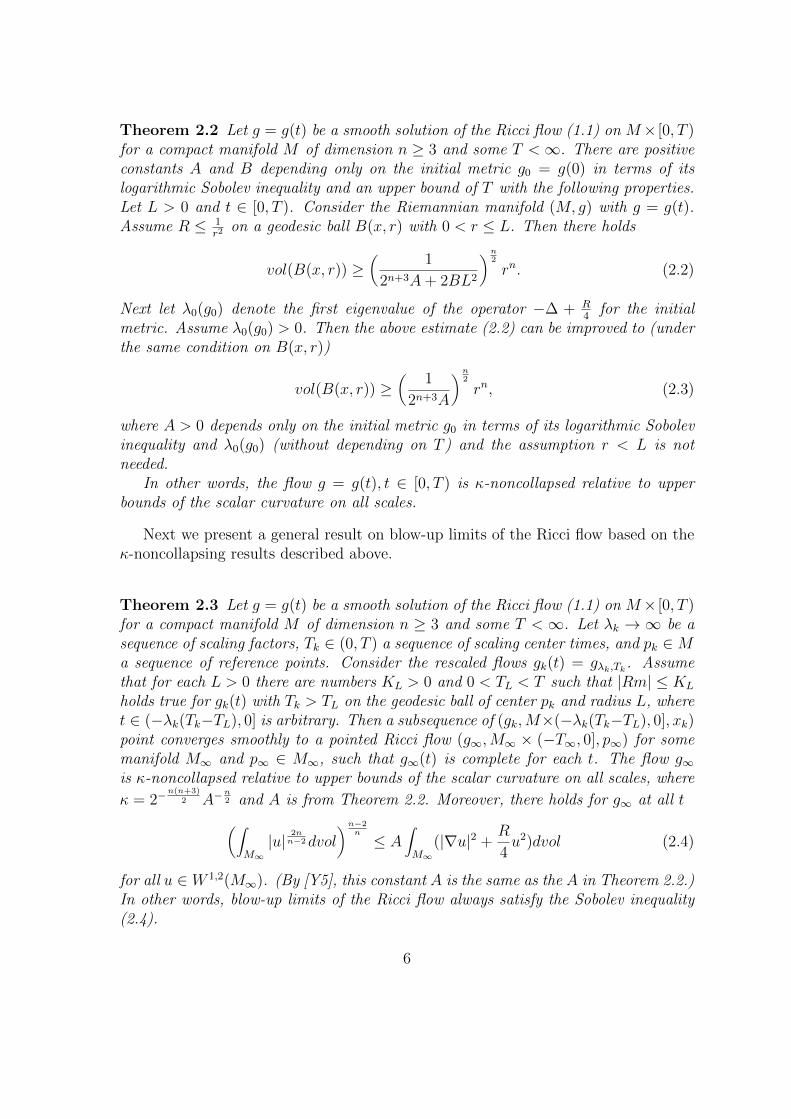
Theorem 2.2 Let g = g(t) be a smooth solution of the Ricci flow (1.1) on M× [0, T )for a compact manifold M of dimension n ≥ 3 and some T <∞. There are positiveconstants A and B depending only on the initial metric g0 = g(0) in terms of itslogarithmic Sobolev inequality and an upper bound of T with the following properties.Let L > 0 and t ∈ [0, T ). Consider the Riemannian manifold (M, g) with g = g(t).Assume R ≤ 1

r2on a geodesic ball B(x, r) with 0 < r ≤ L. Then there holds

vol(B(x, r)) ≥(

1

2n+3A+ 2BL2

)n2

rn. (2.2)

Next let λ0(g0) denote the first eigenvalue of the operator −∆ + R4

for the initialmetric. Assume λ0(g0) > 0. Then the above estimate (2.2) can be improved to (underthe same condition on B(x, r))

vol(B(x, r)) ≥(

1

2n+3A

)n2

rn, (2.3)

where A > 0 depends only on the initial metric g0 in terms of its logarithmic Sobolevinequality and λ0(g0) (without depending on T ) and the assumption r < L is notneeded.

In other words, the flow g = g(t), t ∈ [0, T ) is κ-noncollapsed relative to upperbounds of the scalar curvature on all scales.

Next we present a general result on blow-up limits of the Ricci flow based on theκ-noncollapsing results described above.

Theorem 2.3 Let g = g(t) be a smooth solution of the Ricci flow (1.1) on M× [0, T )for a compact manifold M of dimension n ≥ 3 and some T < ∞. Let λk → ∞ be asequence of scaling factors, Tk ∈ (0, T ) a sequence of scaling center times, and pk ∈Ma sequence of reference points. Consider the rescaled flows gk(t) = gλk,Tk . Assumethat for each L > 0 there are numbers KL > 0 and 0 < TL < T such that |Rm| ≤ KL

holds true for gk(t) with Tk > TL on the geodesic ball of center pk and radius L, wheret ∈ (−λk(Tk−TL), 0] is arbitrary. Then a subsequence of (gk,M×(−λk(Tk−TL), 0], xk)point converges smoothly to a pointed Ricci flow (g∞,M∞ × (−T∞, 0], p∞) for somemanifold M∞ and p∞ ∈ M∞, such that g∞(t) is complete for each t. The flow g∞is κ-noncollapsed relative to upper bounds of the scalar curvature on all scales, where

κ = 2−n(n+3)

2 A−n2 and A is from Theorem 2.2. Moreover, there holds for g∞ at all t(∫

M∞|u|

2nn−2dvol

)n−2n

≤ A∫M∞

(|∇u|2 +R

4u2)dvol (2.4)

for all u ∈ W 1,2(M∞). (By [Y5], this constant A is the same as the A in Theorem 2.2.)In other words, blow-up limits of the Ricci flow always satisfy the Sobolev inequality(2.4).

6

Proof. Note that pointed convergence means convergence on geodesic balls of centerpk and any given radius. By pulling back of metrics, this means convergence ongeodesic balls of center p∞ and any given radius with respect to g∞. By Theorem2.2 the rescaled flow gk satisfies for any given L > 0 and any given time t the volumeestimate

vol(B(p, r)) ≥(

1

2n+3A+ 2BλkL2

)n2

rn, (2.5)

provided that r ≤ L and R ≤ r−2 on B(pk, r) at time t. By the assumption on|Rm| we have for any given time TL ≤ t ≤ Tk the estimate R ≤ c(n)KL on B(pk, L)for a positive constant c(n) depending on n. Hence the volume estimate (2.5) holds

true for p = pk, provided that r ≤ minL,√c(n)KL. By Bishop-Gromov volume

comparison, we then obtain at any t ∈ [−λk(Tk − TL), 0]

vol(B(p, r)) ≥ C(L, n)(

1

2n+3A+ 2BλkL2

)n2

rn (2.6)

for all p ∈ B(pk, L/2), where C(L, n) is a positive constant depending on L and n.By [CGT] (see also [Lemma B.1, Y1]), we obtain a positive constant δ(n, L,A,B)depending on n, L,A and B such that at any t ∈ [−λk(Tk − TL), 0]

i(p) ≥ δ(n, L,A,B) (2.7)

for all p ∈ B(pk, L/2), where i(p) denotes the injectivity radius at p.Now we have for gk upper bounds for |Rm| and positive lower bounds for the

injectivity radius on balls of center pk and radius L/2, over the time interval [−λk(Tk−TL), 0], where L > 0 is arbitrary. Note that these bounds hold uniformly for all gkfor a given L. Moreover, the time interval approaches (−∞, 0] for each L. Now it isquite easy to apply the basic arguments of Gromov-Cheeger-Hamilton compactnesstheorem [H6] to obtain a subsequence of (gk,M×(−λkTk, 0], pk) which point convergessmoothly to a smooth pointed Ricci flow g∞,M∞ × (−∞, 0], p∞).

The stated κ-noncollapsing property of g∞ follows from (2.2) by passing to thelimit. The Sobolev inequality (2.4) follows from the Sobolev inequalities establishedin [Y5].

Two important issues are prompted by this general result. On the one hand,Theorem 2.3 allows one to obtain smooth blow-up limits for the Ricci flow at a blow-up time, provided that one can choose λk, Tk and pk such that the needed curvaturebounds hold. There is a simple situation in which the needed curvature bounds areobviously valid. This is the situation when we choose pk such that the |Rm| of gachieves at (pk, Tk) its maximal value on the domain M × [0, Tk] (one can also usea suitable subinterval of [0, Tk]), and choose λk = |Rm|(pk, Tk)−1. Of course, this

7

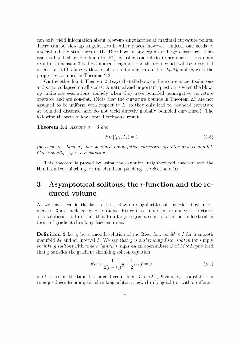
can only yield information about blow-up singularities at maximal curvature points.There can be blow-up singularities in other places, however. Indeed, one needs tounderstand the structures of the Ricc flow in any region of large curvature. Thisissue is handled by Perelman in [P1] by using some delicate arguments. His mainresult in dimension 3 is the canonical neighborhood theorem, which will be presentedin Section 6.10, along with a result on obtaining parameters λk, Tk and pk with theproperties assumed in Theorem 2.3.

On the other hand, Theorem 2.3 says that the blow-up limits are ancient solutionsand κ-noncollapsed on all scales. A natural and important question is when the blow-up limits are κ-solutions, namely when they have bounded nonnegative curvatureoperator and are non-flat. (Note that the curvature bounds in Theorem 2.3 are notassumed to be uniform with respect to L, so they only lead to bounded curvatureat bounded distance, and do not yield directly globally bounded curvature.) Thefollowing theorem follows from Perelman’s results.

Theorem 2.4 Assume n = 3 and

|Rm|(pk, Tk) = 1 (2.8)

for each gk. then g∞ has bounded nonnegative curvature operator and is nonflat.Consequently, g∞ is a κ-solution.

This theorem is proved by using the canonical neighborhood theorem and theHamilton-Ivey pinching, or the Hamilton pinching, see Section 6.10.

3 Asymptotical solitons, the l-function and the re-

duced volume

As we have seen in the last section, blow-up singularities of the Ricci flow in di-mension 3 are modeled by κ-solutions. Hence it is important to analyze structuresof κ-solutions. It turns out that to a large degree κ-solutions can be understood interms of gradient shrinking Ricci solitons.

Definition 3 Let g be a smooth solution of the Ricci flow on M × I for a smoothmanifold M and an interval I. We say that g is a shrinking Ricci soliton (or simplyshrinking soliton) with time origin t0 ≥ sup I on an open subset O of M×I, providedthat g satisfies the gradient shrinking soliton equation

Ric+1

2(t− t0)g +

1

2LXf = 0 (3.1)

in O for a smooth (time-dependent) vector filed X on O. (Obviously, a translation intime produces from a given shrinking soliton a new shrinking soliton with a different

8

time origin.) We say that g is complete, if g(t) is a complete a metric for someeach t ∈ I (equivalently, for some t ∈ I). If X = ∇f for a smooth (time-dependent)function f on O, then g is called a gradient shrinking Ricci soliton (or simply gradientshrinking soliton) and f is called a potential function of f . Note that in this case theequation (3.1) becomes

Ric+1

2(t− t0)g +∇2f = 0. (3.2)

A fixed metric g0 satisfying

Ric+1

2LXg0 = λg0 (3.3)

for a fixed vector field X and a constant λ > 0 will be called a slice shrinking soliton,with “ slice” meaning space slice. (It is also called a shrinking soliton in the literature.Our terminology is for the sake of clarity and convenience.) If X = ∇f , i.e.

Ric+∇2g0 = λg0, (3.4)

then g0 will be called a slice gradient shrinking soliton. It is easy to see that a slicegradient shrinking soliton generates a gradient shrinking soliton g which equals g0

at a time determined by λ and t0. (A similar statement holds true for general sliceshrinking solitons on compact manifolds.)

A shrinking soliton g evolves by the pullback of a family of diffeomorphisms cou-pled with scaling. More precisely, we have

g(t) =t− t0t− t0

φ∗g(t), (3.5)

where t is an arbitary point in I and φ is the solution of the equation

∂φ

∂t= −X (3.6)

with φ(t) = id (id denotes the identity map of M). (Conversely, any g(t) given thisway is a shrinking soliton.) Indeed, we have

∂g

∂t= −2Ric =

1

t− t0g + LXg. (3.7)

Hence∂

∂tφ∗g =

1

t− t0φ∗g. (3.8)

The equation (3.5) follows.

9

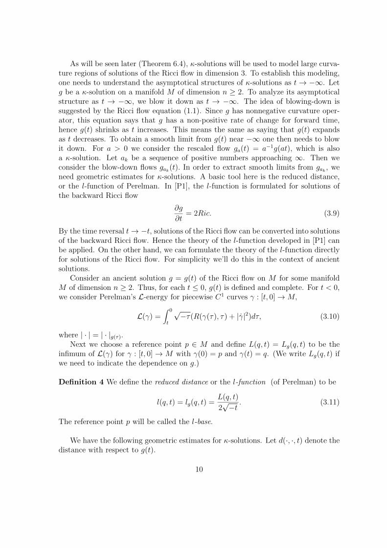
As will be seen later (Theorem 6.4), κ-solutions will be used to model large curva-ture regions of solutions of the Ricci flow in dimension 3. To establish this modeling,one needs to understand the asymptotical structures of κ-solutions as t→ −∞. Letg be a κ-solution on a manifold M of dimension n ≥ 2. To analyze its asymptoticalstructure as t → −∞, we blow it down as t → −∞. The idea of blowing-down issuggested by the Ricci flow equation (1.1). Since g has nonnegative curvature oper-ator, this equation says that g has a non-positive rate of change for forward time,hence g(t) shrinks as t increases. This means the same as saying that g(t) expandsas t decreases. To obtain a smooth limit from g(t) near −∞ one then needs to blowit down. For a > 0 we consider the rescaled flow ga(t) = a−1g(at), which is alsoa κ-solution. Let ak be a sequence of positive numbers approaching ∞. Then weconsider the blow-down flows gak(t). In order to extract smooth limits from gak , weneed geometric estimates for κ-solutions. A basic tool here is the reduced distance,or the l-function of Perelman. In [P1], the l-function is formulated for solutions ofthe backward Ricci flow

∂g

∂t= 2Ric. (3.9)

By the time reversal t→ −t, solutions of the Ricci flow can be converted into solutionsof the backward Ricci flow. Hence the theory of the l-function developed in [P1] canbe applied. On the other hand, we can formulate the theory of the l-function directlyfor solutions of the Ricci flow. For simplicity we’ll do this in the context of ancientsolutions.

Consider an ancient solution g = g(t) of the Ricci flow on M for some manifoldM of dimension n ≥ 2. Thus, for each t ≤ 0, g(t) is defined and complete. For t < 0,we consider Perelman’s L-energy for piecewise C1 curves γ : [t, 0]→M,

L(γ) =∫ 0

t

√−τ(R(γ(τ), τ) + |γ|2)dτ, (3.10)

where | · | = | · |g(τ).Next we choose a reference point p ∈ M and define L(q, t) = Lg(q, t) to be the

infimum of L(γ) for γ : [t, 0] → M with γ(0) = p and γ(t) = q. (We write Lg(q, t) ifwe need to indicate the dependence on g.)

Definition 4 We define the reduced distance or the l-function (of Perelman) to be

l(q, t) = lg(q, t) =L(q, t)

2√−t

. (3.11)

The reference point p will be called the l-base.

We have the following geometric estimates for κ-solutions. Let d(·, ·, t) denote thedistance with respect to g(t).

10

Theorem 3.1 There is a positive constant C depending only on the dimension nsuch that

R ≤ Cl

|t|(3.12)

everywhere on M × (−∞, 0],

|∇l|2 ≤ Cl

|t|(3.13)

almost everywhere in M for each t ∈ (−∞, 0],

|√l(q1, τ)−

√l(q2, t)| ≤

√C

4|t|d(q1, q2, t) (3.14)

for all t ∈ (−∞, 0] and all q1, q2 ∈M , and

|lt| ≤Cl

|t|(3.15)

almost everywhere in (−∞, 0] for each q ∈ M . Moreover, we have the followingHarnack inequality

(t1t2

)C ≤ l(q, t2)

l(q, t1)≤ (

t2t1

)C (3.16)

for all q ∈M and t1, t2 ∈ (−∞, 0] with |t2| > |t1|.

Proof. This follows from [Theorem 2.18, Y2], which is based on Perelman’s estimatesin [P1] and the analytic properties of the l-function established in [Y2].

Lemma 3.2 For each t ∈ (−∞, 0], there is a minimum point p(t) of l(·, t). Moreover,there holds l(p(t), t) ≤ n/2.

Proof. The upper bound follows from Section 7.1 of [P1], see also [Lemma 3.1, Y2].The existence of pt follows from [Lemma 2.3, Y2].

Based on the above geometric estimates we can now extract smooth blow-downlimits from a κ solution g(t). The following theorem is formulated in [Y3] as part of[Proposition 11.2, P1].

Theorem 3.3 Let g = g(t) be a κ-solution on a manifold M of dimension n ≥ 2 asbefore. Let tk → −∞ be given. For each tk, let p(tk) be a minimum point of l(·, t).Then the pointed flows (g|tk|,M×(0,∞), p(tk)) subconverge smoothly to pointed smoothsolutions (g∞,M∞× (−∞, 0), p∞) of the Ricci flow, which will be called asymptoticallimits of g. These limits are κ-noncollapsed on all scales.

11

Proof. We reproduce the proof given in [Y3]. The various quantities associated withg|tk| will be indicated by the subscript k or g|tk|, e.g. lk = lg|tk| and dk = dg|gk| . ByLemma 3.2 and the scaling invariance of the l-function we have

lk(p(tk),−1) ≤ n

2. (3.17)

By this estimate and [Lemma 3.2, Y2] we infer

lk(q,−1) ≤ C2d2k(x(τk), q,−1) + n (3.18)

for all q ∈ M , where C2 is a positive constant depending only on the dimension n.Then it follows from the Harnack inequality (3.16) that

lk(q, t) ≤ |t|±C(C2(d2k(p(tk), q,−1) + n), (3.19)

where ± = + if |t| ≥ 1, ± = − if |t| < 1, and C is a positive constant dependingonly on n. Consequently, we obtain from (3.12) and the nonnegativity of curvatureoperator the estimate

|Rm|k(q, t) ≤ C|t|−1±C(d2k(p(tk), q,−1) + 1). (3.20)

By the κ-noncollapsing property of gk we then obtain the desired pointed smoothconvergence to pointed solutions (g∞,M∞ × (0,∞), x∞) of the Ricci flow as in theproof of Theorem 2.3. The κ-noncollapsing property of g∞ follows from the κ-noncollapsing property of gk and the smooth convergence.

The next stage of the process of understanding κ-solutions is to identify asymp-totical limits to be gradient shrinking solitons. A crucial tool for this purpose is thereduced volume of Perelman. For convenience we again formulate it for the Ricci flowrather than the backward Ricci flow as in [P1], and restrict the discussion to ancientsolutions.

Definition 5 Let g be an ancient solution of the Ricci flow on a manifold M ofdimension n ≥ 2. Choose a point p as the l-base. We define the reduced volume (ofPerelman) to be

V (t) = Vg(t) =∫M|t|−

n2 e−l(q,t)dvolg(t). (3.21)

It is easy to see that V is invariant under the rescaling g → ga. The key propertiesof the reduced volume are its monotonicity, upper bounds, and the associated rigidi-ties. The following results were obtained in [Y2] (in the formulation of the backwardRicci flow), which include Perelman’s results on the reduced volume in [P1] as specialcases. The basis for these results is Perelman’s differential inequality [P1]

d

dt(|t|−

n2 e−l(v,t)J(t)(v)) ≥ 0 (3.22)

12

and the analytic properties of the l-function established in [Y2]. Here v is a tangentvector at p which lies in the injectivity domain of the L-exponential map (the expo-nential map associated with the L-geodesics), l(v, t) = l(γv(t), t) with γv denoting theL-geodesic determined by the initial tangent vector v, and J(t) denotes the Jacobianof the L-exponential map.

Theorem 3.4 If the Ricci curvature is bounded from below on [T, 0] for each T < 0,then V (t) is a nondecreasing function.

Theorem 3.5 Assume that the Ricci curvature is nonnegative for s ∈ [t, 0]. ThenV (t) < (4π)

n2 unless (M, g(0)) is isometric to Rn and g(s) = g(0) for all s ∈ [t, 0], in

which case V (t) = (4π)n2 .

The next theorem is formulated in [Y3] as the remaining part of [Proposition 11.2,P1].

Theorem 3.6 Let (g∞,M∞ × (0,∞), p∞) be an asymptotical limit of a κ-solutiong. Then g∞ is a nonflat gradient shrinking soliton with time origin 0. Moreover,the limit l-function l∞ is a potential function. Henceforth asymptotical limits will becalled “asymptotical solitons”.

Here the limit l-function l∞ refers to the limit of the sequence of l-functions lg|tk|for the associated sequence of rescaled flows g|tk| (as in Theorem 3.3). The applicationof the reduced volume in the proof of this theorem as presented in [Y3] is in terms ofthe asymptotical reduced volume V∞ of g∞, which is the limit of the reduced volumeof g|tk|. By the monotonicity of the reduced volume (Theorem 3.4) and a delicate

convergence argument one deduces that V∞(t) is independent of time t. On the otherhand, one has

V∞(t2)− V∞(t1) = −∫ t2

t1

∫M∞

(∂l∞∂t

+R∞ +n

2t)e−l∞ |t|−

n2 dqdt (3.23)

for t1 < t2, which follows from another delicate argument about absolute convergenceof improper integrals. (The subscript ∞ for various quantities refers to g∞.) Thuswe have ∫ t2

t1

∫M∞

(∂l∞∂t

+R∞ +n

2t)e−l∞|t|−

n2 dqddt = 0. (3.24)

Besides this identity, another important tool employed in the proof of Theorem3.6 is the following lemma.

Lemma 3.7 The equation

∂l∞∂t

+R∞2− |∇l∞|

2

2+l∞2t

= 0 (3.25)

13

holds true almost everywhere on M∞ × (0,∞). The inequality

∆l∞ −|∇l∞|2

2+R∞2

+l∞ − n

2τ≤ 0 (3.26)

holds true for each t < 0 in the weak sense, i.e.∫M∞−∇l∞ · ∇φ+

1

2(−|∇l∞|2 +R∞ −

l∞ − nt

)φdq ≤ 0 (3.27)

for all nonnegative Lipschitz functions φ with compact support. Finally, the inequality

∂l∞∂t

+ ∆l∞ − |∇l∞|2 +R∞ +n

2t≤ 0 (3.28)

holds true on M∞ × (0,∞) when ∆ is interpreted in the weak sense, i.e.

Qt1,t2(φ) ≤ 0 (3.29)

for arbitray t1 < t2 < 0 and nonnegative Lipschitz functions φ on M∞ × [t1, t2] withcompact support, where

Qt1,t2(φ) =∫ t2

t1

∫M∞−∇l∞ · ∇φ+ (

∂l∞∂t− |∇l∞|2 +R∞ +

n

2t)φdqdt. (3.30)

This lemma is derived in two stages. First a similar lemma is derived for gk,based on Perelman’s differential inequalities in [P1] and the analytic properties ofthe l-function established in [Y2]. Then Lemma 3.7 is derived via a convergenceargument. Here, a lemma about strong convergence of Sobolev functions establishedin [Y3] is needed. (see [Y3] for details.) (In [Y3], this lemma is formulated in termsof the variable τ = −t.)

Now we have all the ingredients needed to finish the proof of Theorem 3.6. Notethat the identity (3.24) means Qt1,t2(|t|−

n2 e−l∞) = 0. Combining this with Lemma

3.7 one infers that the inequalities in Lemma 3.7 become equalities, and the functionl∞ is smooth (as a consequence of parabolic regularity). Then one appeals to thecharacterization of gradient shrinking solitons in terms of these differential equalities(see [P1] and [Y2]) to conclude that g∞ is a gradient shrinking soliton with potentialfunctional l∞. The nonflat property of l∞ is derived by using the strict upper boundfor the reduced volume of gk provided by Theorem 3.5. We refer to [Y3] for details.

4 Classification of 2-dimensional κ-solutions

As shown in [P1][P2] and will be discussed in Sections 5 and 6, the following resultplays an important role in analyzing structures of 3-dimensional κ-solutions and blow-up singularities of the Ricci flow in dimension 3.

14

Theorem 4.1 In dimension 2 round spheres are the only orientable κ-solutions.

This theorem is precisely [Corrolary 11.3, P1]. Its proof given in [P1] is incom-plete, since it leaves out the case of noncompact 2-dimensional κ-solutions. Here wereproduce the first complete proof of this result which is presented in the present au-thor’s paper [Y4]. (This paper has been available at the author’s website and throughthe website of B. Kleiner and J. Lott and the references in their notes on Perelman’spapers on the Ricci flow [KL] since early 2004.)

There is a gradient shrinking Ricci soliton g∗ with time origin 0 on S2 which is givenby g∗(t) = −2tgS2 . Its potential functions are the constant functions. We can shiftits time origin, rescale it by a constant factor, and pull it back by a diffeomorphism.The shrinking Ricci solitons obtained this way will be called round sphere solitons.By a round sphere metric on a manifold M diffeomorphic to S2 we mean λF ∗gS2 ,where λ is a positive number and F is a smooth diffeomorphism from M onto S2.

Lemma 4.2 Let M be diffeomorphic to S2 and g a shrinking Ricci soliton on M .Then g is a round sphere soliton.

Proof. This follows from [Theorem 10.1, H1]. For a different proof based on [BSY],we refer to [Y4].

Lemma 4.3 Let g be a smooth solution of the Ricci flow on M × (a, b) for a 2-dimensional manifold M and some time interval (a, b), such that for each t ∈ (a, b),the metric g(t) is complete and has nonnegative scalar curvature. Moreover, assume∂R∂t≥ 0. Let t0 ∈ (a, b). Assume that g(t0) is κ-noncollapsed on the scale ρ for some

κ > 0 and ρ > 0. Then g(t0) has bounded scalar curvature.

Proof. The proof is along the lines of arguments in several places in [P1]. Ourargument for point picking is more direct. We’ll add the notation t explicitly tovarious quantities to indicate the metric g(t) at time t, e.g. B(p, r, t) is the geodesicball of center p and radius r with respect to the metric g(t). Assume that g(t0)has unbounded scalar curvature. Choose a sequence of points pk ∈ M such thatR(pk, t0) > 0 for each k and R(pk, t0) → ∞. Choose qk ∈ B(pk, 1, t0) such that thefunction d(·, ∂B(pk, 1, t0), t0)2R(·, t0) on B(pk, 1, t0) achieves its maximum at qk. Weset rk = d(qk, ∂B(pk, 1, t0), t0)/2. For q ∈ B(qk, rk, t0) we have d(q, ∂B(pk, 1, t0), t0) ≥rk and hence the maximum property of qk implies

r2kR(q, t0) ≤ d(q, ∂B(pk, 1, t0), t0)2R(q, t0) ≤ 4r2

kR(qk, t0). (4.1)

It follows that

R(q, t0) ≤ 4R(qk, t0) (4.2)

15

onB(qk, rk, t0). By the maximum property of qk we also infer r2kR(qk, t0) ≥ R(pk, t0)/4,

so rk > 0 for each k and r2kR(qk, t0) → ∞. On the other hand, it is obvious that

qk → ∞. Now we consider the rescaled flows gk(t) = R(qk, t0)g(t0 + R(qk, t0)t). Set

ρk = rk√R(qk, t0). There holds R(qk, 0) = 1 and R(·, 0) ≤ 4 on B(qk, ρk, 0) for gk. By

the property ∂R∂t≥ 0 we can control the curvature for t ≤ 0 as well. Combining this

with the κ-noncollapsing condition we then obtain from (M, gk, qk) a smooth limit(g∞,M∞, p∞). By Splitting Lemma in [Appendix, Y4] or [Appendix G, KL] this limitsplits off a line, i.e. is the isometric product of a lower dimensional manifold withR. (We only need the splitting at t = 0, although it holds for the flow.) Since M∞is 2-dimensional, it follows that g∞ is flat. But the scalar curvature of R(qk, t0)g(t0)at qk is 1, hence the scalar curvature of g∞(0) at q∞ is also 1. This is a contradiction.

Note that by Lemma 2.1 and smooth convergence asymptotical solitons have non-decreasing scalar curvature, i.e. satisfy ∂R

∂t≥ 0.

Lemma 4.4 Let g be a 2-dimensional asymptotical soliton, or, more generally, acomplete nonflat κ-noncollapsed gradient shrinking soliton with non-negative and non-decreasing scalar curvature. Then it is a round sphere soliton.

Proof. By time translations we may assume that 0 is the time origin of g. Hence gsatisfies the soliton equation

Ric+1

2tg +∇2f = 0. (4.3)

By Lemma 4.3, g has bounded scalar curvature for each t < 0. We also observe thatR is everywhere positive. Indeed, if R is zero at some point p and some time t, thenthe strong maximum principle applied to the evolution equation of R

∂R

∂t= ∆R +R2 (4.4)

implies that R is everywhere zero, which contradicts the nonflatness of g.We claim that M is compact. To prove the claim, fix a point p0 ∈ M . Following

[(1.2), P2] we have, as a consequence of (4.3) the following equation

dR = 2Ric(∇f, ·) = Rg(∇f, ·) = Rdf. (4.5)

Let θ(q, t, γ) denote the (smaller) angle between∇f(q, t) and γ′(l), where l = d(p0, q, t)and γ is a unit speed shortest geodesic with respect to g(t) such that γ(0) = p0 andγ(l) = q. This angle is defined to be 2π if ∇f(q, t) = 0. By the arguments in theproof of [Lemma 1.2, P2] in [P2], there is a positive number A0 such that

θ(q,−1, γ) ≤ π

4(4.6)

16

whenever d(p0, q,−1) ≥ A0.Let γ be a shortest geodesic from p0 to a point q with d(p0, q,−1) > A0. We have

by (6.8) and (4.6)

d

dtR(γ(t),−1) = ∇R · γ′(t) = R∇f · γ′(t) > 0, (4.7)

as long as t ≥ A. Thus R(γ(t),−1) increases along the portion of γ which lies outsideof the geodesic ball B(p0, A0,−1). Consequently, we obtain the following estimate

R(q,−1) ≥ αA0 (4.8)

for all q ∈ M , where αA0 = minR(q,−1) : q ∈ B(p0, A0,−1). Since R > 0everywhere, αA is positive. By Bonnet theorem, M must be compact.

Now we apply Gauss-Bonnet theorem to infer that M is diffeomorphic to S2. Thenwe apply Lemma 4.2 to conclude that (M, g) is a round sphere soliton.

Remark This result extends to other classes of shrinking solitons, see [Y4].

Proof of Theorem 4.1Let (M, g∗) be an orientable 2-dimensional κ-solution. Consider an arbitary

asymptotic soliton (M∞, g∞, q∞) of g∗ given by Theorem 3.3 and Theorem 3.6. ByLemma 4.4, (M∞, g∞) is a round sphere soliton. Consequently, M is diffeomorphicto S2. Moreover, modulo smooth diffeomorphisms of M , the metrics 1

|t|g∗(t) converge

smoothly on M to metrics of positive constant scalar curvature as t→ −∞.We set g(τ) = λ(t)g∗(t) with λ(t) = exp(

∫ t−1 r

∗) and τ =∫ t−1 λ, where r∗(t) denotes

the average scalar curvature of g∗(t). Then g = g(τ) satisfies the volume-normalizedRicci flow

∂g

∂τ= (r −R)g (4.9)

with r denoting the average scalar curvature of g. There holds τ ∈ (Λ1,Λ2], whereΛ1 = limt→−∞ τ(t) and Λ2 = τ(0), Then, modulo smooth diffeomorphisms of M , g(τ)converges to metrics of positive constant scalar curvature as τ → Λ1. Following [H1],let f be the solution of ∆f = R− r with mean value zero, and set H = ∇2f − 1

2∆fg

(Hij is the Mij in [H1]). By [(9.1), H1] we have

∂|H|2

∂τ= ∆|H|2 − 2|∇H|2 − 2R|H|2. (4.10)

Hence the maximum principle implies that max |H|2 is nonincreasing. Since g con-verges modulo smooth diffeomorphisms of M to metrics of positive constant scalarcurvature as τ → Λ1, we have H → 0 as τ → Λ1, whence H ≡ 0. Now, pulling back

17

g by a family of diffeomorphisms φ(t) generated by ∇f with φ(−1) = id, we obtaing which satisfies

∂g

∂τ= 2H = 0. (4.11)

Thus g is independent of time. Since its scalar curvature approaches a positive con-stant as τ → Λ1, we infer that g has positive constant scalar curvature. It followsthat g and hence g∗ has positive constant scalar curvature. We conclude that g∗ isa round sphere κ-solution. Note that we have f ≡ 0 because g has constant scalarcurvature. Consequently, g = g. We deduce that g∗(t) = λ(t)g for positive scalarsλ(t). This immediately yields g∗(t) = (1 − 2

nR0t)g

∗(0), where R0 denotes the scalarcurvature of g∗(0).

5 Classification of 3-dimensional κ-solutions and

Perelman’s compactness theorem

In [P2], Perelman obtained the classification of 3-dimensional κ-solutions based ona classification of 3-dimensional gradient shrinking solitons. One ingredient in thisclassifications is the classification of 2-dimensional κ-solutions and gradient shrink-ing solitons presented in the last section. Perelman’s classification of 3-dimensionalgradient shrinking solitons in [P2] is as follows.

Theorem 5.1 Let g be a complete, κ-noncollapsed gradient shrinking soliton withbounded nonnegative sectional curavture on a 3-dimensional manifold M . Then theuniversal cover of (M, g) is isometric to R3, S3 or S2×R, where S2 is equipped witha constant multiple of the round sphere metric of sectional curvature 1.

The key ingredient for establishing this theorem is Lemma 1.2 in [P2] which westate below as a theorem.

Theorem 5.2 There is no 3-dimensional complete, noncompact and nonflat gradientshrinking soliton which is κ-noncollapsed and has bounded positive sectional curvature.

One argument in the proof of this theorem in [P2] uses Theorem 4.1. (The aboveproof of Lemma 4.4 offers some aspect of this argument.) Another argument is interms of the level surfaces of the potential function of the soliton. We refer to [P2]for details.

Proof of Theorem 5.1 By Theorem 5.2, one is left to handle a compact universalcover or a noncompact universal cover whose sectional curvature is not strictly posi-tive everywhere. In the former case, the Ricci curvature must be positive. Otherwise,

18

Hamilton’s strong maximum principle [H2] implies a splitting, i.e. the universal cover(M, g) is the isometric product of a 1-dimensional factor and a 2-dimensional factor.This is impossible because the only possible 1-dimensional factor is S1, which is ex-cluded by the simple connectedness. Then the conclusion follows from Hamilton’stheorem on the Ricci flow on compact 3-manifolds of positive Ricci curvature in [H1].In the latter case, by Hamilton’s strong maximum principle the universal cover (M, g)splits off a line. If the 2-dimensional factor is flat, then it must be R2. It follows that(M, g) is isometric to R3. If the 2-dimensional factor is nonflat, then it is a roundsphere soliton by Lemma 4.4 and Lemma 2.1. Thus (M, g) is isometric to S2×R.

Recently, Perelman’s classification was extended by L. Ni-N. Wallach [NiW] andA. Naber [Na] to 3-dimensional complete shrinking solitons of bounded nonnega-tive Ricci curvature by using different methods. Ni and Wallach used an evolutionequation of curvature quantities associated with the Ricci flow and an integrationargument, while Naber used the l-function, the reduced volume and the potentialfunction. (Ni-Wallach only treated gradient shrinking solitons. But they allow un-bounded curvature which satisfies a certain growth condition.) We state their resultin the following theorem.

Theorem 5.3 Let g be a complete shrinking soliton of bounded nonnegative Riccicurvature on a 3-dimensional manifold M . Then the universal cover of (M, g) isisometric to R3, S3 or S2 ×R.

Based on the 3-dimensional classification of gradient shrinking solitons and theresults on asymptotical solitons (namely Theorem 3.3 and Theorem 3.6) Perelmanobtained the following classification of 3-dimensional κ-solutions.

Theorem 5.4 Let (M, g) be a 3-dimensional κ-solution. Then it falls into one of thefollowing three mutually exclusive cases:1. It has an asymptotical soliton which is isometric to a metric quotient of the round3-dimensional sphere. In this case, (M, g) is isometric to a metric quotient of theround 3-dimensional sphere. (This case is the same as the case that (M, g) has acompact aymptotical soliton.)2. It has an asymptotical soliton which is isometric to the nontrivial Z2 quotient ofS2 ×R. In this case, a nontrivial isometric Z2 cover of (M, g) has an asymptoticalsoliton which is isometric to the round cylinder S2×R. (This case is the same as thecase that (M, g) has an asymptotical soliton which contains the one-sided projectiveplane.)3. It has an asymptotical soliton which is isometric to the round cylinder S2×R. Inthis case, M can be noncompact or compact.Finally, if (M, g) is compact, but has a noncompact asymptotical soliton, then M isdiffeomorphic to S3 or RP3.

19

Proof. The three types of asymptotical solitons follow from Theorem 5.1. In Case 1,M is obviously compact. By Theorem 3.3 and Theorem 3.6, there is a sequence oftimes tk →∞, such that |tk|−1g(tk) approaches a metric of constant positive sectionalcurvature. By Hamilton’s results in [H1] the Ricci curvature is positive for all t ≤ tk.Moreover, the pinching of the Ricci curvature improves along g in the forward timedirection. Hence the Ricci curvature is no less pinched at t ≥ tk than at tk. For afixed t we let k → ∞ and conclude that the Ricci curvature is zero pinched at t. Itfollows that (M, g) is isometric to a metric quotient of the round 3-sphere.

The last statement does not seem to be in Perelman’s papers. It is [Lemma 59.3,KL]. We refer to [KL] for its proof.

Examples in Case 3 include the round cylinder itself and Bryant soliton whichis a steady Ricci soliton on R3. In [1.4, P2] Perelman presented a construction ofcompact examples. More detailed classifications of κ-solutions are certainly desirable,but Theorem 5.4 is sufficient for the purposes in [P1], [P2] and [P3].

Next we would like to present Perelman’s compactness theorem for the space of3-dimensional noncompact κ-solutions. This result is very useful for deriving geo-metric estimates for κ-solutions themselves and general solutions of the Ricci flow indimension 3. Before stating the compactness theorem, we state Perelman’s result onthe asymptotical volume ratio, which is a tool for proving the compactness theorem.Let (M, g) be an n-dimensional noncompact, complete Riemannian manifold of non-negative Ricci curvature and p ∈ M . By Bishop-Gromov volume comparison, theratio function vol(B(p, r))/rn is nonincreasing in r. Let V = V(M, g) denote its limitas t→∞. It is independent of p and called the asymptotical volume ratio of (M, g).

Theorem 5.5 Let (M, g) be a κ-solution of dimension n ≥ 3. Then V(M, g(t)) = 0for each t.

The proof of this theorem given in [P1] is by induction on the dimension. Ituses the concept of asymptotical scalar curvature ratio, rescaling limits and splittingarguments. We refer to [P1], [KL] and [MT] for details.

Theorem 5.6 The space of 3-dimensional noncompact κ-solutions is compact moduloscaling. More precisely, let (Mk, gk) be a sequence of 3-dimensional noncompact κ-solutions, and let pk be a point of Mk for each k. Let λk denote the scalar curvatureof gk(0) at pk. (By the strong maximum principle, λk > 0.) Then a subsequenceof the pointed κ-solutions (Mk, gk, pk) with gk = λkgk point converges smoothly to aκ-solution (M∞, g∞, p∞).

Proof. It suffices to consider orientable κ-solutions, because we can pass to the ori-entable double cover for an unorientable κ-solution. Note that R(pk, 0) = 1 for gk. Inthe first part of the proof given in [P1] one shows that for each given (finite) radiusL the scalar curvature R is bounded on B(pk, L, 0). This is done by a contradictionargument involving Theorem 5.5. We refer to [P1], [KL] and [MT] for details.

20

Given the result of bounded scalar curvature at bounded distances, we also havebounded curvature operator at bounded distance because the curvature operatoris nonnegative. Hence we can argue as in Theorem 2.3 to obtain a pointed limit(M∞, g∞, p∞) from a subsequence of (Mk, gk, pk). This limit is κ-noncollapsed on allscales and has nonnegative curvature operator. Moreover, it satisfies ∂R

∂t≥ 0. To

obtain the desired κ-solution property, it remains to show that it has bounded scalarcurvature at t = 0. Assume the contrary. Then we can find a sequence of pointspk in M∞ going to ∞, such that R(pk, 0) → ∞. Then we choose points qk as inthe proof of Lemma 4.3. Now we set λk = R(qk, 0) and consider the rescaled flowsg∞,k(t) = λkg∞(λ−1

k t). Then we have R(qk, 0) = 1 and R(·, 0) ≤ 4 on B(qk, ρk, 0) forgk, where ρk →∞. By the property ∂R

∂t≥ 0 we can control R for t < 0 as well. Com-

bining this with the κ-noncollapsing property we can then obtain a smooth pointedlimit flow (M∞

∞ , g∞,∞), which is obviously a κ-solution. By the splitting argumentalluded to in the proof of Lemma 4.3, this limits splits off a line. By Theorem 4.1,the 2-dimensional factor must be a round sphere. It follows that this limit is theround cylinder S2 ×R. Consequently, qk is contained in a neck-like region Zk whichapproaches the round cylinder after the dilation by the factor λk, which approaches∞. (So Zk is getting thinner and thinner, while getting longer and longer relative tothe cross size.) This is impossible in a noncompact, complete manifold of nonnegativesectional curvature, see e.g. [46.1, KL]. (A result in [S] is used here.)

6 Achieving bounded curvature and the canonical

neighborhood theorem

As a preparation for the main content of this seciton, we first present the conceptof Hamilton-Ivey pinching and Hamilton pinching, which is a key property of theRicci flow in dimension 3. The Hamilton pinching condition is an improvement ofthe Hamilton-Ivey pinching condition and contains additional useful information forlarge time. For bounded time, it suffices to use the Hamilton-Ivey pinching condition.

Defintion 6 Let M be a manifold of dimension 3.A. Let g be a smooth metric M . Let ν(p) denote the smallest eigenvalue of thecurvature operator of g at p. We say that g satisfies the Hamilton-Ivey pinchingcondition, if R(p) ≥ −1, and

f−1(R) ≥ −ν(p), (6.1)

for all p ∈M , where f denotes the function x lnx− x defined for x ≥ 1.B. Let g be a smooth metric on M and t a nonnegative number. We say that gsatisfies the Hamilton pinching condition at time t, if there holds at each p

R(p) ≥ − 3

1 + t(6.2)

21

and one of the following two inequalities holds true1) ν(p) ≥ 0,2)

R(p) ≥ |ν(p)| (ln |ν(p)|+ ln(1 + t)− 3) . (6.3)

The first theorem below is due to Hamilton [H5] and Ivey [I]. The second is dueto Hamilton [H5].

Theorem 6.1 The Ricci flow preserves the Hamilton-Ivey pinching condition onclosed 3-manifolds. It also preserves the Hamilton-Ivey pinching condition amongcomplete metrics with bounded sectional curvatures on noncompact 3-manifolds.

Theorem 6.2 The Ricci flow preserves the Hamilton pinching condition on closed3-manifolds. More precisely, let g0 be a metric on a closed manifold M satisfying theHamilton time-t0 pinching condition. Let g = g(t) be a smooth solution of the Ricciflow on M× [t0, T ) for some T > t0 with g(0) = g0. Then g = g(t), t ∈ [t0, T ) satisfiesthe Hamilton pinching condition.

The Ricci flow also preserves the Hamilton pinching condition among completemetrics with bounded sectional curvatures on noncompact 3-manifolds.

These two results are proved by employing the maximum principle. They dependin a strong way on the special structures of the curvature operator in dimension 3.The present author is not aware of any counterexample in higher dimensions. So onemay wonder to what extent they can be extended to higher dimensions. The followingsimple lemma demonstrates why Hamilton-Ivey pinching and Hamilton pinching areso useful.

Lemma 6.3 For each k let gk be a smooth metric on a 3-manifold Mk satisfyingthe Hamilton-Ivey pinching condition. Let λk → ∞ and pk ∈ Mk. Assume that(λkgk,Mk, pk) point converge smoothly to a pointed Riemannian manifold (M∞, g∞, p∞).Then g has nonnegative curvature operator. We have the same conclusion if theHamilton-Ivey pinching is replaced by the Hamilton pinching at a fixed t.

Proof. We treat the case of the Hamilton-Ivey pinching. The case of the Hamiltonpinching is similar. Note that the pinching condition (6.1) means

R ≥ |ν|(ln |ν| − 1) (6.4)

when ν ≤ −1. So the ratio of R over |ν| for gk goes to ∞ when ν is negative and|ν| goes to ∞ along gk and some points. After scaling gk by the factor λk, and hencescaling its curvature quantities by λ−1

k , R converges and hence is bounded by the

22

assumption. Consequently, the rescaled |ν| must go to zero because it is scaled bythe same factor as R. On the other hand, if ν is negative but does not go to ∞,then the rescaled ν must go to zero because λk → ∞. In the remaining case, ν isnonnegative, then the limit of the rescaled ν is obviously nonnegative. These threecases may happen along different subsequences, and this argument is applied to eachsituation.

Next we present Perelman’s theorem on canonical neighborhoods of solutions ofthe Ricci flow in dimension 3. It is based on two results, one is Perelman’s theoremof modeling large curvature regions of the Ricci flow by κ-solutions. The other isPerelman’s theorem on the canonical neighborhood property of κ-solutions. Theformer is [Theorem 12.1, P1], with a slight modification given in [Theorem 52.3, KL],the latter is a result presented in Section 1.5 of [P2]. We state them below in thisorder. (In the statements of Theorem 6.4 we make a simplification by dropping theT which appears in [Theorem 12.1, P1] and [Theorem 52.3, KL].)

Theorem 6.4 Given ε > 0, κ > 0 and ρ > 0, one can find r0 > 0 with the followingproperty. If g = g(t), 0 ≤ t ≤ t0 with t0 ≥ 1 is a smooth solution of the Ricci flowon a closed 3-manifold M , which satisfies the Hamilton-Ivey pinching condition (orthe Hamilton pinching condition) and is κ-noncollapsed on scales < ρ, then for anypoint p0 with Q = R(p0, t0) ≥ r−2

0 , the solution in (p, t) : d2(p, p0, t0) < (εQ)−1, t0 −(εQ)−1 ≤ t ≤ t0, is, after scaling by the factor Q, ε-close to the corresponding subsetof some κ-solution.

This theorem is proved by an intricate contradiction argument involving delicatelimiting arguments. Here two metrics are said to be ε-close if the Cε-norm (mea-sured with respect to one of the two metrics) of the difference of the two metricsdoes not exceed ε. (For two metrics on two different manifolds this involves pullingback of metrics.) Note that e.g. C3.14 means the Holder space C3,0.14. Perelman’sarguments for proving this theorem extend to noncompact, complete manifolds withan assumption on curvature bounds, see e.g. [KL]. It is for simplicity of statementsthat this theorem is only formulated for closed manifolds. For convenience, we statethe implication of Theorem 6.4 for the case 0 < t0 < 1 as a theorem.

Theorem 6.5 Given ε > 0, κ > 0 and ρ > 0, one can find r0 > 0 with thefollowing property. If g = g(t), 0 ≤ t ≤ t0 with 0 < t0 ≤ 1 is a smooth solu-tion of the Ricci flow on a closed 3-manifold M , which satisfies the Hamilton-Iveypinching condition (or the Hamilton pinching condition) and is κ-noncollapsed onscales < ρ

√t0, then for any point p0 with Q = R(p0, t0) ≥ t−1

0 r−20 , the solution in

(p, t) : d2(p, p0, t0) < (εQ)−1, t0 − (εQ)−1 ≤ t ≤ t0, is, after scaling by the factor Q,ε-close to the corresponding subset of some κ-solution.

Proof. Consider the rescaled solution g = t−10 g(t0t). Applying Theorem 6.4 and

scaling the result back to g.

23

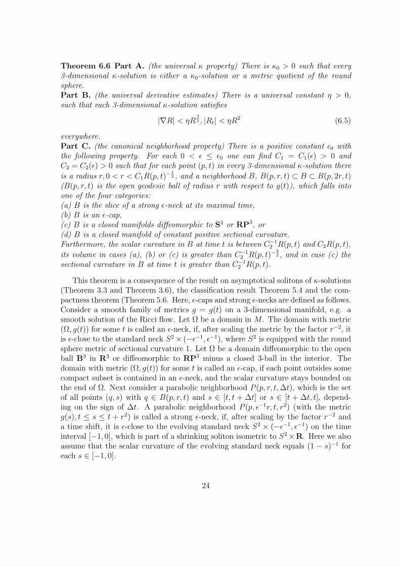
Theorem 6.6 Part A. (the universal κ property) There is κ0 > 0 such that every3-dimensional κ-solution is either a κ0-solution or a metric quotient of the roundsphere.Part B. (the universal derivative estimates) There is a universal constant η > 0,such that each 3-dimensional κ-solution satisfies

|∇R| < ηR32 , |Rt| < ηR2 (6.5)

everywhere.Part C. (the canonical neighborhood property) There is a positive constant ε0 withthe following property. For each 0 < ε ≤ ε0 one can find C1 = C1(ε) > 0 andC2 = C2(ε) > 0 such that for each point (p, t) in every 3-dimensional κ-solution there

is a radius r, 0 < r < C1R(p, t)−12 , and a neighborhood B, B(p, r, t) ⊂ B ⊂ B(p, 2r, t)

(B(p, r, t) is the open geodesic ball of radius r with respect to g(t)), which falls intoone of the four categories:(a) B is the slice of a strong ε-neck at its maximal time,(b) B is an ε-cap,(c) B is a closed manifolds diffeomorphic to S3 or RP3, or(d) B is a closed manifold of constant positive sectional curvature.Furthermore, the scalar curvature in B at time t is between C−1

2 R(p, t) and C2R(p, t),

its volume in cases (a), (b) or (c) is greater than C−12 R(p, t)−

32 , and in case (c) the

sectional curvature in B at time t is greater than C−12 R(p, t).

This theorem is a consequence of the result on asymptotical solitons of κ-solutions(Theorem 3.3 and Theorem 3.6), the classification result Theorem 5.4 and the com-pactness theorem (Theorem 5.6. Here, ε-caps and strong ε-necks are defined as follows.Consider a smooth family of metrics g = g(t) on a 3-dimensional manifold, e.g. asmooth solution of the Ricci flow. Let Ω be a domain in M . The domain with metric(Ω, g(t)) for some t is called an ε-neck, if, after scaling the metric by the factor r−2, itis ε-close to the standard neck S2× (−ε−1, ε−1), where S2 is equipped with the roundsphere metric of sectional curvature 1. Let Ω be a domain diffeomorphic to the openball B3 in R3 or diffeomorphic to RP3 minus a closed 3-ball in the interior. Thedomain with metric (Ω, g(t)) for some t is called an ε-cap, if each point outsides somecompact subset is contained in an ε-neck, and the scalar curvature stays bounded onthe end of Ω. Next consider a parabolic neighborhood P (p, r, t,∆t), which is the setof all points (q, s) with q ∈ B(p, r, t) and s ∈ [t, t + ∆t] or s ∈ [t + ∆t, t], depend-ing on the sign of ∆t. A parabolic neighborhood P (p, ε−1r, t, r2) (with the metricg(s), t ≤ s ≤ t + r2) is called a strong ε-neck, if, after scaling by the factor r−2 anda time shift, it is ε-close to the evolving standard neck S2 × (−ε−1, ε−1) on the timeinterval [−1, 0], which is part of a shrinking soliton isometric to S2×R. Here we alsoassume that the scalar curvature of the evolving standard neck equals (1 − s)−1 foreach s ∈ [−1, 0].

24

Definition 7 The above neighborhood B with the properties described in Part C andthe property (6.5) is called a “canonical neighborhood” of (p, t), or more precisely, an(ε, C1, C2, η)-canonical neighborhood of size r.

Thus Part B and Part C of Theorem 6.6 can be restated as follows. Some authorscall this result the canonical neighborhood theorem. In our terminology, the canonicalneighborhood theorem refers to Theorem 6.8 below.

Theorem 6.7 (the canonical neighborhood property of κ-solutions) There is a posi-tive number ε0 with the following property. For each 0 < ε ≤ ε0, every point (p, t) inevery 3-dimensional κ-solution has an (ε, C1, C2, η)-canonical neighborhood of size r,

where C1 and C2 depend on ε and 0 < r < C1R(p, t)−12 .

The number ε0 will be used in the results below. Combining these two theoremsone arrives at the canonical neighborhood theorem of Perelman, cf. the first paragraphin Section 3 of [P2]. This theorem and the analysis around it play a central role inPerelman’s work on the Ricci flow, the Poincare conjecture and the geometrizationconjecture. Again, we state only the case of closed manifolds for the sake of simplicity.

Theorem 6.8 (the canonical neighborhood theorem) Given 0 < ε ≤ ε0, κ > 0 andρ > 0, one can find r0 > 0 with the following property. If g = g(t), 0 ≤ t ≤ r0

with t0 ≥ 1 is a smooth solution of the Ricci flow on a closed 3-manifold M , whichsatisfies the Hamilton-Ivey pinching condition (or the Hamilton pinching condition)and is κ-noncollapsed on scales < ρ, then any point (p0, t0) with R(p0, t0) ≥ r−2

0 hasan (ε, C1, C2, 2η)-canonical neighborhood of size r, where C1 and C2 depend on ε and

0 < r < C1R(p0, t0)−12 . We’ll say that g has the canonical neighborhood property, or

g has the (ε, C1, C2)-canonical neighborhood property.

As before, we state the implication for the case 0 < t0 ≤ 1 as a theorem.

Theorem 6.9 Given 0 < ε ≤ ε0, κ > 0 and ρ > 0, one can find r0 > 0 with thefollowing property. If g = g(t), 0 ≤ t ≤ t0 with 0 < t0 ≤ 1 is a smooth solution ofthe Ricci flow on a closed 3-manifold M , which satisfies the Hamilton-Ivey pinchingcondition (or the Hamilton pinching condition) and is κ-noncollapsed on scales <ρ√t0, then any point (p0, t0) with R(p0, t0) ≥ t−1

0 r−20 has an (ε, C1, C2, 2η)-canonical

neighborhood of size r, where C1 and C2 depend on ε and 0 < r < C1R(p0, t0)−12 . We’ll

say that g has the canonical neighborhood property, or g has the (ε, C1, C2)-canonicalneighborhood property.

Now we employ the canonical neighborhood theorem to prove Theorem 2.4.

Proof of Theorem 2.4 Consider a blow-up limit flow g∞ of a smooth solution g of theRicci flow as given in Theorem 2.3. By Theorem 6.1 (or Theorem 6.2) and Lemma

25

6.3, g∞ has nonnegative curvature operator. By the curvature assumption (2.8) wehave |Rm|(p∞, 0) = 1 for g∞. By Theorem 2.3, g∞ is κ-noncollapsed on all scales.It remains to show that g∞ has bounded curvature at every time. But the condition∂R∂t≥ 0 is not available, in contrast to the situation in the proof of Theorem 5.6 (or

Theorem 4.3). So we have to appeal to a different argument.By Theorem 6.8 or Theorem 6.9, g has the canonical neighborhood property. As

a blow-up limit of g, g∞ also has the canonical neighborhood property, as is easyto see. Now we assume that for some t0, g∞(t0) does not have bounded curvature.Then M∞ is noncompact and we can find sequence pk such that R(pk, t0)→ for g∞.Then each pk has a canonical neighborhood. The cases (c) and (d) of the canonicalneighborhood are excluded. In the remaining two cases we can find an ε-neck insideof the canonical neighborhood. Hence we can find a sequence of ε-necks Zk going offto ∞, with R on Zk going to ∞ as k →∞. This can be ruled out as in the proof ofTheorem 5.6.

Note that in the above contradiction argument we can assume positive curva-ture operator for g∞. Indeed, if the curvature operator of g∞ has a zero eigenvectorat some point. Then the strong maximum principle of Hamilton [H2] implies that(M∞, g∞) splits locally as an isometric product of a 2-dimensional Ricci flow and the1-dimensional Ricci flow. Passing to a double cover if needed, we can assume thatthis splitting is global. Then the 2-dimensional factor is a κ-solution. By Theorem4.1 it must be the round sphere. It follows that g∞ has bounded curvature.

Finally, we present Perelman’s theorem on bounded curvature at bounded dis-tance.

Theorem 6.10 (bounded curvature at bounded distance, cf. [Theorem 10.2, MT])Fix 0 < ε ≤ ε0, C1 > 0 and C2 > 0. For each number ρ > 0 there are numbersK > 0 and κ > 0 with the following property. Let g = g(t) be a smooth solutionof the Ricci flow on M × (a, b) for a 3-dimensional manifold M and 0 ≤ a < b,which satisfies the Hamilton-Ivey pinching or the Hamilton pinching condition. Letp0 ∈ M and t0 ∈ (a, b) such that R(p0, t0) ≥ κ. Assume that every point (p, t) withR(p, t) ≥ 4R(p0, t0) and t ≤ t0 has an (ε, C1, C2, 2η)-canonical neighborhood. Thenwe have R(p, t0) ≤ KR(p0, t0) for all p ∈ B(p0, ρR(p0, t0)−1/2, t0).

For its proof we refer to [MT]. This result enables one to find suitable parametersTk, pk and λk for obtaining blow-up limits in Theorem 2.3, as formulated in thefollowing theorem.

Theorem 6.11 (achieving bounded curvature for rescaled flows) Let g = g(t) be asmooth solution of the Ricci flow on M × [0, T ) for a closed manifold M of dimension3 and some finite T > 0. Let p0 ∈M .Part A lim sup

t→T|Rm|(p0, t) =∞ if and only if lim

t→TR(p, t) =∞.

26

Part B Assume lim supt→T

|Rm|(p0, t) = ∞. Then we can choose Tk → T , and set

λk = |Rm|(p0, Tk) (or λk = R(p0, Tk)) and pk = p0 for each k. Then the scalingfactors λk, scaling time centers Tk and reference points pk have the properties assumedin Theorem 2.3. Consequently, the rescaled flows (gλk,Tk ,M × (−λkTk, 0], p0) pointconverge smoothly to a κ-solution.Part C Set Ω = p ∈M : sup

0≤t<T|Rm|(p, t) <∞. Then Ω is an open subset of M .

Proof. Part A We only need to handle the direction from |Rm| to R, becausethe other direction is obvious. Assume lim sup

t→T|Rm|(p, t) = ∞. Then we have

|Rm|(p, tk)→∞ for a sequence tk → T . This is equivalent to the statement

|λ|+ |µ|+ |ν| → ∞ (6.6)

along (p, tk), where λ ≥ µ ≥ ν are the eigenvalues of the curvature operator. Ifν ≥ −C for a finite number C along (p, tk), then we have

R = 2(λ+ µ+ ν) = 2(|λ+ C|+ |µ+ C|+ |ν + C| − 3C) ≥ 2(|λ|+ |µ|+ |ν| − 6C)

and hence goes to ∞. If ν → −∞ along (p, tk), then we have (6.4) and hence R alsogoes to∞. We can apply this argument to subsequences of (p, tk), and conclude thatR→∞ along (p, tk).

By Theorem 2.2, Theorem 6.8 and Theorem 6.9, g has the canonical neighborhoodproperty. It follows that there is a positive number r0 such that each (p, t) has acanonical neighborhood and hence satisfies

|Rt|(p, t) < 2ηR(p, t)2, i.e. | ddtR−1|(p, t) < 2η (6.7)

and

|∇R|(p, t) < 2ηR(p, t)32 , i.e. |∇R−

12 | < η, (6.8)

whenever

R(p, t) ≥ (maxt, 1)−1r−20 . (6.9)

Integrating (6.7) leads to

R(p, τ2) >R(p, τ1)

1 + 2η|τ2 − τ1|R(p, τ1)(6.10)

whenever (6.9) holds true on the interval [τ1, τ2] or [τ2, τ1]. We apply (6.10) to p = p0

and τ1 = tk. Since T − tk → 0, we can use a continuity argument to infer that

27

limt→T

R(p0, t) =∞.

Part B By Theorem 6.8, Theorem 6.9 and Theorem 6.10, the following curvaturebound holds true for g: For each number L > 0 there are numbers KL > 0 andκL > 0 such that R(p, t0) ≤ KLR(p0, t0) for all p ∈ B(p0, LR(p0, t0)−1/2, t0) wheneverR(p0, t0) ≥ κL.

Now assume lim supt→T

|Rm|(p0, t) =∞. Then we can choose Tk → T such that

|Rm|(p0, Tk) = sup0≤t≤Tk

|Rm|(p0, t). (6.11)

For each L > 0, let KL and κL be given by the above curvature bound statement. ByPart A we have lim

t→TR(p, t) =∞. Hence there is a time T (L) such that R(p0, t) ≥ K

for all T (L) ≤ t < T . Applying the above curvature bound for each T (L) ≤ t0 < Tk(with Tk ≥ T (L)) and (6.11) we then deduce for gλk,Tk(t) = λkg(Tk + λ−1

k t) (withλk = |Rm|(p0, Tk))

R(p, t) ≤ KL (6.12)

for all −λk(Tk−T (L)) ≤ t ≤ 0 and p ∈ B(p0, L, t). By the Hamilton-Ivey pinching orthe Hamilton pinching property (cf. the above arguments utilizing these properties)we then deduce for gλk,Tk

|Rm|(p, t) ≤ CKL (6.13)

for all −λk(Tk − T (L)) ≤ t ≤ 0 and p ∈ B(p0, L, t), where C > 0 is universal. This isexactly the property needed in Theorem 2.3.

Part C Let p0 be the limit of a sequence of points pk ∈ M − Ω. We claim thatp0 ∈ M − Ω. Let A > 8ηr−2

0 be given. Since R(pk, t) → ∞ as t → T , We can findtimes 0 < tk < T such that R(pk, tk) ≥ A(2η)−1 > 2r−1

0 and tk → T , where r0 > 0is given in Part A of the proof. For convenience, we can assume T > 1 by using arescaling if necessary. Then we can assume tk > 1 for all k. Now we apply (6.10) toinfer

R(pk, τ) >R(pk, tk)

1 + 2η|τ − tk|R(pk, tk)(6.14)

whenever

R(pk, t) ≥ r−20 (6.15)

for t ∈ [τ, tk]. By a continuity argument we then deduce for τk = tk − A−1, since2ηA−1R(pk, tk) ≥ 1,

R(pk, τk) >R(pk, tk)

1 + 2ηA−1R(pk, tk)≥ R(pk, tk)

4ηA−1R(pk, tk)=

A

4η, (6.16)

28

which is greater than 2r−20 . (Indeed, we obtain R(pk, t) ≥ A(4η)−1 for all t ∈ [τk, tk].

) Now we note that τk ∈ [0, T − A−1], on which g is smooth. Next let γk be a unitspeed shortest geodesic of g(τk) from pk to p0. We integrate (6.8) to deduce

√R(γk(s), τk) >

√R(pk, τk)

1 + ηd(γk(s), pk, τk)√R(pk, τk)

≥A4η

1 + ηd(p0, pk, τk)A4η

=1

4ηA

+ ηd(p0, pk, τk)(6.17)

for 0 < s ≤ d(p0, pk, τk), as along as R(γk(s′), τk) ≥ r−1

0 for s′ ∈ [0, s]. By thesmoothness of g on [0, T − A−1] we have d(p0, pk, τk)→ 0 as k →∞. So (6.17) leadsto √

R(γk(s), τk) >A

6η(6.18)

for large k. By a continuity argument we then arrive at

√R(p0, τk) >

A

6η(6.19)

for large k. Obviously, this implies that lim supt→T

R(p0, t) = ∞. Consequently, p0 ∈M − Ω. It follows that Ω is open.

We would like to remark that in Perelman’s surgery procedure, one does notemploy blow-up limits directly as given by Theorem 2.3 and Theorem 6.11. Indeed,one performs surgery on (Ω, gT ), where gT denotes the smooth limit of g(t) on Ω ast → T . Besides the basic information about (Ω, gT ) contained in Theorem 6.11, thefine structure of (Ω, gT ) needed for performing surgery is provided by the canonicalneighborhood theorem. (In [P2], Perelman also uses an additional result on improvedε-necks deep down ε-horns.) On the other hand, blow-up limits such as provided byTheorem 2.3 and Theorem 6.11 (and more general versions of them) are used in manyplaces in Perelman’s papers [P1] and [P2] (including the proof of Theorem 6.4, whichis a basis of the canonical neighborhood theorem), and play a key role there. Forpresentations and improvements of the surgery results of Perelman we refer to [P2],[MT], [KL], [Y6] and [Y7].

References

[BSY] J. Bartz, M. Struwe, and R. Ye, A new approach to the Ricci flow on S2,Ann. Scuola Norm. Sup. Pisa CI. Sci. (4)21 (1994), no.3, 475-482.

29

[CZ] H. D. Cao and X. P. Zhu, A complete proof of the Poincare and geometrizationconjecture- an application of the Hamilton-Perelman theory of the Ricci flow,Asian J. Math. 10 (2006), 165-492.

[CGY] J. Cheeger, M. Gromov & M. Taylor, Finite propagation speed, kernel esti-mates for functions of the Laplace operator, and the geometry of completeRiemannian manifolds, J. Diff. Geom. 17 (1982), 15-53.

[CK] B. Chow and D. Knopf, The Ricci Flow: An Introduction, American Mathe-matical Society, 2004.

[CLN] B. Chow, P. Lu and L. Ni, Hamilton’s Ricci Flow, American MathematicalSociety, 2006.

[CM] T. Colding and W. Minicozzi, Estimates for the extinction time for the Ricciflow on certain 3-manifolds and a question of Perelman, J. Amer. Math. Soc.18(2005), 561-569.

[H1] R. S. Hamilton, Three-manifolds with positive Ricci curvature, J. Diff. Geom.17(1982), 255-306.

[H2] R. S. Hamilton, Four-manifolds with positive curvature operator,J. Diff. Geom. 24(1986), 153-179.

[H3] R. S. Hamilton, The Ricci flow on surfaces, Comptemp. Math. 71(1988), 237-261.

[H4] R. S. Hamilton, The Harnack estimate for the Ricci flow, J. DIff. Geom.37(1993), 225-243.

[H5] R. S. Hamilton, The formation of singularities in the Ricci flow, Surveys inDifferential Geometry 2 (1995), 7-136.

[H6] R. S. Hamilton, A compactness property for the solutions of the Ricci flow,Amer. J. Math. 117(1995), 545-572.

[H7] R. S. Hamilton, Four-manifolds with positive isotropic curvature,Comm. Anal. Geom. 5(1997), 1-92.

[H8] R. S. Hamilton, Non-singular solutions of the Ricci flow on 3-manifolds,Comm. Anal. Geom. 7(1999), 695-729.

[KL] B. Klein and J. Lott, Notes on Perelman’s papers, arXiv:math.DG/0605667.

[I] T. Ivey, Ricci solitons on compact three-manifolds, Diff. Geom. Appl. 3 (1993),301-307.

30

[MT] J. W. Morgan and G. Tian, Ricci Flow and the Poincare Conjecture,arXiv:math.DG/0607607.

[N] A. Naber, Noncompact shrinking 4-solitons with nonnegative curvature,arXiv:0710.5579.

[NW] L. Ni and N. Wallach, On a classification of the gradient shrinking solitons,arXiv:0710.3194.

[P1] G. Perelman, The entropy formula for the Ricci flow and its geometric appli-cations, Nov. 2002, arXiv.math.DG/0211159v1.

[P2] G. Perelman, Ricc flow with surgery on three-manifolds, March 2003,arXiv.math/0303109v1.

[P3] G. Perelman, Finite extinction time for the solution to the Ricci flow oncertain three-manifolds, arXiv.math/0307245.

[S] V. Sharafutdinov, The Pogorelov-Klingenberg theorem for manifolds that arehomeomorphic to Rn, Sibirsk. Math. Z. 18(1977), 915-925, 958.

[SY] T. Shioya and T. Yamaguchi, Volume-conllapsed three-manifolds with a lowercurvature bound, Math. Ann. 333(2005), 131-155.

[Y1] R. Ye, Curvature estimates for the Ricci flow I, arXiv:math/0509142, to ap-pear in Calculaus of Variations and Partial Differential Equations.

[Y2] R. Ye, On the l-function and the reduced volume of Perelman I,arXiv:math/0609320, Trans. Amer. Math. Soc. 360 (2008), 507-531.

[Y3] R. Ye, On the l-function and the reduced volume of Perelman II,arxiv:math/0609321, Trans. Amer. Math. Soc. 360(2008), 533-544.

[Y4] R. Ye, Notes on 2-dimensional κ-solutions, www.math.ucsb.edu/ ∼ yer/ricciflow.html

[Y5] R. Ye, The logarithmic Sobolev inequality along the Ricci flow,arXiv:math/0707.2424.

[Y6] R. Ye, Entropy functionals, Sobolev inequalities and κ-noncollapsing estimatesalong the Ricci flow, arXiv:0709.2724.

[Y7] R. Ye, Analytical and Geometric estimates for the Ricci flow with surgeries,preprint.

Department of Mathematics, University of California, Santa Barbara, CA 93106yer@math.ucsb.edu

31