SOIL HYDRAULIC FUNCTIONS - Jan Hopmans
41
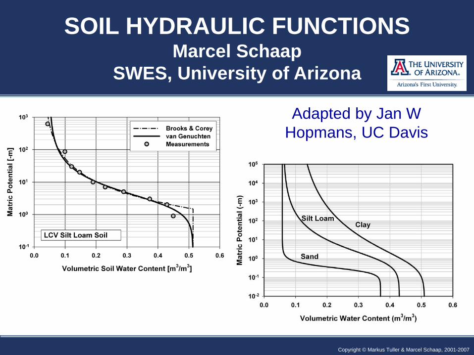
Copyright © Markus Tuller & Marcel Schaap, 2001-2007 SOIL HYDRAULIC FUNCTIONS Marcel Schaap SWES, University of Arizona Adapted by Jan W Hopmans, UC Davis
Transcript of SOIL HYDRAULIC FUNCTIONS - Jan Hopmans
Copyright © Markus Tuller, 2006 Copyright © Markus Tuller & Marcel Schaap, 2001-2007
SOIL HYDRAULIC FUNCTIONS Marcel Schaap
SWES, University of Arizona
Adapted by Jan W Hopmans, UC Davis
Copyright © Markus Tuller, 2006 Copyright © Markus Tuller & Marcel Schaap, 2001-2007
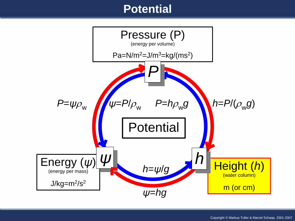
Potential
Energy (ψ) (energy per mass)
J/kg=m2/s2
ψ
h=P/(ρwg) P=hρwg P=ψρw ψ=P/ρw
ψ=hg
h=ψ/g
Pressure (P) (energy per volume)
Pa=N/m2=J/m3=kg/(ms2)
Height (h) (water column)
m (or cm)
Potential
h
P
Copyright © Markus Tuller, 2006 Copyright © Markus Tuller & Marcel Schaap, 2001-2007
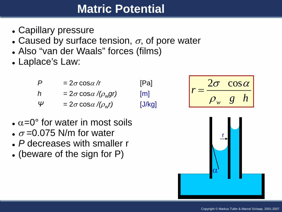
Capillary pressure Caused by surface tension, σ, of pore water Also “van der Waals” forces (films) Laplace’s Law:
P = 2σ cosα /r [Pa] h = 2σ cosα /(ρwgr) [m] Ψ = 2σ cosα /(ρwr) [J/kg] α=0° for water in most soils σ =0.075 N/m for water P decreases with smaller r (beware of the sign for P) α
r
Matric Potential
2 cos
w
rg h
σ αρ
=
Copyright © Markus Tuller, 2006 Copyright © Markus Tuller & Marcel Schaap, 2001-2007
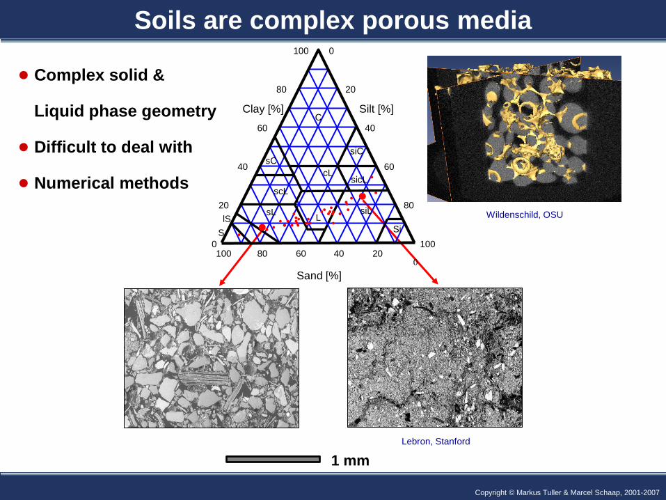
Soils are complex porous media
● Complex solid &
Liquid phase geometry
● Difficult to deal with
● Numerical methods
1 mm
0
100 0
20
80 20
40
60 40
60
40 60
80
20 80
100 0 100
Clay [%] Silt [%]
Sand [%]
S lS
sL L siL
Si
scL
cL sicL
siC sC
C
Wildenschild, OSU
Lebron, Stanford
Copyright © Markus Tuller, 2006 Copyright © Markus Tuller & Marcel Schaap, 2001-2007
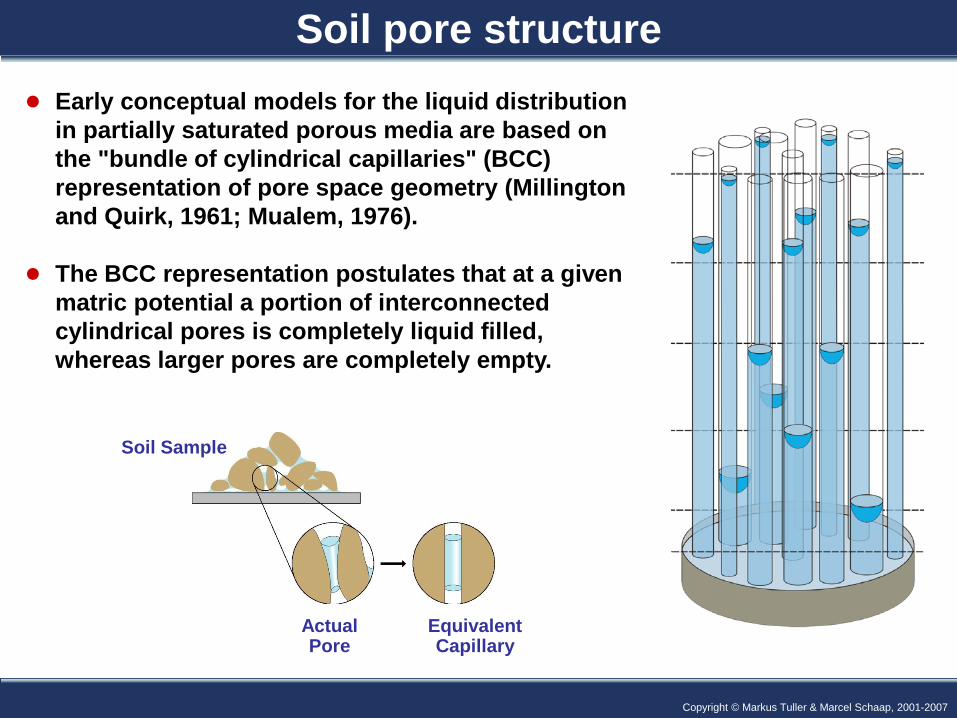
Soil pore structure ● Early conceptual models for the liquid distribution
in partially saturated porous media are based on the "bundle of cylindrical capillaries" (BCC) representation of pore space geometry (Millington and Quirk, 1961; Mualem, 1976).
● The BCC representation postulates that at a given
matric potential a portion of interconnected cylindrical pores is completely liquid filled, whereas larger pores are completely empty.
Soil Sample
Actual Pore
Equivalent Capillary
Copyright © Markus Tuller, 2006 Copyright © Markus Tuller & Marcel Schaap, 2001-2007
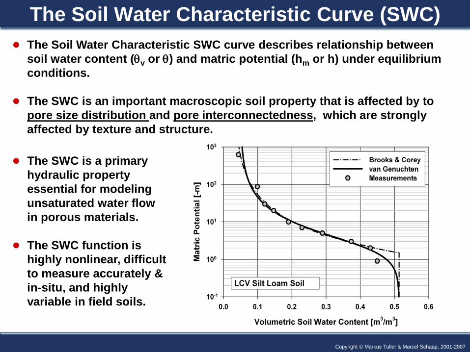
The Soil Water Characteristic Curve (SWC) ● The Soil Water Characteristic SWC curve describes relationship between
soil water content (θv or θ) and matric potential (hm or h) under equilibrium conditions.
● The SWC is an important macroscopic soil property that is affected by to pore size distribution and pore interconnectedness, which are strongly affected by texture and structure.
● The SWC is a primary hydraulic property essential for modeling unsaturated water flow in porous materials.
● The SWC function is highly nonlinear, difficult to measure accurately & in-situ, and highly variable in field soils.
Copyright © Markus Tuller, 2006 Copyright © Markus Tuller & Marcel Schaap, 2001-2007
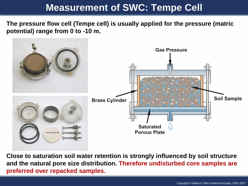
Measurement of SWC: Tempe Cell The pressure flow cell (Tempe cell) is usually applied for the pressure (matric potential) range from 0 to -10 m.
Close to saturation soil water retention is strongly influenced by soil structure and the natural pore size distribution. Therefore undisturbed core samples are preferred over repacked samples.
Copyright © Markus Tuller, 2006 Copyright © Markus Tuller & Marcel Schaap, 2001-2007
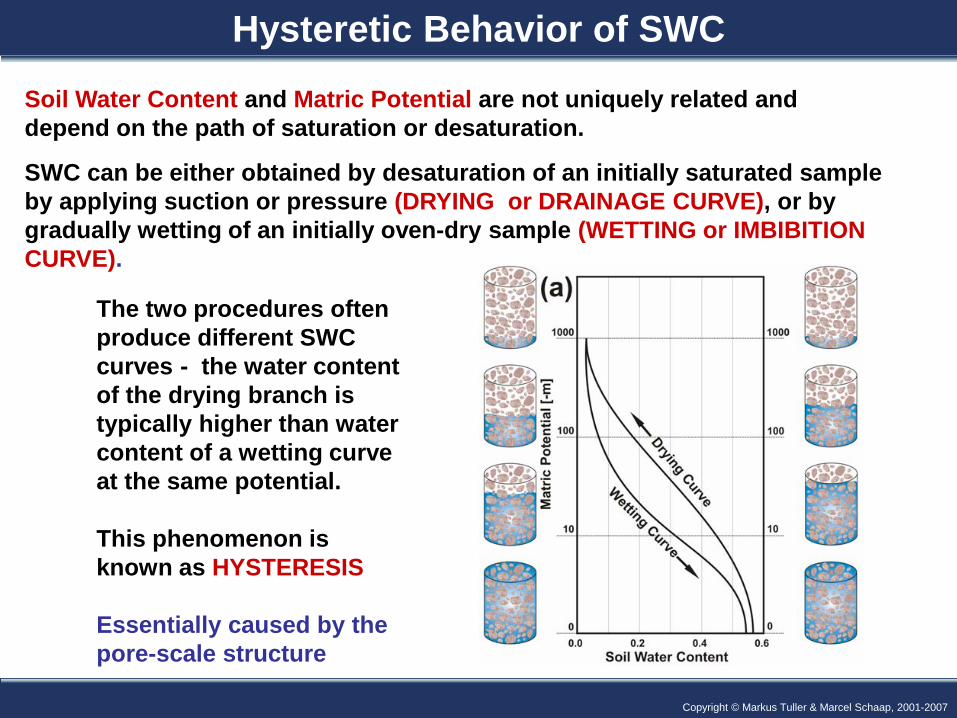
Hysteretic Behavior of SWC
Soil Water Content and Matric Potential are not uniquely related and depend on the path of saturation or desaturation.
SWC can be either obtained by desaturation of an initially saturated sample by applying suction or pressure (DRYING or DRAINAGE CURVE), or by gradually wetting of an initially oven-dry sample (WETTING or IMBIBITION CURVE).
The two procedures often produce different SWC curves - the water content of the drying branch is typically higher than water content of a wetting curve at the same potential. This phenomenon is known as HYSTERESIS Essentially caused by the pore-scale structure
Copyright © Markus Tuller, 2006 Copyright © Markus Tuller & Marcel Schaap, 2001-2007
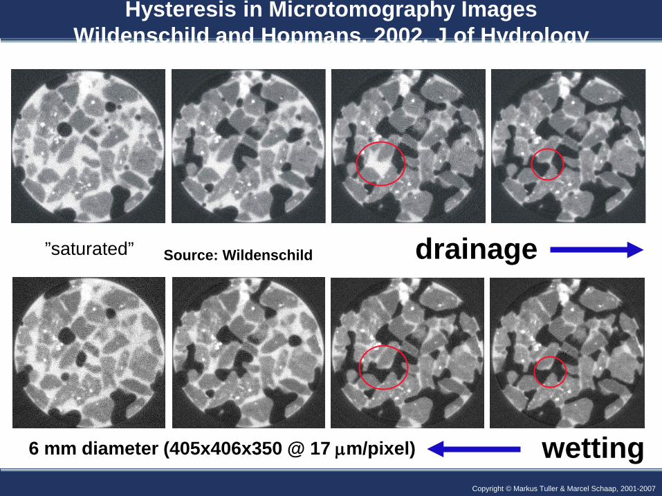
Hysteresis in Microtomography Images Wildenschild and Hopmans, 2002, J of Hydrology
drainage ”saturated”
wetting 6 mm diameter (405x406x350 @ 17 µm/pixel)
Source: Wildenschild
Copyright © Markus Tuller, 2006 Copyright © Markus Tuller & Marcel Schaap, 2001-2007
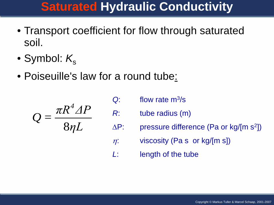
Saturated Hydraulic Conductivity
• Transport coefficient for flow through saturated soil.
• Symbol: Ks
• Poiseuille's law for a round tube:
8
4πR ΔPQ =ηL
Q: flow rate m3/s
R: tube radius (m)
∆P: pressure difference (Pa or kg/[m s2])
η: viscosity (Pa s or kg/[m s])
L: length of the tube
Copyright © Markus Tuller, 2006 Copyright © Markus Tuller & Marcel Schaap, 2001-2007
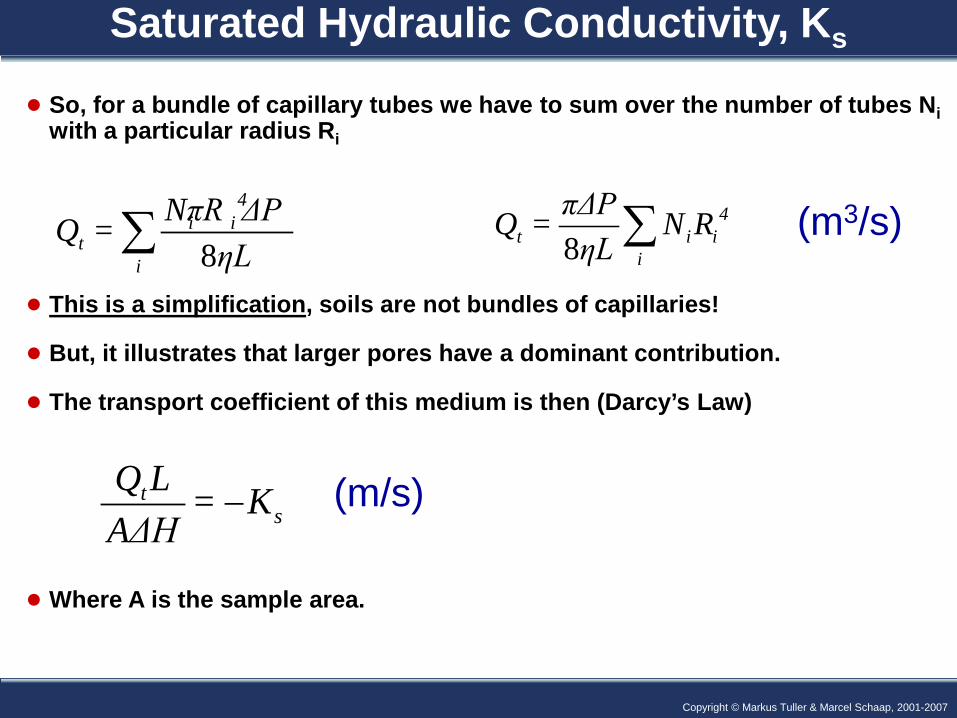
● So, for a bundle of capillary tubes we have to sum over the number of tubes Ni with a particular radius Ri
8
4i i
ti
NπR ΔPQ =ηL∑
Saturated Hydraulic Conductivity, Ks
84
t i ii
πΔPQ = N RηL ∑
● This is a simplification, soils are not bundles of capillaries!
● But, it illustrates that larger pores have a dominant contribution.
● The transport coefficient of this medium is then (Darcy’s Law)
t
sQ L = KAΔH
−
● Where A is the sample area.
(m3/s)
(m/s)
Copyright © Markus Tuller, 2006 Copyright © Markus Tuller & Marcel Schaap, 2001-2007
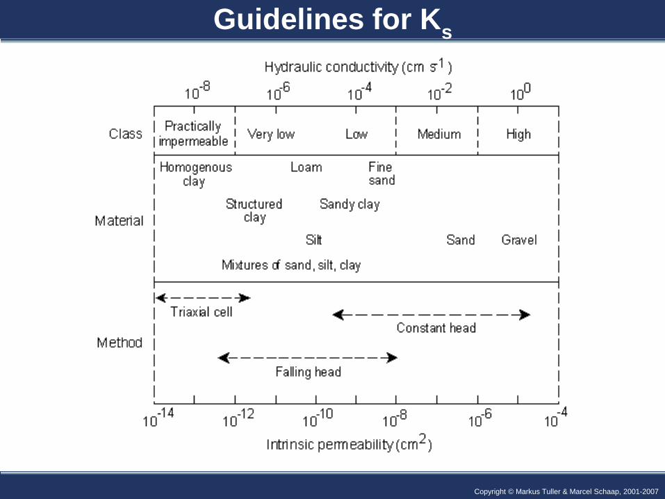
Guidelines for Ks
Copyright © Markus Tuller, 2006 Copyright © Markus Tuller & Marcel Schaap, 2001-2007
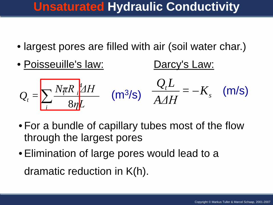
Unsaturated Hydraulic Conductivity
8
4i i
ti
NπR ΔHQ =ηL∑
• largest pores are filled with air (soil water char.)
• Poisseuille's law: Darcy's Law:
• For a bundle of capillary tubes most of the flow through the largest pores
• Elimination of large pores would lead to a
dramatic reduction in K(h).
ts
Q L = KAΔH
−(m3/s) (m/s)
Copyright © Markus Tuller, 2006 Copyright © Markus Tuller & Marcel Schaap, 2001-2007
0.00001
0.0001
0.001
0.01
0.1
1
10
100
1000
10000
100000
0.1 1 10 100 1000 10000
- Capillary head (cm)
Con
duct
ivity
(cm
/day
)
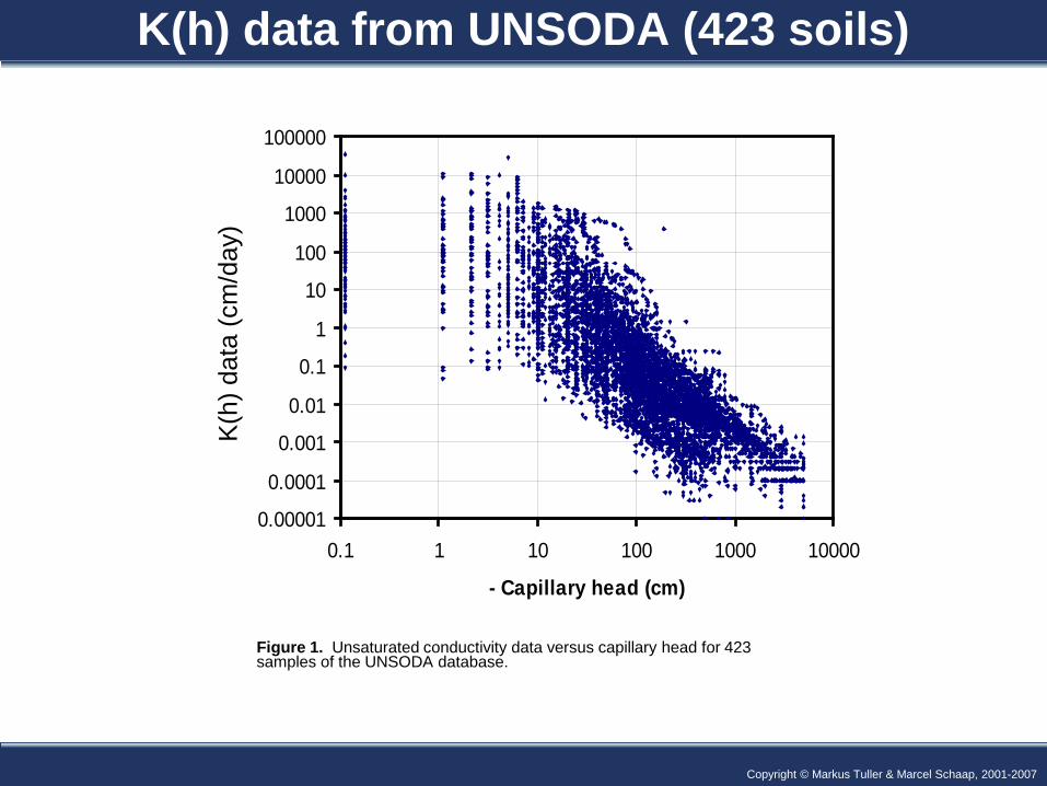
Figure 1. Unsaturated conductivity data versus capillary head for 423 samples of the UNSODA database.
K(h
) dat
a (c
m/d
ay)
K(h) data from UNSODA (423 soils)
Copyright © Markus Tuller, 2006 Copyright © Markus Tuller & Marcel Schaap, 2001-2007
0 0.1 0.2 0.3 0.4 0.5 1
10
102
103
104
Water content (cm3/cm3)
-Mat
ric h
ead
(cm
)
Loam
Sand
0 0.2 0.4 0.6 0.8 1
10-5
10-3
0.1
10
103
Relative saturation, Se
log
K (
cm/d
ay)
Loam
Sand
0 10 102 103 104 105
10-5
10-3
0.1
10
103
-Matric head (cm)
log
K [
cm/d
ay]
Loam
Sand
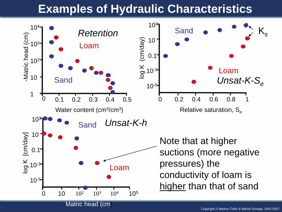
Note that at higher suctions (more negative pressures) the conductivity of loam is higher than that of sand
Ks Retention
Unsat-K-Se
Unsat-K-h
Examples of Hydraulic Characteristics
Copyright © Markus Tuller, 2006 Copyright © Markus Tuller & Marcel Schaap, 2001-2007
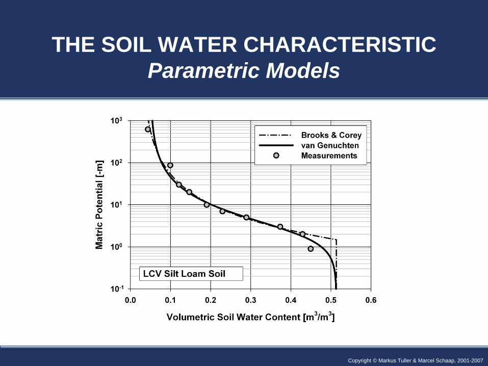
THE SOIL WATER CHARACTERISTIC Parametric Models
Copyright © Markus Tuller, 2006 Copyright © Markus Tuller & Marcel Schaap, 2001-2007
Parametric Models
• Measuring soil hydraulic properties is laborious and time consuming and expensive. Usually there are only a few data pairs available from measurements. • For modeling and analysis (characterization and comparison of different soils) it is beneficial to represent the hydraulic relationships as continuous parametric functions. • Commonly used parametric models are the van Genuchten and Brooks & Corey relationships. Other models are Kosugi lognormal and Campbell model. • We like to use specific equations rather than splines (or other mathematical ways to describe/interpolate data) because the equation parameters can be interpreted or communicated.
● No “true” SWC model defined based on (microscopically ) observed pore size distributions.
Copyright © Markus Tuller, 2006 Copyright © Markus Tuller & Marcel Schaap, 2001-2007
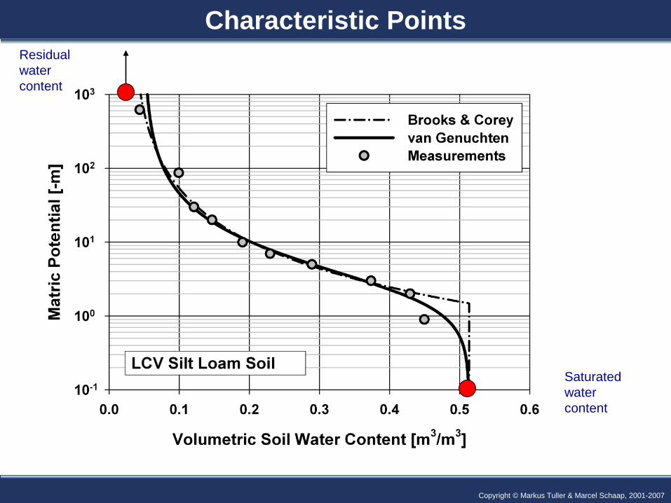
Characteristic Points
Saturated water content
Residual water content
Copyright © Markus Tuller, 2006 Copyright © Markus Tuller & Marcel Schaap, 2001-2007
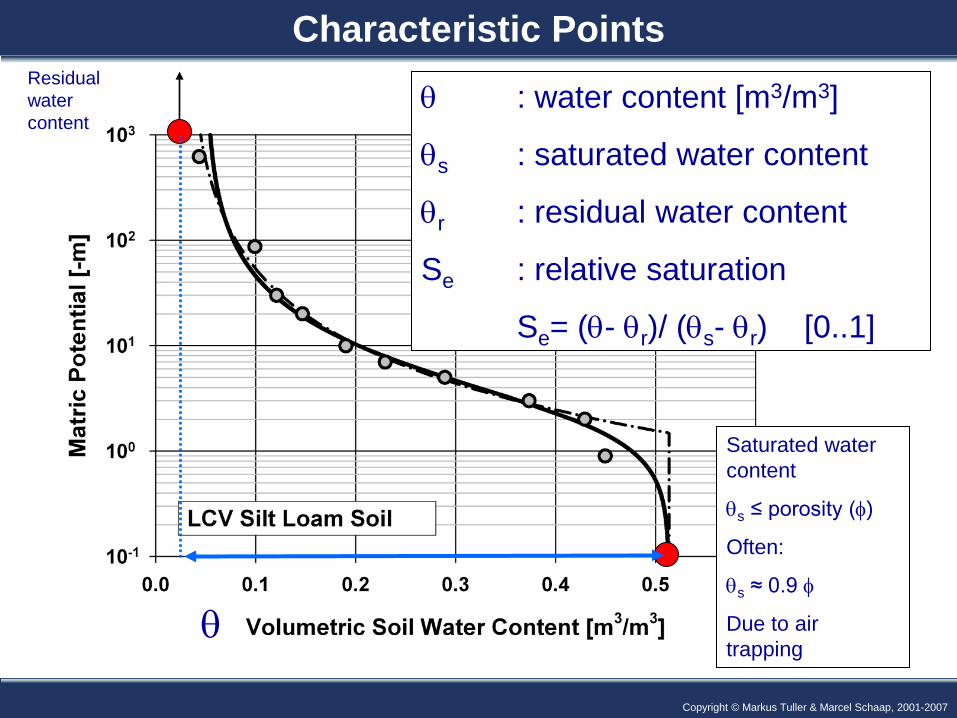
Characteristic Points
Saturated water content
θs ≤ porosity (φ)
Often:
θs ≈ 0.9 φ
Due to air trapping
Residual water content
θ : water content [m3/m3]
θs : saturated water content
θr : residual water content
Se : relative saturation
Se= (θ- θr)/ (θs- θr) [0..1]
θ
Copyright © Markus Tuller, 2006 Copyright © Markus Tuller & Marcel Schaap, 2001-2007
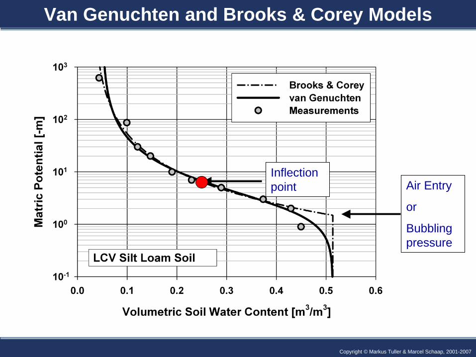
Van Genuchten and Brooks & Corey Models
Air Entry
or
Bubbling pressure
Inflection point
Copyright © Markus Tuller, 2006 Copyright © Markus Tuller & Marcel Schaap, 2001-2007
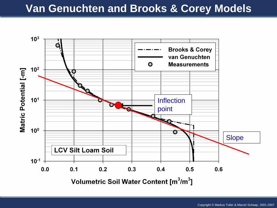
Van Genuchten and Brooks & Corey Models
Inflection point
Slope
Copyright © Markus Tuller, 2006 Copyright © Markus Tuller & Marcel Schaap, 2001-2007
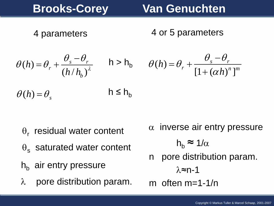
( )[1 ( ) ]
s rr n mh
hθ θθ θ
α−
= ++
4 parameters 4 or 5 parameters
θr residual water content
θs saturated water content
hb air entry pressure
λ pore distribution param.
( )( / )
s rr
b
hh h λ
θ θθ θ −= +
α inverse air entry pressure
hb ≈ 1/α n pore distribution param. λ≈n-1 m often m=1-1/n
( ) shθ θ=
h > hb
h ≤ hb
Brooks-Corey Van Genuchten
Copyright © Markus Tuller, 2006 Copyright © Markus Tuller & Marcel Schaap, 2001-2007
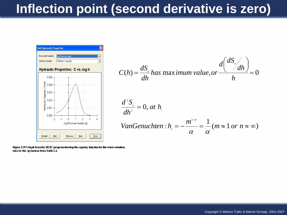
Inflection point (second derivative is zero)
0,max)( =
=h
dhdSd
orvalueimumhasdhdShC
e
e
)1(1:
,01
2
2
∞≈≈=−=
=
−
normmhenVanGenucht
hatdh
Sd
m
i
ie
αα
Copyright © Markus Tuller, 2006 Copyright © Markus Tuller & Marcel Schaap, 2001-2007
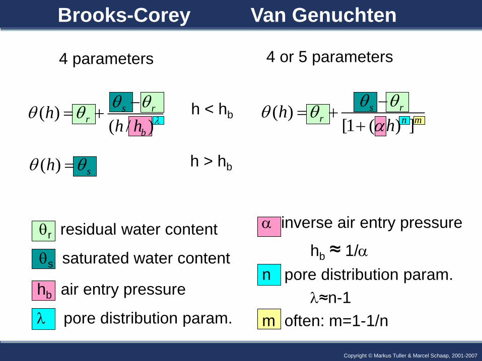
( )[1 ( ) ]
s rr n mh
hθ θθ θ
α−
= ++
4 parameters 4 or 5 parameters
θr residual water content
θs saturated water content
hb air entry pressure
λ pore distribution param.
( )( / )
s rr
b
hh h λ
θ θθ θ −= +
α inverse air entry pressure
hb ≈ 1/α n pore distribution param. λ≈n-1 m often: m=1-1/n
( ) shθ θ=
h < hb
h > hb
Brooks-Corey Van Genuchten
Copyright © Markus Tuller, 2006 Copyright © Markus Tuller & Marcel Schaap, 2001-2007
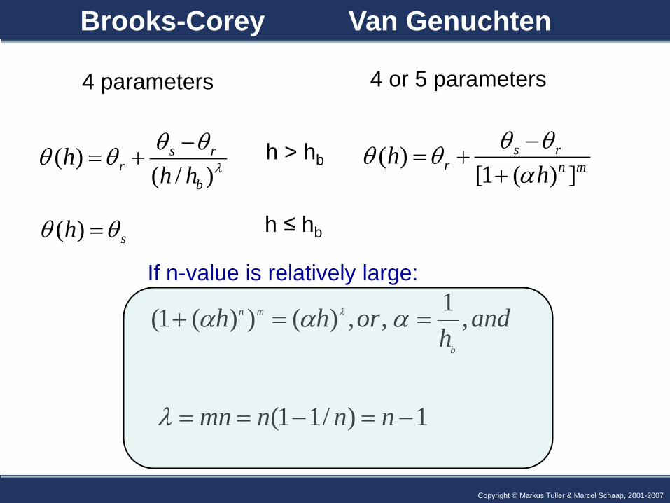
( )[1 ( ) ]
s rr n mh
hθ θθ θ
α−
= ++
4 parameters 4 or 5 parameters
( )( / )
s rr
b
hh h λ
θ θθ θ −= +
( ) shθ θ=
h > hb
h ≤ hb
Brooks-Corey Van Genuchten
1)/11(
,1,,)())(1(
−=−==
==+
nnnmn
andh
orhhb
mn
λ
ααα λ
If n-value is relatively large:
Copyright © Markus Tuller, 2006 Copyright © Markus Tuller & Marcel Schaap, 2001-2007
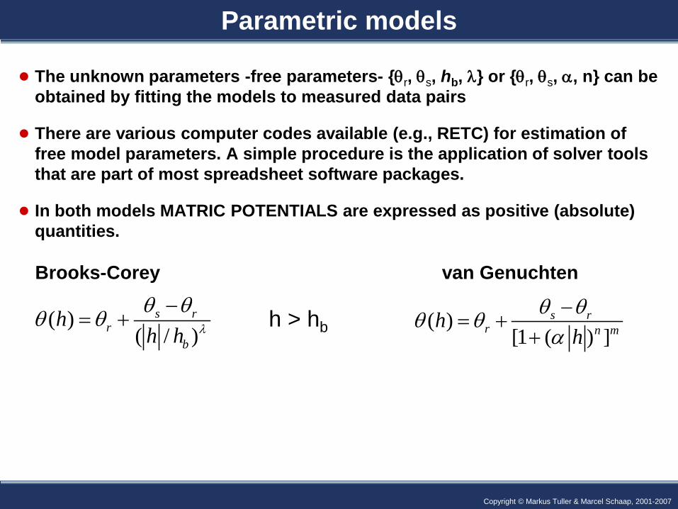
Parametric models
● The unknown parameters -free parameters- {θr, θs, hb, λ} or {θr, θs, α, n} can be obtained by fitting the models to measured data pairs
● There are various computer codes available (e.g., RETC) for estimation of free model parameters. A simple procedure is the application of solver tools that are part of most spreadsheet software packages.
● In both models MATRIC POTENTIALS are expressed as positive (absolute) quantities.
( )[1 ( ) ]
s rr n mh
hθ θθ θ
α−
= ++
h > hb
Brooks-Corey van Genuchten
( )( / )
s rr
b
hh h λ
θ θθ θ −= +
Copyright © Markus Tuller, 2006 Copyright © Markus Tuller & Marcel Schaap, 2001-2007
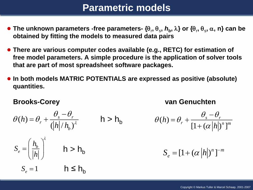
Parametric models
● The unknown parameters -free parameters- {θr, θs, hb, λ} or {θr, θs, α, n} can be obtained by fitting the models to measured data pairs
● There are various computer codes available (e.g., RETC) for estimation of free model parameters. A simple procedure is the application of solver tools that are part of most spreadsheet software packages.
● In both models MATRIC POTENTIALS are expressed as positive (absolute) quantities.
( )[1 ( ) ]
s rr n mh
hθ θθ θ
α−
= ++
be
hSh
λ
=
h > hb
Brooks-Corey van Genuchten
( )( / )
s rr
b
hh h λ
θ θθ θ −= +
[1 ( ) ]n meS hα −= +h > hb
1eS = h ≤ hb
Copyright © Markus Tuller, 2006 Copyright © Markus Tuller & Marcel Schaap, 2001-2007
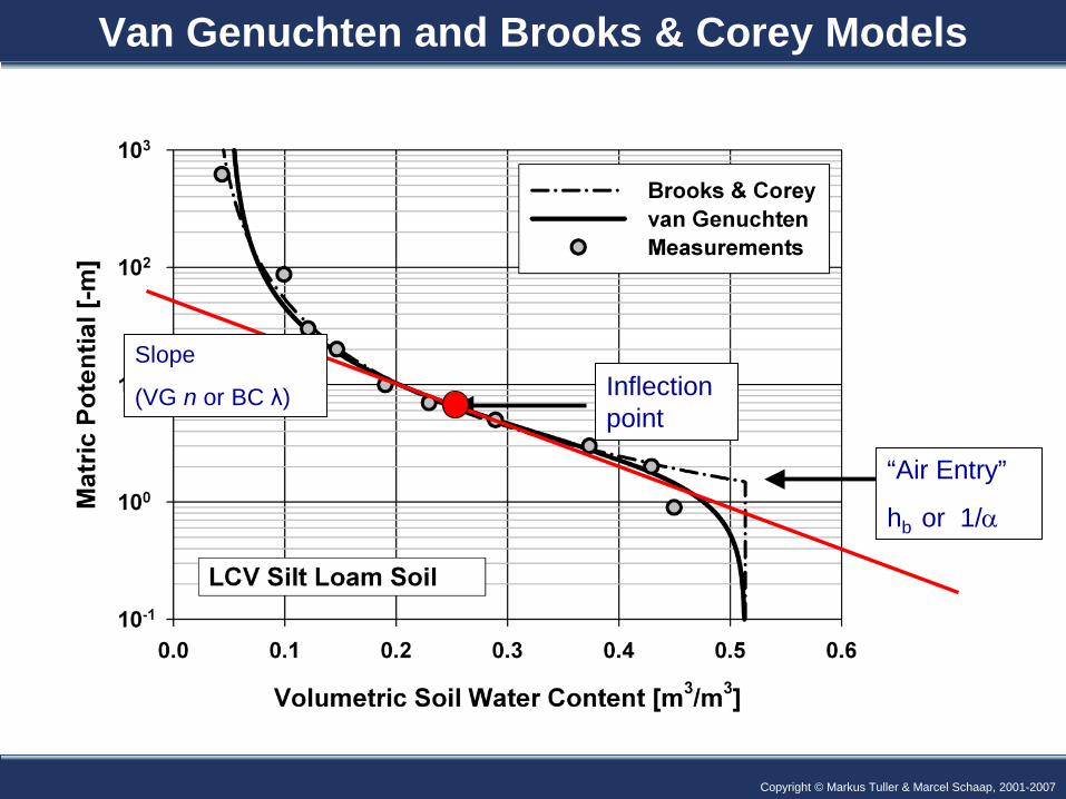
Van Genuchten and Brooks & Corey Models
Inflection point
Slope
(VG n or BC λ)
“Air Entry”
hb or 1/α
Copyright © Markus Tuller, 2006 Copyright © Markus Tuller & Marcel Schaap, 2001-2007
1.0E+00
1.0E+01
1.0E+02
1.0E+03
1.0E+04
1.0E+05
0 0.1 0.2 0.3 0.4 0.5
Water content (cm3/cm3)
Pres
sure
, h (c
m) n=1.2
n=1.5n=2n=3n=5
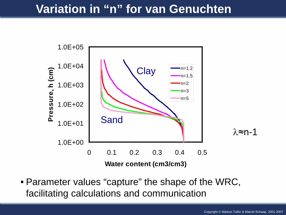
• Parameter values “capture” the shape of the WRC, facilitating calculations and communication
Variation in “n” for van Genuchten
λ≈n-1 Sand
Clay
Copyright © Markus Tuller, 2006 Copyright © Markus Tuller & Marcel Schaap, 2001-2007
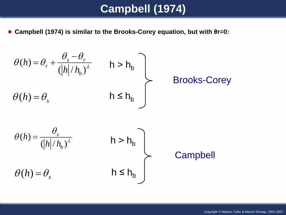
Campbell (1974)
● Campbell (1974) is similar to the Brooks-Corey equation, but with θr=0:
( )( / )
s
b
hh h λ
θθ = h > hb
( )( / )
s rr
b
hh h λ
θ θθ θ −= +
Brooks-Corey
( ) shθ θ= h ≤ hb
Campbell
( ) shθ θ= h ≤ hb
h > hb
Copyright © Markus Tuller, 2006 Copyright © Markus Tuller & Marcel Schaap, 2001-2007
Physically-based models
● All parametric SWC models are empirical: they are successful because they describe observed θ-h data well (for certain soils)
● No “true” SWC model defined based on (microscopically ) observed pore size distributions.
● However, it is often observed that soil particle sizes are “log-normally” distributed.
● Assuming that:
this implies a log-normal size distribution of pore-volume pores are cylindrical
● We can define what a SWC should look like.
● Arya and Paris (actually distribution-free, not in this lecture)
● Kosugi model
Copyright © Markus Tuller, 2006 Copyright © Markus Tuller & Marcel Schaap, 2001-2007
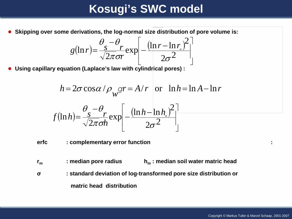
Kosugi’s SWC model
● Skipping over some derivations, the log-normal size distribution of pore volume is:
● Using capillary equation (Laplace’s law with cylindrical pores) :
erfc : complementary error function :
rm : median pore radius hm : median soil water matric head
σ : standard deviation of log-transformed pore size distribution or
matric head distribution
This image cannot currently be displayed.
rAhrArwh lnlnlnor //cos2 −=== gρασ
( ) ( )
−−−
= 22
2lnlnexp2
lnσσπ
θθmhh
hrshf
( ) ( )
−−−
= 22
2lnlnexp2
lnσσπ
θθmrr
rrsrg
Copyright © Markus Tuller, 2006 Copyright © Markus Tuller & Marcel Schaap, 2001-2007
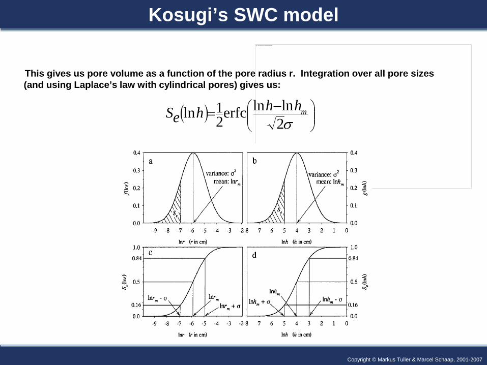
Kosugi’s SWC model
This gives us pore volume as a function of the pore radius r. Integration over all pore sizes (and using Laplace’s law with cylindrical pores) gives us:
This image cannot currently be displayed.
( )
−=σ2lnlnerfc2
1ln mhhheS
Copyright © Markus Tuller, 2006 Copyright © Markus Tuller & Marcel Schaap, 2001-2007
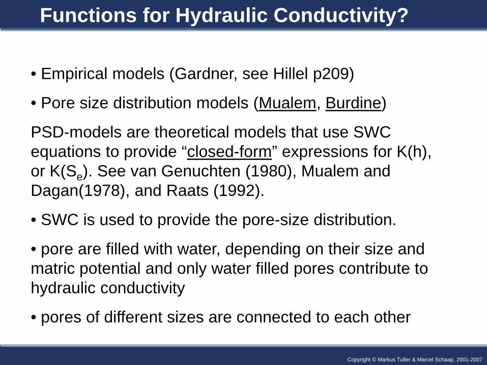
• Empirical models (Gardner, see Hillel p209)
• Pore size distribution models (Mualem, Burdine)
PSD-models are theoretical models that use SWC equations to provide “closed-form” expressions for K(h), or K(Se). See van Genuchten (1980), Mualem and Dagan(1978), and Raats (1992).
• SWC is used to provide the pore-size distribution.
• pore are filled with water, depending on their size and matric potential and only water filled pores contribute to hydraulic conductivity
• pores of different sizes are connected to each other
Functions for Hydraulic Conductivity?
Copyright © Markus Tuller, 2006 Copyright © Markus Tuller & Marcel Schaap, 2001-2007
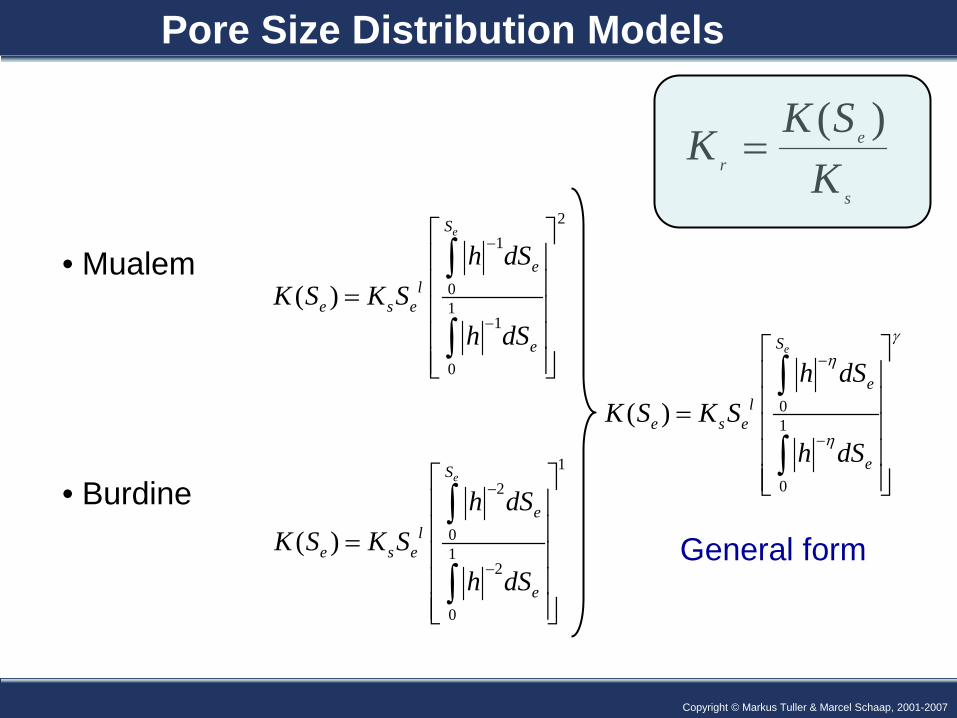
• Mualem
• Burdine
Pore Size Distribution Models
21
01
1
0
( )
eS
el
e s e
e
h dSK S K S
h dS
−
−
=
∫
∫
12
01
2
0
( )
eS
el
e s e
e
h dSK S K S
h dS
−
−
=
∫
∫
01
0
( )
eS
el
e s e
e
h dSK S K S
h dS
γη
η
−
−
=
∫
∫
General form
s
er K
SKK )(=
Copyright © Markus Tuller, 2006 Copyright © Markus Tuller & Marcel Schaap, 2001-2007
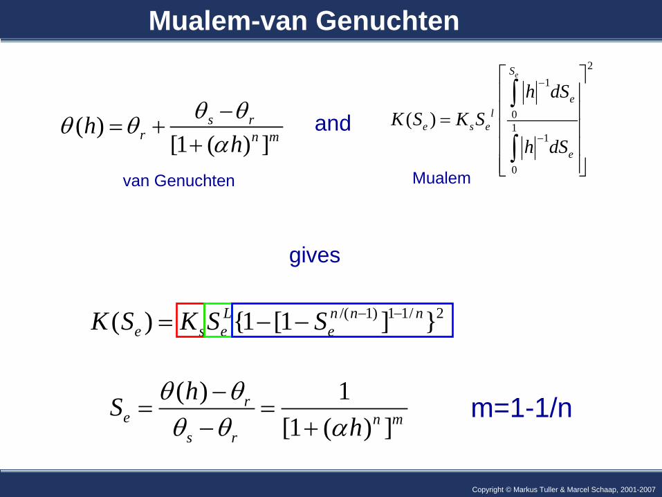
/( 1) 1 1/ 2( ) {1 [1 ] }L n n ne s e eK S K S S − −= − −
Mualem-van Genuchten
( ) 1[1 ( ) ]
re n m
s r
hSh
θ θθ θ α
−= =
− +m=1-1/n
( )[1 ( ) ]
s rr n mh
hθ θθ θ
α−
= ++
21
01
1
0
( )
eS
el
e s e
e
h dSK S K S
h dS
−
−
=
∫
∫and
gives
van Genuchten Mualem
Copyright © Markus Tuller, 2006 Copyright © Markus Tuller & Marcel Schaap, 2001-2007
/( 1) 1 1/ 2( ) {1 [1 ] }L n n ne s e eK S K S S − −= − −
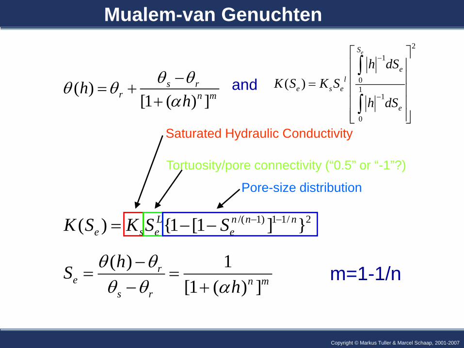
Mualem-van Genuchten
( ) 1[1 ( ) ]
re n m
s r
hSh
θ θθ θ α
−= =
− +
Saturated Hydraulic Conductivity
Tortuosity/pore connectivity (“0.5” or “-1”?)
Pore-size distribution
m=1-1/n
( )[1 ( ) ]
s rr n mh
hθ θθ θ
α−
= ++
21
01
1
0
( )
eS
el
e s e
e
h dSK S K S
h dS
−
−
=
∫
∫and
Copyright © Markus Tuller, 2006 Copyright © Markus Tuller & Marcel Schaap, 2001-2007
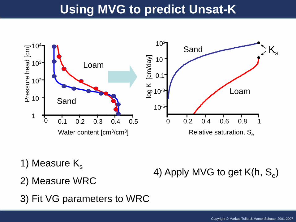
0 0.1 0.2 0.3 0.4 0.5 1
10
102
103
104
Water content [cm3/cm3]
Pre
ssur
e he
ad [c
m]
Loam
Sand
0 0.2 0.4 0.6 0.8 1
10-5
10-3
0.1
10
103
Relative saturation, Se
log
K [
cm/d
ay]
Loam
Sand Ks
1) Measure Ks
2) Measure WRC
3) Fit VG parameters to WRC
4) Apply MVG to get K(h, Se)
Using MVG to predict Unsat-K
Copyright © Markus Tuller, 2006 Copyright © Markus Tuller & Marcel Schaap, 2001-2007
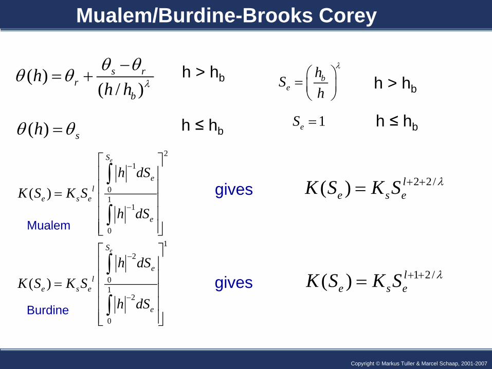
2 2/( ) le s eK S K S λ+ +=
Mualem/Burdine-Brooks Corey
21
01
1
0
( )
eS
el
e s e
e
h dSK S K S
h dS
−
−
=
∫
∫gives
Mualem
( )( / )
s rr
b
hh h λ
θ θθ θ −= +
( ) shθ θ=
h > hb
h ≤ hb
be
hSh
λ =
h > hb
1eS = h ≤ hb
12
01
2
0
( )
eS
el
e s e
e
h dSK S K S
h dS
−
−
=
∫
∫Burdine
1 2/( ) le s eK S K S λ+ +=gives
Copyright © Markus Tuller, 2006 Copyright © Markus Tuller & Marcel Schaap, 2001-2007
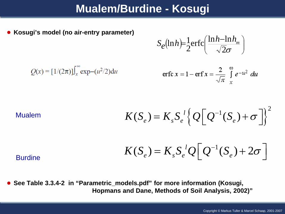
Mualem/Burdine - Kosugi
● Kosugi’s model (no air-entry parameter)
● See Table 3.3.4-2 in “Parametric_models.pdf” for more information (Kosugi, Hopmans and Dane, Methods of Soil Analysis, 2002)”
{ }21( ) ( )le s e eK S K S Q Q S σ− = + Mualem
1( ) ( ) 2le s e eK S K S Q Q S σ− = + Burdine
( )
−=σ2lnlnerfc2
1ln mhhheS
Copyright © Markus Tuller, 2006 Copyright © Markus Tuller & Marcel Schaap, 2001-2007
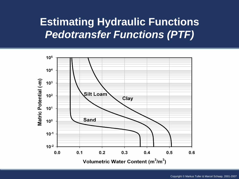
Estimating Hydraulic Functions Pedotransfer Functions (PTF)