SOBOLEV DUALS IN FRAME THEORY AND SIGMA-DELTA …

SOBOLEV DUALS IN FRAME THEORY ANDSIGMA-DELTA QUANTIZATION

JAMES BLUM, MARK LAMMERS, ALEXANDER M. POWELL, AND OZGUR YILMAZ

Abstract. A new class of alternative dual frames is introduced in the settingof finite frames for Rd. These dual frames, called Sobolev duals, provide a high

precision linear reconstruction procedure for Sigma-Delta (Σ∆) quantizationof finite frames. The main result is summarized as follows: reconstruction with

Sobolev duals enables stable rth order Sigma-Delta schemes to achieve deter-

ministic approximation error of order O(N−r) for a wide class of finite framesof size N . This asymptotic order is generally not achievable with canonical

dual frames. Moreover, Sobolev dual reconstruction leads to minimal mean

squared error under the classical white noise assumption.

1. Introduction

In signal processing, an essential problem is to encode a signal, typically an ana-log object, with finitely many bits in an efficient and robust manner. Efficiency ofan encoding is reflected by the associated approximation error: given a bit-budget,one seeks the error to be as small as possible in an appropriate norm. Noting thatthe encoding process typically involves an analog-to-digital (A/D) conversion step,it is also essential that the required digital representation be robust, for example,with respect to errors in arithmetic operations during the encoding process, andpartial loss of information. This robustness requirement is frequently satisfied byredundantly representing signals before the A/D conversion or quantization stage.For example, one oversamples if the signals to be encoded are bandlimited func-tions, or one uses overcomplete frame expansions if the signals of interest are vectorsin a finite dimensional Hilbert space.

Redundantly representing a signal provides robustness, but it also makes A/Dconversion more complex since coefficients in the representation are correlated. Inparticular, componentwise scalar quantization, also known as pulse code modulation(PCM), is generally suboptimal for redundant expansions. Σ∆ quantization wasdevised as an alternative to PCM for quantizing bandlimited sampling expansions,[19]. Since then, the practice has matured and Σ∆ quantizers have establishedthemselves as a preferred method for quantizing oversampled bandlimited signals,e.g., see [23]. The mathematical theory of Σ∆ quantization on the other handis quite recent. After work by Gray, e.g., [14, 16], Daubechies and DeVore [10]established an approximation theoretical framework and provided rigorous resultson the relationship between robustness of Σ∆ schemes, redundancy of the associatedrepresentations, and the approximation error. The work in [10] gives an explicitconstruction of stable 1-bit Σ∆ schemes of general order r. Moreover, [10] shows

M. Lammers was supported in part by a Cahill Grant from UNCW.A.M. Powell was supported in part by NSF Grant DMS-0811086.

O. Yılmaz was supported in part by NSERC of Canada.

1

2 J. BLUM, M. LAMMERS, A.M. POWELL, AND O. YILMAZ

that in the bandlimited setting the L∞ approximation error associated with a stablerth order Σ∆ scheme behaves like 1/λr where λ is the oversampling ratio.

Inspired by the work of Daubechies and DeVore, in particular that Σ∆ quantiza-tion exploits redundancy more efficiently than PCM for bandlimited functions, [2]investigated the use of Σ∆ quantization for redundant finite frame expansions. Theperformance of PCM for quantizing finite frames is well investigated, e.g., [13, 12].It was shown in [2] that even a first order Σ∆ scheme outperforms PCM (withlinear reconstruction) in terms of approximation error, at least for certain familiesof frames with sufficiently high redundancy.

A main focus of the subsequent work in [1, 7, 4, 5, 21] is to achieve betterapproximation rates (as the redundancy of the frame increases) for higher orderΣ∆ schemes. In particular, one desires an approximation error of order O(N−r)with an rth order Σ∆ scheme, where N is the number of frame vectors. It wasproved in [21] that for Σ∆ schemes of order 3 or higher one cannot obtain thesesought-for approximation rates, at least in the case of harmonic frames, if one usescanonical dual frames in the reconstruction. As a remedy, two main approaches havebeen developed. One approach concentrates on choosing special Parseval framesand uses the same frame in both analysis and reconstruction after quantization,e.g., [5]. This approach is less computationally intensive as there is no need tocompute a dual frame, but it only works for rather specific analysis frames. Adifferent approach used in [21], and in this paper, allows a more flexible choice ofanalysis frame and chooses a non-canonical dual frame that is specially designedfor the particular quantization scheme.

Overview. The work in [21] identifies general conditions under which alternativedual frames can be used in rth order Σ∆ quantization to achieve pointwise recon-struction error of order O(N−r), where N is the frame size. However, [21] does notindicate how to construct such alternative dual frames. Indeed, concrete examplesare only given for harmonic frames and the methods are decidedly ad hoc.

The main result of this paper, Theorem 5.4, provides a general constructivemethod for finding alternative dual frames that are suitable for reconstruction inhigher order Σ∆ quantization of finite frames. Specifically, we define a new classof alternative dual frames, the Sobolev duals, and prove that the associated recon-struction error for rth order Σ∆ quantization satisfies ||x− x|| = O(N−r).

The paper is organized as follows. Section 2 recalls basic frame theory. Section3 briefly reviews Σ∆ quantization for finite frames. In Section 4 we define Sobolevdual frames. Our main result, Theorem 5.4, on pointwise Σ∆ error bounds withSobolev duals is proven in Section 5. Section 6 addresses mean squared error withSobolev duals. Section 7 contains numerical results.

2. Finite frames

Definition 2.1. A finite collection of vectors {en}Nn=1 ⊆ Rd is a frame for Rd withframes bounds 0 < A ≤ B <∞ if

(2.1) ∀x ∈ Rd, A‖x‖2 ≤N∑n=1

|〈x, en〉|2 ≤ B‖x‖2,

SOBOLEV DUALS IN FRAME THEORY AND SIGMA-DELTA QUANTIZATION 3

where ‖ · ‖ = ‖ · ‖2 denotes the Euclidean norm. If A = B then the frame is said tobe tight, and it is unit-norm if ‖en‖ = 1 for each n. The frame bounds are takento be the respective largest and smallest values of A and B such that (2.1) holds.

If {en}Nn=1 ⊆ Rd is a frame then there exists a dual frame {fn}Nn=1 ⊆ Rd suchthat

(2.2) ∀x ∈ Rd, x =N∑n=1

〈x, en〉fn =N∑n=1

〈x, fn〉en.

If N > d then the frame {en}Nn=1 ⊂ Rd is an overcomplete collection and the choiceof dual frame {fn}Nn=1 in (2.2) is not unique. We will work with the left expansionin (2.2), and hence refer to {en}Nn=1 as the analysis or encoding frame, and the dualframe {fn}Nn=1 as the synthesis or decoding frame. Tight frames have the propertythat the dual frame can be chosen as fn = A−1en, where A is the frame bound.For more background on frames see [8, 9].

For finite frames in Rd, the basic definitions can be conveniently reformulatedin terms of matrices. Given a frame {en}Nn=1 ⊂ Rd we define the associated framematrix E to be the d × N matrix with ej as its jth column. In particular, thecolumns of a d×N matrix E form a frame for Rd if and only if E has rank d. Inview of this equivalence, we shall identify a frame {en}Nn=1 with its frame matrix Eand simply refer to both as frames for Rd.

Let {en}Nn=1 ⊂ Rd be a frame for Rd with dual frame {fn}Nn=1 ⊂ Rd, and let Eand F be the corresponding d×N frame matrices. The frame expansions (2.2) canbe equivalently expressed in terms of E and F as

FE∗ = EF ∗ = Id,

where Id is the d × d identity matrix and S∗ denotes the adjoint of a matrix S.Namely, F is a dual frame for E if and only if F is a left inverse to E∗. This naturallyleads one to define the canonical dual frame associated to E by F = (EE∗)−1E.The canonical dual frame is a minimal norm dual frame with respect to variousmatrix norms described below.

Given a d×N matrix E with the vectors {en}Nn=1 as its columns

‖E‖F =√tr(EE∗) =

(N∑n=1

‖en||2)1/2

and ‖E‖op = sup||x||=1

‖Ex‖

will respectively denote the Frobenius norm and operator norm of E. Here tr(·)denotes the trace of a square matrix. We will also use the following norm

t(E) = sup{‖N∑n=1

unen‖ : un ∈ {−1, 1}}

= sup{‖Eu‖ : u = (u1, · · · , uN ) and un ∈ {−1, 1}}.

This is simply the operator norm of E as a mapping from (RN , ‖·‖∞) to (Rd, ‖·‖2).The notation t(·) is used in view of the work in [4] on total variation of frame paths.

The next lemma is standard. The proof follows easily from Theorem 3.6 in [22].

Lemma 2.2. Let E be a d×N frame matrix and let F be an arbitrary dual frameto E. The three quantities ‖F‖op, ‖F‖F and t(F ) are minimized when F is takento be the canonical dual frame of E, namely F = (EE∗)−1E.


The following standard lemma relates the lower frame bound of a frame to theoperator norm of its canonical dual. We include a proof for the sake of completeness.

Lemma 2.3. Let E be an d × N frame matrix. If F is the canonical dual framematrix of E then ‖F‖op = A−1/2 where A is the lower frame bound for E.

Proof. Note that the frame inequality (2.1) can be rewritten as

∀x ∈ Rd, A‖x‖2 ≤ ‖EE∗x‖2 ≤ B‖x‖2.Also, the canonical dual frame is given by F = (EE∗)−1E so that

FF ∗EE∗ = (EE∗)−1EE∗(EE∗)−1EE∗ = I.

Since FF ∗ and EE∗ are positive and are inverses of each other the result follows. �

3. Sigma-Delta quantization of finite frame expansions

Quantization is the process of digitally encoding frame coefficients 〈x, en〉 byreplacing them with elements of a finite set of numbers A known as a quantizationalphabet. Given a finite set A ⊂ R, the associated scalar quantizer is defined by

(3.1) Q(u) = arg minq∈A|u− q|.If Q(u) has two possible values for a specific u then arbitrarily specify one.

Sigma-Delta (Σ∆) schemes are a class of recursive algorithms that directly makeuse of dependencies among frame vectors in the quantization process. We give abrief description of Σ∆ schemes, but refer the reader to [10, 23] for more detailedbackground. Suppose that {en}Nn=1 ⊂ Rd is a frame for Rd and that x ∈ Rd hasframe coefficients xn = 〈x, en〉. An rth order Σ∆ scheme with alphabet A runs thefollowing iteration

qn = Q(ρ(u1n−1, u

2n−1, · · · , urn−1, xn)), ∆rurn = xn − qn with(3.2)

ujn = ∆uj+1n , j = 1, . . . , r − 1,

where u10 = u2

0 = · · · , ur0 = 0, and where the iteration runs for n = 1, · · · , N .Here ρ : Rr+1 → R is a fixed function, called the quantization rule, and ∆r isthe rth order backwards difference operator defined by ∆wn = wn − wn−1 and∆r = ∆r−1∆. The ujn are internal state variables in the algorithm and the qn ∈ Aare the desired output coefficients. One can linearly reconstruct a signal x from theqn with a dual frame {fn}Nn=1 by

(3.3) x =N∑n=1

qnfn.

The main issue of this paper concerns how to construct a suitable dual frame{fn}Nn=1 so that the reconstruction error ‖x− x‖ is small.

For a Σ∆ scheme to be useful in practice it should be stable. The scheme (3.2)is stable if there exist constants C1, C2 > 0, such that for any N > 0 and any{xn}Nn=1 ⊂ R,(3.4) ∀ 1 ≤ n ≤ N, |xn| ≤ C1 =⇒ ∀ 1 ≤ n ≤ N, ∀j = 1, · · · , r, |ujn| < C2.

The stability constants C1, C2 depend on the quantization alphabet A and thequantization rule ρ. If the frame vectors en are uniformly bounded above in normby a constant M then the frame coefficients satisfy |xn| = |〈x, en〉| ≤ M‖x‖. Thisallows one to consider stability in terms of the norm of the input signal x ∈ Rd


since ‖x‖ ≤ C1/M = η implies |xn| ≤ C1. Since we will be working with uniformlynorm-bounded families of frames, we shall refer to stability in terms of ‖x‖ and saythat the Σ∆ scheme is stable for inputs ‖x‖ ≤ η.

Constructing a stable Σ∆ scheme requires carefully choosing the quantizationrule ρ in (3.2). Stability analysis of Σ∆ schemes can be quite complicated, especiallyfor 1-bit higher order schemes, [10]. The following example shows a basic first orderΣ∆ quantizer. For examples of stable higher order Σ∆ schemes, see [10, 18, 25].

Example 3.1. Let Q be the scalar quantizer associated to the alphabet AδK ={±(k − 1

2 )δ : |k| ≤ K, k ∈ Z}. The following first order Σ∆ scheme is stable:

qn = Q(un−1 + xn), un = un−1 + xn − qn,where u0 = 0 and n = 1, · · · , N . In particular, if the input sequence satisfies|xn| ≤ (K − 1/2)δ then the state variables satisfy |un| ≤ δ/2, e.g., see [2].

The following notation will help simplify the error analysis of Σ∆ schemes. LetD be the first-order difference matrix given by

(3.5) D =

1 −1 0 · · · 00 1 −1 · · · 0

. . . . . .0 · · · 0 1 −10 · · · 0 0 1

N×N

and define the discrete Laplacian ∇ = D∗D. Note that D and ∇ are invertible. Ifone linearly reconstructs from the Σ∆ quantized coefficients qn, obtained via (3.2),as in (3.3) using a dual frame {fn}Nn=1, then the reconstruction error equals

‖x− x‖ = ‖N∑n=1

(xn − qn)fn‖ = ‖N∑n=1

(∆rurn) fn‖ = ‖FDr∗(u)‖,(3.6)

where u = [ur1, ur2, · · · , urN ]∗ and F is the frame matrix associated to {fn}Nn=1.

4. Sobolev dual frames

In this section we introduce the class of Sobolev dual frames.

Definition 4.1. Let F be a d×N matrix. Define the Sobolev-type matrix norms

‖F‖r,op = ‖DrF ∗‖op = ‖FDr∗‖op,‖F‖r,F = ‖DrF ∗‖F = ‖FDr∗‖F ,

and the norm, e.g., [4, 5], given by Tr(F ) = t(FDr∗).

Definition 4.2. (Sobolev dual) Fix a positive integer r. Let {en}Nn=1 ⊂ Rd be aframe for Rd and let E be the associated d×N frame matrix. The rth order Sobolevdual {fn}Nn=1 ⊂ Rd of E is defined so that fj is the jth column of the matrix

F = (ED−r(D∗)−rE∗)−1ED−r(D∗)−r,

where D is the invertible matrix defined by (3.5).

The next theorem is motivated by the work on alternative dual frames in [11].

Theorem 4.3. Let E be an d×N frame matrix. The rth order Sobolev dual F isthe dual frame of E for which ‖F‖r,op, ‖F‖r,F and Tr(F ) are minimal.


Proof. Note that FE∗ = (ED−r(D∗)−rE∗)−1ED−r(D∗)−rE∗ = I, since D is in-vertible and E has full rank. Thus F is a dual frame for E.

Since D is invertible, U is a dual frame to E if and only if UD∗r(D∗)−rE∗ =UE∗ = I if and only if UD∗r is a dual frame to ED−r. If F is the rth order Sobolevdual of E then

(4.1) FD∗r = (ED−r(D∗)−rE∗)−1ED−r

is the canonical dual frame of ED−r. By Lemma 2.2, FD∗r is the dual frameof ED−r with minimal operator norm, Frobenius norm, and norm t(·). So, theSobolev dual F is the dual frame of E minimizing ‖ ·‖r,op and ‖ ·‖r,F and Tr(·). �

5. Signal reconstruction in Σ∆ quantization with Sobolev duals

In this section we prove that Sobolev dual frames provide an effective recon-struction method for Σ∆ quantization of finite frame expansions, and enable rthorder Σ∆ schemes to achieve pointwise error of order 1/Nr, where N is the framesize. We focus on the class of frames associated with piecewise smooth paths inRd and adopt the terminology of [5]. Frames with this property arise naturally inquantization problems, e.g., [2, 1, 4, 5]. We say that a function f : [0, 1] → R ispiecewise-C1 if it is C1 except at finitely many points in [0, 1], and the left andright limits of f and f ′ exist at all of these points.

Definition 5.1. A vector valued function E : [0, 1] → Rd given by E(t) =[e1(t), e2(t), · · · ed(t)]∗ is a piecewise-C1 uniformly-sampled frame path if the fol-lowing three conditions hold:

(i) For 1 ≤ n ≤ N , en : [0, 1]→ R is piecewise-C1 on [0, 1].(ii) The functions {en}dn=1 are linearly independent.(iii) There exists N0 such that for each N ≥ N0 the collection {E(n/N)}Nn=1 is

a frame for Rd.

Frame vectors generated by such a frame path are uniformly bounded in norm.Namely, there exists M such that ‖E(n/N)‖ ≤M holds for all n and N .

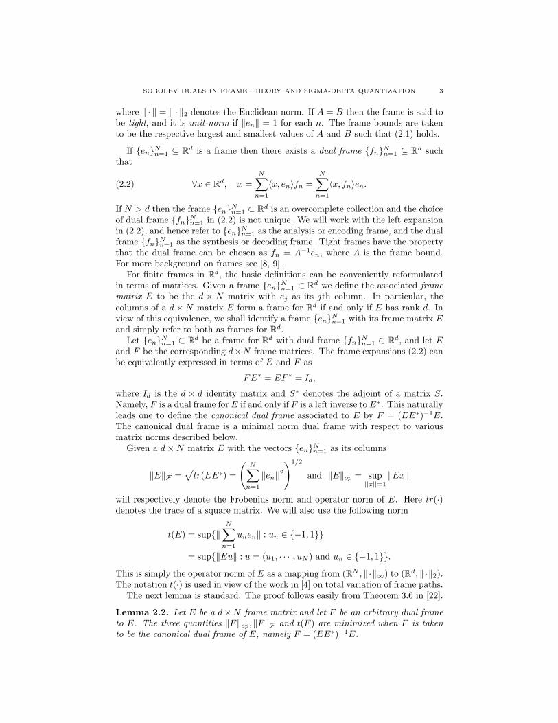
Example 5.2. Roots-of-unity frame path. Consider the frame path defined byE(t) = [cos(2πt), sin(2πt)]∗. It is well known, e.g., [13], that for each N ≥ 3, thecollection UN = {E(n/N)}Nn=1 ⊂ R2 given by

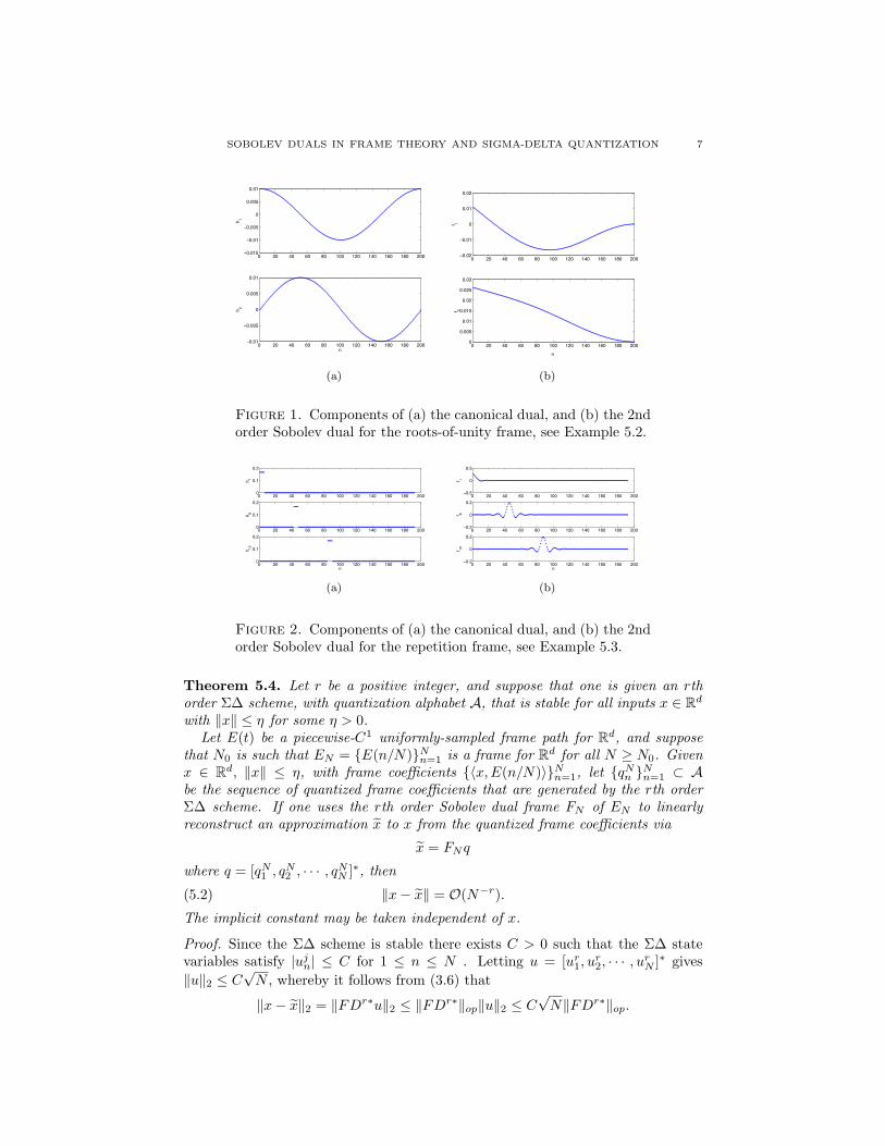
(5.1) E(n/N) = [cos(2πn/N), sin(2πn/N)]∗, 1 ≤ n ≤ N,is a unit-norm tight frame for R2. Figure 1 shows coordinate components of (a) thecanonical dual of U200 for R2, and (b) the associated 2nd order Sobolev dual.

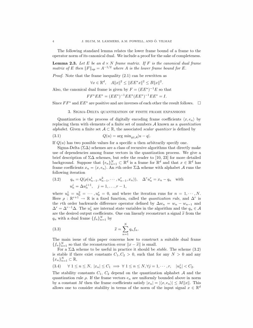
Example 5.3. Repetition frame path. Consider the frame path

E(t) = [χ[0, 1d ](t), χ( 1d ,

2d ](t), · · ·χ( d−1

d ,1](t)]∗,

where χS denotes the characteristic function of S. Note that RN = {E(n/N)}Nn=1

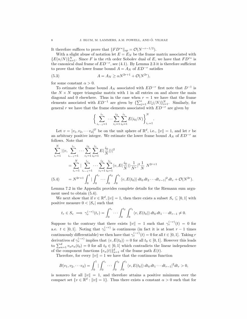
is a frame for Rd for all N ≥ d. When N ∈ dN, then RN is obtained by N -foldrepetition of the standard basis for Rd, hence the name repetition frame. For d = 32and N = 192, Figure 2 shows (a) the components h1, h8, and h15 of the canonicaldual of the repetition frame R192 in R32, and (b) the components f1, f8, and f15of the associated 2nd order Sobolev dual.

For s ∈ R, we say that f(N) = O(Ns) if lim supN→∞N−s|f(N)| <∞.


0 20 40 60 80 100 120 140 160 180 200−0.015

−0.01

−0.005

0

0.005

0.01

h 1

0 20 40 60 80 100 120 140 160 180 200−0.01

−0.005

0

0.005

0.01

n

h 2

(a)

0 20 40 60 80 100 120 140 160 180 200−0.02

−0.01

0

0.01

0.02

f 1

0 20 40 60 80 100 120 140 160 180 2000

0.005

0.01

0.015

0.02

0.025

0.03

n

f 2

(b)

Figure 1. Components of (a) the canonical dual, and (b) the 2ndorder Sobolev dual for the roots-of-unity frame, see Example 5.2.

0 20 40 60 80 100 120 140 160 180 2000

0.1

0.2

h 1

0 20 40 60 80 100 120 140 160 180 2000

0.1

0.2

h 8

0 20 40 60 80 100 120 140 160 180 2000

0.1

0.2

n

h 15

(a)

0 20 40 60 80 100 120 140 160 180 200−0.5

0

0.5

f 1

0 20 40 60 80 100 120 140 160 180 200−0.2

0

0.2

f 8

0 20 40 60 80 100 120 140 160 180 200−0.2

0

0.2

n

f 15

(b)

Figure 2. Components of (a) the canonical dual, and (b) the 2ndorder Sobolev dual for the repetition frame, see Example 5.3.

Theorem 5.4. Let r be a positive integer, and suppose that one is given an rthorder Σ∆ scheme, with quantization alphabet A, that is stable for all inputs x ∈ Rdwith ‖x‖ ≤ η for some η > 0.

Let E(t) be a piecewise-C1 uniformly-sampled frame path for Rd, and supposethat N0 is such that EN = {E(n/N)}Nn=1 is a frame for Rd for all N ≥ N0. Givenx ∈ Rd, ‖x‖ ≤ η, with frame coefficients {〈x,E(n/N)〉}Nn=1, let {qNn }Nn=1 ⊂ Abe the sequence of quantized frame coefficients that are generated by the rth orderΣ∆ scheme. If one uses the rth order Sobolev dual frame FN of EN to linearlyreconstruct an approximation x to x from the quantized frame coefficients via

x = FNq

where q = [qN1 , qN2 , · · · , qNN ]∗, then

(5.2) ‖x− x‖ = O(N−r).

The implicit constant may be taken independent of x.

Proof. Since the Σ∆ scheme is stable there exists C > 0 such that the Σ∆ statevariables satisfy |ujn| ≤ C for 1 ≤ n ≤ N . Letting u = [ur1, u

r2, · · · , urN ]∗ gives

‖u‖2 ≤ C√N, whereby it follows from (3.6) that

‖x− x‖2 = ‖FDr∗u‖2 ≤ ‖FDr∗‖op‖u‖2 ≤ C√N‖FDr∗‖op.


It therefore suffices to prove that ‖FDr∗‖op = O(N−r−1/2).With a slight abuse of notation let E = EN be the frame matrix associated with

{E(n/N)}Nn=1. Since F is the rth order Sobolev dual of E, we have that FDr∗ isthe canonical dual frame of ED−r, see (4.1). By Lemma 2.3 it is therefore sufficientto prove that the lower frame bound A = AN of ED−r satisfies

(5.3) A = AN ≥ αN2r+1 +O(N2r),

for some constant α > 0.To estimate the frame bound AN associated with ED−r first note that D−1 is

the N × N upper triangular matrix with 1 in all entries on and above the maindiagonal and 0 elsewhere. Thus in the case when r = 1 we have that the frameelements associated with ED−1 are given by {

∑ij=1E(j/N)}Ni=1. Similarly, for

general r we have that the frame elements associated with ED−r are given by{ ir∑ir−1=1

· · ·i2∑i1=1

i1∑i0=1

E(i0/N)}Nir=1

.

Let v = [v1, v2, · · · vd]T be on the unit sphere of Rd, i.e., ‖v‖ = 1, and let r bean arbitrary positive integer. We estimate the lower frame bound AN of ED−r asfollows. Note that

N∑ir=1

|〈v,ir∑

ir−1=1

· · ·i2∑i1=1

i1∑i0=1

E(i0N

)〉|2

=N∑ir=1

|ir∑

ir−1=1

· · ·i2∑i1=1

i1∑i0=1

〈v,E(i0N

)〉 1Nr|2 1N

N2r+1

= N2r+1

∫ 1

0

|∫ tr

0

· · ·∫ t2

0

∫ t1

0

〈v,E(t0)〉 dt0 dt2 · · · dtr−1|2 dtr +O(N2r).(5.4)

Lemma 7.2 in the Appendix provides complete details for the Riemann sum argu-ment used to obtain (5.4).

We next show that if v ∈ Rd, ‖v‖ = 1, then there exists a subset Sv ⊆ [0, 1] withpositive measure 0 < |Sv| such that

tr ∈ Sv =⇒ γ(−r)v (tr) =

∫ tr

0

· · ·∫ t2

0

∫ t1

0

〈v,E(t0)〉 dt0 dt1 · · · dtr−1 6= 0.

Suppose to the contrary that there exists ‖v‖ = 1 such that γ(−r)v (t) = 0 for

a.e. t ∈ [0, 1]. Noting that γ(−r)v is continuous (in fact it is at least r − 1 times

continuously differentiable) we then have that γ(−r)v (t) = 0 for all t ∈ [0, 1]. Taking r

derivatives of γ(−r)v implies that 〈v,E(t0)〉 = 0 for all t0 ∈ [0, 1]. However this leads

to∑dn=1 vnen(t0) = 0 for all t0 ∈ [0, 1] which contradicts the linear independence

of the component functions {en(t)}dn=1 of the frame path E(t).Therefore, for every ‖v‖ = 1 we have that the continuous function

B(v1, v2, · · · vd) =∫ 1

0

|∫ tr

0

· · ·∫ t2

0

∫ t1

0

〈v,E(t0)〉 dt0 dt1 · · · dtr−1|2dtr > 0,

is nonzero for all ‖v‖ = 1, and therefore attains a positive minimum over thecompact set {v ∈ Rd : ‖v‖ = 1}. Thus there exists a constant α > 0 such that for


all v ∈ Rd, ‖v‖ = 1,N∑ir=1

|〈v,ir∑

ir−1=1

· · ·i2∑i1=1

i1∑i0=1

E(i0N

)〉|2 ≥ αN2r+1 +O(N2r).

It follows that (5.3) holds. This completes the proof. �

Sobolev duals are hierarchical in the following sense: if quantization is performedwith an rth order Σ∆ scheme, and if the decoding party uses a Sobolev dual oforder s < r, then the approximation error will be of order O(N−s). This followsby using norm properties of the rth order Sobolev dual (see the proof of Theorem5.4) and ‖D‖op ≤ 2 to obtain

‖FDr∗‖op ≤ ‖FDs∗‖op‖D(r−s)∗‖op ≤ O(N−s−1/2) 2(r−s) = O(N−s−1/2),

which implies that the approximation error satisfies ‖x − x‖ = O(N−s). Thus,depending on the required precision, one can use a lower order Sobolev dual, andthereby reduce the computational resources required to construct the dual.

6. Mean Squared Error for Σ∆ quantization with Sobolev duals

This section shows that linear reconstruction with Sobolev duals achieves mini-mal mean squared error (MSE) under the Σ∆ white noise assumption (Σ∆-WNA).

Statistical noise models have a long history in the analysis and design of quantiza-tion algorithms, with the general goal being to replace or approximate deterministicanalysis with reasonable statistical models. Bennett’s classical work [3] modeled in-dividual coefficient quantization errors in simple scalar quantization as independentuniform random variables. While Bennett’s noise model has mathematical short-comings, it is known to be empirically accurate in many settings, especially whenthe quantizer step size is small, e.g., see [3, 20, 15]. Similar noise models have beenapplied to the analysis of Σ∆ algorithms, e.g., [15, 23, 24, 6, 2]. We shall considerthe following Σ∆ noise model that treats the Σ∆ state variables un in (3.6) asindependent identically distributed (i.i.d.) random variables.

Design Criterion 6.1 (Σ∆-WNA). Suppose that x, the vector to be quantized,is chosen randomly according to some probability measure supported on a compactset in Rd, and quantized with an rth-order Σ∆ scheme. Model the correspondingΣ∆ state variables {un}Nn=1 in (3.6) as independent, identically distributed randomvariables with mean zero and variance σ2.

We previously saw that the state variables for the first order Σ∆ scheme inExample 3.1 satisfy |un| ≤ δ/2. In view of this, it is common to model the statevariables un as uniform random variables on [−δ/2, δ/2]. Ergodic properties of thestate variables, e.g., see [17, 18], are also closely related to the uniform distribution.We emphasize that the Σ∆-WNA is not mathematically rigorous but is nonethelessempirically reasonable in many settings. For this reason, we simply view the noisemodel as a useful design criterion, and refer to [24, 14, 16, 15] for discussion of itsmathematical validity.

Theorem 6.2. Let {en}Nn=1 ⊂ Rd be a frame for Rd with frame matrix E. Supposethat x is randomly drawn from a compact set B in Rd according to a Borel probabilitymeasure p, supported on B, and suppose that the frame coefficients {〈x, en〉}Nn=1 are


102

10−5

10−4

10−3

10−2

10−1

100

N (number of elements in the frame)Third order scheme (repetition frame)

max

imum

erro

r (2−

norm

)

AltdualCandualC/Nc/N3

(a)

102

10−5

10−4

10−3

10−2

10−1

100

N (number of elements in the frame)Third order scheme (roots−of−unity frame)

max

imum

erro

r (2−

norm

)

AltdualCandualC/Nc/N3

(b)

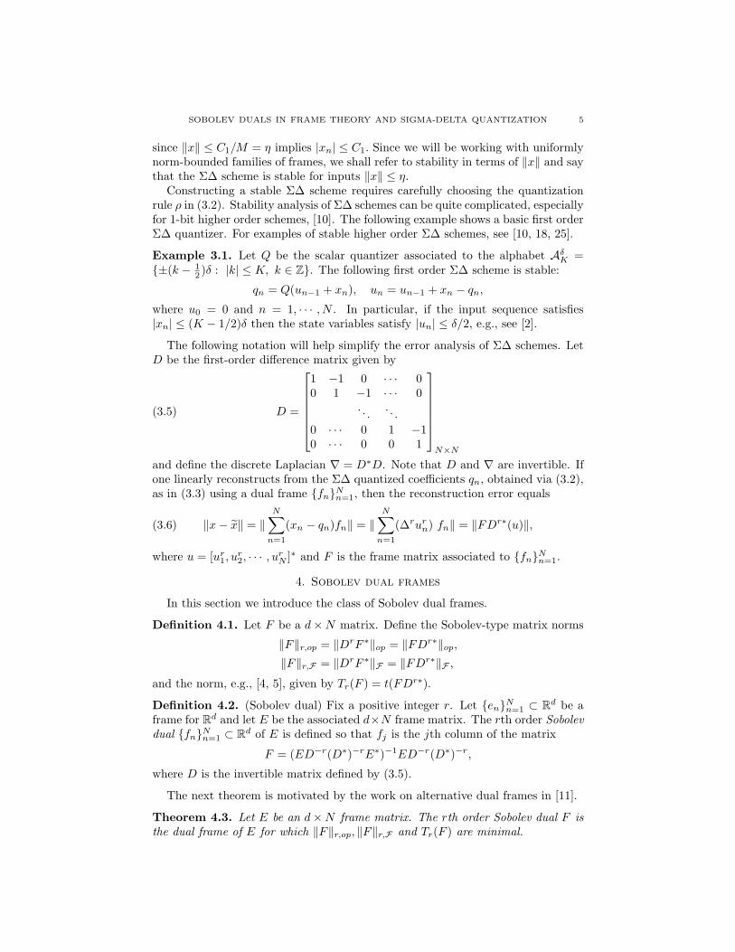
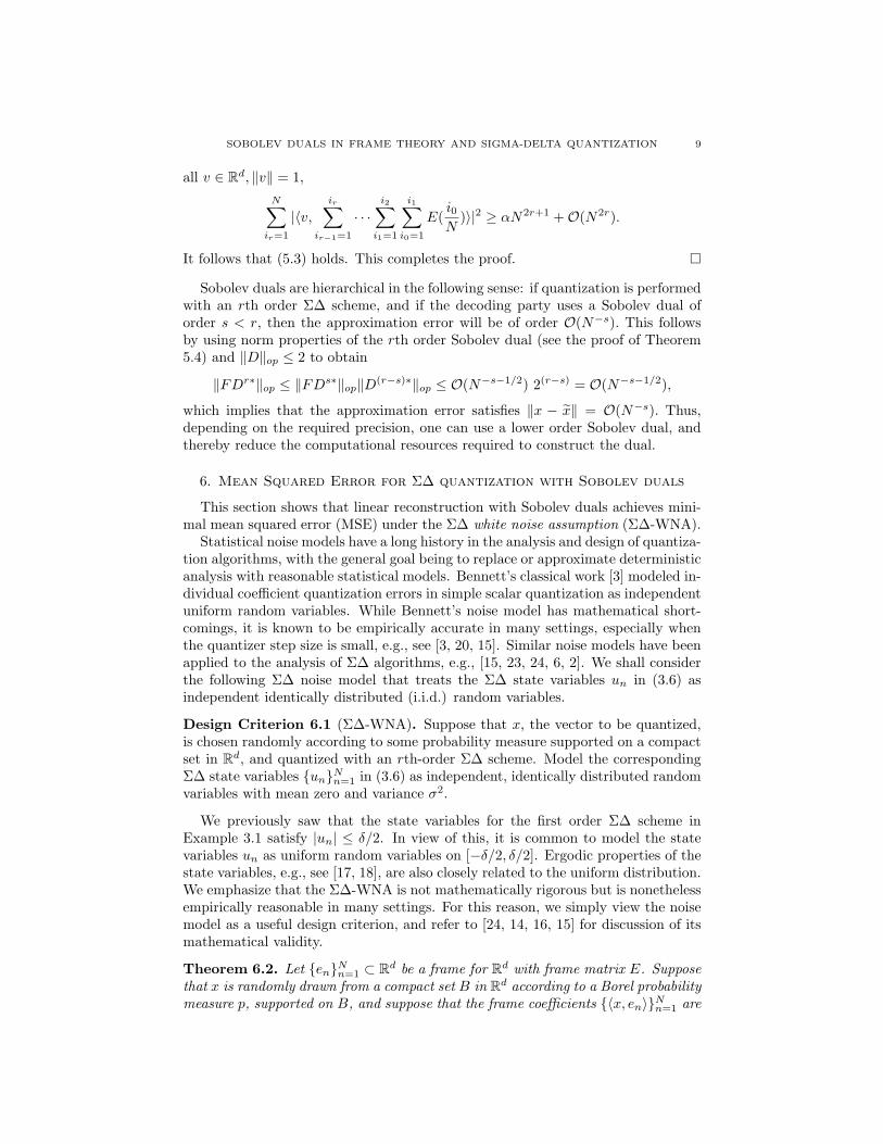
Figure 3. Comparison of worst case error in Σ∆ reconstructionwith canonical duals and Sobolev duals, see Example 7.1. Errorsfor (a) repetition frame path, and (b) roots-of-unity frame path.

quantized using an rth order Σ∆ scheme that is stable on B. Under the Σ∆-WNA,among all dual frames F of E, the rth-order Sobolev dual minimizes the MSE

MSE = E‖x− x‖2,

where x = xF is as in (3.3), and E denotes the expectation with respect to theprobability measure p.

Proof. Let E be a frame and let F be any dual frame. It follows from (3.6) thatthe MSE is given by

MSE = E‖x− x‖2 = E[〈FDr∗u, FDr∗u〉] = σ2‖FDr∗‖2F .

By Theorem 4.3 the MSE is minimal when F is the rth order Sobolev dual of E. �

7. Numerical example

The following experiment numerically compares the performance of Sobolev du-als and canonical dual frames for reconstructing Σ∆ quantized frame coefficients.

Example 7.1. 30 points in R2 are randomly chosen according to the uniformdistribution on the unit-square. For each of the 30 points, the corresponding framecoefficients with respect to the repetition frame RN are quantized using the 3rdorder Σ∆ scheme from [10]. Linear reconstruction is then performed with each ofthe 30 sets of quantized coefficients using both the canonical dual frame and the 3rdorder Sobolev dual of RN . Candual(N) and Altdual(N) will denote the largest ofthe 30 errors obtained using the canonical dual frame and Sobolev dual respectively.Part (a) in Figure 3 shows a log-log plot of Altdual(N) and Candual(N) againstthe frame size N . For comparison, log-log plots of 1/N3 and 1/N are also given.

Part (b) in Figure 3 repeats the above experiment using the roots-of-unity frameinstead of the repetition frame. In this case, note the split behavior in the canonicalreconstruction which was discussed in [21]. In both parts (a) and (b) Sobolev dualsyield smaller reconstruction error than canonical dual frames.


Appendix

In this section, we provide the details of the Riemann sum estimates that wereused in the proof of Theorem 5.4.

Lemma 7.2. Let r be a positive integer, E(t) a piecewise-C1 uniformly-sampledframe path for Rd, and suppose v is on the unit sphere of Rd. Denote

Sr =N∑ir=1

|〈v,ir∑

ir−1=1

· · ·i2∑i1=1

i1∑i0=1

E(i0N

)〉|2

Then

(7.1) Sr = N2r+1

∫ 1

0

|∫ tr

0

· · ·∫ t2

0

∫ t1

0

〈v,E(t0)〉 dt0 dt2 · · · dtr−1|2 dtr +O(N2r).

Proof. We first show that (7.1) holds when the frame path E is C1, i.e., the com-ponent functions are all continuously differentiable on [0, 1]. Our proof shall bein several steps. First, we introduce notation to simplify our task. Let γ(t) =〈v,E(t)〉 =

∑dn=1 vnen(t), and note that γ is continuously differentiable on [0, 1].

In parts (i) through (v) of the proof, ‖ · ‖L∞ denotes ‖ · ‖L∞[0,1]. For a positiveinteger k, γ(−k) shall denote the kth antiderivative of γ with dj/(dxj)[γ(−k)](0) = 0for all 0 ≤ j < k; we also define γ(0) = γ and γ(1) = γ′.

(i) Using the new notation, we have

Sr =N∑ir=1

|ir∑

ir−1=1

· · ·i2∑i1=1

i1∑i0=1

γ(i0/N)|2,

and the claim of the lemma can be rewritten as

Sr = N2r+1

∫ 1

0

|γ(−r)(t)|2dt+O(N2r).

(ii) For any function g that is continuously differentiable on [0, 1], and for anypositive integer M ≤ N , we have

(7.2) |Ng(−1)(M/N)−M∑m=1

g(m/N)| ≤ M

N‖g′‖L∞ .

This is a simple consequence of the mean value theorem.

(iii) We have

L(ir) :=ir∑

ir−1=1

· · ·i2∑i1=1

i1∑i0=1

γ(i0/N) = Nrγ(−r)(ir/N) +O(Nr−1).

To see this, note that by (7.2) we have

|Nγ(−1)(i1/N)−i1∑i0=1

γ(i0/N)| ≤ i1N‖γ′‖L∞ , and(7.3)

|N2γ(−2)(i2/N)−i2∑i1=1

Nγ(−1)(i1/N)| ≤ i2‖γ‖L∞ ,(7.4)


which imply

|N2γ(−2)(i2/N)−i2∑i1=1

i1∑i0=1

γ(i0/N)| ≤i2∑i1=1

i1N‖γ′‖L∞ + i2‖γ‖L∞

≤ i22N‖γ′‖L∞ + i2‖γ‖L∞ .(7.5)

By applying this argument repeatedly, it is easy to see that

|Nrγ(−r)(ir/N)− L(ir)| ≤r∑

m=1

imr Nr−m−1‖γ(m−r+1)‖L∞ ≤ CrNr−1

where we used the fact that 0 ≤ ir ≤ N . Here Cr is a constant that only dependson r and on E (recall that ‖v‖2 = 1, consequently ‖γ(m)‖L∞ ≤

∑dn=1 ‖e

(m)n ‖L∞ for

any integer m ≤ 1).

(iv) We next observe

|(Nrγ(−r)(ir/N))2 − |L(ir)|2| = |Nrγ(−r)(ir/N)− L(ir)||Nrγ(−r)(ir/N) + L(ir)|

≤ 2CrN2r−1‖γ(−r)‖L∞ + C2rN

2r−2

≤ N2r−1(2Cr‖γ(−r)‖L∞ + C2r/N)

≤ CrN2r−1(7.6)

where Cr = 2Cr‖γ(−r)‖L∞ + C2r . Consequently, we get

|N∑ir=1

N2r|γ(−r)(ir/N)|2 − Sr| = |N∑ir=1

N2r|γ(−r)(ir/N)|2 −N∑ir=1

|L(ir)|2|

≤N∑ir=1

CrN2r−1 = CrN

2r.

(v) We finally approximate∑Nir=1N

2r|γ(−r)(ir/N)|2 by an integral. In particular,

N∑ir=1

N2r|γ(−r)(ir/N)|2 = N2r+1N∑ir=1

|γ(−r)(ir/N)|2 1N︸︷︷︸

Ir

,

and, as Ir is a Riemann sum,

|Ir −∫ 1

0

|γ(−r)(t)|2dt| ≤ CrN

where Cr is the L∞-norm of the derivative of [γ(−r)]2. It follows

|N2r+1

∫ 1

0

|γ(−r)(t)|2dt− Sr| ≤ (Cr + Cr)N2r

which concludes the proof when the frame path is C1.(vi) For the extension of this result to the case when E is piecewise C1 one needsonly to modify (7.2), which changes the value of Cr. For simplicity, consider thecase g(x) = f(x)χ[0,a)(x) + h(x)χ[a,1](x), where 0 < a < 1, and f, h are C1 on theappropriate domains. Clearly, for M ∈ N such that M

N < a, (7.2) holds. For the


case MN ≥ a, we adjust the constant on the right-hand side of (7.2) as follows. Let

k ∈ N be so that kN ≤ a <

k+1N . Hence, (a− k

N ) < 1N . Thus

|N∫ M

N

0

g(t)dt−M∑m=1

g(m/N)|

= |N∫ a

0

f(t)dt−k∑

m=1

f(m/N) +N

∫ MN

a

h(t)dt−M∑

m=k+1

h(m/N)|

≤ |N∫ k/N

0

f(t)dt−k∑

m=1

f(m/N)|+ |N∫ a

k/N

f(t)dt|

+ |N∫ k+1

N

a

h(t)dt− h(k + 1N

) +N

∫ MN

k+1N

h(t)dt−M∑

m=k+2

h(m/N)|

≤ k

N‖f ′‖L∞[0,a) + ‖f‖L∞[0,a) + |N

∫ k+1N

a

h(t)dt− (k + 1− aN)h(k + 1N

)|

+ |(k − aN)h(k + 1N

)|+(M

N− k + 1

N

)‖h′‖L∞[a,1]

≤ M

N||f ′||L∞[0,a) +

M

Na||f ||L∞[0,a) + |k + 1− aN | 1

N‖h′‖L∞[a,1]

+ ‖h‖L∞[a,1] +(M

N− k + 1

N

)‖h′‖L∞[a,1]

≤ M

N||f ′||L∞[0,a) +

M

Na

(||f ||L∞[0,a) + ||h||L∞[a,1]

)+(M

N− a)‖h′‖L∞[a,1] ≤ K

M

N,

where K = ‖f ′‖L∞[0,a) + (2/a)‖g‖L∞[0,1] + ‖h′‖L∞[a,1]. So, on the right side of(7.2), we replace ‖g′‖L∞ with a constant K that depends only on the frame path.The remainder of the proof proceeds as in parts (iii) through (v), with the modifiedconstant K changing the constant on the right side of (7.3), and consequently Cr.This argument similarly extends to general functions g that are piecewise C1. �

Acknowledgments

The authors thank Radu Balan, Bernhard Bodmann, Sinan Gunturk, NguyenThao, and Yang Wang for valuable discussions related to the material. Portionsof this work were performed during visits at the Erwin Schrodinger Institute (ESI)in Vienna, and at a workshop at the Banff International Research Station (BIRS).M. Lammers, A. Powell, and O. Yılmaz gratefully acknowledge ESI and BIRS fortheir hospitality and support, and thank Hans Feichtinger for having helped arrangetheir visits to ESI. Final portions of this work were completed while A. Powell wasa visitor at the Academia Sinica, Institute for Mathematics in Taipei, Taiwan. Thisauthor gratefully acknowledges the Academia Sinica for its hospitality and support.

References

1. J.J. Benedetto, A.M. Powell, and O. Yılmaz, Second order sigma–delta (Σ∆) quantization offinite frame expansions, Appl. Comput. Harmon. Anal 20 (2006), 126–148.

2. , Sigma-delta (Σ∆) quantization and finite frames, IEEE Transactions on InformationTheory 52 (2006), no. 5, 1990–2005.

3. W.R. Bennett, Spectra of quantized signals, Bell Syst. Tech. J 27 (1948), no. 3, 446–472.


4. B.G. Bodmann and V.I. Paulsen, Frame paths and error bounds for sigma–delta quantization,

Applied and Computational Harmonic Analysis 22 (2007), no. 2, 176–197.

5. B.G. Bodmann, V.I. Paulsen, and S.A. Abdulbaki, Smooth Frame-Path Termination forHigher Order Sigma-Delta Quantization, Journal of Fourier Analysis and Applications 13

(2007), no. 3, 285–307.

6. H. Bolcskei and F. Hlawatsch, Noise reduction in oversampled filter banks using predictivequantization, IEEE Transactions on Information Theory 47 (2001), no. 1, 155–172.

7. P.T. Boufounos and A.V. Oppenheim, Quantization Noise Shaping on Arbitrary Frame Ex-

pansions, EURASIP Journal on Applied Signal Processing 2006, Article ID 53807.8. P.G. Casazza, The art of frame theory, Taiwanese J. Math 4 (2000), no. 2, 129–201.

9. O. Christensen, An Introduction to Frames and Riesz Bases, Birkhauser, 2003.

10. I. Daubechies and R. DeVore, Approximating a bandlimited function using very coarsely quan-tized data: A family of stable sigma-delta modulators of arbitrary order, Annals of Mathe-

matics 158 (2003), no. 2, 679–710.11. I. Daubechies, H.J. Landau, and Z. Landau, Gabor Time-Frequency Lattices and the Wexler-

Raz Identity, Journal of Fourier Analysis and Applications 1 (1994), no. 4, 437–478.

12. V.K. Goyal, J. Kovacevic, and J.A. Kelner, Quantized Frame Expansions with Erasures,Applied and Computational Harmonic Analysis 10 (2001), no. 3, 203–233.

13. V.K. Goyal, M. Vetterli, and N.T. Thao, Quantized overcomplete expansions in RN : analysis,

synthesis, and algorithms, IEEE Transactions on Information Theory 44 (1998), no. 1, 16–31.14. R.M. Gray, Spectral analysis of quantization noise in a single-loop sigma-delta modulator with

DC input, IEEE Transactions on Communications 37 (1989), no. 6, 588–599.

15. , Quantization noise spectra, IEEE Transactions on Information Theory 36 (1990),no. 6, 1220–1244.

16. R.M. Gray, W. Chou, and P.W. Wong, Quantization noise in single-loop sigma-delta modula-tion with sinusoidal inputs, IEEE Transactions on Communications 37 (1989), no. 9, 956–968.

17. C.S. Gunturk, Approximating a bandlimited function using very coarsely quantized data: im-

proved error estimates in sigma-delta modulation, Journal of the American MathematicalSociety 17 (2004), no. 1, 229–242.

18. C.S. Gunturk and N.T. Thao, Ergodic dynamics in sigma-delta quantization: tiling invariant

sets and spectral analysis of error, Adv. in Appl. Math. 34 (2005), no. 3, 523–560.19. H. Inose and Y. Yasuda, A unity bit coding method by negative feedback, Proceedings of the

IEEE 51 (1963), no. 11, 1524–1535.

20. D. Jimenez, L. Wang, and Y. Wang, White noise hypothesis for uniform quantization errors,SIAM Journal on Mathematical Analysis 38 (2007), 2042–2056.

21. M. Lammers, A.M. Powell, and O. Yılmaz, Alternative dual frames for digital-to-analog con-version in Sigma-Delta quantization, Advances in Computational Mathematics (2008), To

appear.

22. S. Li, On general frame decompositions, Numerical Functional Analysis and Optimization 16(1995), no. 9, 1181–1191.

23. R. Schreier and G.C. Temes, Understanding delta-sigma data converters, John Wiley & Sons,

2004.24. Y. Wang, Sigma-delta quantization errors and the traveling salesman problem, Adv. Comput.

Math. 28 (2008), no. 2, 101–118.

25. O. Yılmaz, Stability analysis for several second-order sigma-delta methods of coarse quanti-

zation of bandlimited functions, Constructive approximation 18 (2002), no. 4, 599–623.

Department of Mathematics, University of North Carolina at Wilmington, Wilm-

ington, NC 28403, USAE-mail address: [email protected]

E-mail address: [email protected]

Vanderbilt University, Department of Mathematics, Nashville, TN 37240, USA

E-mail address: [email protected]

Department of Mathematics, University of British Columbia, Vancouver, B.C. Canada

V6T 1Z2E-mail address: [email protected]

SOBOLEV DUALS IN FRAME THEORY AND SIGMA-DELTA …

Documents

Transcript of SOBOLEV DUALS IN FRAME THEORY AND SIGMA-DELTA …