Sobolev Duals for Random Frames and

Σ∆ Quantization of Compressed Sensing Measurements

C.S. Gunturk∗, M. Lammers†, A.M. Powell‡, R. Saab§, O. Yılmaz¶

October 10, 2012

Abstract

Quantization of compressed sensing measurements is typically justified by the robust recoveryresults of Candes, Romberg and Tao, and of Donoho. These results guarantee that if a uniformquantizer of step size δ is used to quantize m measurements y = Φx of a k-sparse signal x ∈ R

N ,where Φ satisfies the restricted isometry property, then the approximate recovery x# via ℓ1-minimization is within O(δ) of x. The simplest and commonly assumed approach is to quantizeeach measurement independently. In this paper, we show that if instead an rth order Σ∆ (Sigma-Delta) quantization scheme with the same output alphabet is used to quantize y, then there is analternative recovery method via Sobolev dual frames which guarantees a reduced approximationerror that is of the order δ(k/m)(r−1/2)α for any 0 < α < 1, if m &r,α k(logN)1/(1−α). Theresult holds with high probability on the initial draw of the measurement matrix Φ from theGaussian distribution, and uniformly for all k-sparse signals x whose magnitudes are suitablybounded away from zero on their support.

1 Introduction

Compressed sensing is concerned with when and how sparse signals can be recovered exactly orapproximately from few linear measurements [9, 11, 15]. Let Φ be an m×N matrix providing themeasurements where m ≪ N , and let ΣN

k denote the space of k-sparse signals in RN , k < m. A

standard objective, after a suitable change of basis, is that the mapping x 7→ y = Φx be injective onΣNk . Minimal conditions on Φ that offer such a guarantee are well-known (see, e.g. [12]) and require

at least that m ≥ 2k. On the other hand, under stricter conditions on Φ, such as the restrictedisometry property (RIP), one can recover sparse vectors from their measurements by numericallyefficient methods, such as ℓ1-minimization. Moreover, the recovery will also be robust when themeasurements are corrupted or perturbed [10], cf. [16]; if y = Φx + e where e is any vector suchthat ‖e‖2 ≤ ǫ, then the solution x# of the optimization problem

min ‖z‖1 subject to ‖Φz − y‖2 ≤ ǫ (1)

Communicated by Emmanuel Candes.

2010 Mathematics Subject Classification. 41A46, 94A12Key words and phrases. Quantization, finite frames, random frames, alternative duals, compressed sensing.

∗Courant Institute of Mathematical Sciences, New York University.†University of North Carolina, Wilmington.‡Vanderbilt University.§Duke University.¶University of British Columbia.

1

will satisfy ‖x− x#‖2 ≤ C1ǫ for some constant C1 = C1(Φ).The price paid for these stronger recovery guarantees is the somewhat smaller range of values

available for the dimensional parametersm, k, and N . While there are some explicit (deterministic)constructions of measurement matrices with stable recovery guarantees, best results (widest rangeof values) have been found via random families of matrices. For example, if the entries of Φ areindependently sampled from the Gaussian distribution N (0, 1

m), then with high probability, Φ willsatisfy the RIP (with a suitable set of parameters) if m ∼ k log(Nk ). Significant effort has been puton understanding the phase transition behavior of the RIP parameters for other random families,e.g., Bernoulli matrices and random Fourier samplers.

Main goal

To be amenable to digital processing and storage, applications require a quantization step wherethe measurements y are discretized in amplitude to become representable with a finite number ofbits. In this context, the robust recovery result mentioned above is essential to the practicabilityof compressed sensing and has been employed as the primary tool for the design and analysis ofquantization methods. The main goal of this paper is to develop and analyze the class of Σ∆algorithms as a high accuracy alternative for quantizing compressed sensing measurements. Inparticular, we propose and analyze a two-stage algorithm for reconstructing signals from theirΣ∆-quantized compressed sensing measurements. In the first stage, any standard reconstructionalgorithm for compressed sensing is used to recover the support T of the underlying sparse vector.In the second stage the vector itself is reconstructed using non-standard (Sobolev) duals of theassociated submatrix ΦT . Our main results, Theorem A and Theorem B, show that Σ∆ algorithmscan be used to provide high accuracy quantized representations in the settings of Gaussian randomfinite frames and compressed sensing measurements with Gaussian measurement matrices. Animportant theme in the main results is that Σ∆ algorithms yield quantization error bounds thatbecome quantifiably small as the ratio λ := m/k increases.

Quantization for compressed sensing measurements

Suppose a discrete alphabet A, such as A = δZ for some step size δ > 0, is to be employed to replaceeach measurement yj with a quantized measurement qj := yj ∈ A. In light of the robust recoveryresult mentioned above, the temptation would be to minimize ‖e‖2 = ‖y − q‖2 over q ∈ Am. Thisimmediately reduces to minimizing |yj−qj| for each j, i.e., quantizing each measurement separatelyto the nearest element of A, which is called memoryless scalar quantization (MSQ), also known aspulse code modulation (PCM).

Since ‖y − q‖2 ≤ 12δ√m, the robust recovery result guarantees that

‖x− x#MSQ‖2 . δ√m. (2)

Note that (2) is somewhat surprising as the reconstruction error bound does not improve by in-creasing the number of (quantized) measurements; on the contrary, it deteriorates. However, the√m term is an artifact of our choice of normalization for the measurement matrix Φ. In the com-

pressed sensing literature, it is conventional to normalize a (random) measurement matrix Φ sothat it has unit-norm columns (in expectation). This is the necessary scaling to achieve isome-try, and for random matrices it ensures that E‖Φx‖2 = ‖x‖2 for any x, which then leads to theRIP through concentration of measure and finally to the robust recovery result stated in (1). On

2

the other hand, this normalization imposes an m-dependent dynamic range for the measurementswhich scales as 1/

√m, hence it is not fair to use the same value δ for the quantizer resolution as

m increases. In this paper, we investigate the dependence of the recovery error on the number ofquantized measurements where δ is independent of m. A fair assessment of this dependence can bemade only if the dynamic range of each measurement is kept constant while increasing the numberof measurements. This suggests that the natural normalization in our setting should ensure thatthe entries of the measurement matrix Φ are independent of m. In the specific case of randommatrices, we can achieve this by choosing the entries of Φ standard i.i.d. random variables, e.g.according to N (0, 1). With this normalization of Φ, the robust recovery result of [10] stated at thebeginning now becomes

‖y − y‖2 ≤ ǫ =⇒ ‖x− x#‖2 ≤C1√mǫ, (3)

which also replaces (2) with

‖x− x#MSQ‖2 . δ. (4)

As expected, this error bound does not deteriorate with m anymore. In this paper, we will adoptthis normalization convention and work with the standard Gaussian distribution N (0, 1) whenquantization is involved, but also use the more typical normalization N (0, 1/m) for certain concen-tration estimates that will be derived in Section 3. The transition between these two conventionsis of course trivial.

The above analysis of quantization error is based on MSQ, which involves separate (indepen-dent) quantization of each measurement. The vast logarithmic reduction of the ambient dimensionN would seem to suggest that this strategy is essentially optimal since information appears to besqueezed (compressed) into few uncorrelated measurements. Perhaps for this reason, the existingliterature on quantization of compressed sensing measurements focused mainly on alternative recon-struction methods from MSQ-quantized measurements and variants thereof, e.g., [7,13,18,21,24,38].In addition to [8], which uses Σ∆ modulation to quantize x before the random measurements aremade, the only exceptions we are aware of are [29,33], where the authors model the sparse vectorsprobabilistically and construct non-uniform scalar quantizers that minimize the quantization erroramong all memoryless quantizers provided that the sparse vectors obey some probabilistic modeland that the recovery is done with the lasso formulation (see [34]) of (1).

On the other hand, it is clear that if (once) the support of the signal is known (recovered),then the m measurements that have been taken are highly redundant compared to the maximum kdegrees of freedom that the signal has on its support. At this point, the signal may be consideredoversampled. However, the error bound (4) does not offer an improvement of reconstruction accu-racy, even if additional samples become available. (The RIP parameters of Φ are likely to improveas m increases, but this does not seem to reflect on the implicit constant factor in (4) satisfactorily.)This is contrary to the conventional wisdom in the theory and practice of oversampled quantizationin A/D conversion where reconstruction error decreases as the sampling rate increases, especiallywith the use of quantization algorithms specially geared for the reconstruction procedure. The maingoal of this paper is to show how this can be done in the compressed sensing setting as well. Thetechnical results used to accomplish this main goal may be of independent mathematical interestas they establish lower bounds on the smallest singular values of random matrix products neededto control the operator norm of Sobolev duals of Gaussian random matrices.

3

Quantization for oversampled data

Methods of quantization have long been studied for oversampled data conversion. Sigma-delta(Σ∆) quantization (modulation), for instance, is the dominant method of A/D conversion foraudio signals and relies heavily on oversampling, see [14, 20, 28]. In this setting, oversampling istypically exploited to employ very coarse quantization (e.g., 1 bit/sample), however, the workingprinciple of Σ∆ quantization is applicable to any quantization alphabet. In fact, it is more naturalto consider Σ∆ quantization as a “noisea shaping” method, for it seeks a quantized signal (qj) bya recursive procedure to push the quantization error signal y− q towards an unoccupied portion ofthe signal spectrum. In the case of bandlimited signals, this would correspond to high frequencybands.

As the canonical example, the standard first-order Σ∆ quantizer with input (yj) computes abounded solution (uj) to the difference equation

(∆u)j := uj − uj−1 = yj − qj . (5)

This can be achieved recursively by choosing, for example,

qj = argminp∈A

|uj−1 + yj − p|. (6)

Since the reconstruction of oversampled bandlimited signals can be achieved with a low-pass filterϕ that can also be arranged to be well-localized in time, the reconstruction error ϕ∗(y−q) = ∆ϕ∗ubecomes small due to the smoothness of ϕ. It turns out that, with this procedure, the reconstructionerror is reduced by a factor of the oversampling ratio λ, defined to be the ratio of the actual samplingrate to the bandwidth of ϕ.

This principle can be iterated to set up higher-order Σ∆ quantization schemes. It is well-knownthat a reconstruction accuracy of order O(λ−r) can be achieved (in the supremum norm) if abounded solution to the equation ∆ru = y − q can be found [14] (here, r ∈ N is the order of theassociated Σ∆ scheme). The boundedness of u is important for practical implementation, but it isalso important for the error bound. The implicit constant in this bound depends on r as well as‖u‖∞. Fine analyses of carefully designed schemes have shown that optimizing the order can evenyield exponential accuracy O(e−cλ) for fixed sized finite alphabets A (see [20]), which is optimalb

apart from the value of the constant c.The above formulation of noise-shaping for oversampled data conversion generalizes naturally

to the problem of quantization of arbitrary frame expansions, e.g., [3]. Specifically, we will considerfinite frames in R

k. A collection (ej)mj=1 in R

k is a frame for Rk with frame bounds 0 < A ≤ B <∞if

∀x ∈ Rk, A‖x‖22 ≤

m∑

j=1

|〈x, ej〉|2 ≤ B‖x‖22.

aThe quantization error is often modeled as white noise in signal processing, hence the terminology. However ourtreatment of quantization error in this paper is entirely deterministic.

bThe optimality remark does not apply to the case of infinite quantization alphabet A = δZ because dependingon the coding algorithm, the (effective) bit-rate can still be unbounded. Indeed, arbitrarily small reconstruction errorcan be achieved with a (sufficiently large) fixed value of λ and a fixed value of δ by increasing the order r of the Σ∆modulator. This would not work with a finite alphabet because the modulator will eventually become unstable. Inpractice, almost all schemes need to use some form of finite quantization alphabet.

4

Suppose that we are given an input signal x and an analysis frame (ei)m1 of size m in R

k. We canrepresent the frame vectors as the rows of a full-rank m× k matrix E, the sampling operator. Theinput sequence y to be quantized will simply be the frame coefficients, i.e., y = Ex. Similarly, letus consider a corresponding synthesis frame (fj)

m1 . We stack these frame vectors along the columns

of a k×m matrix F , the reconstruction operator, which is then a left inverse of E, i.e., FE = I. Aquantization algorithm will replace the coefficient sequence y with its quantization q ∈ Am, whichwill then yield an approximate reconstruction x using the synthesis frame via x = Fq. Typically(y −Am) ∩Ker(F ) = ∅, so we have x 6= x. The reconstruction error is given by

x− x = F (y − q), (7)

and the goal of noise shaping amounts to arranging q in such a way that y − q is close to Ker(F ).If the sequence (fj)

m1 of dual frame vectors were known to vary smoothly in j (including smooth

termination into null vector), then Σ∆ quantization could be employed without much alteration,e.g., [6, 22]. However, this need not be the case for many examples of frames (together with theircanonical duals) that are used in practice. For this reason, it has recently been proposed in [5, 23]to use special alternative dual frames, called Sobolev dual frames, that are naturally adapted toΣ∆ quantization. It is shown in [5] (see also Section 2) that for any frame E, if a standard rthorder Σ∆ quantization algorithm with alphabet A = δZ is used to compute q := qΣ∆, then withan rth order Sobolev dual frame F := FSob,r and xΣ∆ := FSob,rqΣ∆, the reconstruction error obeysthe bound

‖x− xΣ∆‖2 .rδ√m

σmin(D−rE), (8)

where D is the m×m difference matrix defined by

Dij :=

1, if i = j,−1, if i = j + 1,0, otherwise,

(9)

and σmin(D−rE) stands for the smallest singular value of D−rE.

Contributions

For the compressed sensing application that is the subject of this paper, E will simply be a sub-matrix of the measurement matrix Φ, hence it may have been found by sampling an i.i.d. randomvariable. Minimum singular values of random matrices with i.i.d. entries have been studied ex-tensively in the mathematical literature. For an m × k random matrix E with m ≥ k and withi.i.d. entries sampled from a sub-Gaussian distribution with zero mean and unit variance,c one has

σmin(E) &√m−

√k (10)

with high probability [31]. Note that in general D−rE would not have i.i.d. entries. A naive lowerbound for σmin(D

−rE) would be σmin(D−r)σmin(E). However (see Proposition 3.2), σmin(D

−r)satisfies

σmin(D−r) ≍r 1, (11)

cAs mentioned earlier, we do not normalize the measurement matrix Φ in the quantization setting.

5

and therefore this naive product bound yields no improvement on the reconstruction error for Σ∆-quantized measurements over the bound (4) for MSQ-quantized ones. In fact, the true behavior ofσmin(D

−rE) turns out to be drastically different and is described in Theorem A, one of our mainresults (see also Theorem 3.8).

For simplicity, we shall work with standard i.i.d. Gaussian variables for the entries of E. Inanalogy with our earlier notation, we define the “oversampling ratio” λ of the frame E by

λ :=m

k. (12)

Theorem A. Let E be an m×k random matrix whose entries are i.i.d. N (0, 1). Given r ∈ N andα ∈ (0, 1), there exist constants c = c(r) > 0 and c′ = c′(r) > 0 such that if λ ≥ (c logm)1/(1−α),then with probability at least 1− exp(−c′mλ−α),

σmin(D−rE) &r λ

α(r− 1

2)√m, (13)

which yields the reconstruction error bound

‖x− xΣ∆‖2 .rδ√m

σmin(D−rE).r λ

−α(r− 1

2)δ. (14)

While the kind of decay in this error bound is familiar to Σ∆ modulation, the domain ofapplicability of this result is rather surprising. Previously, the only setting in which this type ofapproximation accuracy could be achieved (with or without Sobolev duals) was the case of highlystructured frames, e.g., when the frame vectors are found by sampling along a piecewise smoothframe path. Theorem A shows that such an accuracy is obtained even when the analysis frame isa random Gaussian matrix, provided the reconstruction is done via Sobolev duals.

It is worth commenting on how the error bound (14) relates to earlier work on Σ∆ quantizationof finite frames. To recast the current work in terms of frame theory, let ej ∈ R

k be the jth row ofthe measurement matrix E and let (ej)

mj=1 ⊂ R

k be the (analysis) frame associated to E. Previouswork in [5, 6, 22] for structured deterministic families of frames shows error bounds for rth orderΣ∆ quantization of the form Cr,k,δm

−r. The error bound (14) for random frames, rewritten as

‖x− xΣ∆‖2 .r,k,δ m−α(r− 1

2),

is not as strong as the deterministic m−r bound. This reduction in the error decay rate illus-trates the technical challenges and potential limitations that arise when one moves from structureddeterministic frames to unstructured random frames.

The manner in which frame vectors are normalized can affect how one interprets error boundssuch as (14). Theorem A uses an m× k i.i.d. N (0, 1) random matrix E and thus normalizes framevectors as E‖ej‖2 = k. Earlier work in [2, 3, 22] often prefers unit-norm frames, whereas the workin [5,6] imposes no explicit frame normalization but uses families of frames generated by a commonframe path. All of these cases involve frame vector normalizations that are essentially independentof the frame size m, and the dependence of error rates on m thus has a similar interpretation ineach approach.

In the compressed sensing setting, one needs (13) to be uniform for all the frames E that arefound by selecting k columns of Φ at a time. The proof of Theorem A extends in a straightforwardmanner to allow for this using a standard “union bound” argument, provided λ is known to be

6

slightly larger. More precisely, if Φ is an m×N matrix whose entries are i.i.d. according to N (0, 1),and if λ := m/k ≥ c(logN)1/(1−α), then (13) holds for all E = ΦT with #T ≤ k with the same typeof probability bound (with new constants). This result can be utilized to improve the reconstructionaccuracy of a sparse signal x from its Σ∆-quantized compressed sensing measurements if the supportT of x is known. This is because if T is known, ΦT is known, and its Sobolev dual can be found andused in the reconstruction. On the other hand, for most signals, recovering the exact or approximatesupport is already nearly guaranteed by the robust recovery result shown in (3) together with thestability of the associated Σ∆ quantizer. For example, a simple sufficient condition for full recoveryof the support is that all the |xj | for j ∈ T be larger than C‖y − qΣ∆‖2 for a suitable constant C.A precise version of this condition is stated in Theorem B.

In light of all these results, we propose Σ∆ quantization as a more effective alternative ofMSQ (independent quantization) for compressed sensing. Our approach assumes that (a boundfor) the sparsity level k is known – for perspective, several compressed sensing algorithms such asCoSaMP [26] and ROMP [27] also require knowledge of the sparsity level. With high probabilityon the measurement matrix, a significant improvement of the reconstruction accuracy of sparsesignals can be achieved through a two-stage recovery procedure:

1. Coarse recovery: ℓ1-minimization (or any other robust recovery procedure) applied to qΣ∆

yields an initial, “coarse” approximation x# of x, and in particular, the exact (or approximate)support T of x.

2. Fine recovery: Sobolev dual of the frame ΦT applied to qΣ∆ yields a finer approximationxΣ∆ of x.

Combining all these, our second main theorem follows (also see Theorem 4.2):

Theorem B. Let Φ be an m × N matrix whose entries are i.i.d. according to N (0, 1). Supposer ∈ N, α ∈ (0, 1) and λ := m/k ≥ c(logN)1/(1−α) where c = c(r, α) is an appropriate constant.Then there are two constants c′ and C that depend only on r such that with probability at least 1−exp(−c′mλ−α) on the draw of Φ, the following holds: For every x ∈ ΣN

k such that minj∈supp(x) |xj | ≥Cδ, the reconstruction xΣ∆ satisfies

‖x− xΣ∆‖2 .rδ√m

σmin(D−rE).r λ

−α(r− 1

2)δ. (15)

To put this result in perspective, note that the approximation error given in (15) decays asthe “redundancy” λ = m

k increases. In fact, by using an arbitrarily high order Σ∆ scheme, wecan make this decay faster than any power law (albeit with higher constants). Note that such adecay is not observed in the reconstruction error bound for MSQ given in (4). Of course, one couldargue that these upper bounds may not reflect the actual behavior of the error. However, in thesetting of frame quantization the performance of MSQ is well investigated. In particular, let E bean m× k real matrix, and let K be a bounded set in R

k. For x ∈ K, suppose we obtain qMSQ(x)by quantizing the entries of y = Ex using MSQ with alphabet A = δZ. Let ∆opt be an optimaldecoder. Then, Goyal et al. show in [19] that

[E ‖x−∆opt(qMSQ(x))‖22

]1/2&k λ

−1δ

7

where λ = m/k and the expectation is with respect a probability measure on x that is, for example,absolutely continuous. This lower bound limits the extent to which one can improve the reconstruc-tion by means of alternative reconstruction algorithms from MSQ-quantized compressed sensingmeasurements. On the other hand, setting, for example, α = 3/4 in Theorem B we observe thatif we use a second-order Σ∆ scheme to quantize the measurements, and if we adopt the two-stagerecovery procedure proposed above, the resulting approximation will be superior to that producedoptimally from MSQ-quantized measurements, provided λ = m/k is sufficiently large. Redundancyis built into the compressed sensing paradigm (we need λ & logN for the robust recovery result tohold), so this strategy is not contrary to the philosophy of compressed sensing and we might as wellutilize this redundancy when designing effective quantizers in this setup. Note that Theorem Brequires slightly more oversampling (λ & (logN)1/1−α) beyond what is common in compressedsensing – it is not clear if this is a consequence of our method of proof or if this extra oversamplingis theoretically necessary. Similarly, the λ-dependence in the probability of failure is also due to ourmethod of proof and may or may not be theoretically necessary. By rewriting the failure probabilityexp(−c′mλ−α) as exp(−c′m1−αkα), we observe that it is still possible to bound this probability byonly increasing the number of measurements m.

It is possible to imagine more sophisticated and more effective quantization and recovery algo-rithms for compressed sensing. However using Σ∆ quantization has a number of appealing features:

• It produces more accurate approximations than any known quantization scheme in thissetting (even when sophisticated recovery algorithms are employed).

• It is modular in the sense that if the fine recovery stage is not available or practical toimplement, then the standard (coarse) recovery procedure can still be applied as is.

• It is progressive in the sense that if new measurements arrive (in any given order), noiseshaping can be continued on these measurements as long as the state of the system (r realvalues for an rth order scheme) has been stored.

• It is universal in the sense that it uses no information about the measurement matrix or thesignal.

The paper is organized as follows. We review the basics of Σ∆ quantization and Sobolev duals inframe theory in Section 2, followed by the reconstruction error bounds for random Gaussian framesin Section 3. We then present the specifics of our proposed quantization and recovery algorithm forcompressed sensing in Section 4. We present our numerical experiments in Section 5 and concludewith extensions to more general settings in Section 6.

2 Background on Σ∆ quantization of frame expansions

Σ∆ quantization

The governing equation of a standard rth order Σ∆ quantization scheme with input y = (yj) andoutput q = (qj) is

(∆ru)j = yj − qj, j = 1, 2, . . . , (16)

8

where the qj ∈ A are chosen according to some quantization rule, typically a predetermined functionof the input and past state variables (ul)l<j , given by

qj = Q(uj−1, . . . , uj−T , yj, . . . , yj−S). (17)

Not all Σ∆ quantization schemes are presented (or implemented) in this canonical form, but theyall can be rewritten as such for an appropriate choice of r and u. We shall not be concerned withthe specifics of the mapping Q, except that it needs to be so that u is bounded. The smaller the sizeof the alphabet A gets relative to r, the harder it is to guarantee this property. The extreme caseis 1-bit quantization, i.e., |A| = 2, which is typically the most challenging setting. We will not beworking in this case. In fact, for our purposes, A will in general have to be sufficiently fine to allowfor the recovery of the support of sparse signals. In order to avoid technical difficulties, we shallwork with the infinite alphabet A = δZ, but also note that only a finite portion of this alphabet willbe used for bounded signals. A standard quantization rule that has this “boundedness” propertyis given by the greedy rule which minimizes |uj | given uj−1, . . . , uj−r and yj, i.e.,

qj = argmina∈A

∣∣∣r∑

i=1

(−1)i−1

(r

i

)uj−i + yj − a

∣∣∣. (18)

It is easy to check that with this rule, one has |uj | ≤ 2−1δ and |yj − qj| ≤ 2r−1δ. In turn, if‖y‖∞ < C, then one needs only L := 2⌈Cδ ⌉+ 2r + 1 levels. In this case, the associated quantizer issaid to be log2 L-bit, and we have

‖u‖∞ . δ and ‖y − q‖∞ .r δ. (19)

With more stringent quantization rules, the first inequality would also have an r-dependent con-stant. In fact, it is known that for quantization rules with a 1-bit alphabet, this constant will beas large as O(rr), e.g., see [14,20]. In this paper, unless otherwise stated, we shall be working withthe greedy quantization rule of (18).

The initial conditions of the recursion in (16) can be set arbitrarily, however for the purposesof this paper it will be convenient to set them equal to zero. With u−r+1 = · · · = u0 = 0, andj = 1, . . . ,m, the difference equation (16) can be rewritten as a matrix equation

Dru = y − q, (20)

where D is as in (9).As before, we assume E is an m × k matrix whose rows form the analysis frame and F is a

k ×m left inverse of E whose columns form the dual (synthesis) frame. Given any x ∈ Rk, we set

y = Ex, and denote its rth order Σ∆ quantization by qΣ∆ and its reconstruction by xΣ∆ := FqΣ∆.Substituting (20) into (7), we obtain the error expression

x− x = FDru. (21)

With this expression, ‖x− x‖ can be bounded for any norm ‖ · ‖ simply as

‖x− x‖ ≤ ‖u‖∞m∑

j=1

‖(FDr)j‖. (22)

9

Here (FDr)j is the jth column of FDr. This bound is also valid in infinite dimensions, and infact has been used extensively in the mathematical treatment of oversampled A/D conversion ofbandlimited functions.

For r = 1 and ‖ · ‖ = ‖ · ‖2, the sum term on the right hand side of (22) motivated the study ofthe so-called frame variation defined by

V (F ) :=m∑

j=1

‖fj − fj+1‖2, (23)

where (fj) are the columns of F , and one defines fm+1 = 0; see [3]. Higher-order frame variationsto be used with higher-order Σ∆ schemes are defined similarly; see [2]. Frames (analysis as well assynthesis) that are obtained via uniform sampling a smooth curve in R

k (so-called frame path) aretypical in many settings. However, the “frame variation bound” is useful in finite dimensions onlywhen the frame path terminates smoothly. Otherwise, it typically does not provide higher-orderreconstruction accuracy (see [2] for an exception). Designing smoothly terminating frames can betechnically challenging, e.g., [6].

Sobolev duals

Recently, a more straightforward approach was proposed in [22] for the design of (alternate) dualsof finite frames for Σ∆ quantization. Here, one instead considers the operator norm of FDr on ℓ2and the corresponding bound

‖x− x‖2 ≤ ‖FDr‖op‖u‖2. (24)

Note that this bound is not available in the infinite dimensional setting of bandlimited functionsdue to the fact that u is typically not in ℓ2. It is now natural to minimize ‖FDr‖op over all dualframes of a given analysis frame E. These frames, introduced in [5], have been called Sobolev duals,in analogy with ℓ2-type Sobolev (semi)norms.

Σ∆ quantization algorithms are normally designed for analog circuit operation, so they control‖u‖∞, which would control ‖u‖2 only in a suboptimal way. However, it turns out that there areimportant advantages in working with the ℓ2 norm in the analysis. The first advantage is thatSobolev duals are readily available by an explicit formula. The solution Fsob,r of the optimizationproblem

minF

‖FDr‖op subject to FE = I (25)

is given by the matrix equationFsob,rD

r = (D−rE)†, (26)

where † stands for the Moore-Penrose inversion operator, which, in our case, is given by E† :=(E∗E)−1E∗. Note that for r = 0 (i.e., no noise-shaping, or MSQ), one simply obtains F = E†, thecanonical dual frame of E.

The second advantage of this approach is its analytic tractability. Plugging (26) into (24), itimmediately follows that

‖x− x‖2 ≤ ‖(D−rE)†‖op‖u‖2 =1

σmin(D−rE)‖u‖2, (27)

where σmin(D−rE) stands for the smallest singular value of D−rE. There exist highly developed

methods for estimating spectral norms and more generally singular values of matrices, especiallyin the random setting, as we shall employ in this paper.

10

3 Reconstruction error bound for random frames

In what follows, σj(A) will denote the jth largest singular value of the matrix A. Similarly,λj(B) will denote the jth largest eigenvalue of the Hermitian matrix B. Hence, we have σj(A) =√λj(A∗A). We will also use the notation Σ(A) for the diagonal matrix of singular values of A,

with the convention (Σ(A))jj = σj(A). All matrices in our discussion will be real valued and theHermitian conjugate reduces to the transpose.

The remainder of this section is dedicated to proving the main results of the paper. Let E be anm×k matrix with i.i.d. entries drawn from N (0, 1/m). In Section 3.1, we show that if m/k is largeenough, σmin(D

−rE) & (m/k)α(r−1/2), with high probability (Theorem 3.8, equivalently TheoremA). To obtain this result, we use a property of Gaussian vectors (Proposition 3.3) and a standardǫ-net argument to upper bound the norm ‖SE‖ℓm

2→ℓk

2

with high probability for an arbitrary positive

diagonal matrix S (Lemma 3.4). Next, we again use properties of Gaussian vectors (Proposition3.5 and Corollary 3.6) and an ǫ-net argument to lower bound the least singular value of SE, withhigh probability, under mild conditions on S (Theorem 3.7). By a careful choice of parameters inthe above results and for S = Σ(D−r), we then obtain Theorem 3.8.

In Section 3.2, we generalize Theorem 3.8 to the compressed sensing setting. In particular,we use a standard union bound to show that if m/k is large enough, then with high probability,σmin(D

−rE) & (m/k)α(r−1/2), for any m× k sub-matrix E, of an m×N random matrix Φ whoseentries are drawn i.i.d. from N (0, 1/m) (Theorem 3.9).

3.1 Lower bound for σmin(D−rE)

We have seen that the main object of interest for the reconstruction error bound is σmin(D−rE) for

a random frame E. Since we focus on the case when E is a Gaussian random matrix, the followinglemma will be useful for obtaining bounds on singular values.

Lemma 3.1. Let H be an m × m square matrix. If E is an m × k matrix with i.i.d. N (0, σ2)entries then the distribution of Σ(HE) is the same as the distribution of Σ(Σ(H)E).

Proof. Let UΣ(H)V ∗ be the singular value decomposition ofH where U and V are unitary matrices.Then HE = UΣ(H)V ∗E. Since the unitary transformation U does not alter singular values, wehave Σ(HE) = Σ(Σ(H)V ∗E), and because of the unitary invariance of the i.i.d. Gaussian measure,the matrix V ∗E has the same distribution as E, hence the claim.

Therefore it suffices to study the singular values of Σ(H)E. In our case, H = D−r and we firstneed information on the deterministic object Σ(D−r). The following result will be sufficient for ourpurposes:

Proposition 3.2. Let r be any positive integer and D be the m ×m difference matrix as in (9).There are positive numerical constants c1(r) and c2(r), independent of m, such that

c1(r)(mj

)r≤ σj(D

−r) ≤ c2(r)(mj

)r, j = 1, . . . ,m. (28)

The somewhat standard proof of this result via the theory of Toeplitz matrices is given inAppendix A.

11

In light of the above discussion, for Gaussian random matrices the distribution of σmin(D−rE)

is the same as that ofmin

‖x‖2=1‖Σ(D−r)Ex‖2. (29)

We replace Σ(D−r) with an arbitrary diagonal matrix S with Sjj =: sj > 0. The first two resultswill concern upper bounds for the norm of independent but non-identically distributed Gaussianvectors. They are rather standard, but we include them for the definiteness of our discussion whenthey will be used later.

Proposition 3.3. Let ξ ∼ N (0, 1mIm). For any Θ > 1,

P

m∑

j=1

s2jξ2j > Θ‖s‖2∞

≤ Θm/2e−(Θ−1)m/2. (30)

Proof. Since sj ≤ ‖s‖∞ for all j, we have

P

m∑

j=1

s2jξ2j > Θ‖s‖2∞

≤ P

m∑

j=1

ξ2j > Θ

. (31)

This bound is the (standard) Gaussian measure of the complement of a sphere of radius√mΘ and

can be estimated very accurately. We use a simple approach via

P

m∑

j=1

ξ2j > Θ

≤ min

λ≥0

∫

Rm

e−(Θ−∑mj=1

x2j)λ/2

m∏

j=1

e−mx2j/2

dxj√2π/m

= minλ≥0

e−λΘ/2(1− λ/m)−m/2

= Θm/2e−(Θ−1)m/2, (32)

where in the last step we set λ = m(1−Θ−1).

Lemma 3.4. Let E be an m× k random matrix whose entries are i.i.d. N (0, 1m). For any Θ > 1,

consider the eventE :=

{‖SE‖ℓk

2→ℓm

2

≤ 2√Θ‖s‖∞

}.

ThenP (Ec) ≤ 5kΘm/2e−(Θ−1)m/2.

Proof. We follow the same approach as in [1]. The maximum number of ρ-distinguishable points onthe unit sphere in R

k is at most (2ρ+1)k. (This follows by a volume argumentd as in e.g., [25, p.487].)

Fix a maximal set Z of 12 -distinguishable points of the unit sphere in R

k with #Z ≤ 5k. Since Zis maximal, it is a 1

2 -net for the unit sphere. For each z ∈ Z, consider ξj = (Ez)j , j = 1, . . . ,m.Then ξ ∼ N (0, 1

mIm). As before, we have

‖SEz‖22 =

m∑

j=1

s2jξ2j .

dBalls with radii ρ/2 and centers at a ρ-distinguishable set of points on the unit sphere are mutually disjoint andare all contained in the ball of radius 1 + ρ/2 centered at the origin. Hence there can be at most (1 + ρ/2)k/(ρ/2)k

of them.

12

Let E(Z) be the event{‖SEz‖2 ≤

√Θ‖s‖∞, ∀z ∈ Z

}. Then, by Proposition 3.3, we have the

union boundP (E(Z)c) ≤ 5kΘm/2e−(Θ−1)m/2. (33)

Assume the event E(Z), and let M = ‖SE‖ℓk2→ℓm

2

. For each ‖x‖2 = 1, there is z ∈ Z with

‖z − x‖2 ≤ 1/2, hence

‖SEx‖2 ≤ ‖SEz‖2 + ‖SE(x− z)‖2 ≤√Θ‖s‖∞ +

M

2.

Taking the supremum over all x on the unit sphere, we obtain

M ≤√Θ‖s‖∞ +

M

2,

i.e., ‖SE‖ℓk2→ℓm

2

≤ 2√Θ‖s‖∞. Therefore E(Z) ⊂ E , and the result follows.

The following estimate concerns a lower bound for the Euclidean norm of (s1ξ1, . . . , smξm). Itis not sharp when the sj are identical, but it will be useful for our problem where sj = σj(D

−r)obey a power law (see Corollary 3.6).

Proposition 3.5. Let ξ ∼ N (0, 1mIm). For any γ > 0,

P

m∑

j=1

s2jξ2j < γ

≤ min

1≤L≤m

(eγmL

)L/2(s1s2 · · · sL)−1. (34)

Proof. For any t ≥ 0 and any integer L ∈ {1, . . . ,m}, we have

P

m∑

j=1

s2jξ2j < γ

≤

∫

Rm

e(γ−∑m

j=1s2jx

2j)t/2

m∏

j=1

e−mx2j/2

dxj√2π/m

= etγ/2m∏

j=1

∫

R

e−x2j (m+ts2j )/2

dxj√2π/m

= etγ/2m∏

j=1

(1 + ts2j/m)−1/2

≤ etγ/2L∏

j=1

(ts2j/m)−1/2

= etγ/2(m/t)L/2(s1s2 · · · sL)−1. (35)

For any L, we can set t = L/γ, which is the critical point of the function t 7→ etγt−L. Since L isarbitrary, the result follows.

Corollary 3.6. Let ξ ∼ N (0, 1mIm), r be a positive integer, and c1 > 0 be such that

sj ≥ c1

(m

j

)r

, j = 1, . . . ,m. (36)

13

Then for any Λ ≥ 1 and m ≥ Λ,

P

m∑

j=1

s2jξ2j < c21Λ

2r−1

< (60m/Λ)r/2e−m(r−1/2)/Λ. (37)

Proof. By rescaling the sj, we can assume c1 = 1. For any L ∈ {1, . . . ,m}, we have

(s1s2 · · · sL)−1 ≤ (L!)r

mrL< (8L)r/2

(Lr

ermr

)L

,

where we have used the coarse estimate L! < e1/12L(2πL)1/2(L/e)L < (8L)1/2(L/e)L. Settingγ = Λ2r−1 in Proposition 3.5, we obtain

P

m∑

j=1

s2jξ2j < Λ2r−1

< (8L)r/2

[(ΛL

em

)L]r−1/2

. (38)

We set L = ⌊mΛ ⌋. Since 1 ≤ Λ ≤ m, it is guaranteed that 1 ≤ L ≤ m. Since ΛL ≤ m, we get

(ΛL

em

)L

≤ e−L < e1−mΛ

Plugging this in (38) and using 8e2 < 60, we find

P

m∑

j=1

s2jξ2j < Λ2r−1

< (60m/Λ)r/2e−m(r−1/2)/Λ. (39)

Theorem 3.7. Let E be an m× k random matrix whose entries are i.i.d. N (0, 1m), r be a positive

integer, and assume there exist positive constants c1, c2 such that the entries sj of the diagonalmatrix S satisfy

c1

(m

j

)r

≤ sj ≤ c2mr, j = 1, . . . ,m. (40)

Let Λ ≥ 1 be any number and assume m ≥ Λ. Consider the event

F :=

{‖SEx‖2 ≥ 1

2c1Λ

r−1/2‖x‖2, ∀x ∈ Rk

}.

Then

P (Fc) ≤ 5ke−m/2 + 8r (17c2/c1)k Λk/2

(mΛ

)r(k+1/2)e−m(r−1/2)/Λ.

Proof. Consider a ρ-net Q of the unit sphere of Rk with #Q ≤(2ρ + 1

)kwhere the value of ρ < 1

will be chosen later. Let E(Q) be the event{‖SEq‖2 ≥ c1Λ

r−1/2, ∀q ∈ Q}. By Corollary 3.6, we

know that

P

(E(Q)c

)≤

(2

ρ+ 1

)k (60m

Λ

)r/2

e−m(r−1/2)/Λ. (41)

14

Let E be the event in Lemma 3.4 with Θ = 4. Let E be any given matrix in the event E ∩ E(Q).For each ‖x‖2 = 1, there is q ∈ Q with ‖q − x‖2 ≤ ρ, hence by Lemma 3.4, we have

‖SE(x− q)‖2 ≤ 4‖s‖∞‖x− q‖2 ≤ 4c2mrρ.

Choose

ρ =c1Λ

r−1/2

8c2mr=

c1

8c2√Λ

(Λ

m

)r.

Hence

‖SEx‖2 ≥ ‖SEq‖2 − ‖SE(x− q)‖2 ≥ c1Λr−1/2 − 4c2m

rρ =1

2c1Λ

r−1/2.

This shows that E ∩ E(Q) ⊂ F . Clearly, ρ ≤ 1/8 by our choice of parameters and hence 2ρ +1 ≤ 17

8ρ .Using the probability bounds of Lemma 3.4 and (41), we have

P (Fc) ≤ 5k4m/2e−3m/2 +

(17

8ρ

)k (60m

Λ

)r/2

e−m(r−1/2)/Λ

≤ 5ke−m/2 + 8r(17c2/c1)kΛk/2

(mΛ

)r(k+1/2)e−m(r−1/2)/Λ, (42)

where we have used 2 < e and√60 < 8 for simplification.

The following theorem is now a direct corollary of the above estimate.

Theorem 3.8. Assume m ≥ 2. Let E be an m×k random matrix whose entries are i.i.d. N (0, 1m ),

r be a positive integer, D be the difference matrix defined in (9), and the constant c1 = c1(r) be asin Proposition 3.2. Let 0 ≤ α < 1 be any number. Assume that

λ :=m

k≥ (c3 logm)1/(1−α), (43)

where c3 = c3(r) > 0 is an appropriate constant. Then

P

(σmin(D

−rE) ≥ c12λα(r−1/2)

)≥ 1− 2e−c4m1−αkα (44)

for some constant 0 < c4 = c4(r) < 1/2.

Proof. Set Λ = λα in Theorem 3.7 and S = Σ(D−r). We only need to show that

max

[5ke−m/2, 8r(17c2/c1)

kΛk/2(mΛ

)r(k+1/2)e−m(r−1/2)/Λ

]≤ e−c4m1−αkα .

It suffices to show thatk log 5−m/2 ≤ −c4m1−αkα

and

r log 8 + k log(17c2/c1) +1

2k log Λ + r(k +

1

2) log(m/Λ)− (r−1

2)m

Λ≤ −c4m1−αkα.

The first inequality is easily seen to hold if log 5 ≤ λ(12−c4). A sufficiently large choice of c3 ensuresthat this holds with positive choices of c4.

15

For the second inequality, note that choosing c3 sufficiently large will force m to be suffi-ciently large (recall m ≥ 2). Assume c3 has been chosen large enough to ensure that logm ≥max{log 8, log(17c2/c1)}. Notice that m/Λ = m1−αkα. So it suffices to check that

(r +3k

2) logm+ r(k +

1

2) logm ≤ (r − 1

2− c4)

m

Λ.

Since (r+ 3k2 + rk+ r/2) ≤ 4rk it suffices to check k logm ≤ 1

4(1− 12r − c4

r )mΛ . Since r ≥ 1 it suffices

to check that k logm ≤ 14(

12 − c4)

mΛ . So it suffices to have

k logm ≤ c5m

Λ

for some sufficiently small c5. This follows from our assumption on λ by setting c5 = 1/c3 wherec3 has been chosen sufficiently large.

Remark. By replacing E in Theorem 3.8 with√mE, we obtain Theorem A from (8).

3.2 Implication for compressed sensing matrices

Theorem 3.9. Assume N ≥ m ≥ 2. Let r, D, c1(r) be as in Theorem 3.8 and let Φ be an m×Nrandom matrix whose entries are i.i.d. N (0, 1

m). Let 0 ≤ α < 1 be any number and assume that

λ :=m

k≥ (c6 logN)1/(1−α), (45)

where c6 = c6(r) is an appropriate constant. Then with probability at least 1− 2e−c7mλ−α

for somec7 = c7(r) > 0, every m× k submatrix E of Φ satisfies

σmin(D−rE) ≥ c1

2λα(r−1/2). (46)

Proof. We will choose c7 = c4/2, where c4 is as in Theorem 3.8. The proof will follow immediatelyby a union bound once we show that

(N

k

)≤ e

1

2c4m1−αkα .

Since(Nk

)≤ Nk, it suffices to show that

k logN ≤ c42m1−αkα.

Both this condition and the hypothesis of Theorem 3.8 will be satisfied if we choose

c6 = max(c3, 2/c4).

Remark. If Φ is a Gaussian matrix with entries i.i.d. N (0, 1) rather than N (0, 1m ), Theorem 3.9

applied to 1√mΦ implies that every m× k submatrix E of Φ satisfies

σmin(D−rE) ≥ c1

2λα(r−1/2)√m. (47)

16

4 Σ∆ quantization of compressed sensing measurements

In this section we will assume that the conditions of Theorem 3.9 are satisfied for some 0 < α < 1and r, and the measurement matrix Φ that is drawn from N (0, 1) yields (47). For definiteness,we also assume that Φ admits the robust recovery constant C1 = 10, i.e., the solution x# of theprogram (1) satisfies

‖y − y‖2 ≤ ǫ =⇒ ‖x− x#‖2 ≤ 10√mǫ.

Note that C1 depends only on the RIP constants of Φ and is well-behaved in our setting. For moredetails and the admissibility of this value for C1, see [10].

Note again that our choice of normalization for the measurement matrix Φ is different from thecompressed sensing convention. As mentioned in the Introduction, it is more appropriate to workwith a measurement matrix Φ ∼ N (0, 1) in order to be able to use a quantizer alphabet that doesnot depend on m. For this reason, in the remainder of the paper, Φ shall denote an m×N matrixwhose entries are i.i.d. from N (0, 1).

Let q := qΣ∆ be output of the standard greedy rth order Σ∆ quantizer with the alphabetA = δZ and input y. As stated in Section 2, we know that ‖y − q‖∞ ≤ 2r−1δ and therefore‖y − q‖2 ≤ 2r−1δ

√m.

4.1 Coarse recovery and recovery of support

Our first goal is to recover the support T of x. Note that support recovery in various compressedsensing contexts has received some attention lately (e.g., [17], [36], [37]). However, for this paper,the results we present in this section are sufficient and more appropriate, given our choice of decoder.

To estimate the support T , we shall use a coarse approximation of x. Let

x′ := argmin ‖z‖1 subject to ‖Φz − q‖2 ≤ ǫ := 2r−1δ√m. (48)

By the robust recovery result (for our choice of normalization for Φ), we know that

‖x− x′‖2 ≤ η := 5 · 2rδ.The simplest attempt to recover T from x′ is to pick the positions of its k largest entries. This

attempt can fail if some entry of xj on T is smaller than η for then it is possible that x′j = 0 andtherefore j is not picked. On the other hand, it is easy to see that if the smallest nonzero entry ofx is strictly bigger than 2η in magnitude, then this method always succeeds. (Since ‖x−x′‖∞ ≤ η,the entries of x′ are bigger than η on T and less than η on T c.) The constant 2 can be replacedwith

√2 by a more careful analysis, and can be pushed arbitrarily close to 1 by picking more than

k positions. The proposition below gives a precise condition on how well this can be done. Wealso provide a bound on how much of x can potentially be missed if no lower bound on |xj| isavailable for j ∈ T . To be useful in practice, note that the proposition requires some knowledge ofthe sparsity level k = |T |.

It will be convenient to introduce some notation for the next result. Given a vector x =(xj)

Nj=1 ∈ R

N and S ⊂ {1, · · · , N}, the vector xS = (xS(j))Nj=1 ∈ R

N is defined by: xS(j) = xj ifj ∈ S, and xS(j) = 0 if j /∈ S.

Proposition 4.1. Let ‖x − x′‖ℓN2

≤ η, T = supp x and k = |T |. For any k′ ∈ {k, . . . ,N−1},let T ′ ⊂ {1, · · · , N} be an index set with |T ′| = k′ such that for all i ∈ T ′ and j /∈ T ′ there holdsxi ≥ xj .

17

(i) ‖xT\T ′‖2 ≤ βη where β ≤(1 + k

k′

)1/2.

(ii) If |xj| > γη for all j ∈ T , where γ :=(1 + 1

k′−k+1

)1/2, then T ′ ⊃ T .

Proof. (i) We have ∑

j∈T|xj − x′j |2 +

∑

j∈T c

|x′j |2 = ‖x− x′‖22 ≤ η2. (49)

In particular, this implies ∑

j∈T\T ′

|xj − x′j|2 +∑

j∈T ′\T|x′j |2 ≤ η2. (50)

Suppose T \ T ′ 6= ∅. Then T ′ \ T is also nonempty. In fact, we have

|T ′ \ T | = |T \ T ′|+ k′ − k.

Now, observe that

1

|T \ T ′|∑

j∈T\T ′

|x′j |2 ≤ maxj∈T\T ′

|x′j |2 ≤ minj∈T ′\T

|x′j |2 ≤1

|T ′ \ T |∑

j∈T ′\T|x′j |2,

which, together with (50) implies

‖xT\T ′‖2 ≤ ‖x′T\T ′‖2 + ‖(x− x′)T\T ′‖2 ≤ ‖x′T\T ′‖2 +√η2 − |T ′ \ T |

|T \ T ′| ‖x′T\T ′‖22.

It is easy to check that for any A > 0, and any 0 ≤ t ≤ η/√A,

t+√η2 −At2 ≤

(1 +

1

A

)1/2

η. (51)

The result follows by setting A = |T ′ \ T |/|T \ T ′| and noticing that A ≥ k′/k.(ii) Let z1 ≥ · · · ≥ zN be the decreasing rearrangement of |x′1|, . . . , |x′N |. We have

∑

j∈T|x′j |2 ≤

k∑

i=1

z2i

so∑

j∈T c

|x′j |2 ≥N∑

i=k+1

z2i ≥k′+1∑

i=k+1

z2i ≥ (k′ − k + 1)z2k′+1.

Hence by (49) we havemaxj∈T

|xj − x′j|2 + (k′ − k + 1)z2k′+1 ≤ η2.

Since |x′j | ≥ |xj| − |xj − x′j |, the above inequality now implies

minj∈T

|x′j | ≥ minj∈T

|xj | −maxj∈T

|xj − x′j | ≥ minj∈T

|xj | −√η2 − (k′ − k + 1)z2k′+1.

18

Now, another application of (51) with A = k′ − k + 1 yields

−√η2 − (k′ − k + 1)z2k′+1 ≥ zk′+1 − γη

and thereforeminj∈T

|x′j | ≥ minj∈T

|xj |+ zk′+1 − γη > zk′+1 = maxj∈T ′c

|x′j |.

It is then clear that T ⊂ T ′ because if T ′c ∩ T 6= ∅, the inequality

maxj∈T ′c

|x′j | ≥ maxj∈T ′c∩T

|x′j | ≥ minj∈T

|x′j|

would give us a contradiction.

Note that if the k′ largest entries of x′ are picked with k′ > k, then one would need to work withT ′ for the fine recovery stage, and therefore the starting assumptions on Φ have to be modified fork′. For simplicity we shall stick to k′ = k and consequently γ =

√2.

4.2 Fine recovery

Once T is found, the rth order Sobolev dual frame F := FSob,r of E = ΦT is computed and we setxΣ∆ = Fq. We now restate and prove Theorem B.

Theorem 4.2. Let Φ be an m× N matrix whose entries are i.i.d. according to N (0, 1). Supposeα ∈ [0, 1) and λ := m/k ≥ c(logN)1/(1−α) where c = c(r, α). Then there are two constants c′ andC that depend only on r such that with probability at least 1 − exp(−c′mλ−α) on the draw of Φ,the following holds: For every x ∈ ΣN

k such that minj∈supp(x) |xj | ≥ Cδ, the reconstruction xΣ∆

satisfies

‖x− xΣ∆‖2 .r λ−α(r− 1

2)δ. (52)

Proof. Suppose that λ ≥ c(logN)1/(1−α) with c = c6 as in the proof of Theorem 3.9. Recall thatqΣ∆ is obtained by quantizing y := Φx via an rth order Σ∆ scheme with alphabet A = δZ andwith the quantization rule as in (18), and let u be the associated state sequence as in (16). Definex# as the solution of the program

min ‖z‖1 subject to ‖Φz − qΣ∆‖2 ≤ ǫ.

Suppose that Φ admits the robust recovery constant C1, e.g. C1 = 10. Hence the solution x# ofthe program (3) satisfies ‖x−x#‖2 ≤ C1ǫ/

√m for every x in ΣN

k provided that ‖y− qΣ∆‖2 ≤ ǫ andprovided that Φ has the RIP. As discussed in Section 2, in this case we have ‖y−qΣ∆‖2 ≤ 2r−1δ

√m

which implies‖x− x#‖2 ≤ C12

r−1δ.

Assume thatminj∈T

|xj | ≥ C1 · 2r−1/2δ =: Cδ. (53)

Then, Proposition 4.1 (with γ =√2 and η = C12

r−1) shows that T ′, the support of the k largestentries of x#, is identical to the support T of x. Finally, set

xΣ∆ = Fsob,rqΣ∆

19

where Fsob,r is the rth order Sobolev dual of ΦT . Using the fact that ‖u‖2 ≤ 2−1δ√m (see Section 2)

together with the conclusion of Theorem 3.9 and the error bound (27), we conclude that

‖x− xΣ∆‖2 ≤‖u‖2√

mσmin(D−rE)≤ λ−α(r−1/2)

2c1δ. (54)

The normalizing√m factor appears in the first inequality in (54) because Theorem 3.9 is stated

for matrices with N (0, 1m) entries. Note that the RIP and therefore the robust recovery will hold

with probability 1 − exp(c′′m), and our Sobolev dual reconstruction error bound will hold withprobability 1− exp(−c7mλ−α). Here c1 and c7 are as in the proof of Theorem 3.9. Both associatedprobabilities of failure can be absorbed in the term e−c′mλα

.

Remark. In the concrete case C1 = 10, suppose we have

minj∈T

|xj | ≥√2η = 5 · 2r+1/2δ. (55)

If MSQ is used as the quantization method, then the best error guarantee we have that holdsuniformly on T would be

‖x− x#MSQ‖∞ ≤ ‖x− x#MSQ‖2 ≤ 5δ.

It can be argued that the approximately recovered entries of x#MSQ are meaningful only when the

minimum nonzero entry of x is at least as large as the maximum uncertainty in x#MSQ, which isonly known to be bounded by 5δ. Hence, in some sense the size condition (55) is natural (modulothe factor 2r+1/2).

4.3 Quantizer choice and rate-distortion issues

Suppose that we are given a CS problem with fixed dimensions m, N , and k, which also fixes λ.Furthermore suppose x ∈ Σk satisfies

A ≤ |xj | ≤ ρ for all j ∈ T. (56)

Our ultimate goal is to determine the quantizer (among the infinite family of Σ∆ quantizers ofarbitrary order as well as MSQ) that minimizes the resulting approximation error for the givenproblem dimensions for a fixed bit-budget. A complete analysis of this problem is beyond the scopeof this paper. However, below we will show that even a first-order Σ∆ quantizer is significantlysuperior to MSQ as long as the quantizer step size δ is sufficiently small and λ satisfies the conditionof Theorem 4.2 for r = 1.

For usefulness of our results, we need δ, the quantizer step size, to satisfy

δ ≤ A

10√2

(57)

where, as before, we assumed C1 = 10. Fix some δ that satisfies (57). Next, we need to determinefinite alphabets A1 = {±jδ : j = 0, 1, . . . , 2B1} and A2 = {±jδ : j = 0, 1, . . . , 2B2} that ensurethat the first-order Σ∆ quantizer implemented with A1 and MSQ implemented with A2 do notoverload whenever y = Φx is quantized with the respective scheme. In the case of the first-orderΣ∆ quantizer, we then require B1 to satisfy 2B1δ ≥ ‖y‖∞, and in the case of MSQ, we need2B2δ ≥ ‖y‖∞ − δ/2. Therefore, in order to estimate B1 and B2 as a function of the problemdimensions, we need to bound ‖y‖∞ efficiently.

20

An improved bound for the dynamic range

If we use the RIP, then Φ does not expand the ℓ2-norm of k-sparse vectors by more than a factorof 2

√m (note our choice of normalization for Φ), and therefore it follows that for y = Φx

‖y‖∞ ≤ ‖y‖2 ≤ 2√m‖x‖2 ≤ 2ρ

√mk,

which is a restatement of the inequality

‖E‖ℓk∞→ℓm∞≤

√k‖E‖ℓk

2→ℓm

2

that holds for any m× k matrix E. However, it can be argued that the (∞,∞)-norm of a randommatrix should typically be smaller. In fact, if E were drawn from the Bernoulli model, i.e., Eij ∼ ±1,then we would have

‖E‖ℓk∞→ℓm∞= k = λ−1/2

√mk,

as can easily be seen from the general formula

‖E‖ℓk∞→ℓm∞= max

1≤i≤m

k∑

j=1

|Eij |. (58)

Using simple concentration inequalities for Gaussian random variables, it turns out that for therange of aspect ratio λ = m/k and overwhelmingly high probability of encountering a matrix Φthat we are interested in (e.g., see Theorem 4.2), we have ‖E‖ℓk∞→ℓm∞

≤ λ−α/2√mk for every m× k

submatrix E of Φ. We start with the following estimate:

Proposition 4.3. Let ξ1, . . . , ξk i.i.d. standard Gaussian variables. Then, for any Θ > 1,

P

k∑

j=1

|ξj| > Θ

≤ 2ke−Θ2/(2k). (59)

Proof.

P

k∑

j=1

|ξj | > Θ

≤ min

t≥0

∫

Rk

e−(Θ−∑kj=1

|xj |)tk∏

j=1

e−x2j/2

dxj√2π

= mint≥0

e−Θt

(et

2/2

∫

R

e−1

2(|x|−t)2 dx√

2π

)k

= mint≥0

e−Θt

(2et

2/2

∫ ∞

0e−

1

2(x−t)2 dx√

2π

)k

≤ 2k mint≥0

e−Θt+kt2/2

= 2ke−Θ2/(2k). (60)

where in the last step we set t = Θ/k.

21

Proposition 4.4. Let N > 1 and let Φ be an m×N random matrix whose entries are i.i.d. N (0, 1).Let 0 ≤ α < 1 be any number and assume that

λ :=m

k≥ c1(logN)1/(1−α), (61)

where c1 is an appropriate constant. Then with probability at least 1− e−c2m1−αkα for some c2 > 0,every m× k submatrix E of Φ satisfies

‖E‖ℓk∞→ℓm∞≤ λ−α/2

√mk. (62)

Proof. Proposition 4.3 straightforwardly implies that

P

({∃T such that |T | = k and ‖ΦT ‖ℓk∞→ℓm∞

> Θ})≤

(N

k

)m2ke−Θ2/(2k). (63)

Let Θ = λ−α/2√mk. It remains to show that

k logN + k log 2 + logm+ c2m1−αkα ≤ Θ2

2k.

If c1 in (61) is sufficiently large and c2 is sufficiently small, then the expression on the left handside is bounded by kλ1−α/2 = Θ2/(2k).

Without loss of generality, we may now assume that Φ also satisfies the conclusion of Proposition4.4. Hence we have an improved bound on the range of y given by

‖y‖∞ ≤ ρλ−α/2√mk = ρλ(1−α)/2k. (64)

Comparison of distortion bounds for Σ∆ and MSQ

Let A1,A2, B1, B2 be as in the discussion below (57). Using (64), we see that B1 needs to satisfy

2B1δ ≥ ρλ(1−α)/2k, (65)

so that the first-order Σ∆ quantizer is not overloaded when implemented with A1. Similarly, inthe case MSQ, we need B2 to satisfy

2B2δ ≥ ρλ(1−α)/2k − δ/2. (66)

In a practical setting it is natural to assume that ρ ≫ δ, and consequently we have B1 ≈ B2,i.e., we may as well assume A1 = A2. Thus, to compare the two quantization schemes, we need tocompare only the associated approximation errors. Based on Theorem 4.2, the approximation error(the distortion) DΣ∆ incurred after the fine recovery stage via Sobolev duals satisfies the bound

DΣ∆ ≤ π

2λ−α/2δ. (67)

which follows from (54) after setting c1 = c1(1) = 1/π (see (84)). A similar calculation for theMSQ encoder with the standard ℓ1 decoder results in

DMSQ ≤ 5δ. (68)

22

Interpretation

The analysis above requires that both MSQ and Σ∆ encoders utilize high-resolution quantizers. Inthis setting, the benefit of using a first-order Σ∆ encoder is obvious upon comparing (67) and (68).It is important, though, to note that the above comparison makes sense only for a fixed value of λthat is built in to the compressed sensing setup and is sufficiently large to satisfy the condition ofTheorem 4.2. If additional bits were available, it is more economical to put those in use to reducethe quantizer step size δ rather than for collecting more measurements.

From Theorem 4.2 it is clear that Σ∆ quantizers of order r > 1 could improve the distortionfurther if λ is sufficiently large. Specifically, given λ there is an optimal order r(λ) that minimizesthe associated distortion after taking into account all r-dependencies of the numerical constants. Ananalysis to determine the optimal order as a function of λ, and the associated minimum distortion,is beyond the scope of this paper. However, numerical experiments that we present in the nextsection suggest that with modest values of λ, Σ∆ schemes of order r = 2 and r = 3 indeed produceapproximations with significantly smaller distortion.

5 Numerical experiments

In order to test the accuracy of Theorem 3.8, our first numerical experiment concerns the minimumsingular value of D−rE as a function of λ = m/k. In Figure 1, we plot the worst case (the largest)value, among 1000 realizations, of 1/σmin(D

−rE) for the range 1 ≤ λ ≤ 25, where we have keptk = 50. As predicted by this theorem, we find that the negative slope in the log-log scale is roughlyequal to r − 1/2, albeit slightly less, which seems in agreement with the presence of our controlparameter α. As for the size of the r-dependent constants, the function 5rλ−r+1/2 seems to be areasonably close numerical fit, which also explains why we observe the separation of the individualcurves after λ > 5.

Our next experiment involves the full quantization algorithm for compressed sensing includingthe “recovery of support” and “fine recovery” stages. To that end, we first generate a 1000× 2000matrix Φ, where the entries of Φ are drawn i.i.d. according to N (0, 1). To examine the performanceof the proposed scheme as the redundancy λ increases in comparison to the performance of thestandard MSQ quantization, we run a set of experiments: In each experiment we fix the sparsityk ∈ {10, 20}, and we generate k-sparse signals x with the non-zero entries of each signal supportedon a random set T , but with magnitude 1/

√k. This ensures that ‖x‖2 = 1. Next, for m ∈

{100, 200, ..., 1000} we generate the measurements y = Φ(m)x, where Φ(m) is comprised of the firstm rows of Φ. We then quantize y using MSQ, as well as the 1st and 2nd order Σ∆ quantizers,defined via (16) and (18) (in all cases the quantizer step size is δ = 10−2). For each of thesequantized measurements q, we perform the coarse recovery stage, i.e., we solve the associated ℓ1minimization problem to recover a coarse estimate of x as well as an estimate T of the support T .The approximation error obtained using the coarse estimate (with MSQ quantization) is displayedin Figure 2 (see the dotted curve). Next, we implement the fine recovery stage of our algorithm.In particular, we use the estimated support set T and generate the associated dual Fsob,r. Defining

Fsob,0 := (Φ(m)

T)†, in each case, our final estimate of the signal is obtained via the fine recovery stage

as xT = Fsob,rq, xT c = 0. Note that this way, we obtain an alternative reconstruction also in thecase of MSQ. We repeat this experiment 100 times for each (k,m) pair and plot the maximum ofthe resulting errors ‖x− x‖2 as a function of λ in Figure 2. For our final experiment, we choose the

23

entries of xT i.i.d. fromN (0, 1), and use a quantizer step size δ = 10−4. Otherwise, the experimentalsetup is identical to the previous one. The maximum of the resulting errors ‖x− x‖2 as a functionof λ is reported in Figure 3.

The main observations that we obtain from these experiments are as follows:

• Σ∆ schemes outperform the coarse reconstruction obtained from MSQ quantized measure-ments significantly even when r = 1 and even for small values of λ.

• For the Σ∆ reconstruction error, the negative slope in the log-log scale is roughly equal to r.This outperforms the (best case) predictions of Theorem B which are obtained through theoperator norm bound and suggests the presence of further cancellation due to the statisticalnature of the Σ∆ state variable u, similar to the white noise hypothesis.

• When a fine recovery stage is employed in the case of MSQ (using the Moore-Penrose pseu-doinverse of the submatrix of Φ that corresponds to the estimated support of x), the ap-proximation is consistently improved (when compared to the coarse recovery). Moreover, theassociated approximation error is observed to be of order O(λ−1/2), in contrast with the errorcorresponding to the coarse recovery from MSQ quantized measurements (with the ℓ1 decoderonly) where the approximation error does not seem to depend on λ. A rigourous analysis ofthis behaviour is an open problem.

6 Remarks on extensions

6.1 Other noise-shaping matrices

In the above approach, the particular quantization scheme that we use can be identified with its“noise-shaping matrix”, which is Dr in the case of an rth order Σ∆ scheme and the identity matrixin the case of MSQ.

The results we obtained above are valid for the aforementioned noise-shaping matrices. However,our techniques are fairly general and our estimates can be modified to investigate the accuracyobtained using an arbitrary quantization scheme with the associated invertible noise-shaping matrixH. In particular, the estimates depend solely on the distribution of the singular values of H. Ofcourse, in this case, we also need change our “fine recovery” stage and use the “H-dual” of thecorresponding frame E, which we define via

FHH = (HE)†. (69)

As an example, consider an rth order high-pass Σ∆ scheme whose noise shaping matrix is Hr

where H is defined via

Hij :=

{1, if i = j or if i = j + 1,0, otherwise.

(70)

It is easy to check that the singular values of H are identical to those of D. It follows that all theresults presented in this paper are valid also if the compressed measurements are quantized via anan rth order high-pass Σ∆ scheme, provided the reconstruction is done using the Hr-duals insteadof the rth order Sobolev duals. It is not known whether such a result for high-pass Σ∆ schemesholds in the case of structured frames.

24

6.2 Measurement noise and compressible signals

One of the natural questions is whether the quantization methods developed in this paper areeffective in the presence of measurement noise in addition to the error introduced during thequantization process. Another natural question is how to extend this theory to include the casewhen the underlying signals are not necessarily strictly sparse, but nevertheless still “compressible”.

Suppose x ∈ RN is not sparse, but compressible in the usual sense (e.g. as in [10]), and let

y = Φx+ e, where e stands for additive measurement noise. The coarse recovery stage inherits thestability and robustness properties of ℓ1 decoding for compressed sensing, therefore the accuracy ofthis first reconstruction depends on the best k-term approximation error for x, and the deviation ofΦx from the quantized signal q (which comprises of the measurement noise e and the quantizationerror y − q). Up to constant factors, the quantization error for any (stable) Σ∆ quantizer iscomparable to that of MSQ, hence the reconstruction error at the coarse recovery stage wouldalso be comparable. In the fine recovery stage, however, the difference between σmax(FHH) andσmax(FH) plays a critical role. In the particular case of H = Dr and FH = Fsob,r, the Sobolev dualswe use in the reconstruction are tailored to reduce the effect of the quantization error introducedby an rth order Σ∆ quantizer. This is reflected in the fact that as λ increases, the kernel of thereconstruction operator Fsob,r contains a larger portion of high-pass sequences (like the quantizationerror of Σ∆ modulation), and is quantified by the bound σmax(Fsob,rD

r) . λ−(r−1/2)m−1/2 (seeTheorem A, (26) and (27)). Consequently, obtaining more measurements increases λ, and eventhough ‖y − q‖2 increases as well, the reconstruction error due to quantization decreases. At thesame time, obtaining more measurements would also increase the size of the external noise e, as wellas the “aliasing error” that is the result of the “off-support” entries of x. However, this noise+errorterm is not counteracted by the action of Fsob,r. In fact, for any dual F , the relation FE = Iimplies σmax(F ) ≥ 1/σmax(E) & m−1/2 already and in the case of measurement noise, it is notpossible to do better than the canonical dual E† on average. In this case, depending on the size ofthe noise term, the fine recovery stage may not improve the total reconstruction error even thoughthe “quantizer error” is still reduced.

One possible remedy for this problem is to construct alternative quantization schemes withassociated noise-shaping matrices that balance the above discussed trade-off between the quanti-zation error and the error that is introduced by other factors. This is a delicate procedure, and itwill be investigated thoroughly in future work. However, a first such construction can be made byusing “leaky” Σ∆ schemes with H given by

Hij :=

1, if i = j,−µ if i = j + 1,0, otherwise,

(71)

where µ ∈ (0, 1). Our preliminary numerical experiments (see Figure 4) suggest that this approachcan be used to improve the accuracy of the approximation further in the fine recovery stage inthis more general setting. We note that the parameter µ above can be adjusted based on howcompressible the signals of interest are and what the expected noise level is.

Acknowledgments

The authors would like to thank Ronald DeVore and Vivek Goyal for valuable discussions. Wethank the American Institute of Mathematics and Banff International Research Station for hosting

25

two meetings where this work was initiated. This work was supported in part by: National Sci-ence Foundation Grant CCF-0515187 (Gunturk), Alfred P. Sloan Research Fellowship (Gunturk),National Science Foundation Grant DMS-0811086 (Powell), the Academia Sinica Institute of Math-ematics in Taipei, Taiwan (Powell), a Pacific Century Graduate Scholarship from the Province ofBritish Columbia through the Ministry of Advanced Education (Saab), a UGF award from theUBC (Saab), an NSERC (Canada) Discovery Grant (Yılmaz), and an NSERC Discovery Acceler-ator Award (Yılmaz).

A Singular values of D−r

It will be more convenient to work with the singular values of Dr. Note that because of ourconvention of descending ordering of singular values, we have

σj(D−r) =

1

σm+1−j(Dr), j = 1, . . . ,m. (72)

For r = 1, an explicit formula is available [32,35]. Indeed, we have

σj(D) = 2 cos

(πj

2m+ 1

), j = 1, . . . ,m, (73)

which implies

σj(D−1) =

1

2 sin(

π(j−1/2)2(m+1/2)

) , j = 1, . . . ,m. (74)

The first observation is that σj(Dr) and (σj(D))r are different, because D and D∗ do not

commute. However, this becomes insignificant as m → ∞. In fact, the asymptotic distributionof (σj(D

r))mj=1 as m → ∞ is rather easy to find using standard results in the theory of Toeplitz

matrices: D is a banded Toeplitz matrix whose symbol is f(θ) = 1 − eiθ, hence the symbol of Dr

is (1− eiθ)r. It then follows by Parter’s extension of Szego’s theorem [30] that for any continuousfunction ψ, we have

limm→∞

1

m

m∑

j=1

ψ(σj(Dr)) =

1

2π

∫ π

−πψ(|f(θ)|r) dθ. (75)

We have |f(θ)| = 2 sin |θ|/2 for |θ| ≤ π, hence the distribution of (σj(Dr))mj=1 is asymptoti-

cally the same as that of 2r sinr(πj/2m), and consequently, we can think of σj(D−r) roughly

as(2r sinr(πj/2m)

)−1. Moreover, we know that ‖Dr‖op ≤ ‖D‖rop ≤ 2r, hence σmin(D

−r) ≥ 2−r.When combined with known results on the rate of convergence to the limiting distribution in

Szego’s theorem, the above asymptotics could be turned into an estimate of the kind given inProposition 3.2, perhaps with some loss of precision. Here we shall provide a more direct approachwhich is not asymptotic, and works for all m > 4r. The underlying observation is that D and D∗

almost commute: D∗D −DD∗ has only two nonzero entries, at (1, 1) and (m,m). Based on thisobservation, we show below that D∗rDr is then a perturbation of (D∗D)r of rank at most 2r.

Proposition A.1. Let C(r) = D∗rDr − (D∗D)r where we assume m ≥ 2r. Define

Ir := {1, . . . , r} × {1, . . . , r} ∪ {m− r + 1, . . . ,m} × {m− r + 1, . . . ,m}.

Then C(r)i,j = 0 for all (i, j) ∈ Icr . Therefore, rank(C(r)) ≤ 2r.

26

Proof. Define the set Cr of all “r-cornered” matrices as

Cr = {M :Mi,j = 0 if (i, j) ∈ Icr},

and the set Br of all “r-banded” matrices as

Br = {M :Mi,j = 0 if |i− j| > r}.

Both sets are closed under matrix addition. It is also easy to check the following facts (for theadmissible range of values for r and s):

(i) If B ∈ Br and C ∈ Cs, then BC ∈ Cr+s and CB ∈ Cr+s.

(ii) If B ∈ Br and B ∈ Bs, then BB ∈ Br+s.

(iii) If C ∈ Cr and C ∈ Cs, then CC ∈ Cmax(r,s).

(iv) If C ∈ Cr, then D∗CD ∈ Cr+1.

Note that DD∗,D∗D ∈ B1 and the commutator [D∗,D] =: Γ1 ∈ C1. Define

Γr := (D∗D)r − (DD∗)r = (DD∗ + Γ1)r − (DD∗)r.

We expand out the first term (noting the non-commutativity), cancel (DD∗)r and see that everyterm that remains is a product of r terms (counting each DD∗ as one term) each of which is eitherin B1 or in C1. Repeated applications of (i), (ii), and (iii) yield Γr ∈ Cr.

We will now show by induction on r that C(r) ∈ Cr for all r such that 2r ≤ m. The cases r = 0and r = 1 hold trivially. Assume the statement holds for a given value of r. Since

C(r+1) = D∗(C(r) + Γr)D

and Γr ∈ Cr, property (iv) above now shows that C(r+1) ∈ Cr+1.

The next result, originally due to Weyl (see, e.g., [4, Thm III.2.1]), will now allow us to estimatethe eigenvalues of D∗rDr using the eigenvalues of (D∗D)r:

Theorem A.2 (Weyl). Let B and C be m ×m Hermitian matrices where C has rank at most pand m > 2p. Then

λj+p(B) ≤ λj(B + C), j = 1, . . . ,m− p, (76)

λj−p(B) ≥ λj(B + C), j = p+ 1, . . . ,m, (77)

where we assume eigenvalues are in descending order.

We are now fully equipped to prove Proposition 3.2.

Proof of Proposition 3.2. We set p = 2r, B = (D∗D)r, and C = C(r) = D∗rDr − (D∗D)r in Weyl’stheorem. By Proposition A.1, C has rank at most 2r. Hence, we have the relations

λj+2r((D∗D)r) ≤ λj(D

∗rDr), j = 1, . . . ,m− 2r, (78)

λj−2r((D∗D)r) ≥ λj(D

∗rDr), j = 2r + 1, . . . ,m. (79)

27

Since λj((D∗D)r) = λj(D

∗D)r, this corresponds to

σj+2r(D)r ≤ σj(Dr), j = 1, . . . ,m− 2r, (80)

σj−2r(D)r ≥ σj(Dr), j = 2r + 1, . . . ,m. (81)

For the remaining values of j, we will simply use the largest and smallest singular values of Dr asupper and lower bounds. However, note that

σ1(Dr) = ‖Dr‖op ≤ ‖D‖rop = (σ1(D))r

and similarlyσm(Dr) = ‖D−r‖−1

op ≥ ‖D−1‖−rop = (σm(D))r.

Hence (80) and (81) can be rewritten together as

σmin(j+2r,m)(D)r ≤ σj(Dr) ≤ σmax(j−2r,1)(D)r, j = 1, . . . ,m. (82)

Inverting these relations via (72), we obtain

σmin(j+2r,m)(D−1)r ≤ σj(D

−r) ≤ σmax(j−2r,1)(D−1)r, j = 1, . . . ,m. (83)

Finally, to demonstrate the desired bounds of Proposition 3.2, we rewrite (74) via the inequality2x/π ≤ sinx ≤ x for 0 ≤ x ≤ π/2 as

m+ 1/2

π(j − 1/2)≤ σj(D

−1) ≤ m+ 1/2

2(j − 1/2), (84)

and observe that min(j + 2r,m) ≍r j and max(j − 2r, 1) ≍r j for j = 1, . . . ,m.

Remark. The constants c1(r) and c2(r) that one obtains from the above argument would besignificantly exaggerated. This is primarily due to the fact that Proposition 3.2 is not stated inthe tightest possible form. The advantage of this form is the simplicity of the subsequent analysisin Section 3.1. Our estimates of σmin(D

−rE) would become significantly more accurate if theasymptotic distribution of σj(D

−r) is incorporated into our proofs in Section 3.1. However, themain disadvantage would be that the estimates would then hold only for all sufficiently large m.

References

[1] R. Baraniuk, M. Davenport, R. DeVore, and M. Wakin. A simple proof of the restrictedisometry property for random matrices. Constr. Approx., 28(3):253–263, 2008.

[2] J.J. Benedetto, A.M. Powell, and O. Yılmaz. Second order sigma–delta (Σ∆) quantization offinite frame expansions. Appl. Comput. Harmon. Anal, 20:126–148, 2006.

[3] J.J. Benedetto, A.M. Powell, and O. Yılmaz. Sigma-delta (Σ∆) quantization and finite frames.IEEE Trans. Inform. Theory, 52(5):1990–2005, May 2006.

[4] R. Bhatia. Matrix analysis, volume 169 of Graduate Texts in Mathematics. Springer-Verlag,New York, 1997.

28

[5] J. Blum, M. Lammers, A.M. Powell, and O. Yılmaz. Sobolev duals in frame theory andSigma-Delta quantization. J. Fourier Anal. and Appl., 16(3):365–381, 2010.

[6] B.G. Bodmann, V.I. Paulsen, and S.A. Abdulbaki. Smooth frame-path termination for higherorder sigma-delta quantization. J. Fourier Anal. Appl., 13(3):285–307, 2007.

[7] P. Boufounos and R.G. Baraniuk. 1-bit compressive sensing. In 42nd Annual Conference onInformation Sciences and Systems (CISS), pages 19–21.

[8] P. Boufounos and R.G. Baraniuk. Sigma delta quantization for compressive sensing. InWavelets XII, edited by D. Van De Ville, V.K. Goyal and M. Papadakis, Proceedings of SPIEVol. 6701 (SPIE, Bellingham, WA, 2007). Article CID 670104.

[9] E.J. Candes. Compressive sampling. In International Congress of Mathematicians. Vol. III,pages 1433–1452. Eur. Math. Soc., Zurich, 2006.

[10] E.J. Candes, J. Romberg, and T. Tao. Signal recovery from incomplete and inaccurate mea-surements. Comm. Pure Appl. Math., 59(8):1207–1223, 2005.

[11] E.J. Candes, J. Romberg, and T. Tao. Robust uncertainty principles: exact signal reconstruc-tion from highly incomplete frequency information. IEEE Trans. Inform. Theory, 52(2):489–509, 2006.

[12] A. Cohen, W. Dahmen, and R. DeVore. Compressed sensing and best k-term approximation.J. Amer. Math. Soc., 22(1):211–231, 2009.

[13] Wei Dai and O. Milenkovic. Information theoretical and algorithmic approaches to quantizedcompressive sensing. IEEE Trans. Comm., 59(7):1857 –1866, july 2011.

[14] I. Daubechies and R. DeVore. Approximating a bandlimited function using very coarselyquantized data: A family of stable sigma-delta modulators of arbitrary order. Ann. of Math.,158(2):679–710, 2003.

[15] D.L. Donoho. Compressed sensing. IEEE Trans. Inform. Theory, 52(4):1289–1306, 2006.

[16] D.L. Donoho. For most large underdetermined systems of equations, the minimal l1-norm near-solution approximates the sparsest near-solution. Comm. Pure Appl. Math., 59(7):907–934,2006.

[17] A.K. Fletcher, S. Rangan, and V.K. Goyal. Necessary and Sufficient Conditions for SparsityPattern Recovery. IEEE Trans. Inform. Theory, 55(2009):5758–5772, 2009.

[18] V.K. Goyal, A.K. Fletcher, and S. Rangan. Compressive sampling and lossy compression.IEEE Signal Process. Mag., 25(2):48–56, 2008.

[19] V.K. Goyal, M. Vetterli, and N.T. Thao. Quantized overcomplete expansions in RN : analysis,

synthesis, and algorithms. IEEE Trans. Inform. Theory, 44(1):16–31, 1998.

[20] C.S. Gunturk. One-bit sigma-delta quantization with exponential accuracy. Comm. Pure Appl.Math., 56(11):1608–1630, 2003.

29

[21] L. Jacques, D.K. Hammond, and J.M. Fadili. Dequantizing compressed sensing: When over-sampling and non-Gaussian constraints combine. IEEE Trans. Inform. Theory, 57(1):559 –571,Jan 2011.

[22] M. Lammers, A.M. Powell, and O. Yılmaz. Alternative dual frames for digital-to-analog con-version in Sigma-Delta quantization. Adv. Comput. Math., 32(1):73–102, 2010.

[23] M.C. Lammers, A.M. Powell, and O. Yılmaz. On quantization of finite frame expansions:sigma-delta schemes of arbitrary order. Proceedings of SPIE, 6701:670108, 2007.

[24] Jason N. Laska, Petros T. Boufounos, Mark A. Davenport, and Richard G. Baraniuk. Democ-racy in action: Quantization, saturation, and compressive sensing. Applied and ComputationalHarmonic Analysis, 31(3):429 – 443, 2011.

[25] G.G. Lorentz, M. von Golitschek, and Y. Makovoz. Constructive approximation, volume 304of Grundlehren der Mathematischen Wissenschaften [Fundamental Principles of MathematicalSciences]. Springer-Verlag, Berlin, 1996. Advanced problems.

[26] D. Needell and J. Tropp. CoSaMP: Iterative signal recovery from incomplete and inaccuratesamples . Appl. Comput. Harmon. Anal, 26(3):301–321, 2009.

[27] D. Needell and R. Vershynin. Uniform uncertainty principle and signal recovery via regularizedorthogonal matching pursuit. Foundations of Computational Mathematics, 9:317–334, 2009.10.1007/s10208-008-9031-3.

[28] S.R. Norsworthy, R.Schreier, and G.C. Temes, editors. Delta-Sigma Data Converters. IEEEPress, 1997.

[29] R.J. Pai. Nonadaptive lossy encoding of sparse signals. PhD thesis, Massachusetts Institute ofTechnology, 2006.

[30] S.V. Parter. On the distribution of the singular values of Toeplitz matrices. Linear AlgebraAppl., 80:115–130, 1986.

[31] M. Rudelson and R. Vershynin. Smallest singular value of a random rectangular matrix.Comm. Pure Appl. Math., 62(12):1595–1739, 2009.

[32] G. Strang. The discrete cosine transform. SIAM Review, pages 135–147, 1999.

[33] J.Z. Sun and V.K. Goyal. Optimal quantization of random measurements in compressedsensing. In IEEE International Symposium on Information Theory, 2009. ISIT 2009, pages6–10, 2009.

[34] R. Tibshirani. Regression shrinkage and selection via the lasso. J. R. Stat. Soc. B Met.,58(1):267–288, 1996.

[35] J. von Neumann. Distribution of the ratio of the mean square successive difference to thevariance. Ann. Math. Statistics, 12(4):367–395, 1941.

[36] M.J. Wainwright. Information-theoretic limits on sparsity recovery in the high-dimensionaland noisy setting. IEEE Trans. Inform. Theory, 55(12):5728–5741, 2009.

30

[37] M.J. Wainwright. Sharp thresholds for high-dimensional and noisy sparsity recovery using l1-constrained quadratic programming (Lasso). IEEE Trans. Inform. Theory, 55(5):2183–2202,2009.

[38] A. Zymnis, S. Boyd, and E. Candes. Compressed sensing with quantized measurements. IEEESignal Proc. Let., 17(2):149, 2010.

31

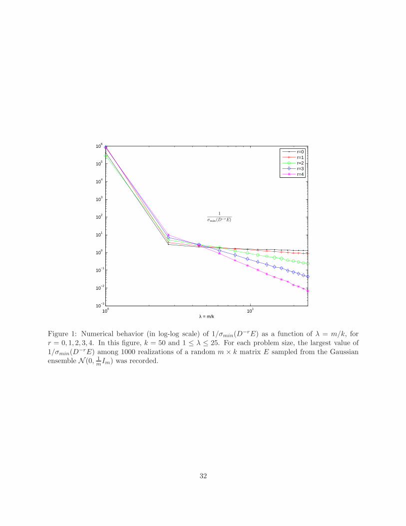
100

101

10−3

10−2

10−1

100

101

102

103

104

105

106

λ = m/k

1

σmin(D−rE)

r=0r=1r=2r=3r=4

Figure 1: Numerical behavior (in log-log scale) of 1/σmin(D−rE) as a function of λ = m/k, for

r = 0, 1, 2, 3, 4. In this figure, k = 50 and 1 ≤ λ ≤ 25. For each problem size, the largest value of1/σmin(D

−rE) among 1000 realizations of a random m × k matrix E sampled from the Gaussianensemble N (0, 1

mIm) was recorded.

32

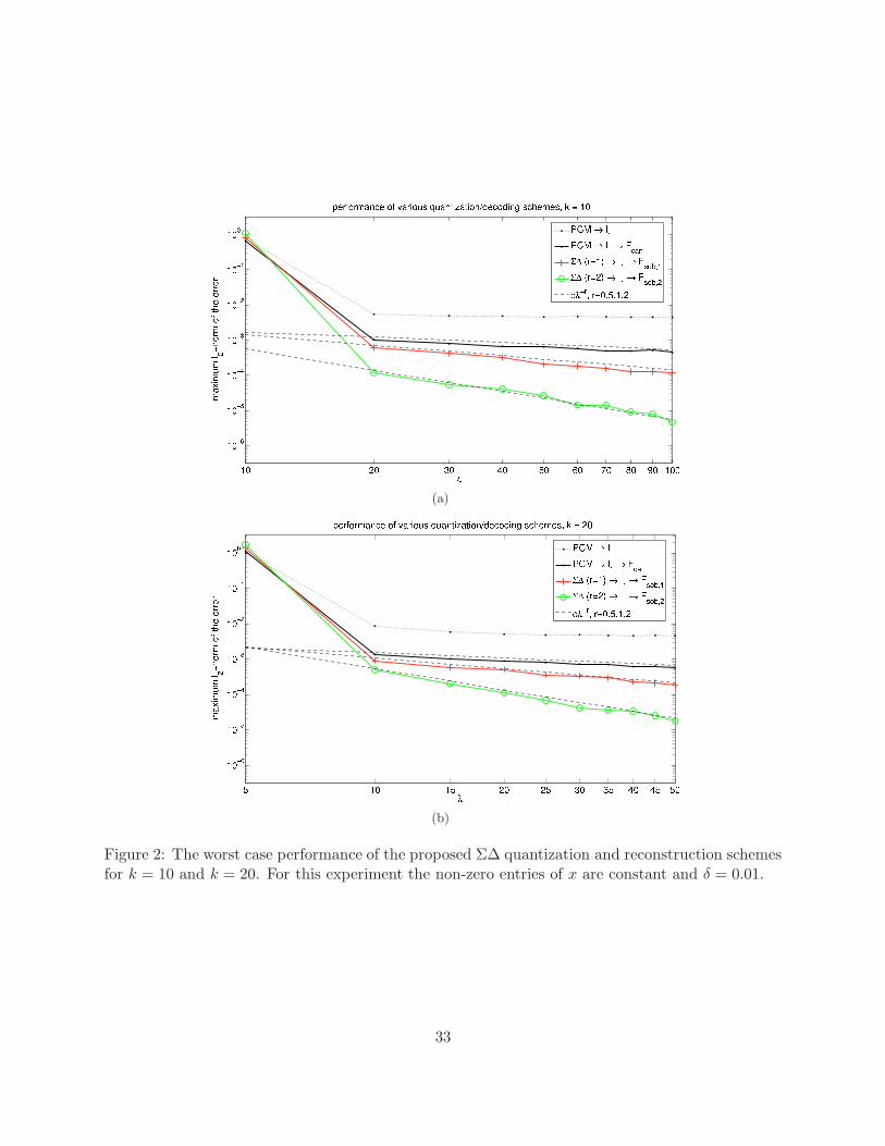
(a)

(b)

Figure 2: The worst case performance of the proposed Σ∆ quantization and reconstruction schemesfor k = 10 and k = 20. For this experiment the non-zero entries of x are constant and δ = 0.01.

33

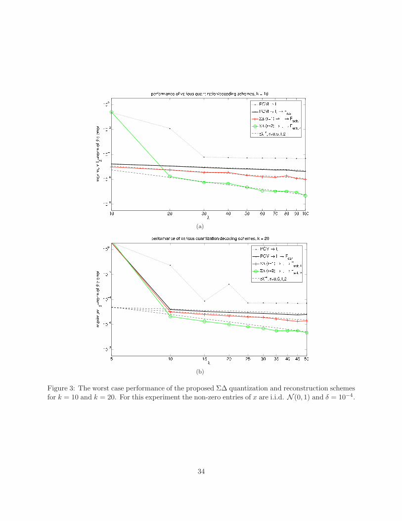
(a)

(b)

Figure 3: The worst case performance of the proposed Σ∆ quantization and reconstruction schemesfor k = 10 and k = 20. For this experiment the non-zero entries of x are i.i.d. N (0, 1) and δ = 10−4.

34

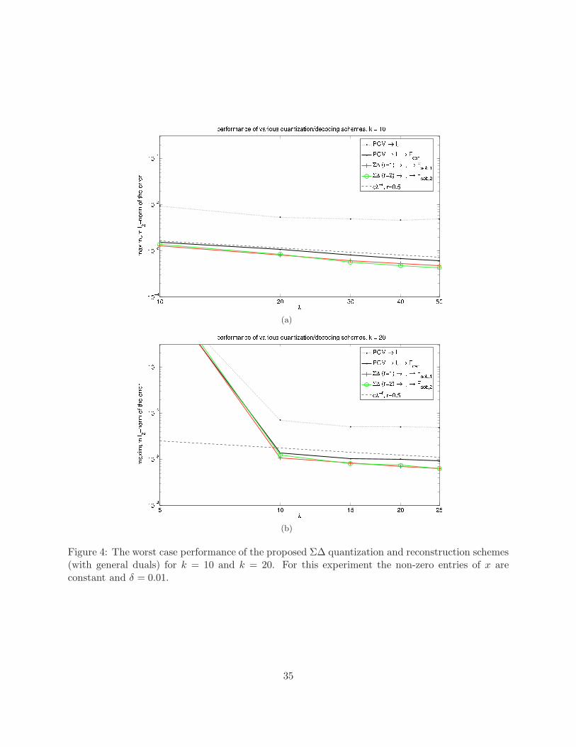
(a)

(b)

Figure 4: The worst case performance of the proposed Σ∆ quantization and reconstruction schemes(with general duals) for k = 10 and k = 20. For this experiment the non-zero entries of x areconstant and δ = 0.01.

35