Smooth Conformal α-NEM for Gradient...
27
Smooth Conformal α-NEM for Gradient Elasticity A. Rajagopal a , M. Scherer a , P. Steinmann a,∗ , N. Sukumar b a Chair of Applied Mechanics, University of Erlangen-Nuremberg, Eagerlandstraße 5, D-91058 Erlangen, Germany. b Department of Civil and Environmental Engineering, University of California, One Shields Avenue, Davis, CA 95616 USA. Abstract Strain gradient theory for continuum analysis has kinematic relations, which include terms from second gradients of the deformation map. This results in balance equations that have fourth order spatial derivatives, supple- mented with higher order boundary conditions. The weak formulation of fourth order operators stipulate that the basis functions must be globally C 1 continuous; very few finite elements in two dimensions meet this require- ment. In this paper, we propose a meshfree methodology for the analysis of gradient continua using a conformal α-shape based natural element method (NEM). The conformal α-NEM allows the construction of models entirely in terms of nodes, and ensures quadratic precision of the interpolant over convex and non-convex boundaries. Smooth natural neighbor interpolants are achieved by a transformation of Farin’s C 1 interpolant, which are obtained by embedding Sibson’s natural neighbor coordinates in the Bernstein-B´ ezier surface representation of a cubic simplex. Numerical examples are presented to demonstrate the accuracy and efficiency of the proposed method. 1. Introduction It is well-known that inhomogeneities present in any material at the microscopic scale influence its properties at the macroscopic scale: materials such as suspensions, blood flows, liquid crystals, porous media, polymeric substances, solids with microcracks, dislocations, turbulent fluids with vortices, and composites point to the need for incorporating micro motions in continuum mechanical formulations. There has been considerable focus towards the development of gradient continuum theories that account for the inherent microstructure in such natural and engineering materials. The notion of generalized continua unifies several extended continuum the- ories that account for such a size dependence due to the underlying microstructure of the material. These can be categorized as gradient continuum theories (see Mindlin and Tiersten (1962), Mindlin (1965), Mindlin and Tiersten (1964)), micro continuum theories (see Eringen (1964), Eringen (1970) and Hirschberger and Steinmann (2007)), and nonlocal continuum theories. In gradient continuum theory, on associating tensors of various order with material points, higher order theories can be constructed (see Eringen (1998), Eringen (1992)). In this paper, the focus is on developing a computational methodology for solving a gradient continuum formula- tion. In particular, we consider the strain gradient theory, or the gradient continuum as for example the second gradient of strain model as given by Toupin (1962) and Mindlin (Mindlin and Tiersten (1962), Mindlin (1965), Mindlin and Tiersten (1964)). Strain gradient theory requires no additional degrees of freedom but imposes C 1 continuity requirements. A comparison of various higher order gradient theories can be found in Fleck and ∗ Corresponding author Email address: [email protected] (P. Steinmann) INTERNATIONAL JOURNAL OF STRUCTURAL CHANGES IN SOLIDS – Mechanics and Applications Volume 1, Number 1, December 2009, pp. 83-109
-
Upload
vuongtuong -
Category
Documents
-
view
213 -
download
0
Transcript of Smooth Conformal α-NEM for Gradient...
Smooth Conformal α-NEM for Gradient Elasticity
A. Rajagopala, M. Scherera, P. Steinmanna,∗, N. Sukumarb
aChair of Applied Mechanics, University of Erlangen-Nuremberg, Eagerlandstraße 5, D-91058 Erlangen, Germany.bDepartment of Civil and Environmental Engineering, University of California, One Shields Avenue, Davis, CA 95616 USA.
Abstract
Strain gradient theory for continuum analysis has kinematic relations, which include terms from second gradientsof the deformation map. This results in balance equations that have fourth order spatial derivatives, supple-mented with higher order boundary conditions. The weak formulation of fourth order operators stipulate thatthe basis functions must be globally C1 continuous; very few finite elements in two dimensions meet this require-ment. In this paper, we propose a meshfree methodology for the analysis of gradient continua using a conformalα-shape based natural element method (NEM). The conformal α-NEM allows the construction of models entirelyin terms of nodes, and ensures quadratic precision of the interpolant over convex and non-convex boundaries.Smooth natural neighbor interpolants are achieved by a transformation of Farin’s C1 interpolant, which areobtained by embedding Sibson’s natural neighbor coordinates in the Bernstein-Bezier surface representation ofa cubic simplex. Numerical examples are presented to demonstrate the accuracy and efficiency of the proposedmethod.
1. Introduction
It is well-known that inhomogeneities present in any material at the microscopic scale influence its propertiesat the macroscopic scale: materials such as suspensions, blood flows, liquid crystals, porous media, polymericsubstances, solids with microcracks, dislocations, turbulent fluids with vortices, and composites point to theneed for incorporating micro motions in continuum mechanical formulations. There has been considerable focustowards the development of gradient continuum theories that account for the inherent microstructure in suchnatural and engineering materials. The notion of generalized continua unifies several extended continuum the-ories that account for such a size dependence due to the underlying microstructure of the material. These canbe categorized as gradient continuum theories (see Mindlin and Tiersten (1962), Mindlin (1965), Mindlin andTiersten (1964)), micro continuum theories (see Eringen (1964), Eringen (1970) and Hirschberger and Steinmann(2007)), and nonlocal continuum theories. In gradient continuum theory, on associating tensors of various orderwith material points, higher order theories can be constructed (see Eringen (1998), Eringen (1992)).In this paper, the focus is on developing a computational methodology for solving a gradient continuum formula-tion. In particular, we consider the strain gradient theory, or the gradient continuum as for example the secondgradient of strain model as given by Toupin (1962) and Mindlin (Mindlin and Tiersten (1962), Mindlin (1965),Mindlin and Tiersten (1964)). Strain gradient theory requires no additional degrees of freedom but imposesC1 continuity requirements. A comparison of various higher order gradient theories can be found in Fleck and
∗Corresponding authorEmail address: [email protected] (P. Steinmann)
INTERNATIONAL JOURNAL OF STRUCTURAL CHANGES IN SOLIDS – Mechanics and Applications Volume 1, Number 1, December 2009, pp. 83-109
84 Rajagopal et al. / International Journal of Structural Changes in Solids 1(2009)
Hutchinson (1996). The present work draws from the contribution of Kirchner and Steinmann (2007), where thevariational concepts on gradient and micromorphic continuum have been presented. A more detailed formulationof a gradient approach in spatial and material setting appears in Kirchner and Steinmann (2005) and in Sunykand Steinmann (2003). The balance equations for a gradient continuum have fourth order spatial derivativesanalogous to the biharmonic equation of Kirchhoff plates together with higher order boundary conditions. Thesolution of these equations require that the primary variable be C1 continuous; only a few two dimensionalfinite elements that have been developed for plate bending problems meet this requirement. The most commonway for gradient continuum analysis has been through the use of mixed formulations using finite elements (Shuet al. (1999), Amanatdou and Aravas (2002)), that only requires C0 continuity (see Kouznetsova (2002) andKouznetsova et al. (2004)). All these methods lead to extra degrees of freedom in addition to the primaryunknowns. The formulation of C1 finite elements has significant complexity (Stogner and Carey (2007)). Analternative choice with higher order approximants is the use of a meshfree method like the element-free Galerkin(Belytschko et al. (1994), Askes and Aifantis (2002)) or the meshless local Petrov Galerkin (see Tang et al.(2003)). Most of these methods are for small strains and they pose difficulties in the imposition of boundaryconditions because of the non-interpolating property of the approximant.The natural element method (NEM), which is based on Sibson’s C0 interpolant (Sibson, 1980, 1981) was proposedby Braun and Sambridge (1995). It was used for data approximation in geophysical applications (Sambridgeet al., 1995), and also successfully explored for solid mechanics problems by Sukumar et al. (1998). Farin pro-posed a C1 natural neighbor interpolant (Farin, 1990), which was used by Sukumar and Moran (1999) to solvefourth-order elliptic boundary-value problems. Farin’s C1 interpolant is obtained by embedding Sibson’s naturalneighbor coordinates in the Bernstein-Bezier surface representation of a cubic simplex (see Farin (1986)), andthe transformation adopted by Sukumar and Moran (1999) led to interpolation of nodal function and nodalgradient values. The interpolation property makes the C1 NEM a suitable candidate for use in the Galerkinimplementation of gradient continua. The α-shape based extension of NEM by Cueto et al. (2002) enabledthe construction of models entirely in terms of nodes and the imposition of essential boundary conditions onnon-convex parts of the boundary (Cueto et al. (2000)). The use of a conformal α- shapes (Cazals et al. (2006)),helps in recovering the whole domain from a discrete set of nodes.In this paper, a methodolgy for solving a gradient continuum formulation is presented. The kinematics are pre-sented for finite deformations, which include the first and second order gradient terms. For conservative staticproblems, the Dirichlet principle results in the Euler-Lagrange equations, i.e., the balance of momentum in itsstrong form. Thus, upon the definition of proper gradient elasticity kinematics, in terms of incorporation of thehigher order deformation gradient contribution, a variation of the potential energy renders the weak form of thebalance of the momentum together with Neumann boundary conditions and higher order boundary conditionsin terms of double force terms. A solution to these equations is presented through the C1 conformal α-naturalelement method.The remainder of this paper is organized as follows. In the next section, we present the kinematics of gradientcontinua for a geometrically nonlinear setting and the constitutive formulation that includes the length scaleeffects in the energy expression. Natural neighbor interpolation is introduced in Section 3 and the trial andtest approximations used in the C1 NEM for gradient elasticity are presented in Section 4. The extension to aconformal α-shape based natural element method follows thereafter in Section 5. In Section 6, several numericalexamples are presented to demonstrate the accuracy of the method, and we close with a few concluding remarksin Section 7.
2. Gradient Continua
2.1. Kinematic relations
To investigate the variational principle in a geometrically nonlinear setting we refer all quantities arising inthe continuum mechanical description to the material configuration B0 ⊂ �3 with boundary ∂B0 and outwardunit normal vector N . In defining the motion of B0 a typical continuum particle occupies a succession of points
Rajagopal et al. / Smooth Conformal α-NEM for Gradient Elasticity 85
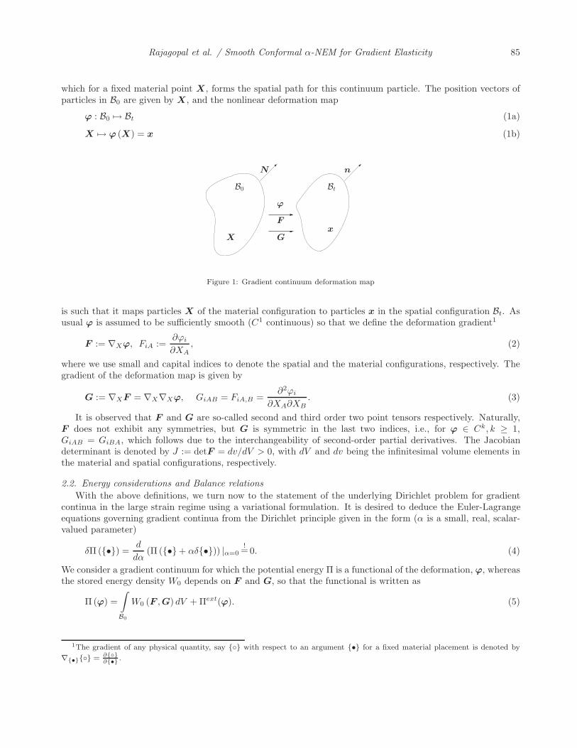
which for a fixed material point X, forms the spatial path for this continuum particle. The position vectors ofparticles in B0 are given by X, and the nonlinear deformation map
ϕ : B0 �→ Bt (1a)
X �→ ϕ (X) = x (1b)
B0 Bt
Xx
ϕ
F
G
N n
Figure 1: Gradient continuum deformation map
is such that it maps particles X of the material configuration to particles x in the spatial configuration Bt. Asusual ϕ is assumed to be sufficiently smooth (C1 continuous) so that we define the deformation gradient1
F := ∇Xϕ, FiA :=∂ϕi
∂XA, (2)
where we use small and capital indices to denote the spatial and the material configurations, respectively. Thegradient of the deformation map is given by
G := ∇XF = ∇X∇Xϕ, GiAB = FiA,B =∂2ϕi
∂XA∂XB. (3)
It is observed that F and G are so-called second and third order two point tensors respectively. Naturally,F does not exhibit any symmetries, but G is symmetric in the last two indices, i.e., for ϕ ∈ Ck, k ≥ 1,GiAB = GiBA, which follows due to the interchangeability of second-order partial derivatives. The Jacobiandeterminant is denoted by J := detF = dv/dV > 0, with dV and dv being the infinitesimal volume elements inthe material and spatial configurations, respectively.
2.2. Energy considerations and Balance relationsWith the above definitions, we turn now to the statement of the underlying Dirichlet problem for gradient
continua in the large strain regime using a variational formulation. It is desired to deduce the Euler-Lagrangeequations governing gradient continua from the Dirichlet principle given in the form (α is a small, real, scalar-valued parameter)
δΠ({•}) =d
dα(Π ({•}+ αδ{•})) |α=0
!= 0. (4)
We consider a gradient continuum for which the potential energy Π is a functional of the deformation, ϕ, whereasthe stored energy density W0 depends on F and G, so that the functional is written as
Π (ϕ) =∫B0
W0 (F ,G) dV + Πext(ϕ). (5)
1The gradient of any physical quantity, say {◦} with respect to an argument {•} for a fixed material placement is denoted by
∇{•}{◦} = ∂{◦}∂{•} .
86 Rajagopal et al. / International Journal of Structural Changes in Solids 1(2009)
If we assume the material to be hyperelastic, stresses can be defined as the derivatives of W0 with respect totheir energetically conjugate deformation variables. The macro-stress P , and the double stress Q of Piola typetogether with the volume force density b0 are obtained by the derivatives2
P := DFW0, Q := DGW0, b0 := DϕW0 (6)
For arbitrary variations of δϕ, the energy minimization takes the form3
δΠ =∫B0
[P : δF + Q
...δG]dV + δΠext = 0, (7)
where
Πext := −∫B0
b0 · ϕdV −∫
∂B0
ϕ · tP0 dA−
∫∂B0
∇(N)X ϕ · tQ
0 dA. (8)
In the above equation, b0 is the body force density acting on the material domain B0. tP0 and tQ
0 are thenominal surface traction and second-order stress traction, respectively, which act on the surface in the materialconfiguration ∂B0 (see Mindlin (1965)). By application of Gauss’s theorem, we derive the higher order equilibriumequations and Neumann type boundary conditions4
Div (P − Div Q) = −b0 in B0 (9)
[P − Div Q] · N + L(Q · N) = tP0 on ∂B0 (10)
Q : [N ⊗ N ] = tQ0 on ∂B0 (11)
where L(Q · N) denotes the following differential operator
−L(Q · N ) = KQ : [N ⊗ N ] + ∇(T )X (Q · N) : I (12)
with the total curvature K = −∇(T )X N : I of the surface ∂B0. Herein ∇(N)
X and ∇(T )X denote the normal and
tangential components of the gradient. A detailed derivation of these equations is presented in the Appendix.
2.3. Piola transform of the balance of momentum
To establish the balance of linear momentum in material parameterization and spatial reference a one-sidedpush forward – a Piola transformation – is applied to the balance of momentum, Eq. (9), in order to rewritethem in terms of purely spatial stress tensors. For this purpose the Piola transformation formulae
{•} �→ j{•} · F T (13)
is used with j = 1/J = dV/dv, as the inverse Jacobian determinant. Eq. (13) relates Div({•}) = Jdiv(j{•}·F T ),the divergence operator Div({•}) with respect to material placement to the divergence operator with respect to
2The derivatives of values with respect to tensors of any order are denoted by ∂{•}{◦} = ∂{◦}∂{•} . Additionally for the sake of
clarity, D{•}{◦} = ∂{◦}∂{•}
⏐⏐⏐X
denotes the derivative with respect to a variable at fixed material placement X.
3Here : denotes a double contraction of rank-two tensors P and F , i.e., PiJFiJ and... denotes a triple contraction of rank-three
tensors Q and G, i.e., QiJKGiJK .4The divergence operators identify as: Div ({•}) := ∇X{•} : I, with respect to material coordinates X.
Rajagopal et al. / Smooth Conformal α-NEM for Gradient Elasticity 87
the spatial placement div({•}). With this transformation, we obtain the (gradient enhanced) Cauchy stress andconvected hyperstress5 as
σ := j[P · F T + Q
2,3: G
]and τ = jQ :
[F T⊗F T
](14)
On using the divergence relation Div (P − DivQ) = J div(j [P − DivQ] · F T ) and also j [DivQ] · F T =
div( jQ :[F T⊗F T
]) − jQ
2,3: G and jb0 = bt, the balance of linear momentum with material parameterization
and spatial reference is given by 6
div(σ − div τ ) = −bt. (15)
2.4. Constitutive assumption for stored energy density
A hyperelastic constitutive theory is chosen. The constitutive relation is appropriately chosen including alength scale parameter l. Using this constitutive assumption, various stress measures are derived for the spatialmotion problem. For the internally stored energy density W0, we assume the following hyperelastic constitutivefunction
W0 (F ,G) =12λ ln2 J +
12μ
[F : F − ndim − 2 lnJ
]+
12μl2G
...G, (16)
which consists of a Neo-Hookean term and an additional length scale term which takes into account the second-order gradients. Herein, the material parameters λ and μ are the Lame constants from classical elasticity.Additionally, the so called internal length l, accounts for the scale dependence and may be interpreted as acharacteristic size at the corresponding length. Furthermore, ndim denotes the number of space dimensions.With this constitutive assumption the Piola type stresses take the form
P = DFW0 = [λ lnJ − μ] F−T + μF , (17a)
Q = DGW0 = μl2G. (17b)
Moreover, the Cauchy type stresses are eventually evaluated as
σ = j[[λ ln J − μ] F−T + μF
]· F T + jμl2G
2,3: G, (18a)
τ = jμl2G :[F T⊗F T
](18b)
3. C1 natural neighbor interpolation
It is evident from Eq. (9) to Eq. (12) that the balance of momentum equation is of fourth order and requiresan approximation which is C1 continuous. To achieve this in the present work we pursue an implementation ofgradient continua using the conformal α-natural element method (hereafter, as in Cueto et al. (2000), we referto it as α-NEM). The α-NEM allows the construction of models entirely in terms of nodes, reproduces the wholedomain and also ensures quadratic precision of the interpolant over convex and non-convex boundaries. A briefdescription of C0 and C1 natural neighbor interpolation schemes follows.
5Q2,3: G denotes a double contraction of two rank three tensors with respect to the second and third index i.e., QaJKGbJK
6The regular and modified dyadic products of two second order tensors are defined through the relations[A⊗ B] : C = [B : C] A, A : [B ⊗ C] = [A : B] C[A⊗B
]: C = A · C · BT , A :
[B⊗C
]= BT · A · C[
A⊗B]
: C = A · CT · BT , A :[B⊗C
]= BT · AT · C
88 Rajagopal et al. / International Journal of Structural Changes in Solids 1(2009)
(a) (b)
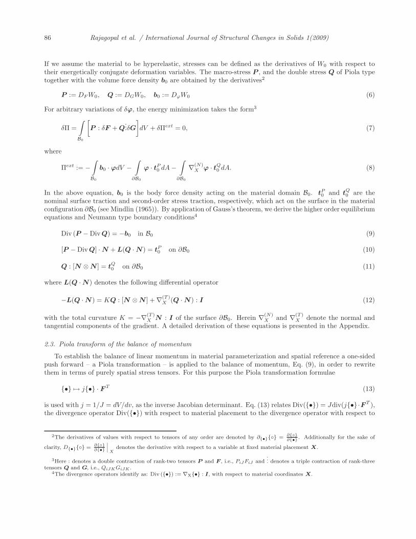
Figure 2: (a) First order Voronoi diagram and Delaunay triangulation of a set of five points; and (b) Second-order Voronoi andSibson interpolant of p′ with respect to node 2.
Consider a set of nodes N = {n1, n2, . . . , nM} ∈ �2. Natural neighbor coordinates are constructed on thebasis of the underlying Voronoi tessellation for the nodal set N . The first order Voronoi diagram of the set N isa subdivision of the plane into cells VI (Voronoi polygons) such that any point in VI is closer to node nI than toany other node nJ ∈ N :
VI ={X ∈ �2 : d(X ,XI) < d(X,XJ ) ∀J �= I
}(19)
where d(·, ·), the Euclidean metric, is the distance between XI and XJ . The first-order Voronoi diagram, itsdual the Delaunay triangulation, and the empty circumcircles for the set N are shown in Figure 2a. Now apoint p′ is introduced into the Voronoi diagram of set N . If p′ is tessellated along with the nodal set N , then,in the newly constructed triangulation based on N and p′, the natural neighbors of p′ are those nodes that areconnected by a Delaunay edge to p′. The C0 natural neighbor interpolant of p′ with respect to the naturalneighbor node 2 is defined as the ratio of the area of overlap of the Voronoi cell, V2p′ , to the total area of theVoronoi cell of p′, that is
φ2(p′) =area (defg)area (abcde)
=A2(p′)A(p′)
. (20)
Thus, for any natural neighbor node I, the ratio of the area of overlap of the Voronoi cells to the total area ofthe Voronoi cell of p′ is
φI(p′) =AI(p′)A(p′)
, (21)
where
A(p′) =n∑
I=1
AI(p′). (22)
To achieve C1 natural neighbor interpolation, we adopt the procedure proposed by Sukumar and Moran (1999).The methodology is based on embedding the C0 natural neighbor interpolant in the Bernstein-Bezier representa-tion of a cubic simplex, termed as Farin’s interpolant (see Farin (1990)) and performing a simple transformationto relate the Bezier ordinates to the nodal degrees of freedom. Let the point p′ ∈ Ω ⊂ �2 have n naturalneighbors, with φI(p′) as the natural neighbor interpolant of node I (I = 1, n). Let this set be defined byΦ = (φ1(p′), φ2(p′), φ3(p′)......φn(p′)). These C0 natural neighbor interpolants are identical to the barycentric

Rajagopal et al. / Smooth Conformal α-NEM for Gradient Elasticity 89
coordinates of a simplex δ ∈ �n−1. Following a multi-index notation7, a Bernstein-Bezier cubic surface (m = 3)over the simplex δ can be written in the form
w3 (Φ) =∑|i|=3
B3i (Φ)bi, (23)
which is the C1 interpolant used as a trial function in the natural element method. In the above equation,B3
i (Φ) =(3i
)φi1
1 φi22 ........φ
inn , where |i| = i1 + i2 + i3 + . . . + in = 3. The Bezier ordinate bi is associated with
the control point qi ∈ �2, where qi are the projection of control points of m-variate Bezier polynomials over then− 1 dimensional simplex on to the plane
qi =∑|j|=1
B1j (i/3)Xj, |i| = 3 (24)
For more details on Bernstein-Bezier representation the reader can refer to Farin (1985). Following the procedureoutlined in Sukumar and Moran (1999), now the C1 interpolant, which is a function of Bezier ordinates, asgiven in Eq. (23), is transformed to a function of nodal function values and nodal gradient values by a simpletransformation of the form
wh (Φ) = {B(Φ)}T {b} = {B(Φ)}T [T ] {w} = {Ψ (Φ)}T {w} . (25)
On constructing the transformation matrix [T ] (see Sukumar and Moran (1999) for more details), we can expressthe C1(Ω) NEM trial function in standard shape function notation as
wh (p′) =3n∑
J=1
ψJ (p′) dJ , (26)
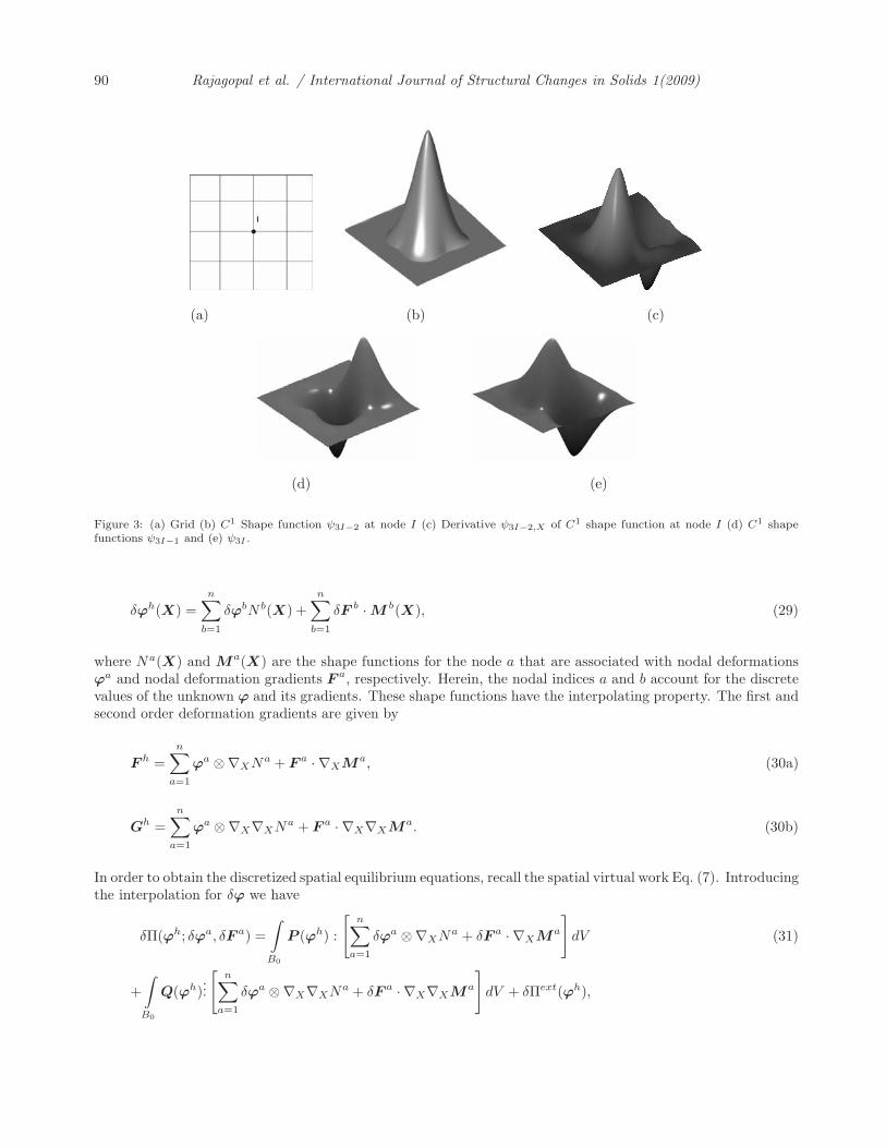
where ψ3I−2(p′), ψ3I−1(p′), and ψ3I(p′) are the shape functions of node I that are associated with the dJ given bydJ = {d3I−2, d3I−1, d3I} = {wI , wI,X , wI,Y }, which is a function of nodal function values wI and nodal gradientvalues wI,X and wI,Y . The C1 shape functions are shown in Figure 3.
Most of the properties of the C0(Ω) natural neighbor shape functions and Bernstein-Bezier shape functionsare retained by C1(Ω) shape functions. C1(Ω) NEM shape functions posses properties such as partition of unity,quadratic completeness, positivity and interpolation. The C1 NEM interpolant interpolates to nodal functionvalues and nodal gradient values, and this property makes it a suitable candidate for use in a gradient continuumformulation.
ψ3I−2(XJ ) = δIJ ψ3I−1(XJ ) = 0 ψ3I(XJ ) = 0ψ3I−2,X(XJ ) = 0 ψ3I−1,X(XJ ) = δIJ ψ3I,X(XJ ) = 0ψ3I−2,Y (XJ ) = 0 ψ3I−1,Y (XJ ) = 0 ψ3I,Y (XJ ) = δIJ (27)
4. C1 natural element method for gradient continua
Equation (Eq. (9) - Eq. (12)) is a fourth order equation analogous to the biharmonic equation of Kirchoffplates. The solution to this equation thus requires C1 continuous approximations. To this end, we use the C1
natural neighbour approximation, both for the deformation map and for the space of admissible variations.Now, for a gradient continuum, we write the C1 natural neighbour approximation as a sum of deformation
and gradients of deformation degrees of freedom given by
ϕh(X) =n∑
a=1
ϕaNa(X) +n∑
a=1
F a · Ma(X), (28)
7Multi-indices are n-tuples of nonnegative integers, the components of which start at zero; with the norm defined as |i| = m =i1 + i2 + ....+ in.
90 Rajagopal et al. / International Journal of Structural Changes in Solids 1(2009)
(a) (b) (c)
(d) (e)
Figure 3: (a) Grid (b) C1 Shape function ψ3I−2 at node I (c) Derivative ψ3I−2,X of C1 shape function at node I (d) C1 shapefunctions ψ3I−1 and (e) ψ3I .
δϕh(X) =n∑
b=1
δϕbN b(X) +n∑
b=1
δF b · Mb(X), (29)
where Na(X) and Ma(X) are the shape functions for the node a that are associated with nodal deformationsϕa and nodal deformation gradients F a, respectively. Herein, the nodal indices a and b account for the discretevalues of the unknown ϕ and its gradients. These shape functions have the interpolating property. The first andsecond order deformation gradients are given by
F h =n∑
a=1
ϕa ⊗∇XNa + F a · ∇XMa, (30a)
Gh =n∑
a=1
ϕa ⊗∇X∇XNa + F a · ∇X∇XMa. (30b)
In order to obtain the discretized spatial equilibrium equations, recall the spatial virtual work Eq. (7). Introducingthe interpolation for δϕ we have
δΠ(ϕh; δϕa, δF a) =∫B0
P (ϕh) :
[n∑
a=1
δϕa ⊗∇XNa + δF a · ∇XMa
]dV (31)
+∫B0
Q(ϕh)...
[n∑
a=1
δϕa ⊗∇X∇XNa + δF a · ∇X∇XMa
]dV + δΠext(ϕh),

Rajagopal et al. / Smooth Conformal α-NEM for Gradient Elasticity 91
The above equation can be rearranged for all δϕa and δF a as
δΠ(ϕh; δϕa, δF a) =n∑
a=1
δϕa ·∫B0
[P (ϕh) · ∇XN
a + Q(ϕh) : ∇X∇XNa]dV (32)
+n∑
a=1
δF a :∫B0
[P (ϕh)
2· ∇XMa + Q(ϕh)2,3: ∇X∇XMa
]dV + δΠext(ϕh) = 0.
The discrete residuals8 of the spatial motion problem can thus be written as
Rϕa =
∫B0
P (ϕh) · ∇XNa(X)dV +
∫B0
Q(ϕh
): ∇X∇XN
a (X) dV − F ϕext
a = 0. (33a)
RFa =
∫B0
P (ϕh)2· ∇XMa(X)dV +
∫B0
Q(ϕh)2,3: ∇X∇XMa(X)dV − F F ext
a = 0. (33b)
This represents a set of nonlinear equilibrium equations with the current nodal deformation and its gradientas unknowns. The solution of these equations is achieved using a Newton Raphson iterative procedure. Thelinearized coupled problem
[Kϕϕ
ab KϕFab
KFϕab KFF
ab
] [Δϕb
ΔF b
]=
[F ϕext
a − F ϕint
a
F F ext
a − F F int
a
]
is solved for increments of ϕb and F b. The component matrices of the global tangent stiffness matrix are givenby
Kϕϕab =
∂Rϕa
∂ϕb
=∫B0
[[DF P · ∇XN
a] · ∇XNb + [DGQ : ∇X∇XN
a] : ∇X∇XNb]dV (34a)
KϕFab =
∂Rϕa
∂F b=
∫B0
[[DF P · ∇XN
a]2· ∇XM b + [DGQ : ∇X∇XN
a]2,3: ∇X∇XM b
]dV (34b)
KFϕab =
∂RFa
∂ϕb
=∫B0
[[DF P · ∇XMa]
2· ∇XNb + [DGQ : ∇X∇XMa]
2,3: ∇X∇XN
b]dV (34c)
KFFab =
∂RFa
∂F b=
∫B0
[[DF P · ∇XMa]
2· ∇XM b + [DGQ : ∇X∇XMa]2,3: ∇X∇XM b
]dV (34d)
where the specific tangent operators for the constitutive law read as
DF P = λF−T ⊗ F−T − [λ lnJ − μ] F−T⊗F−T + [μ] I⊗I (35a)
DGQ = μl2I⊗ [I⊗I] , (35b)
where DF P and DGQ are tensors of fourth and sixth order respectively. Kϕϕab ,KϕF
ab and its symmetric counter-part KFϕ
ab and KFFab are tensors of second, third, and fourth order respectively and are arranged in appropriate
global locations to yield the global stiffness matrix. The symmetric bilinear form of basis functions togetherwith continous function of nodal function values and nodal gradient values in the neighbourhood of any givenevaluation point result in symmetric hessian matrix. A background cell grid with standard Gauss quadraturerule is used for numerical evaluation of these integrals.
8A2· B denotes a contraction of rank two tensors with respect to the second index i.e., AaJBbJ
92 Rajagopal et al. / International Journal of Structural Changes in Solids 1(2009)
5. On the α-shape extension to NEM
So called α-shapes define a family of simplicial complexes parameterized by α ∈ R. This concept was intro-duced by Edelsbrunner et al. (1983), for the study of points in the plane and higher dimensions by Edelsbrunnerand Mucke (1994). Recently, density scaled α-shapes have been used in natural neighbor interpolation forimposing essential boundary conditions on non-convex domains (Cueto et al., 2000). For non-uniform nodaldiscretization, there is a need for α shape filtration on a local scale, unlike a global scale for reconstructing thewhole domain. This requires a judicious choice of α values. Conformal alpha shapes (originally proposed byCazals et al. (2006)) are a potential solution for such discretizations. Let us consider a nodal point set S ⊂ R
d.For a given value of α ∈ [0,∞), α− balls are circles of radius α around the nodal points in S. The step by stepprocedure for construction of conformal α-shapes is briefly outlined here.
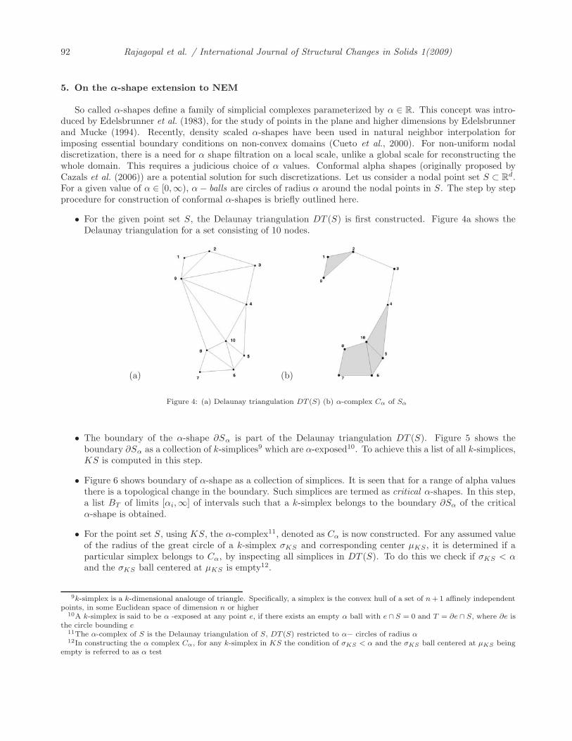
• For the given point set S, the Delaunay triangulation DT (S) is first constructed. Figure 4a shows theDelaunay triangulation for a set consisting of 10 nodes.
(a) (b)
Figure 4: (a) Delaunay triangulation DT (S) (b) α-complex Cα of Sα
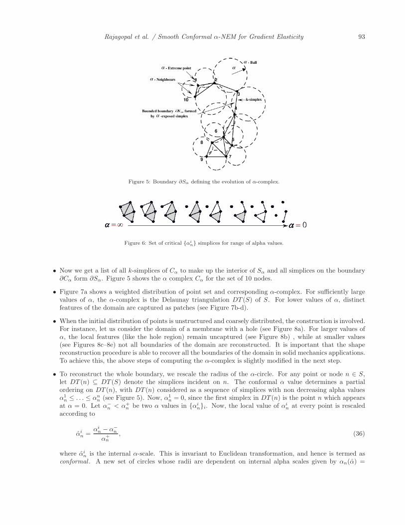
• The boundary of the α-shape ∂Sα is part of the Delaunay triangulation DT (S). Figure 5 shows theboundary ∂Sα as a collection of k-simplices9 which are α-exposed10. To achieve this a list of all k-simplices,KS is computed in this step.
• Figure 6 shows boundary of α-shape as a collection of simplices. It is seen that for a range of alpha valuesthere is a topological change in the boundary. Such simplices are termed as critical α-shapes. In this step,a list BT of limits [αi,∞] of intervals such that a k-simplex belongs to the boundary ∂Sα of the criticalα-shape is obtained.
• For the point set S, using KS, the α-complex11, denoted as Cα is now constructed. For any assumed valueof the radius of the great circle of a k-simplex σKS and corresponding center μKS , it is determined if aparticular simplex belongs to Cα, by inspecting all simplices in DT (S). To do this we check if σKS < αand the σKS ball centered at μKS is empty12.
9k-simplex is a k-dimensional analouge of triangle. Specifically, a simplex is the convex hull of a set of n+ 1 affinely independentpoints, in some Euclidean space of dimension n or higher
10A k-simplex is said to be α -exposed at any point e, if there exists an empty α ball with e ∩ S = 0 and T = ∂e ∩ S, where ∂e isthe circle bounding e
11The α-complex of S is the Delaunay triangulation of S, DT (S) restricted to α− circles of radius α12In constructing the α complex Cα, for any k-simplex in KS the condition of σKS < α and the σKS ball centered at μKS being
empty is referred to as α test
Rajagopal et al. / Smooth Conformal α-NEM for Gradient Elasticity 93
Figure 5: Boundary ∂Sα defining the evolution of α-complex.
Figure 6: Set of critical {αin} simplices for range of alpha values.
• Now we get a list of all k-simplices of Cα to make up the interior of Sα and all simplices on the boundary∂Cα form ∂Sα. Figure 5 shows the α complex Cα for the set of 10 nodes.
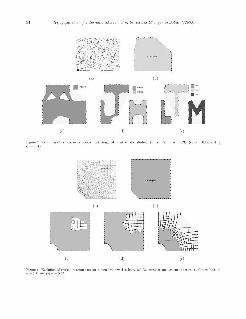
• Figure 7a shows a weighted distribution of point set and corresponding α-complex. For sufficiently largevalues of α, the α-complex is the Delaunay triangulation DT (S) of S. For lower values of α, distinctfeatures of the domain are captured as patches (see Figure 7b-d).
• When the initial distribution of points is unstructured and coarsely distributed, the construction is involved.For instance, let us consider the domain of a membrane with a hole (see Figure 8a). For larger values ofα, the local features (like the hole region) remain uncaptured (see Figure 8b) , while at smaller values(see Figures 8c–8e) not all boundaries of the domain are reconstructed. It is important that the shapereconstruction procedure is able to recover all the boundaries of the domain in solid mechanics applications.To achieve this, the above steps of computing the α-complex is slightly modified in the next step.
• To reconstruct the whole boundary, we rescale the radius of the α-circle. For any point or node n ∈ S,let DT (n) ⊆ DT (S) denote the simplices incident on n. The conformal α value determines a partialordering on DT (n), with DT (n) considered as a sequence of simplices with non decreasing alpha valuesα1
n ≤ . . . ≤ αnn (see Figure 5). Now, α1
n = 0, since the first simplex in DT (n) is the point n which appearsat α = 0. Let α−
n < α+n be two α values in {αi
n}i. Now, the local value of αin at every point is rescaled
according to
αin =
αin − α−
n
α+n
, (36)
where αin is the internal α-scale. This is invariant to Euclidean transformation, and hence is termed as
conformal . A new set of circles whose radii are dependent on internal alpha scales given by αn(α) =
94 Rajagopal et al. / International Journal of Structural Changes in Solids 1(2009)
(a) (b)
(c) (d) (e)
Figure 7: Evolution of critical α-complexes. (a) Weighted point set distribution; (b) α = 2; (c) α = 0.35; (d) α = 0.12; and (e)α = 0.035
(a) (b)
(c) (d) (e)
Figure 8: Evolution of critical α-complexes for a membrane with a hole. (a) Delaunay triangulation; (b) α = 1; (c) α = 0.12; (d)α = 0.1; and (e) α = 0.07.
Rajagopal et al. / Smooth Conformal α-NEM for Gradient Elasticity 95
α+n α+ α−
n is considered. The conformal α-shape complex is thus obtained by Delaunay triangulation of S,restricted to Cα.
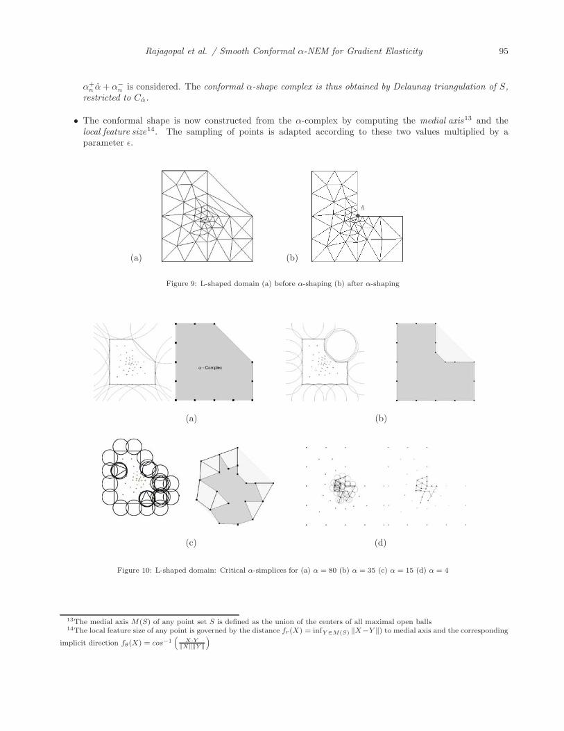
• The conformal shape is now constructed from the α-complex by computing the medial axis13 and thelocal feature size14. The sampling of points is adapted according to these two values multiplied by aparameter ε.
(a) (b)
Figure 9: L-shaped domain (a) before α-shaping (b) after α-shaping
(a) (b)
(c) (d)
Figure 10: L-shaped domain: Critical α-simplices for (a) α = 80 (b) α = 35 (c) α = 15 (d) α = 4
13The medial axis M(S) of any point set S is defined as the union of the centers of all maximal open balls14The local feature size of any point is governed by the distance fr(X) = infY ∈M(S) ‖X−Y ‖) to medial axis and the corresponding
implicit direction fθ(X) = cos−1(
X·Y‖X‖‖Y ‖
)
96 Rajagopal et al. / International Journal of Structural Changes in Solids 1(2009)
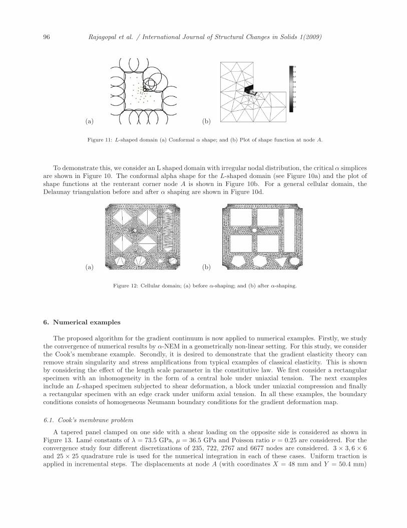
(a) (b)
Figure 11: L-shaped domain (a) Conformal α shape; and (b) Plot of shape function at node A.
To demonstrate this, we consider an L shaped domain with irregular nodal distribution, the critical α simplicesare shown in Figure 10. The conformal alpha shape for the L-shaped domain (see Figure 10a) and the plot ofshape functions at the renterant corner node A is shown in Figure 10b. For a general cellular domain, theDelaunay triangulation before and after α shaping are shown in Figure 10d.
(a) (b)
Figure 12: Cellular domain; (a) before α-shaping; and (b) after α-shaping.
6. Numerical examples
The proposed algorithm for the gradient continuum is now applied to numerical examples. Firstly, we studythe convergence of numerical results by α-NEM in a geometrically non-linear setting. For this study, we considerthe Cook’s membrane example. Secondly, it is desired to demonstrate that the gradient elasticity theory canremove strain singularity and stress amplifications from typical examples of classical elasticity. This is shownby considering the effect of the length scale parameter in the constitutive law. We first consider a rectangularspecimen with an inhomogeneity in the form of a central hole under uniaxial tension. The next examplesinclude an L-shaped specimen subjected to shear deformation, a block under uniaxial compression and finallya rectangular specimen with an edge crack under uniform axial tension. In all these examples, the boundaryconditions consists of homogeneous Neumann boundary conditions for the gradient deformation map.
6.1. Cook’s membrane problem
A tapered panel clamped on one side with a shear loading on the opposite side is considered as shown inFigure 13. Lame constants of λ = 73.5 GPa, μ = 36.5 GPa and Poisson ratio ν = 0.25 are considered. For theconvergence study four different discretizations of 235, 722, 2767 and 6677 nodes are considered. 3 × 3, 6 × 6and 25 × 25 quadrature rule is used for the numerical integration in each of these cases. Uniform traction isapplied in incremental steps. The displacements at node A (with coordinates X = 48 mm and Y = 50.4 mm)
Rajagopal et al. / Smooth Conformal α-NEM for Gradient Elasticity 97
Figure 13: Cook’s membrane problem
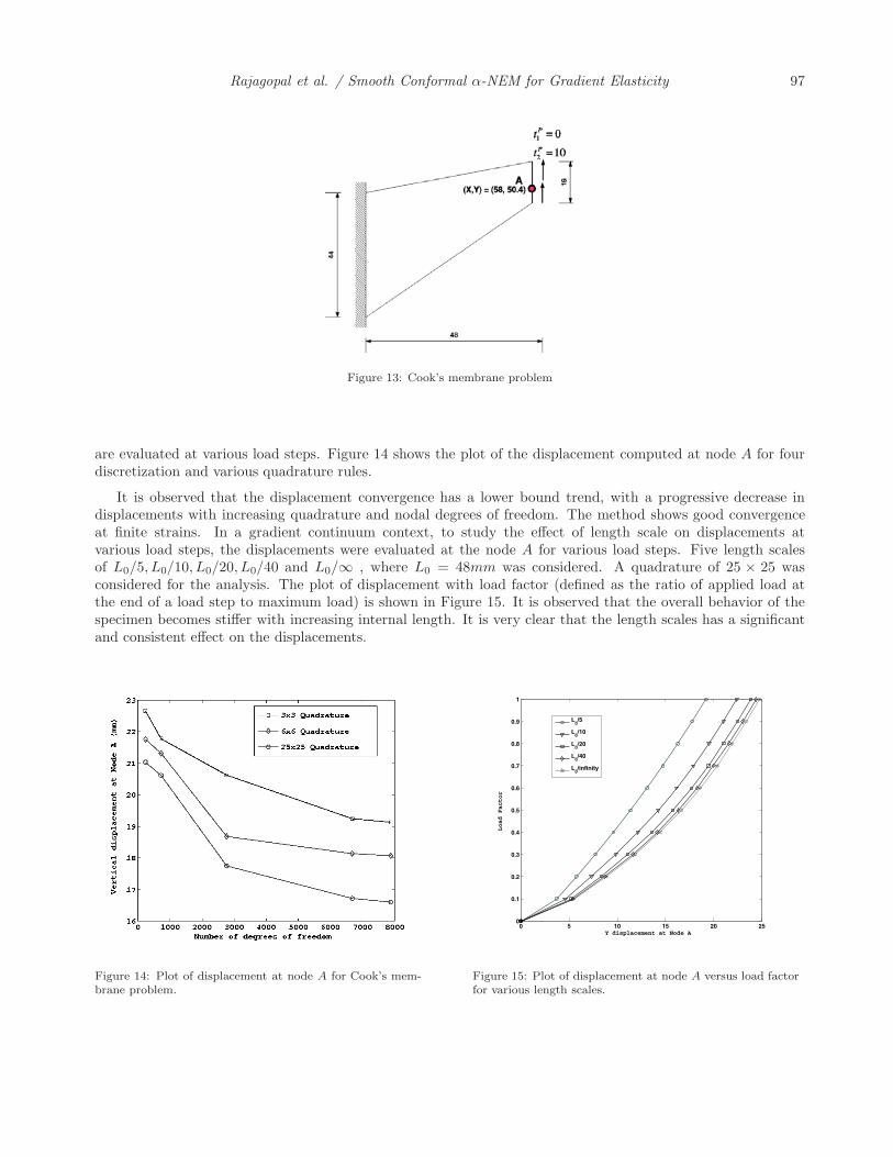
are evaluated at various load steps. Figure 14 shows the plot of the displacement computed at node A for fourdiscretization and various quadrature rules.
It is observed that the displacement convergence has a lower bound trend, with a progressive decrease indisplacements with increasing quadrature and nodal degrees of freedom. The method shows good convergenceat finite strains. In a gradient continuum context, to study the effect of length scale on displacements atvarious load steps, the displacements were evaluated at the node A for various load steps. Five length scalesof L0/5, L0/10, L0/20, L0/40 and L0/∞ , where L0 = 48mm was considered. A quadrature of 25 × 25 wasconsidered for the analysis. The plot of displacement with load factor (defined as the ratio of applied load atthe end of a load step to maximum load) is shown in Figure 15. It is observed that the overall behavior of thespecimen becomes stiffer with increasing internal length. It is very clear that the length scales has a significantand consistent effect on the displacements.
Figure 14: Plot of displacement at node A for Cook’s mem-brane problem.
0 5 10 15 20 250
0.1
0.2
0.3
0.4
0.5
0.6
0.7
0.8
0.9
1
Y displacement at Node A
Load Factor
L0/5
L0/10
L0/20
L0/40
L0/infinity
Figure 15: Plot of displacement at node A versus load factorfor various length scales.
98 Rajagopal et al. / International Journal of Structural Changes in Solids 1(2009)
6.2. Uniaxial loading of a rectangular specimen with a hole
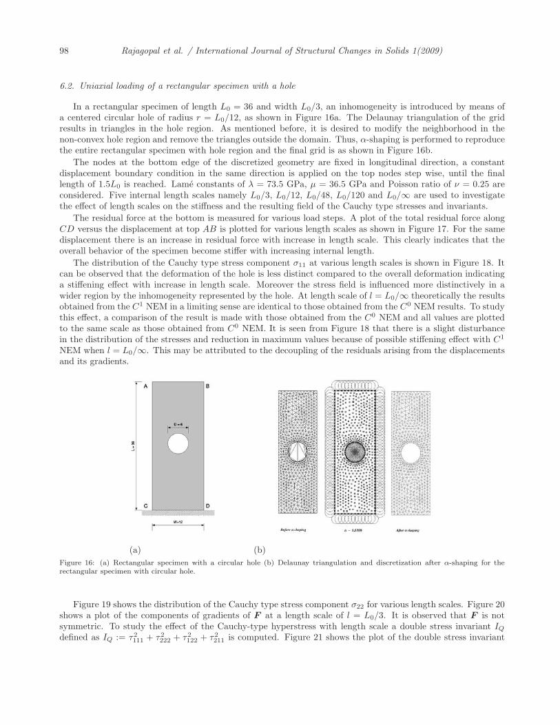
In a rectangular specimen of length L0 = 36 and width L0/3, an inhomogeneity is introduced by means ofa centered circular hole of radius r = L0/12, as shown in Figure 16a. The Delaunay triangulation of the gridresults in triangles in the hole region. As mentioned before, it is desired to modify the neighborhood in thenon-convex hole region and remove the triangles outside the domain. Thus, α-shaping is performed to reproducethe entire rectangular specimen with hole region and the final grid is as shown in Figure 16b.
The nodes at the bottom edge of the discretized geometry are fixed in longitudinal direction, a constantdisplacement boundary condition in the same direction is applied on the top nodes step wise, until the finallength of 1.5L0 is reached. Lame constants of λ = 73.5 GPa, μ = 36.5 GPa and Poisson ratio of ν = 0.25 areconsidered. Five internal length scales namely L0/3, L0/12, L0/48, L0/120 and L0/∞ are used to investigatethe effect of length scales on the stiffness and the resulting field of the Cauchy type stresses and invariants.
The residual force at the bottom is measured for various load steps. A plot of the total residual force alongCD versus the displacement at top AB is plotted for various length scales as shown in Figure 17. For the samedisplacement there is an increase in residual force with increase in length scale. This clearly indicates that theoverall behavior of the specimen become stiffer with increasing internal length.
The distribution of the Cauchy type stress component σ11 at various length scales is shown in Figure 18. Itcan be observed that the deformation of the hole is less distinct compared to the overall deformation indicatinga stiffening effect with increase in length scale. Moreover the stress field is influenced more distinctively in awider region by the inhomogeneity represented by the hole. At length scale of l = L0/∞ theoretically the resultsobtained from the C1 NEM in a limiting sense are identical to those obtained from the C0 NEM results. To studythis effect, a comparison of the result is made with those obtained from the C0 NEM and all values are plottedto the same scale as those obtained from C0 NEM. It is seen from Figure 18 that there is a slight disturbancein the distribution of the stresses and reduction in maximum values because of possible stiffening effect with C1
NEM when l = L0/∞. This may be attributed to the decoupling of the residuals arising from the displacementsand its gradients.
(a) (b)Figure 16: (a) Rectangular specimen with a circular hole (b) Delaunay triangulation and discretization after α-shaping for therectangular specimen with circular hole.
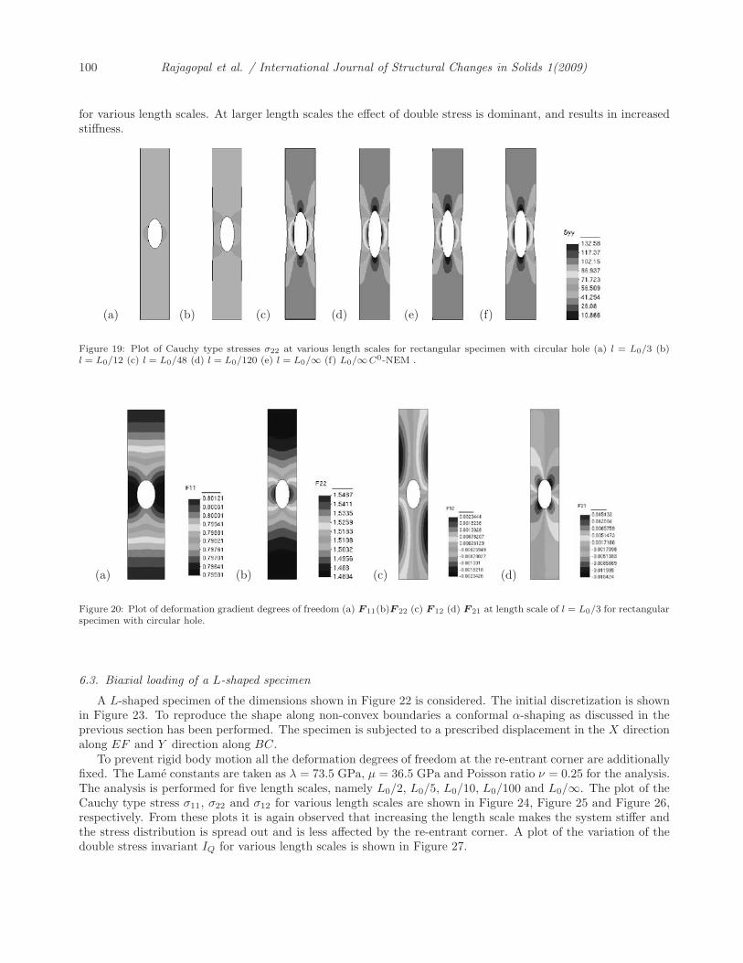
Figure 19 shows the distribution of the Cauchy type stress component σ22 for various length scales. Figure 20shows a plot of the components of gradients of F at a length scale of l = L0/3. It is observed that F is notsymmetric. To study the effect of the Cauchy-type hyperstress with length scale a double stress invariant IQdefined as IQ := τ2
111 + τ2222 + τ2
122 + τ2211 is computed. Figure 21 shows the plot of the double stress invariant
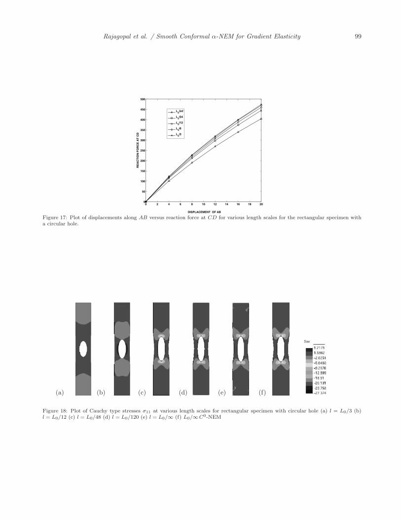
Rajagopal et al. / Smooth Conformal α-NEM for Gradient Elasticity 99
0 2 4 6 8 10 12 14 16 18 200
50
100
150
200
250
300
350
400
450
500
DISPLACEMENT OF AB
RE
AC
TIO
N F
OR
CE
AT
CD
L0/inf
L0/24
L0/12
L0/6
L0/3
Figure 17: Plot of displacements along AB versus reaction force at CD for various length scales for the rectangular specimen witha circular hole.
(a) (b) (c) (d) (e) (f)
Figure 18: Plot of Cauchy type stresses σ11 at various length scales for rectangular specimen with circular hole (a) l = L0/3 (b)l = L0/12 (c) l = L0/48 (d) l = L0/120 (e) l = L0/∞ (f) L0/∞C0-NEM
100 Rajagopal et al. / International Journal of Structural Changes in Solids 1(2009)
for various length scales. At larger length scales the effect of double stress is dominant, and results in increasedstiffness.
(a) (b) (c) (d) (e) (f)
Figure 19: Plot of Cauchy type stresses σ22 at various length scales for rectangular specimen with circular hole (a) l = L0/3 (b)l = L0/12 (c) l = L0/48 (d) l = L0/120 (e) l = L0/∞ (f) L0/∞C0-NEM .
(a) (b) (c) (d)
Figure 20: Plot of deformation gradient degrees of freedom (a) F11(b)F 22 (c) F 12 (d) F21 at length scale of l = L0/3 for rectangularspecimen with circular hole.
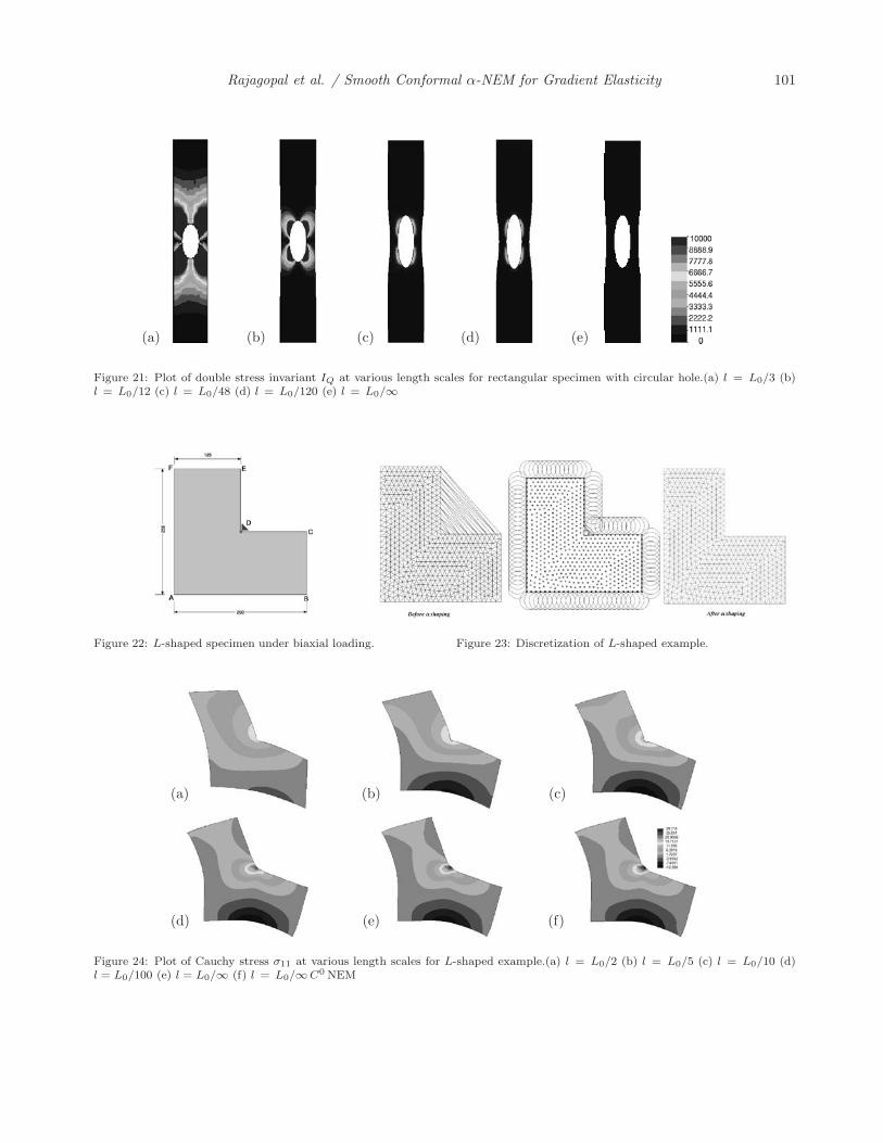
6.3. Biaxial loading of a L-shaped specimen
A L-shaped specimen of the dimensions shown in Figure 22 is considered. The initial discretization is shownin Figure 23. To reproduce the shape along non-convex boundaries a conformal α-shaping as discussed in theprevious section has been performed. The specimen is subjected to a prescribed displacement in the X directionalong EF and Y direction along BC.
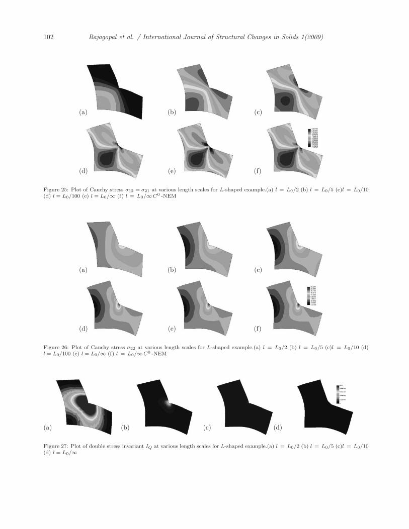
To prevent rigid body motion all the deformation degrees of freedom at the re-entrant corner are additionallyfixed. The Lame constants are taken as λ = 73.5 GPa, μ = 36.5 GPa and Poisson ratio ν = 0.25 for the analysis.The analysis is performed for five length scales, namely L0/2, L0/5, L0/10, L0/100 and L0/∞. The plot of theCauchy type stress σ11, σ22 and σ12 for various length scales are shown in Figure 24, Figure 25 and Figure 26,respectively. From these plots it is again observed that increasing the length scale makes the system stiffer andthe stress distribution is spread out and is less affected by the re-entrant corner. A plot of the variation of thedouble stress invariant IQ for various length scales is shown in Figure 27.
Rajagopal et al. / Smooth Conformal α-NEM for Gradient Elasticity 101
(a) (b) (c) (d) (e)
Figure 21: Plot of double stress invariant IQ at various length scales for rectangular specimen with circular hole.(a) l = L0/3 (b)l = L0/12 (c) l = L0/48 (d) l = L0/120 (e) l = L0/∞
Figure 22: L-shaped specimen under biaxial loading. Figure 23: Discretization of L-shaped example.
(a) (b) (c)
(d) (e) (f)
Figure 24: Plot of Cauchy stress σ11 at various length scales for L-shaped example.(a) l = L0/2 (b) l = L0/5 (c) l = L0/10 (d)l = L0/100 (e) l = L0/∞ (f) l = L0/∞C0 NEM
102 Rajagopal et al. / International Journal of Structural Changes in Solids 1(2009)
(a) (b) (c)
(d) (e) (f)
Figure 25: Plot of Cauchy stress σ12 = σ21 at various length scales for L-shaped example.(a) l = L0/2 (b) l = L0/5 (c)l = L0/10(d) l = L0/100 (e) l = L0/∞ (f) l = L0/∞C0 -NEM
(a) (b) (c)
(d) (e) (f)
Figure 26: Plot of Cauchy stress σ22 at various length scales for L-shaped example.(a) l = L0/2 (b) l = L0/5 (c)l = L0/10 (d)l = L0/100 (e) l = L0/∞ (f) l = L0/∞C0 -NEM
(a) (b) (c) (d)
Figure 27: Plot of double stress invariant IQ at various length scales for L-shaped example.(a) l = L0/2 (b) l = L0/5 (c)l = L0/10(d) l = L0/∞

Rajagopal et al. / Smooth Conformal α-NEM for Gradient Elasticity 103
Figure 28: Square block example. Figure 29: Discretization for the square block example.
6.4. Uniaxial compression of a square block
A square block of the dimensions shown in Figure 28 is subjected to a non-uniform compression. Displace-ments are applied along EF and GH so as to induce non uniform compression. It is desired to investigate theresulting Cauchy stress distribution at various length scales. Because of the symmetry only one-half of the blockis considered for convenience. The block is discretized as shown in Figure 29. Figure 30 shows the distributionof the Cauchy stress σ11 at various length scales. Figure 31 and Figure 32 display the distribution of the Cauchystress σ22 and σ12 at various length scales. Again the main feature to observe is that the overall behavior of thespecimen becomes stiffer with increasing internal length.
(a) (b) (c)
(d) (e) (f)
Figure 30: Plot of Cauchy stress σ11 at various length scales for the square block example. (a) l = L0/2 (b) l = L0/5 (c) l = L0/10(d) l = L0/100 (e) l = L0/∞ (f) l = L0/∞ (g) C0-NEM
6.5. Uniaxial loading of a cracked specimen
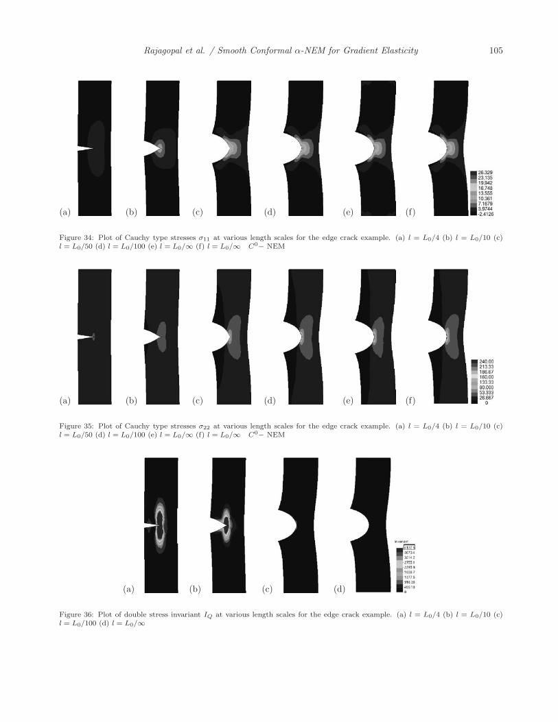
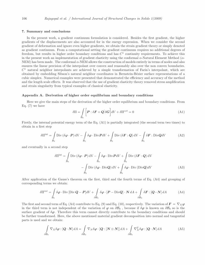
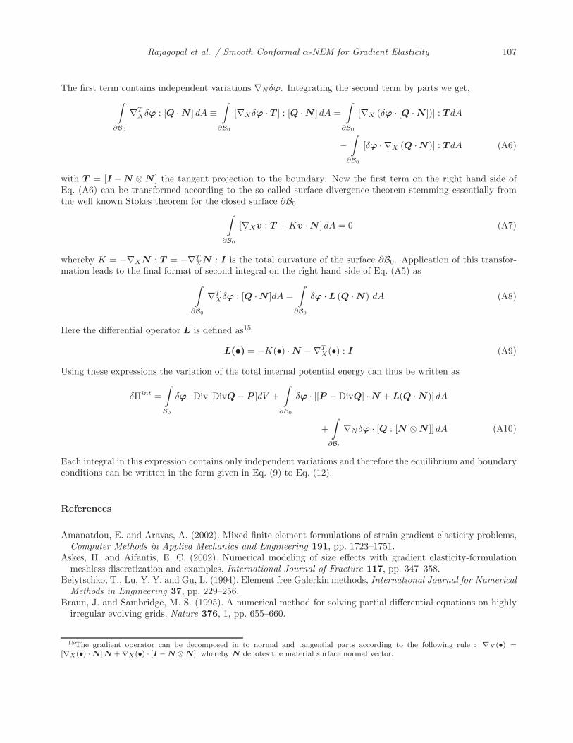
A rectangular specimen with an edge crack under uniaxial quasi-static loading is considered (see Figure 33a).The discretization is shown in Figure 33b. The displacements at the bottom edge AB is fixed and uniaxialdisplacement is applied at the top edge CD. The neighborhood at the crack edge is modified by imposing avisibility criterion as given in Sukumar et al. (1998). The influence of the variation of length scale on the Cauchytype stresses are studied. Five length scales L0/4, L0/10, L0/50, L0/100 and L0/∞ are considered for theanalysis. For the variation of the internal length the Cauchy type stress σ11 is plotted in Figure 34. Figure 35shows the distribution of the normal component of the Cauchy stress σ22 in the loading direction. A comparisonof the stresses at zero length scale is made with those obtained from C0 NEM. It is observed that the possibledecoupling between the residuals results in a slight disturbance of stresses obtained from C1 NEM. The doublestress invariants are shown in Figure 36. The plot indicates the increase in the stiffness with length scales.

104 Rajagopal et al. / International Journal of Structural Changes in Solids 1(2009)
(a) (b) (c)
(d) (e) (f)
Figure 31: Plot of Cauchy stress σ22 at various length scales for the square block example. (a) l = L0/2 (b) l = L0/5 (c) l = L0/10(d) l = L0/100 (e) l = L0/∞ (f) l = L0/∞ (g) C0-NEM
(a) (b) (c)
(d) (e) (f)
Figure 32: Plot of Cauchy stress σ12 = σ21 at various length scales for the square block example. (a) l = L0/2 (b) l = L0/5 (c)l = L0/10 (d) l = L0/100 (e) l = L0/∞ (f) l = L0/∞ (g) C0-NEM
(a) (b)
Figure 33: (a) Rectangular specimen with an edge crack. (b) Nodal discretization for the edge crack example.
Rajagopal et al. / Smooth Conformal α-NEM for Gradient Elasticity 105
(a) (b) (c) (d) (e) (f)
Figure 34: Plot of Cauchy type stresses σ11 at various length scales for the edge crack example. (a) l = L0/4 (b) l = L0/10 (c)l = L0/50 (d) l = L0/100 (e) l = L0/∞ (f) l = L0/∞ C0− NEM
(a) (b) (c) (d) (e) (f)
Figure 35: Plot of Cauchy type stresses σ22 at various length scales for the edge crack example. (a) l = L0/4 (b) l = L0/10 (c)l = L0/50 (d) l = L0/100 (e) l = L0/∞ (f) l = L0/∞ C0− NEM
(a) (b) (c) (d)
Figure 36: Plot of double stress invariant IQ at various length scales for the edge crack example. (a) l = L0/4 (b) l = L0/10 (c)l = L0/100 (d) l = L0/∞
106 Rajagopal et al. / International Journal of Structural Changes in Solids 1(2009)
7. Summary and conclusions
In the present work, a gradient continuum formulation is considered. Besides the first gradient, the highergradients of the displacements are also accounted for in the energy expression. When we consider the secondgradient of deformation and ignore even higher gradients, we obtain the strain gradient theory or simply denotedas gradient continuum. From a computational setting the gradient continuum requires no additional degrees offreedom, but results in higher order boundary conditions and has C1 continuity requirements. To achieve thisin the present work an implementation of gradient elasticity using the conformal α-Natural Element Method (α-NEM) has been made. The conformal α-NEM allows the construction of models entirely in terms of nodes and alsoensures the linear precision of the interpolant over convex and reasonably also over the non convex boundaries.C1 natural neighbor interpolants are achieved by a simple transformation of Farin’s interpolant, which areobtained by embedding Sibson’s natural neighbor coordinates in Bernstein-Bezier surface representations of acubic simplex. Numerical examples were presented that demonstrated the efficiency and accuracy of the methodand the length scale effects. It was observed that the use of gradient elasticity theory removed stress amplificationand strain singularity from typical examples of classical elasticity.
Appendix A. Derivation of higher order equilibrium and boundary conditions
Here we give the main steps of the derivation of the higher order equilibrium and boundary conditions. FromEq. (7) we have
δΠ =∫B0
[P : δF + Q
...δG]dV + δΠext = 0 (A1)
Firstly, the internal potential energy term of the Eq. (A1) is partially integrated (the second term two times) toobtain in a first step
δΠint =∫B0
Div (δϕ · P ) dV −∫B0
δϕ · DivP dV +∫B0
Div (δF : Q) dV −∫B0
δF : DivQdV (A2)
and eventually in a second step
δΠint =∫B0
Div (δϕ · P ) dV −∫B0
δϕ · DivP dV +∫B0
Div (δF : Q) dV
−∫B0
Div (δϕ · DivQ) dV +∫B0
δϕ · Div (DivQ)dV (A3)
After application of the Gauss’s theorem on the first, third and the fourth terms of Eq. (A4) and grouping ofcorresponding terms we obtain:
δΠint =∫B0
δϕ · Div [Div Q − P ]dV +∫
∂B0
δϕ · [P − DivQ] · N dA+∫
∂B0
δF : [Q · N ] dA (A4)
The first and second term of Eq. (A4) contribute to Eq. (9) and Eq. (10), respectively. The variation of F = ∇Xϕin the third term is not independent of the variation of ϕ on ∂B0 , because if δϕ is known on ∂B0 so is thesurface gradient of δϕ. Therefore this term cannot directly contribute to the boundary conditions and shouldbe further transformed. Here, the above mentioned material gradient decomposition into normal and tangentialparts is used and we obtain:∫
∂B0
∇Xδϕ : [Q · N ] dA =∫
∂B0
∇N δϕ · [Q : [N ⊗ N ]] dA+∫
∂B0
∇TXδϕ : [Q · N ] dA (A5)
Rajagopal et al. / Smooth Conformal α-NEM for Gradient Elasticity 107
The first term contains independent variations ∇Nδϕ. Integrating the second term by parts we get,∫∂B0
∇TXδϕ : [Q · N ] dA ≡
∫∂B0
[∇Xδϕ · T ] : [Q · N ]dA =∫
∂B0
[∇X (δϕ · [Q · N ])] : T dA
−∫
∂B0
[δϕ · ∇X (Q · N )] : T dA (A6)
with T = [I − N ⊗ N ] the tangent projection to the boundary. Now the first term on the right hand side ofEq. (A6) can be transformed according to the so called surface divergence theorem stemming essentially fromthe well known Stokes theorem for the closed surface ∂B0∫
∂B0
[∇Xv : T +Kv · N ] dA = 0 (A7)
whereby K = −∇XN : T = −∇TXN : I is the total curvature of the surface ∂B0. Application of this transfor-
mation leads to the final format of second integral on the right hand side of Eq. (A5) as∫∂B0
∇TXδϕ : [Q · N ]dA =
∫∂B0
δϕ · L (Q · N) dA (A8)
Here the differential operator L is defined as15
L(•) = −K(•) · N −∇TX(•) : I (A9)
Using these expressions the variation of the total internal potential energy can thus be written as
δΠint =∫B0
δϕ · Div [DivQ − P ]dV +∫
∂B0
δϕ · [[P − DivQ] · N + L(Q · N)] dA
+∫
∂B′
∇N δϕ · [Q : [N ⊗ N ]] dA (A10)
Each integral in this expression contains only independent variations and therefore the equilibrium and boundaryconditions can be written in the form given in Eq. (9) to Eq. (12).
References
Amanatdou, E. and Aravas, A. (2002). Mixed finite element formulations of strain-gradient elasticity problems,Computer Methods in Applied Mechanics and Engineering 191, pp. 1723–1751.
Askes, H. and Aifantis, E. C. (2002). Numerical modeling of size effects with gradient elasticity-formulationmeshless discretization and examples, International Journal of Fracture 117, pp. 347–358.
Belytschko, T., Lu, Y. Y. and Gu, L. (1994). Element free Galerkin methods, International Journal for NumericalMethods in Engineering 37, pp. 229–256.
Braun, J. and Sambridge, M. S. (1995). A numerical method for solving partial differential equations on highlyirregular evolving grids, Nature 376, 1, pp. 655–660.
15The gradient operator can be decomposed in to normal and tangential parts according to the following rule : ∇X(•) =[∇X(•) · N] N + ∇X(•) · [I − N ⊗ N], whereby N denotes the material surface normal vector.
108 Rajagopal et al. / International Journal of Structural Changes in Solids 1(2009)
Cazals, F., Giesen, J., Pauly, M. and Zomorodian, A. (2006). The conformal alpha shape filtration, VisualComputations 22, pp. 531–540.
Cueto, E., Doblare, M. and Calvo, B. (2002). Modelling three dimensional piece wise homogeneous domains usingthe α-shape based natural element method, International Journal for Numerical Methods in Engineering 54,pp. 871–897.
Cueto, E., Doblare, M. and Gracia, L. (2000). Imposing essential boundary conditions in the natural elementmethod by means of density scaled α-shapes, International Journal for Numerical Methods in Engineering 49,pp. 519–546.
Edelsbrunner, H., Kirkpatrick, D. and Seidel, R. (1983). On the shape of a set of points in plane, IEEE Trans-actions on information theory. 29, 4, pp. 551–559.
Edelsbrunner, H. and Mucke, E. (1994). Three dimensional alpha shapes, ACM transactions on graphics 13, 1,pp. 43–72.
Eringen, A. C. (1964). Mechanics of micromorphic materials, in H. Gorliter (ed.), Proc. 11th Int. Congress ofAppl. Mech., pp. 131–138.
Eringen, A. C. (1970). Balance laws of micromorphic mechanics, International Journal of Engineering Science85, pp. 819–828.
Eringen, A. C. (1992). Balance laws of micromorphic continuua revisited, International Journal of EngineeringScience 30, 6, pp. 805–810.
Eringen, A. C. (1998). Microcontinuum field theories-1. foundations and solids, Springer-Verlag, Newyork, Inc. .Farin, R. (1985). Curves and surfaces for computer aided geometric design, Computer science and Scientific
computing, Academic press,London , UK 4th edition, pp. 19–27.Farin, R. (1986). Triangular Bernstein Bezier patches, Computer Aided Geometirc Design 7, pp. 83–127.Farin, R. (1990). Surfaces over Dirichlet tesellations, Computer Aided Geometric Design 7, pp. 281–292.Fleck, N. and Hutchinson, J. (1996). Strain gradient plasticity, Adv. app.Mech 33.Hirschberger, B. and Steinmann, P. (2007). On deformation and configurational mechanics of micromorphic
hyperelasticity-theory and computations, Computer Methods in Applied Mechanics and Engineering 40, 4,pp. 4027 – 4044.
Kirchner, N. and Steinmann, P. (2005). A unifying treatise on variational principles of gradient and micromorphiccontinuaa, Philosophical Magazine 85, 33-35, pp. 3875–3895.
Kirchner, N. and Steinmann, P. (2007). On material setting of gradient hyperelasticity, Mathematics and Me-chanics of Solids 12, 5, pp. 559–580.
Kouznetsova, V. G. (2002). Computational homogenization for the multiscale analysis of multipahse materials,PhD, thesis, Technische Universiteit, Eindhoven .
Kouznetsova, V. G., Geers, M. G. D. and Brekelmans, W. A. M. (2004). Multiscale second order computationalhomogenization of multiphase materials: A nested finite element solution strategy, Computer Methods inApplied Mechanics and Engineering 193, pp. 5525–5550.
Mindlin, D. and Tiersten, H. F. (1962). Effects of couple stress in linear elasticity, Arc. Rat. Mech. Anal. 11, pp.415–448.
Mindlin, D. and Tiersten, H. F. (1964). Microstructure in linear elasticity, Arc. Rat. Mech. Anal. 16, pp. 51–78.Mindlin, R. D. (1965). Second gradient in strain and surface tension in linear elasticity, Int. J. of Solids and
Structures 1, 3, pp. 417–438.Sambridge, M. S., Braun, J. and McQueen, H. (1995). Geophysical parametrization and interpolation of irregular
data using natural neighbours, Geophys. J. Int. 122, 1, pp. 837–857.Shu, J., King, W. and Fleck, N. (1999). Finite elements for materials with strain gradient effects, International
Journal for Numerical Methods in Engineering 44, pp. 373–391.Sibson, R. (1980). A vector identity for the Dirichlet tessellation, Mathematical Proceedings of Cambridge Philo-
sophical Society 87, pp. 151–155.Sibson, R. (1981). A brief description of natural neighbor interpolation, in V. Barnett (ed.), Interpreting Multi-
variate Data (John Wiley, Chichester), pp. 21–36.Stogner, R. H. and Carey, G. F. (2007). C1 macro elements in adaptive finite element methods, International
Journal of numerical methods in engineering 70, pp. 1076–1095.
Rajagopal et al. / Smooth Conformal α-NEM for Gradient Elasticity 109
Sukumar, N. and Moran, B. (1999). C1 natural neighbour interpolant for partial differential equations, Interna-tional Journal for Numerical Methods in Engineering 15, 1, pp. 417–447.
Sukumar, N., Moran, B. and Belytschko, T. (1998). The natural element method in solid mechanics, InternationalJournal for Numerical Methods in Engineering 43, 1, pp. 839–887.
Sunyk, R. and Steinmann, P. (2003). On higher gradients in continuum atomistic modelling, International Journalof Solids and Structures 40, pp. 6877–6896.
Tang, Z., Shen, S. and Atluri, S. N. (2003). Analysis of materials with strain gradient effects: A mesh less localpetrov Galerkin approach, with nodal displacements only, Computer modelling in Engineering Sciences 4, 1,pp. 177–196.
Toupin, R. A. (1962). Elastic materials with couple stress, Arc. Rat. Mech. Anal. 11, pp. 385–414.


![DiversityOriented Synthesis of Lactams and Lactams by ... · ment of diversity-oriented syntheses of various heterocyclic scaffolds through post-Ugi transformations,[15] we envi-sioned](https://static.fdocument.org/doc/165x107/5f26bb4b96f4525a733541e9/diversityoriented-synthesis-of-lactams-and-lactams-by-ment-of-diversity-oriented.jpg)