The Not So ShortIntroduction to LATEX2ε

Or LATEX 2ε in 139 minutes

by Tobias Oetiker

Hubert Partl, Irene Hyna and Elisabeth Schlegl

Version 4.24, February 08, 2008

ii

Copyright ©1995-2005 Tobias Oetiker and Contributers. All rights reserved.This document is free; you can redistribute it and/or modify it under the terms

of the GNU General Public License as published by the Free Software Foundation;either version 2 of the License, or (at your option) any later version.

This document is distributed in the hope that it will be useful, but WITHOUTANY WARRANTY; without even the implied warranty of MERCHANTABILITYor FITNESS FOR A PARTICULAR PURPOSE. See the GNU General PublicLicense for more details.

You should have received a copy of the GNU General Public License along withthis document; if not, write to the Free Software Foundation, Inc., 675 Mass Ave,Cambridge, MA 02139, USA.

Thank you!

Much of the material used in this introduction comes from an Austrianintroduction to LATEX 2.09 written in German by:

Hubert Partl <partl@mail.boku.ac.at>Zentraler Informatikdienst der Universität für Bodenkultur Wien

Irene Hyna <Irene.Hyna@bmwf.ac.at>Bundesministerium für Wissenschaft und Forschung Wien

Elisabeth Schlegl <noemail>in Graz

If you are interested in the German document, you can find a versionupdated for LATEX2ε by Jörg Knappen atCTAN:/tex-archive/info/lshort/german

iv Thank you!

The following individuals helped with corrections, suggestions and materialto improve this paper. They put in a big effort to help me get this documentinto its present shape. I would like to sincerely thank all of them. Naturally,all the mistakes you’ll find in this book are mine. If you ever find a wordthat is spelled correctly, it must have been one of the people below droppingme a line.

Rosemary Bailey, Marc Bevand, Friedemann Brauer, Barbara Beeton, Jan Busa,Markus Brühwiler, Pietro Braione, David Carlisle, José Carlos Santos,Neil Carter, Mike Chapman, Pierre Chardaire, Christopher Chin, Carl Cerecke,Chris McCormack, Wim van Dam, Jan Dittberner, Michael John Downes,Matthias Dreier, David Dureisseix, Elliot, Hans Ehrbar, Daniel Flipo, David Frey,Hans Fugal, Robin Fairbairns, Jörg Fischer, Erik Frisk, Mic Milic Frederickx,Frank, Kasper B. Graversen, Arlo Griffiths, Alexandre Guimond, Andy Goth,Cyril Goutte, Greg Gamble, Frank Fischli, Morten Høgholm, Neil Hammond,Rasmus Borup Hansen, Joseph Hilferty, Björn Hvittfeldt, Martien Hulsen,Werner Icking, Jakob, Eric Jacoboni, Alan Jeffrey, Byron Jones, David Jones,Johannes-Maria Kaltenbach, Michael Koundouros, Andrzej Kawalec,Sander de Kievit, Alain Kessi, Christian Kern, Tobias Klauser, Jörg Knappen,Kjetil Kjernsmo, Maik Lehradt, Rémi Letot, Flori Lambrechts, Axel Liljencrantz,Johan Lundberg, Alexander Mai, Hendrik Maryns, Martin Maechler,Aleksandar S Milosevic, Henrik Mitsch, Claus Malten, Kevin Van Maren,Richard Nagy, Philipp Nagele, Lenimar Nunes de Andrade, Manuel Oetiker,Urs Oswald, Lan Thuy Pham, Martin Pfister, Demerson Andre Polli,Nikos Pothitos, Maksym Polyakov Hubert Partl, John Refling, Mike Ressler,Brian Ripley, Young U. Ryu, Bernd Rosenlecher, Kurt Rosenfeld, Chris Rowley,Risto Saarelma, Hanspeter Schmid, Craig Schlenter, Gilles Schintgen,Baron Schwartz, Christopher Sawtell, Miles Spielberg, Geoffrey Swindale,Laszlo Szathmary, Boris Tobotras, Josef Tkadlec, Scott Veirs, Didier Verna,Fabian Wernli, Carl-Gustav Werner, David Woodhouse, Chris York,Fritz Zaucker, Rick Zaccone, and Mikhail Zotov.

Preface

LATEX [1] is a typesetting system that is very suitable for producing scien-tific and mathematical documents of high typographical quality. It is alsosuitable for producing all sorts of other documents, from simple letters tocomplete books. LATEX uses TEX [2] as its formatting engine.

This short introduction describes LATEX2ε and should be sufficient formost applications of LATEX. Refer to [1, 3] for a complete description of theLATEX system.

This introduction is split into 6 chapters:

Chapter 1 tells you about the basic structure of LATEX2ε documents. Youwill also learn a bit about the history of LATEX. After reading thischapter, you should have a rough understanding how LATEX works.

Chapter 2 goes into the details of typesetting your documents. It explainsmost of the essential LATEX commands and environments. After read-ing this chapter, you will be able to write your first documents.

Chapter 3 explains how to typeset formulae with LATEX. Many examplesdemonstrate how to use one of LATEX’s main strengths. At the endof the chapter are tables listing all mathematical symbols available inLATEX.

Chapter 4 explains indexes, bibliography generation and inclusion of EPSgraphics. It introduces creation of PDF documents with pdfLATEX andpresents some handy extension packages.

Chapter 5 shows how to use LATEX for creating graphics. Instead of draw-ing a picture with some graphics program, saving it to a file and thenincluding it into LATEX you describe the picture and have LATEX drawit for you.

Chapter 6 contains some potentially dangerous information about how toalter the standard document layout produced by LATEX. It will tell youhow to change things such that the beautiful output of LATEX turnsugly or stunning, depending on your abilities.

vi Preface

It is important to read the chapters in order—the book is not that big, afterall. Be sure to carefully read the examples, because a lot of the informationis in the examples placed throughout the book.

LATEX is available for most computers, from the PC and Mac to large UNIXand VMS systems. On many university computer clusters you will find thata LATEX installation is available, ready to use. Information on how to accessthe local LATEX installation should be provided in the Local Guide [5]. If youhave problems getting started, ask the person who gave you this booklet.The scope of this document is not to tell you how to install and set up aLATEX system, but to teach you how to write your documents so that theycan be processed by LATEX.

If you need to get hold of any LATEX related material, have a look at oneof the Comprehensive TEX Archive Network (CTAN) sites. The homepage isat http://www.ctan.org. All packages can also be retrieved from the ftparchive ftp://www.ctan.org and its mirror sites all over the world.

You will find other references to CTAN throughout the book, especiallypointers to software and documents you might want to download. Insteadof writing down complete urls, I just wrote CTAN: followed by whateverlocation within the CTAN tree you should go to.

If you want to run LATEX on your own computer, take a look at what isavailable from CTAN:/tex-archive/systems.

If you have ideas for something to be added, removed or altered in thisdocument, please let me know. I am especially interested in feedback fromLATEX novices about which bits of this intro are easy to understand andwhich could be explained better.

Tobias Oetiker <tobi@oetiker.ch>

OETIKER+PARTNER AGAarweg 154600 OltenSwitzerland

The current version of this document is available onCTAN:/tex-archive/info/lshort

Contents

Thank you! iii

Preface v

1 Things You Need to Know 11.1 The Name of the Game . . . . . . . . . . . . . . . . . . . . . 1

1.1.1 TEX . . . . . . . . . . . . . . . . . . . . . . . . . . . . 11.1.2 LATEX . . . . . . . . . . . . . . . . . . . . . . . . . . . 2

1.2 Basics . . . . . . . . . . . . . . . . . . . . . . . . . . . . . . . 21.2.1 Author, Book Designer, and Typesetter . . . . . . . . 21.2.2 Layout Design . . . . . . . . . . . . . . . . . . . . . . 21.2.3 Advantages and Disadvantages . . . . . . . . . . . . . 3

1.3 LATEX Input Files . . . . . . . . . . . . . . . . . . . . . . . . . 41.3.1 Spaces . . . . . . . . . . . . . . . . . . . . . . . . . . . 41.3.2 Special Characters . . . . . . . . . . . . . . . . . . . . 51.3.3 LATEX Commands . . . . . . . . . . . . . . . . . . . . 51.3.4 Comments . . . . . . . . . . . . . . . . . . . . . . . . . 6

1.4 Input File Structure . . . . . . . . . . . . . . . . . . . . . . . 71.5 A Typical Command Line Session . . . . . . . . . . . . . . . 71.6 The Layout of the Document . . . . . . . . . . . . . . . . . . 9

1.6.1 Document Classes . . . . . . . . . . . . . . . . . . . . 91.6.2 Packages . . . . . . . . . . . . . . . . . . . . . . . . . 101.6.3 Page Styles . . . . . . . . . . . . . . . . . . . . . . . . 13

1.7 Files You Might Encounter . . . . . . . . . . . . . . . . . . . 131.8 Big Projects . . . . . . . . . . . . . . . . . . . . . . . . . . . . 14

2 Typesetting Text 172.1 The Structure of Text and Language . . . . . . . . . . . . . . 172.2 Line Breaking and Page Breaking . . . . . . . . . . . . . . . . 19

2.2.1 Justified Paragraphs . . . . . . . . . . . . . . . . . . . 192.2.2 Hyphenation . . . . . . . . . . . . . . . . . . . . . . . 20

2.3 Ready-Made Strings . . . . . . . . . . . . . . . . . . . . . . . 212.4 Special Characters and Symbols . . . . . . . . . . . . . . . . . 21

viii CONTENTS

2.4.1 Quotation Marks . . . . . . . . . . . . . . . . . . . . . 212.4.2 Dashes and Hyphens . . . . . . . . . . . . . . . . . . . 222.4.3 Tilde (∼) . . . . . . . . . . . . . . . . . . . . . . . . . 222.4.4 Degree Symbol () . . . . . . . . . . . . . . . . . . . . 222.4.5 The Euro Currency Symbol (e) . . . . . . . . . . . . . 232.4.6 Ellipsis (. . . ) . . . . . . . . . . . . . . . . . . . . . . . 232.4.7 Ligatures . . . . . . . . . . . . . . . . . . . . . . . . . 242.4.8 Accents and Special Characters . . . . . . . . . . . . . 24

2.5 International Language Support . . . . . . . . . . . . . . . . . 252.5.1 Support for Portuguese . . . . . . . . . . . . . . . . . 272.5.2 Support for French . . . . . . . . . . . . . . . . . . . . 282.5.3 Support for German . . . . . . . . . . . . . . . . . . . 292.5.4 Support for Korean . . . . . . . . . . . . . . . . . . . . 292.5.5 Writing in Greek . . . . . . . . . . . . . . . . . . . . . 322.5.6 Support for Cyrillic . . . . . . . . . . . . . . . . . . . 33

2.6 The Space Between Words . . . . . . . . . . . . . . . . . . . . 332.7 Titles, Chapters, and Sections . . . . . . . . . . . . . . . . . . 352.8 Cross References . . . . . . . . . . . . . . . . . . . . . . . . . 372.9 Footnotes . . . . . . . . . . . . . . . . . . . . . . . . . . . . . 372.10 Emphasized Words . . . . . . . . . . . . . . . . . . . . . . . . 382.11 Environments . . . . . . . . . . . . . . . . . . . . . . . . . . . 38

2.11.1 Itemize, Enumerate, and Description . . . . . . . . . . 392.11.2 Flushleft, Flushright, and Center . . . . . . . . . . . . 392.11.3 Quote, Quotation, and Verse . . . . . . . . . . . . . . 402.11.4 Abstract . . . . . . . . . . . . . . . . . . . . . . . . . . 402.11.5 Printing Verbatim . . . . . . . . . . . . . . . . . . . . 412.11.6 Tabular . . . . . . . . . . . . . . . . . . . . . . . . . . 41

2.12 Floating Bodies . . . . . . . . . . . . . . . . . . . . . . . . . . 442.13 Protecting Fragile Commands . . . . . . . . . . . . . . . . . . 46

3 Typesetting Mathematical Formulae 493.1 The AMS-LATEX bundle . . . . . . . . . . . . . . . . . . . . . 493.2 Single Equations . . . . . . . . . . . . . . . . . . . . . . . . . 49

3.2.1 Math Mode . . . . . . . . . . . . . . . . . . . . . . . . 513.3 Building Blocks of a Mathematical Formula . . . . . . . . . . 523.4 Vertically Aligned Material . . . . . . . . . . . . . . . . . . . 57

3.4.1 Multiple Equations . . . . . . . . . . . . . . . . . . . . 573.4.2 Arrays and Matrices . . . . . . . . . . . . . . . . . . . 57

3.5 Spacing in Math Mode . . . . . . . . . . . . . . . . . . . . . . 583.5.1 Phantoms . . . . . . . . . . . . . . . . . . . . . . . . . 59

3.6 Fiddling with the Math Fonts . . . . . . . . . . . . . . . . . . 603.6.1 Bold Symbols . . . . . . . . . . . . . . . . . . . . . . . 60

3.7 Theorems, Lemmas, . . . . . . . . . . . . . . . . . . . . . . . . 613.8 List of Mathematical Symbols . . . . . . . . . . . . . . . . . . 63

CONTENTS ix

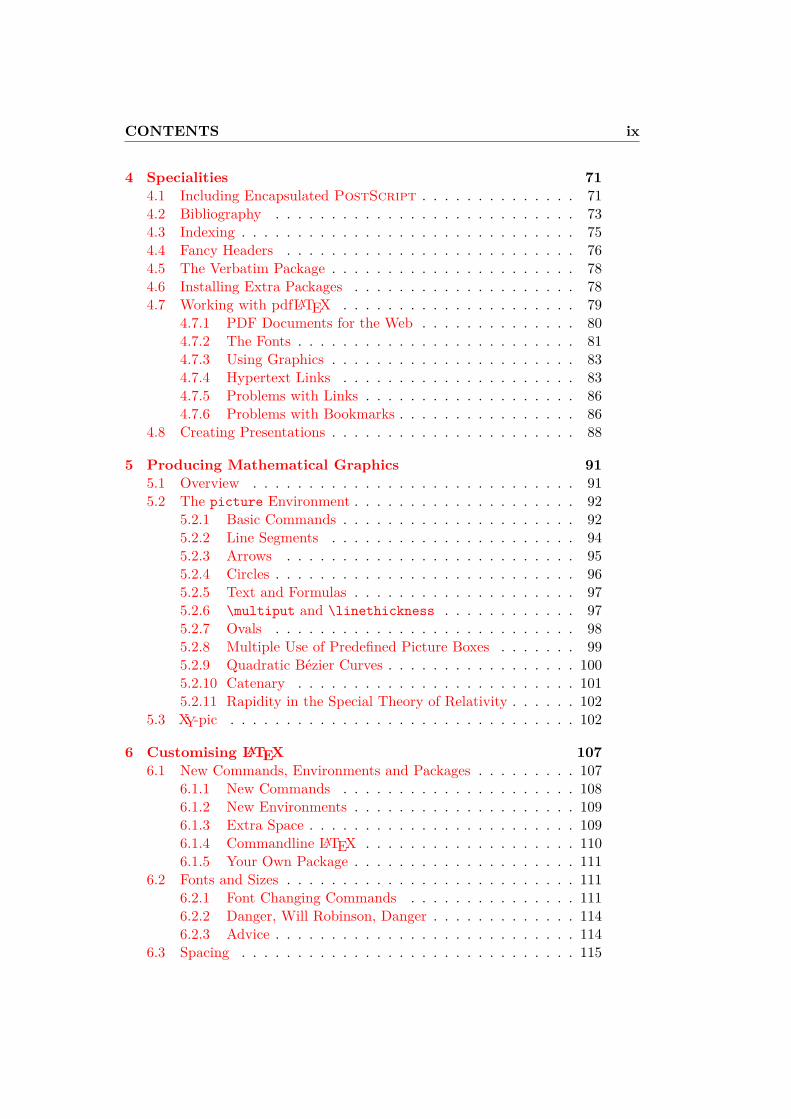
4 Specialities 714.1 Including Encapsulated PostScript . . . . . . . . . . . . . . 714.2 Bibliography . . . . . . . . . . . . . . . . . . . . . . . . . . . 734.3 Indexing . . . . . . . . . . . . . . . . . . . . . . . . . . . . . . 754.4 Fancy Headers . . . . . . . . . . . . . . . . . . . . . . . . . . 764.5 The Verbatim Package . . . . . . . . . . . . . . . . . . . . . . 784.6 Installing Extra Packages . . . . . . . . . . . . . . . . . . . . 784.7 Working with pdfLATEX . . . . . . . . . . . . . . . . . . . . . 79

4.7.1 PDF Documents for the Web . . . . . . . . . . . . . . 804.7.2 The Fonts . . . . . . . . . . . . . . . . . . . . . . . . . 814.7.3 Using Graphics . . . . . . . . . . . . . . . . . . . . . . 834.7.4 Hypertext Links . . . . . . . . . . . . . . . . . . . . . 834.7.5 Problems with Links . . . . . . . . . . . . . . . . . . . 864.7.6 Problems with Bookmarks . . . . . . . . . . . . . . . . 86

4.8 Creating Presentations . . . . . . . . . . . . . . . . . . . . . . 88

5 Producing Mathematical Graphics 915.1 Overview . . . . . . . . . . . . . . . . . . . . . . . . . . . . . 915.2 The picture Environment . . . . . . . . . . . . . . . . . . . . 92

5.2.1 Basic Commands . . . . . . . . . . . . . . . . . . . . . 925.2.2 Line Segments . . . . . . . . . . . . . . . . . . . . . . 945.2.3 Arrows . . . . . . . . . . . . . . . . . . . . . . . . . . 955.2.4 Circles . . . . . . . . . . . . . . . . . . . . . . . . . . . 965.2.5 Text and Formulas . . . . . . . . . . . . . . . . . . . . 975.2.6 \multiput and \linethickness . . . . . . . . . . . . 975.2.7 Ovals . . . . . . . . . . . . . . . . . . . . . . . . . . . 985.2.8 Multiple Use of Predefined Picture Boxes . . . . . . . 995.2.9 Quadratic Bézier Curves . . . . . . . . . . . . . . . . . 1005.2.10 Catenary . . . . . . . . . . . . . . . . . . . . . . . . . 1015.2.11 Rapidity in the Special Theory of Relativity . . . . . . 102

5.3 XY-pic . . . . . . . . . . . . . . . . . . . . . . . . . . . . . . . 102

6 Customising LATEX 1076.1 New Commands, Environments and Packages . . . . . . . . . 107

6.1.1 New Commands . . . . . . . . . . . . . . . . . . . . . 1086.1.2 New Environments . . . . . . . . . . . . . . . . . . . . 1096.1.3 Extra Space . . . . . . . . . . . . . . . . . . . . . . . . 1096.1.4 Commandline LATEX . . . . . . . . . . . . . . . . . . . 1106.1.5 Your Own Package . . . . . . . . . . . . . . . . . . . . 111

6.2 Fonts and Sizes . . . . . . . . . . . . . . . . . . . . . . . . . . 1116.2.1 Font Changing Commands . . . . . . . . . . . . . . . 1116.2.2 Danger, Will Robinson, Danger . . . . . . . . . . . . . 1146.2.3 Advice . . . . . . . . . . . . . . . . . . . . . . . . . . . 114

6.3 Spacing . . . . . . . . . . . . . . . . . . . . . . . . . . . . . . 115

x CONTENTS

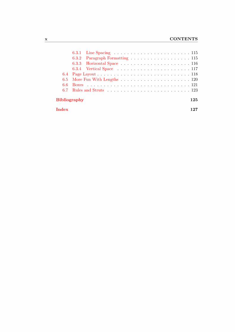
6.3.1 Line Spacing . . . . . . . . . . . . . . . . . . . . . . . 1156.3.2 Paragraph Formatting . . . . . . . . . . . . . . . . . . 1156.3.3 Horizontal Space . . . . . . . . . . . . . . . . . . . . . 1166.3.4 Vertical Space . . . . . . . . . . . . . . . . . . . . . . 117

6.4 Page Layout . . . . . . . . . . . . . . . . . . . . . . . . . . . . 1186.5 More Fun With Lengths . . . . . . . . . . . . . . . . . . . . . 1206.6 Boxes . . . . . . . . . . . . . . . . . . . . . . . . . . . . . . . 1216.7 Rules and Struts . . . . . . . . . . . . . . . . . . . . . . . . . 123

Bibliography 125

Index 127

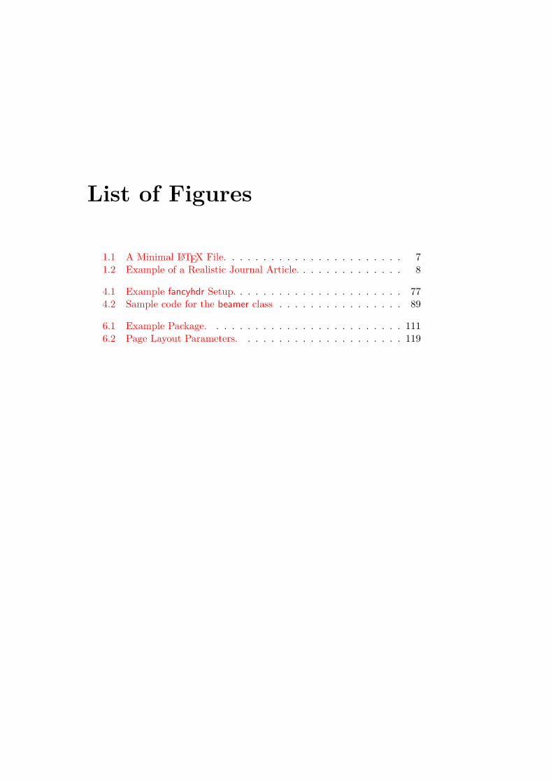
List of Figures

1.1 A Minimal LATEX File. . . . . . . . . . . . . . . . . . . . . . . 71.2 Example of a Realistic Journal Article. . . . . . . . . . . . . . 8

4.1 Example fancyhdr Setup. . . . . . . . . . . . . . . . . . . . . . 774.2 Sample code for the beamer class . . . . . . . . . . . . . . . . 89

6.1 Example Package. . . . . . . . . . . . . . . . . . . . . . . . . 1116.2 Page Layout Parameters. . . . . . . . . . . . . . . . . . . . . 119

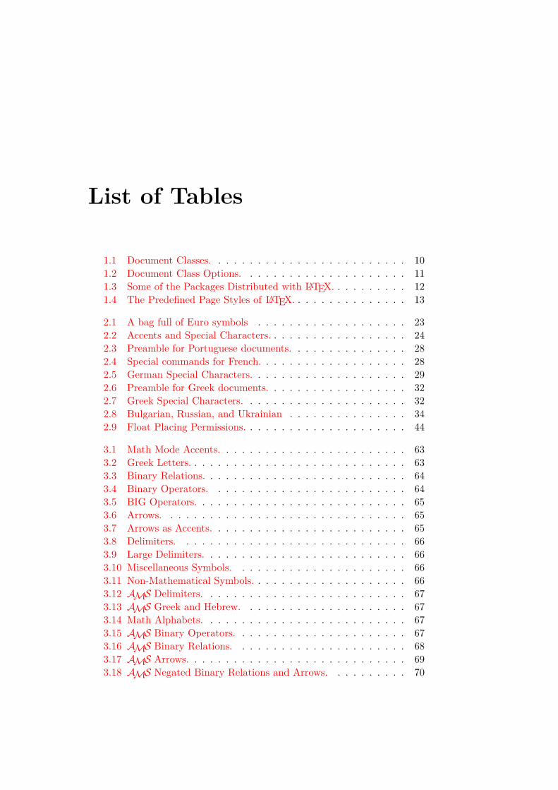
List of Tables

1.1 Document Classes. . . . . . . . . . . . . . . . . . . . . . . . . 101.2 Document Class Options. . . . . . . . . . . . . . . . . . . . . 111.3 Some of the Packages Distributed with LATEX. . . . . . . . . . 121.4 The Predefined Page Styles of LATEX. . . . . . . . . . . . . . . 13

2.1 A bag full of Euro symbols . . . . . . . . . . . . . . . . . . . 232.2 Accents and Special Characters. . . . . . . . . . . . . . . . . . 242.3 Preamble for Portuguese documents. . . . . . . . . . . . . . . 282.4 Special commands for French. . . . . . . . . . . . . . . . . . . 282.5 German Special Characters. . . . . . . . . . . . . . . . . . . . 292.6 Preamble for Greek documents. . . . . . . . . . . . . . . . . . 322.7 Greek Special Characters. . . . . . . . . . . . . . . . . . . . . 322.8 Bulgarian, Russian, and Ukrainian . . . . . . . . . . . . . . . 342.9 Float Placing Permissions. . . . . . . . . . . . . . . . . . . . . 44

3.1 Math Mode Accents. . . . . . . . . . . . . . . . . . . . . . . . 633.2 Greek Letters. . . . . . . . . . . . . . . . . . . . . . . . . . . . 633.3 Binary Relations. . . . . . . . . . . . . . . . . . . . . . . . . . 643.4 Binary Operators. . . . . . . . . . . . . . . . . . . . . . . . . 643.5 BIG Operators. . . . . . . . . . . . . . . . . . . . . . . . . . . 653.6 Arrows. . . . . . . . . . . . . . . . . . . . . . . . . . . . . . . 653.7 Arrows as Accents. . . . . . . . . . . . . . . . . . . . . . . . . 653.8 Delimiters. . . . . . . . . . . . . . . . . . . . . . . . . . . . . 663.9 Large Delimiters. . . . . . . . . . . . . . . . . . . . . . . . . . 663.10 Miscellaneous Symbols. . . . . . . . . . . . . . . . . . . . . . 663.11 Non-Mathematical Symbols. . . . . . . . . . . . . . . . . . . . 663.12 AMS Delimiters. . . . . . . . . . . . . . . . . . . . . . . . . . 673.13 AMS Greek and Hebrew. . . . . . . . . . . . . . . . . . . . . 673.14 Math Alphabets. . . . . . . . . . . . . . . . . . . . . . . . . . 673.15 AMS Binary Operators. . . . . . . . . . . . . . . . . . . . . . 673.16 AMS Binary Relations. . . . . . . . . . . . . . . . . . . . . . 683.17 AMS Arrows. . . . . . . . . . . . . . . . . . . . . . . . . . . . 693.18 AMS Negated Binary Relations and Arrows. . . . . . . . . . 70

xiv LIST OF TABLES

3.19 AMS Miscellaneous. . . . . . . . . . . . . . . . . . . . . . . . 70

4.1 Key Names for graphicx Package. . . . . . . . . . . . . . . . . 724.2 Index Key Syntax Examples. . . . . . . . . . . . . . . . . . . 75

6.1 Fonts. . . . . . . . . . . . . . . . . . . . . . . . . . . . . . . . 1126.2 Font Sizes. . . . . . . . . . . . . . . . . . . . . . . . . . . . . . 1126.3 Absolute Point Sizes in Standard Classes. . . . . . . . . . . . 1136.4 Math Fonts. . . . . . . . . . . . . . . . . . . . . . . . . . . . . 1136.5 TEX Units. . . . . . . . . . . . . . . . . . . . . . . . . . . . . 117

Chapter 1

Things You Need to Know

The first part of this chapter presents a short overview of the philosophy andhistory of LATEX2ε. The second part focuses on the basic structures of a LATEXdocument. After reading this chapter, you should have a rough knowledge ofhow LATEX works, which you will need to understand the rest of this book.

1.1 The Name of the Game

1.1.1 TEX

TEX is a computer program created by Donald E. Knuth [2]. It is aimedat typesetting text and mathematical formulae. Knuth started writing theTEX typesetting engine in 1977 to explore the potential of the digital printingequipment that was beginning to infiltrate the publishing industry at thattime, especially in the hope that he could reverse the trend of deterioratingtypographical quality that he saw affecting his own books and articles. TEXas we use it today was released in 1982, with some slight enhancementsadded in 1989 to better support 8-bit characters and multiple languages.TEX is renowned for being extremely stable, for running on many differentkinds of computers, and for being virtually bug free. The version number ofTEX is converging to π and is now at 3.141592.

TEX is pronounced “Tech,” with a “ch” as in the German word “Ach”1 orin the Scottish “Loch.” The “ch” originates from the Greek alphabet whereX is the letter “ch” or “chi”. TEX is also the first syllable of the Greek wordtexnologia (technology). In an ASCII environment, TEX becomes TeX.

1In german there are actually two pronounciations for “ch” and one might assume thatthe soft “ch” sound from “Pech” would be a more appropriate. Asked about this, Knuthwrote in the German Wikipedia: I do not get angry when people pronounce TEX in theirfavorite way . . . and in Germany many use a soft ch because the X follows the vowele, not the harder ch that follows the vowel a. In Russia, ‘tex’ is a very common word,pronounced ‘tyekh’. But I believe the most proper pronunciation is heard in Greece, whereyou have the harsher ch of ach and Loch.

2 Things You Need to Know

1.1.2 LATEX

LATEX is a macro package that enables authors to typeset and print theirwork at the highest typographical quality, using a predefined, professionallayout. LATEX was originally written by Leslie Lamport [1]. It uses theTEX formatter as its typesetting engine. These days LATEX is maintained byFrank Mittelbach.

LATEX is pronounced “Lay-tech” or “Lah-tech.” If you refer to LATEX inan ASCII environment, you type LaTeX. LATEX2ε is pronounced “Lay-techtwo e” and typed LaTeX2e.

1.2 Basics

1.2.1 Author, Book Designer, and Typesetter

To publish something, authors give their typed manuscript to a publishingcompany. One of their book designers then decides the layout of the docu-ment (column width, fonts, space before and after headings, . . . ). The bookdesigner writes his instructions into the manuscript and then gives it to atypesetter, who typesets the book according to these instructions.

A human book designer tries to find out what the author had in mindwhile writing the manuscript. He decides on chapter headings, citations,examples, formulae, etc. based on his professional knowledge and from thecontents of the manuscript.

In a LATEX environment, LATEX takes the role of the book designer anduses TEX as its typesetter. But LATEX is “only” a program and thereforeneeds more guidance. The author has to provide additional information todescribe the logical structure of his work. This information is written intothe text as “LATEX commands.”

This is quite different from the WYSIWYG2 approach that most modernword processors, such as MS Word or Corel WordPerfect, take. With theseapplications, authors specify the document layout interactively while typingtext into the computer. They can see on the screen how the final work willlook when it is printed.

When using LATEX it is not normally possible to see the final outputwhile typing the text, but the final output can be previewed on the screenafter processing the file with LATEX. Then corrections can be made beforeactually sending the document to the printer.

1.2.2 Layout Design

Typographical design is a craft. Unskilled authors often commit seriousformatting errors by assuming that book design is mostly a question of

2What you see is what you get.

1.2 Basics 3

aesthetics—“If a document looks good artistically, it is well designed.” Butas a document has to be read and not hung up in a picture gallery, thereadability and understandability is much more important than the beautifullook of it. Examples:

• The font size and the numbering of headings have to be chosen tomake the structure of chapters and sections clear to the reader.

• The line length has to be short enough not to strain the eyes of thereader, while long enough to fill the page beautifully.

With WYSIWYG systems, authors often generate aesthetically pleasingdocuments with very little or inconsistent structure. LATEX prevents suchformatting errors by forcing the author to declare the logical structure of hisdocument. LATEX then chooses the most suitable layout.

1.2.3 Advantages and Disadvantages

When people from the WYSIWYG world meet people who use LATEX, theyoften discuss “the advantages of LATEX over a normal word processor” or theopposite. The best thing you can do when such a discussion starts is to keepa low profile, since such discussions often get out of hand. But sometimesyou cannot escape . . .

So here is some ammunition. The main advantages of LATEX over normalword processors are the following:

• Professionally crafted layouts are available, which make a documentreally look as if “printed.”

• The typesetting of mathematical formulae is supported in a convenientway.

• Users only need to learn a few easy-to-understand commands thatspecify the logical structure of a document. They almost never needto tinker with the actual layout of the document.

• Even complex structures such as footnotes, references, table of con-tents, and bibliographies can be generated easily.

• Free add-on packages exist for many typographical tasks not directlysupported by basic LATEX. For example, packages are available toinclude PostScript graphics or to typeset bibliographies conformingto exact standards. Many of these add-on packages are described inThe LATEX Companion [3].

• LATEX encourages authors to write well-structured texts, because thisis how LATEX works—by specifying structure.

4 Things You Need to Know

• TEX, the formatting engine of LATEX2ε, is highly portable and free.Therefore the system runs on almost any hardware platform available.

LATEX also has some disadvantages, and I guess it’s a bit difficult for me tofind any sensible ones, though I am sure other people can tell you hundreds;-)

• LATEX does not work well for people who have sold their souls . . .

• Although some parameters can be adjusted within a predefined docu-ment layout, the design of a whole new layout is difficult and takes alot of time.3

• It is very hard to write unstructured and disorganized documents.

• Your hamster might, despite some encouraging first steps, never beable to fully grasp the concept of Logical Markup.

1.3 LATEX Input Files

The input for LATEX is a plain ASCII text file. You can create it with anytext editor. It contains the text of the document, as well as the commandsthat tell LATEX how to typeset the text.

1.3.1 Spaces

“Whitespace” characters, such as blank or tab, are treated uniformly as“space” by LATEX. Several consecutive whitespace characters are treated asone “space.” Whitespace at the start of a line is generally ignored, and asingle line break is treated as “whitespace.”

An empty line between two lines of text defines the end of a paragraph.Several empty lines are treated the same as one empty line. The text belowis an example. On the left hand side is the text from the input file, and onthe right hand side is the formatted output.

It does not matter whether youenter one or several spacesafter a word.

An empty line starts a newparagraph.

It does not matter whether you enter oneor several spaces after a word.An empty line starts a new paragraph.

3Rumour says that this is one of the key elements that will be addressed in the upcomingLATEX3 system.

1.3 LATEX Input Files 5

1.3.2 Special Characters

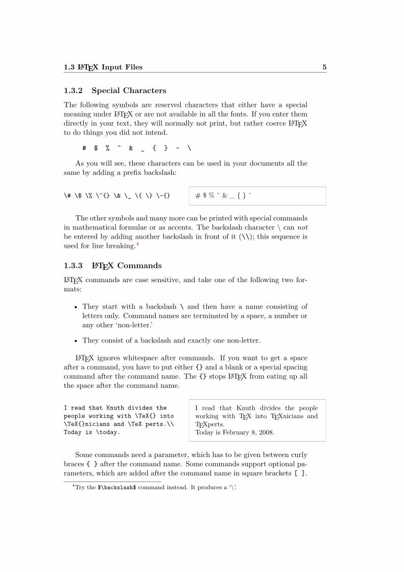
The following symbols are reserved characters that either have a specialmeaning under LATEX or are not available in all the fonts. If you enter themdirectly in your text, they will normally not print, but rather coerce LATEXto do things you did not intend.

# $ % ^ & _ ~ \

As you will see, these characters can be used in your documents all thesame by adding a prefix backslash:

\# \$ \% \^ \& \_ \ \ \~ # $ % ˆ & _ ˜

The other symbols and many more can be printed with special commandsin mathematical formulae or as accents. The backslash character \ can notbe entered by adding another backslash in front of it (\\); this sequence isused for line breaking.4

1.3.3 LATEX Commands

LATEX commands are case sensitive, and take one of the following two for-mats:

• They start with a backslash \ and then have a name consisting ofletters only. Command names are terminated by a space, a number orany other ‘non-letter.’

• They consist of a backslash and exactly one non-letter.

LATEX ignores whitespace after commands. If you want to get a spaceafter a command, you have to put either and a blank or a special spacingcommand after the command name. The stops LATEX from eating up allthe space after the command name.

I read that Knuth divides thepeople working with \TeX into\TeXnicians and \TeX perts.\\Today is \today.

I read that Knuth divides the peopleworking with TEX into TEXnicians andTEXperts.Today is February 8, 2008.

Some commands need a parameter, which has to be given between curlybraces after the command name. Some commands support optional pa-rameters, which are added after the command name in square brackets [ ].

4Try the $\backslash$ command instead. It produces a ‘\’.

6 Things You Need to Know

The next examples use some LATEX commands. Don’t worry about them;they will be explained later.

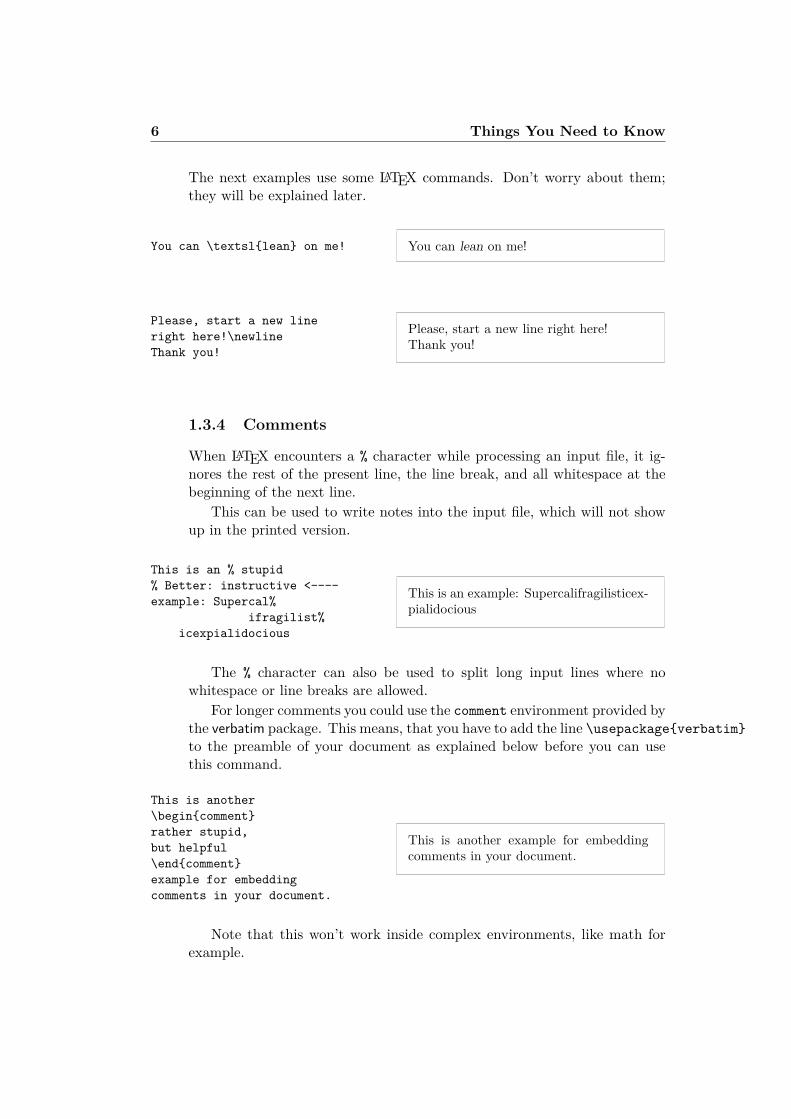
You can \textsllean on me! You can lean on me!

Please, start a new lineright here!\newlineThank you!

Please, start a new line right here!Thank you!

1.3.4 Comments

When LATEX encounters a % character while processing an input file, it ig-nores the rest of the present line, the line break, and all whitespace at thebeginning of the next line.

This can be used to write notes into the input file, which will not showup in the printed version.

This is an % stupid% Better: instructive <----example: Supercal%

ifragilist%icexpialidocious

This is an example: Supercalifragilisticex-pialidocious

The % character can also be used to split long input lines where nowhitespace or line breaks are allowed.

For longer comments you could use the comment environment provided bythe verbatim package. This means, that you have to add the line \usepackageverbatimto the preamble of your document as explained below before you can usethis command.

This is another\begincommentrather stupid,but helpful\endcommentexample for embeddingcomments in your document.

This is another example for embeddingcomments in your document.

Note that this won’t work inside complex environments, like math forexample.

1.4 Input File Structure 7

1.4 Input File StructureWhen LATEX2ε processes an input file, it expects it to follow a certain struc-ture. Thus every input file must start with the command

\documentclass...

This specifies what sort of document you intend to write. After that, youcan include commands that influence the style of the whole document, oryou can load packages that add new features to the LATEX system. To loadsuch a package you use the command

\usepackage...

When all the setup work is done,5 you start the body of the text withthe command

\begindocument

Now you enter the text mixed with some useful LATEX commands. Atthe end of the document you add the

\enddocument

command, which tells LATEX to call it a day. Anything that follows thiscommand will be ignored by LATEX.

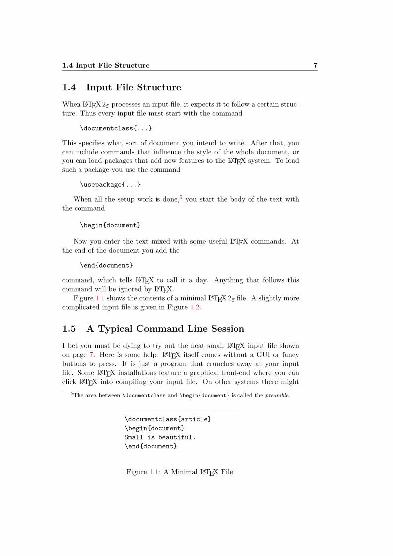
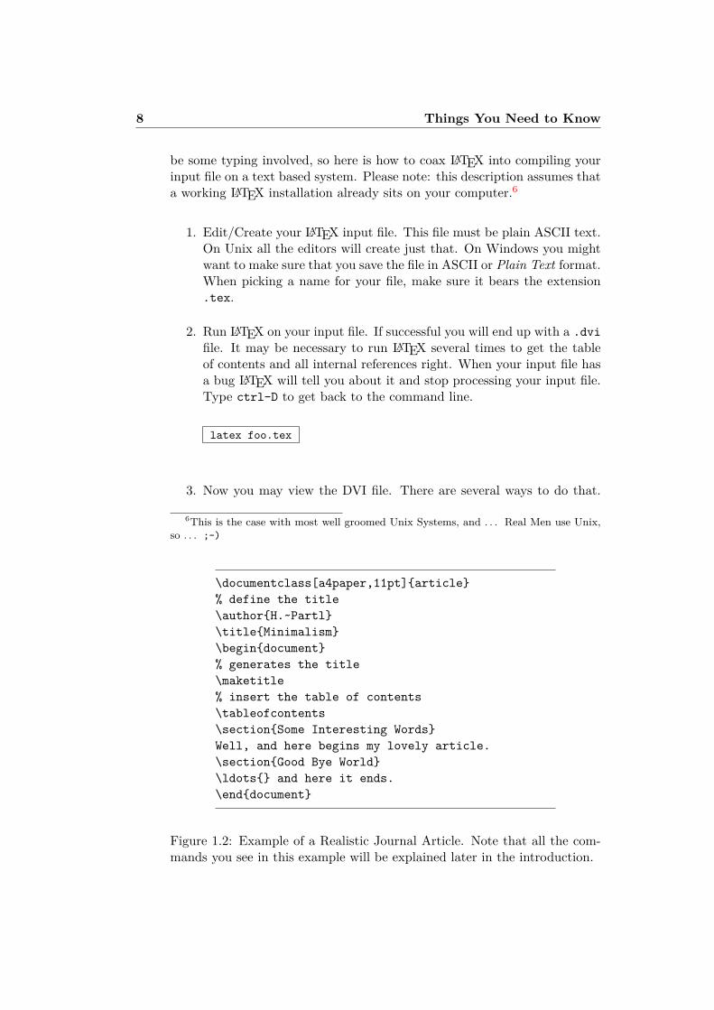
Figure 1.1 shows the contents of a minimal LATEX2ε file. A slightly morecomplicated input file is given in Figure 1.2.

1.5 A Typical Command Line SessionI bet you must be dying to try out the neat small LATEX input file shownon page 7. Here is some help: LATEX itself comes without a GUI or fancybuttons to press. It is just a program that crunches away at your inputfile. Some LATEX installations feature a graphical front-end where you canclick LATEX into compiling your input file. On other systems there might

5The area between \documentclass and \begindocument is called the preamble.

\documentclassarticle\begindocumentSmall is beautiful.\enddocument

Figure 1.1: A Minimal LATEX File.

8 Things You Need to Know

be some typing involved, so here is how to coax LATEX into compiling yourinput file on a text based system. Please note: this description assumes thata working LATEX installation already sits on your computer.6

1. Edit/Create your LATEX input file. This file must be plain ASCII text.On Unix all the editors will create just that. On Windows you mightwant to make sure that you save the file in ASCII or Plain Text format.When picking a name for your file, make sure it bears the extension.tex.

2. Run LATEX on your input file. If successful you will end up with a .dvifile. It may be necessary to run LATEX several times to get the tableof contents and all internal references right. When your input file hasa bug LATEX will tell you about it and stop processing your input file.Type ctrl-D to get back to the command line.

latex foo.tex

3. Now you may view the DVI file. There are several ways to do that.

6This is the case with most well groomed Unix Systems, and . . . Real Men use Unix,so . . . ;-)

\documentclass[a4paper,11pt]article% define the title\authorH.~Partl\titleMinimalism\begindocument% generates the title\maketitle% insert the table of contents\tableofcontents\sectionSome Interesting WordsWell, and here begins my lovely article.\sectionGood Bye World\ldots and here it ends.\enddocument

Figure 1.2: Example of a Realistic Journal Article. Note that all the com-mands you see in this example will be explained later in the introduction.

1.6 The Layout of the Document 9

You can show the file on screen with

xdvi foo.dvi &

This only works on Unix with X11. If you are on Windows you mightwant to try yap (yet another previewer).

You can also convert the dvi file to PostScript for printing or viewingwith Ghostscript.

dvips -Pcmz foo.dvi -o foo.ps

If you are lucky your LATEX system even comes with the dvipdf tool,which allows you to convert your .dvi files straight into pdf.

dvipdf foo.dvi

1.6 The Layout of the Document

1.6.1 Document Classes

The first information LATEX needs to know when processing an input file isthe type of document the author wants to create. This is specified with the\documentclass command.

\documentclass[options]class

Here class specifies the type of document to be created. Table 1.1 lists thedocument classes explained in this introduction. The LATEX2ε distributionprovides additional classes for other documents, including letters and slides.The options parameter customises the behaviour of the document class. Theoptions have to be separated by commas. The most common options for thestandard document classes are listed in Table 1.2.

Example: An input file for a LATEX document could start with the line

\documentclass[11pt,twoside,a4paper]article

which instructs LATEX to typeset the document as an article with a basefont size of eleven points, and to produce a layout suitable for double sidedprinting on A4 paper.

10 Things You Need to Know

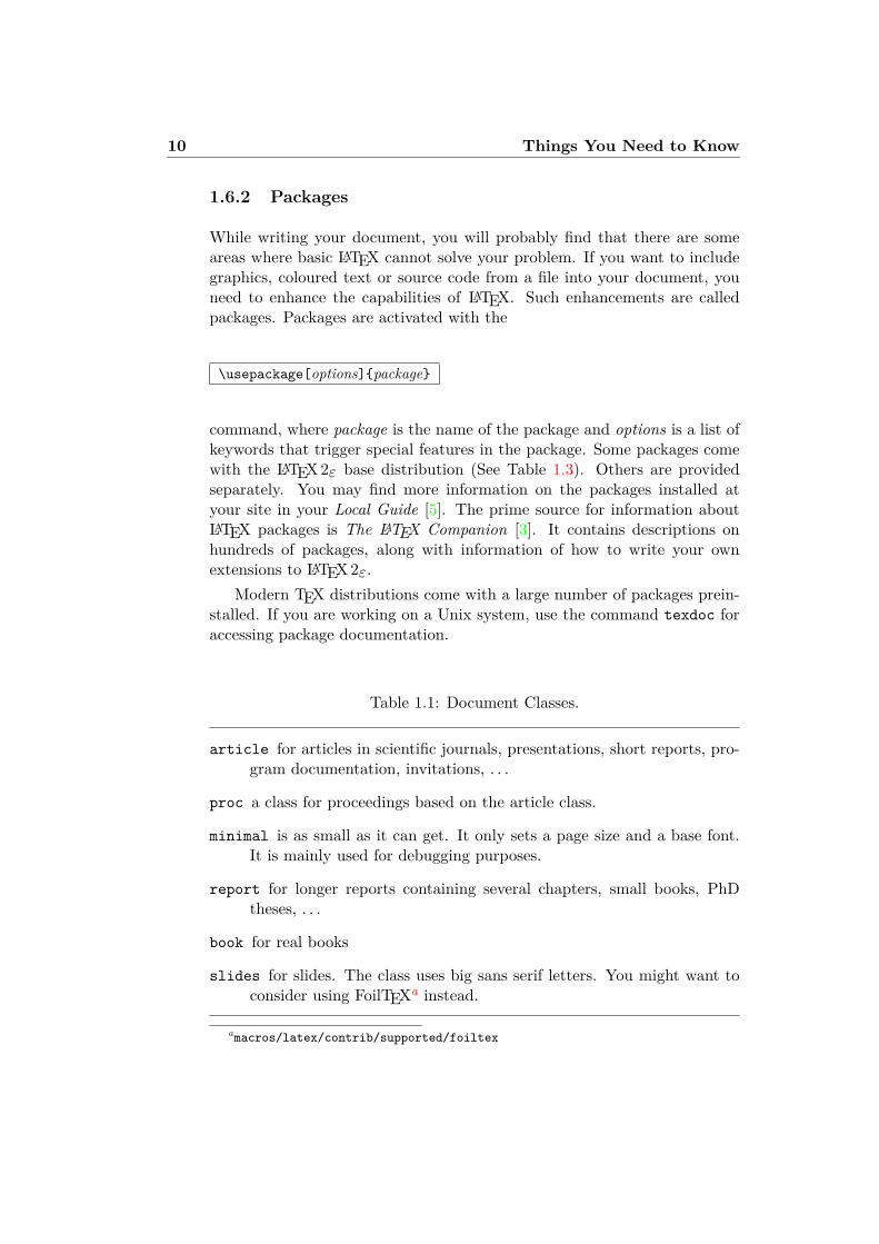
1.6.2 Packages

While writing your document, you will probably find that there are someareas where basic LATEX cannot solve your problem. If you want to includegraphics, coloured text or source code from a file into your document, youneed to enhance the capabilities of LATEX. Such enhancements are calledpackages. Packages are activated with the

\usepackage[options]package

command, where package is the name of the package and options is a list ofkeywords that trigger special features in the package. Some packages comewith the LATEX2ε base distribution (See Table 1.3). Others are providedseparately. You may find more information on the packages installed atyour site in your Local Guide [5]. The prime source for information aboutLATEX packages is The LATEX Companion [3]. It contains descriptions onhundreds of packages, along with information of how to write your ownextensions to LATEX2ε.

Modern TEX distributions come with a large number of packages prein-stalled. If you are working on a Unix system, use the command texdoc foraccessing package documentation.

Table 1.1: Document Classes.

article for articles in scientific journals, presentations, short reports, pro-gram documentation, invitations, . . .

proc a class for proceedings based on the article class.

minimal is as small as it can get. It only sets a page size and a base font.It is mainly used for debugging purposes.

report for longer reports containing several chapters, small books, PhDtheses, . . .

book for real books

slides for slides. The class uses big sans serif letters. You might want toconsider using FoilTEXa instead.

amacros/latex/contrib/supported/foiltex

1.6 The Layout of the Document 11

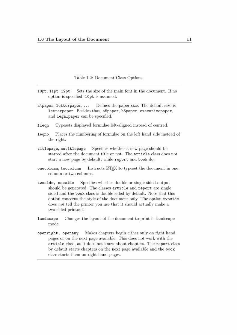
Table 1.2: Document Class Options.

10pt, 11pt, 12pt Sets the size of the main font in the document. If nooption is specified, 10pt is assumed.

a4paper, letterpaper, . . . Defines the paper size. The default size isletterpaper. Besides that, a5paper, b5paper, executivepaper,and legalpaper can be specified.

fleqn Typesets displayed formulae left-aligned instead of centred.

leqno Places the numbering of formulae on the left hand side instead ofthe right.

titlepage, notitlepage Specifies whether a new page should bestarted after the document title or not. The article class does notstart a new page by default, while report and book do.

onecolumn, twocolumn Instructs LATEX to typeset the document in onecolumn or two columns.

twoside, oneside Specifies whether double or single sided outputshould be generated. The classes article and report are singlesided and the book class is double sided by default. Note that thisoption concerns the style of the document only. The option twosidedoes not tell the printer you use that it should actually make atwo-sided printout.

landscape Changes the layout of the document to print in landscapemode.

openright, openany Makes chapters begin either only on right handpages or on the next page available. This does not work with thearticle class, as it does not know about chapters. The report classby default starts chapters on the next page available and the bookclass starts them on right hand pages.

12 Things You Need to Know

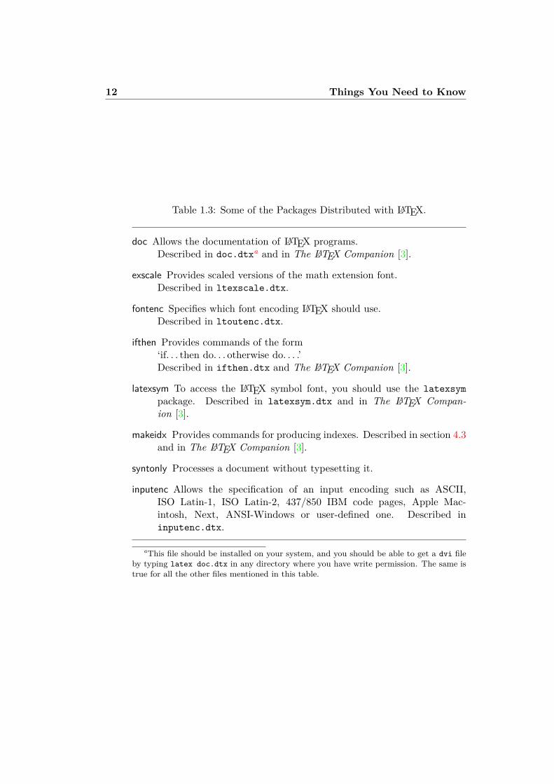
Table 1.3: Some of the Packages Distributed with LATEX.

doc Allows the documentation of LATEX programs.Described in doc.dtxa and in The LATEX Companion [3].

exscale Provides scaled versions of the math extension font.Described in ltexscale.dtx.

fontenc Specifies which font encoding LATEX should use.Described in ltoutenc.dtx.

ifthen Provides commands of the form‘if. . . then do. . . otherwise do. . . .’Described in ifthen.dtx and The LATEX Companion [3].

latexsym To access the LATEX symbol font, you should use the latexsympackage. Described in latexsym.dtx and in The LATEX Compan-ion [3].

makeidx Provides commands for producing indexes. Described in section 4.3and in The LATEX Companion [3].

syntonly Processes a document without typesetting it.

inputenc Allows the specification of an input encoding such as ASCII,ISO Latin-1, ISO Latin-2, 437/850 IBM code pages, Apple Mac-intosh, Next, ANSI-Windows or user-defined one. Described ininputenc.dtx.

aThis file should be installed on your system, and you should be able to get a dvi fileby typing latex doc.dtx in any directory where you have write permission. The same istrue for all the other files mentioned in this table.

1.7 Files You Might Encounter 13

1.6.3 Page Styles

LATEX supports three predefined header/footer combinations—so-called pagestyles. The style parameter of the

\pagestylestyle

command defines which one to use. Table 1.4 lists the predefined page styles.

Table 1.4: The Predefined Page Styles of LATEX.

plain prints the page numbers on the bottom of the page, in the middle ofthe footer. This is the default page style.

headings prints the current chapter heading and the page number in theheader on each page, while the footer remains empty. (This is the styleused in this document)

empty sets both the header and the footer to be empty.

It is possible to change the page style of the current page with the com-mand

\thispagestylestyle

A description how to create your own headers and footers can be foundin The LATEX Companion [3] and in section 4.4 on page 76.

1.7 Files You Might EncounterWhen you work with LATEX you will soon find yourself in a maze of fileswith various extensions and probably no clue. The following list explainsthe various file types you might encounter when working with TEX. Pleasenote that this table does not claim to be a complete list of extensions, butif you find one missing that you think is important, please drop me a line.

.tex LATEX or TEX input file. Can be compiled with latex.

.sty LATEX Macro package. This is a file you can load into your LATEXdocument using the \usepackage command.

.dtx Documented TEX. This is the main distribution format for LATEX stylefiles. If you process a .dtx file you get documented macro code of theLATEX package contained in the .dtx file.

14 Things You Need to Know

.ins The installer for the files contained in the matching .dtx file. If youdownload a LATEX package from the net, you will normally get a .dtxand a .ins file. Run LATEX on the .ins file to unpack the .dtx file.

.cls Class files define what your document looks like. They are selectedwith the \documentclass command.

.fd Font description file telling LATEX about new fonts.

The following files are generated when you run LATEX on your input file:

.dvi Device Independent File. This is the main result of a LATEX compilerun. You can look at its content with a DVI previewer program or youcan send it to a printer with dvips or a similar application.

.log Gives a detailed account of what happened during the last compilerrun.

.toc Stores all your section headers. It gets read in for the next compilerrun and is used to produce the table of content.

.lof This is like .toc but for the list of figures.

.lot And again the same for the list of tables.

.aux Another file that transports information from one compiler run to thenext. Among other things, the .aux file is used to store informationassociated with cross-references.

.idx If your document contains an index. LATEX stores all the words thatgo into the index in this file. Process this file with makeindex. Referto section 4.3 on page 75 for more information on indexing.

.ind The processed .idx file, ready for inclusion into your document on thenext compile cycle.

.ilg Logfile telling what makeindex did.

1.8 Big ProjectsWhen working on big documents, you might want to split the input file intoseveral parts. LATEX has two commands that help you to do that.

\includefilename

You can use this command in the document body to insert the contentsof another file named filename.tex. Note that LATEX will start a new pagebefore processing the material input from filename.tex.

1.8 Big Projects 15

The second command can be used in the preamble. It allows you toinstruct LATEX to only input some of the \included files.

\includeonlyfilename,filename,. . .

After this command is executed in the preamble of the document, only\include commands for the filenames that are listed in the argument ofthe \includeonly command will be executed. Note that there must be nospaces between the filenames and the commas.

The \include command starts typesetting the included text on a newpage. This is helpful when you use \includeonly, because the page breakswill not move, even when some included files are omitted. Sometimes thismight not be desirable. In this case, you can use the

\inputfilename

command. It simply includes the file specified. No flashy suits, no stringsattached.

To make LATEX quickly check your document you can use the syntonlypackage. This makes LATEX skim through your document only checking forproper syntax and usage of the commands, but doesn’t produce any (DVI)output. As LATEX runs faster in this mode you may save yourself valuabletime. Usage is very simple:

\usepackagesyntonly\syntaxonly

When you want to produce pages, just comment out the second line (byadding a percent sign).

Chapter 2

Typesetting Text

After reading the previous chapter, you should know about the basic stuff ofwhich a LATEX2ε document is made. In this chapter I will fill in the remainingstructure you will need to know in order to produce real world material.

2.1 The Structure of Text and LanguageBy Hanspeter Schmid <hanspi@schmid-werren.ch>

The main point of writing a text (some modern DAAC1 literature excluded),is to convey ideas, information, or knowledge to the reader. The reader willunderstand the text better if these ideas are well-structured, and will seeand feel this structure much better if the typographical form reflects thelogical and semantical structure of the content.

LATEX is different from other typesetting systems in that you just haveto tell it the logical and semantical structure of a text. It then derivesthe typographical form of the text according to the “rules” given in thedocument class file and in various style files.

The most important text unit in LATEX (and in typography) is the para-graph. We call it “text unit” because a paragraph is the typographical formthat should reflect one coherent thought, or one idea. You will learn in thefollowing sections how you can force line breaks with e.g. \\, and paragraphbreaks with e.g. leaving an empty line in the source code. Therefore, if anew thought begins, a new paragraph should begin, and if not, only linebreaks should be used. If in doubt about paragraph breaks, think aboutyour text as a conveyor of ideas and thoughts. If you have a paragraphbreak, but the old thought continues, it should be removed. If some totallynew line of thought occurs in the same paragraph, then it should be broken.

Most people completely underestimate the importance of well-placedparagraph breaks. Many people do not even know what the meaning of

1Different At All Cost, a translation of the Swiss German UVA (Um’s Verrecken An-ders).

18 Typesetting Text

a paragraph break is, or, especially in LATEX, introduce paragraph breakswithout knowing it. The latter mistake is especially easy to make if equa-tions are used in the text. Look at the following examples, and figure outwhy sometimes empty lines (paragraph breaks) are used before and after theequation, and sometimes not. (If you don’t yet understand all commandswell enough to understand these examples, please read this and the followingchapter, and then read this section again.)

% Example 1\ldots when Einstein introduced his formula\beginequation

e = m \cdot c^2 \; ,\endequationwhich is at the same time the most widely knownand the least well understood physical formula.

% Example 2\ldots from which follows Kirchhoff’s current law:\beginequation

\sum_k=1^n I_k = 0 \; .\endequation

Kirchhoff’s voltage law can be derived \ldots

% Example 3\ldots which has several advantages.

\beginequationI_D = I_F - I_R

\endequationis the core of a very different transistor model. \ldots

The next smaller text unit is a sentence. In English texts, there is alarger space after a period that ends a sentence than after one that ends anabbreviation. LATEX tries to figure out which one you wanted to have. IfLATEX gets it wrong, you must tell it what you want. This is explained laterin this chapter.

The structuring of text even extends to parts of sentences. Most lan-guages have very complicated punctuation rules, but in many languages(including German and English), you will get almost every comma right ifyou remember what it represents: a short stop in the flow of language. Ifyou are not sure about where to put a comma, read the sentence aloud and

2.2 Line Breaking and Page Breaking 19

take a short breath at every comma. If this feels awkward at some place,delete that comma; if you feel the urge to breathe (or make a short stop) atsome other place, insert a comma.

Finally, the paragraphs of a text should also be structured logically at ahigher level, by putting them into chapters, sections, subsections, and so on.However, the typographical effect of writing e.g. \sectionThe Structureof Text and Language is so obvious that it is almost self-evident howthese high-level structures should be used.

2.2 Line Breaking and Page Breaking

2.2.1 Justified Paragraphs

Books are often typeset with each line having the same length. LATEX insertsthe necessary line breaks and spaces between words by optimizing the con-tents of a whole paragraph. If necessary, it also hyphenates words that wouldnot fit comfortably on a line. How the paragraphs are typeset depends onthe document class. Normally the first line of a paragraph is indented, andthere is no additional space between two paragraphs. Refer to section 6.3.2for more information.

In special cases it might be necessary to order LATEX to break a line:

\\ or \newline

starts a new line without starting a new paragraph.

\\*

additionally prohibits a page break after the forced line break.

\newpage

starts a new page.

\linebreak[n], \nolinebreak[n], \pagebreak[n], \nopagebreak[n]

suggest places where a break may (or may not happen). They enable theauthor to influence their actions with the optional argument n, which canbe set to a number between zero and four. By setting n to a value below4, you leave LATEX the option of ignoring your command if the result wouldlook very bad. Do not confuse these “break” commands with the “new”commands. Even when you give a “break” command, LATEX still tries toeven out the right border of the line and the total length of the page, asdescribed in the next section; this can lead to unpleasant gaps in your text.

20 Typesetting Text

If you really want to start a “new line” or a “new page”, then use thecorresponding command. Guess their names!

LATEX always tries to produce the best line breaks possible. If it cannotfind a way to break the lines in a manner that meets its high standards, itlets one line stick out on the right of the paragraph. LATEX then complains(“overfull hbox”) while processing the input file. This happens most oftenwhen LATEX cannot find a suitable place to hyphenate a word.2 You can in-struct LATEX to lower its standards a little by giving the \sloppy command.It prevents such over-long lines by increasing the inter-word spacing—evenif the final output is not optimal. In this case a warning (“underfull hbox”)is given to the user. In most such cases the result doesn’t look very good.The command \fussy brings LATEX back to its default behaviour.

2.2.2 Hyphenation

LATEX hyphenates words whenever necessary. If the hyphenation algorithmdoes not find the correct hyphenation points, you can remedy the situationby using the following commands to tell TEX about the exception.

The command

\hyphenationword list

causes the words listed in the argument to be hyphenated only at the pointsmarked by “-”. The argument of the command should only contain wordsbuilt from normal letters, or rather signs that are considered to be normalletters by LATEX. The hyphenation hints are stored for the language thatis active when the hyphenation command occurs. This means that if youplace a hyphenation command into the preamble of your document it willinfluence the English language hyphenation. If you place the commandafter the \begindocument and you are using some package for nationallanguage support like babel, then the hyphenation hints will be active in thelanguage activated through babel.

The example below will allow “hyphenation” to be hyphenated as wellas “Hyphenation”, and it prevents “FORTRAN”, “Fortran” and “fortran”from being hyphenated at all. No special characters or symbols are allowedin the argument.

Example:

\hyphenationFORTRAN Hy-phen-a-tion

2Although LATEX gives you a warning when that happens (Overfull hbox) and displaysthe offending line, such lines are not always easy to find. If you use the option draft inthe \documentclass command, these lines will be marked with a thick black line on theright margin.

2.3 Ready-Made Strings 21

The command \- inserts a discretionary hyphen into a word. This alsobecomes the only point hyphenation is allowed in this word. This commandis especially useful for words containing special characters (e.g. accentedcharacters), because LATEX does not automatically hyphenate words con-taining special characters.

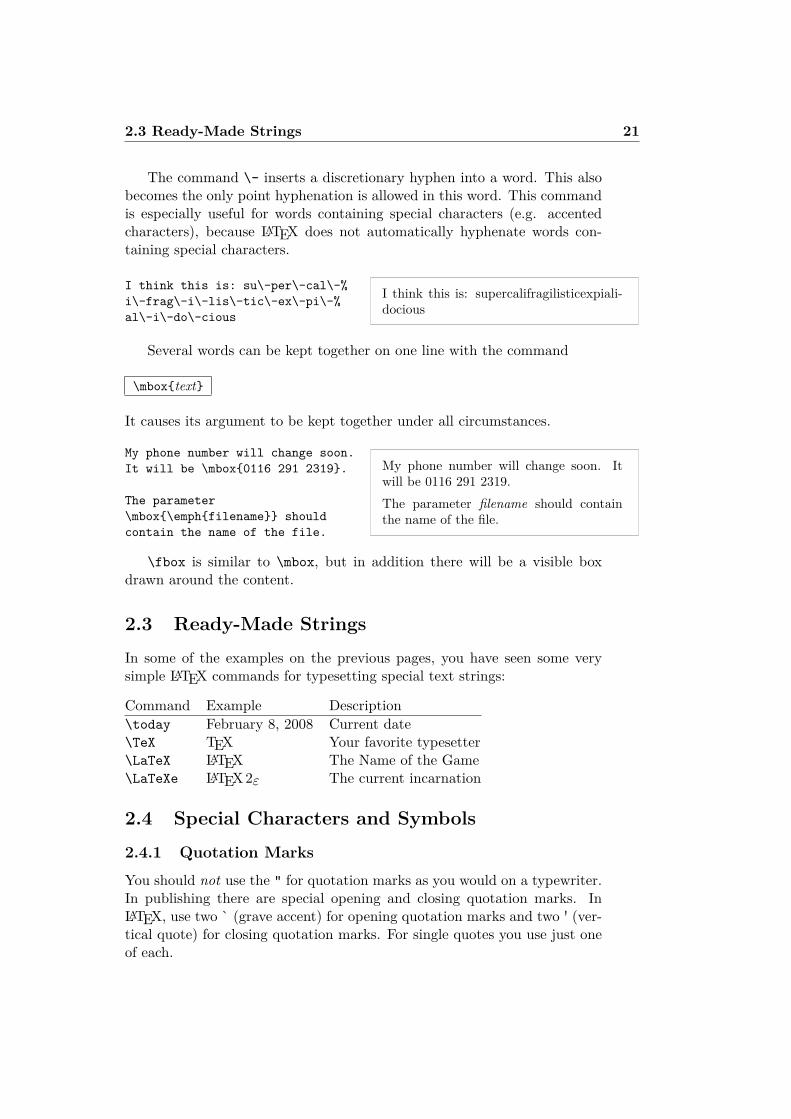
I think this is: su\-per\-cal\-%i\-frag\-i\-lis\-tic\-ex\-pi\-%al\-i\-do\-cious

I think this is: supercalifragilisticexpiali-docious

Several words can be kept together on one line with the command

\mboxtext

It causes its argument to be kept together under all circumstances.

My phone number will change soon.It will be \mbox0116 291 2319.

The parameter\mbox\emphfilename shouldcontain the name of the file.

My phone number will change soon. Itwill be 0116 291 2319.The parameter filename should containthe name of the file.

\fbox is similar to \mbox, but in addition there will be a visible boxdrawn around the content.

2.3 Ready-Made StringsIn some of the examples on the previous pages, you have seen some verysimple LATEX commands for typesetting special text strings:

Command Example Description\today February 8, 2008 Current date\TeX TEX Your favorite typesetter\LaTeX LATEX The Name of the Game\LaTeXe LATEX2ε The current incarnation

2.4 Special Characters and Symbols

2.4.1 Quotation Marks

You should not use the " for quotation marks as you would on a typewriter.In publishing there are special opening and closing quotation marks. InLATEX, use two ` (grave accent) for opening quotation marks and two ' (ver-tical quote) for closing quotation marks. For single quotes you use just oneof each.

22 Typesetting Text

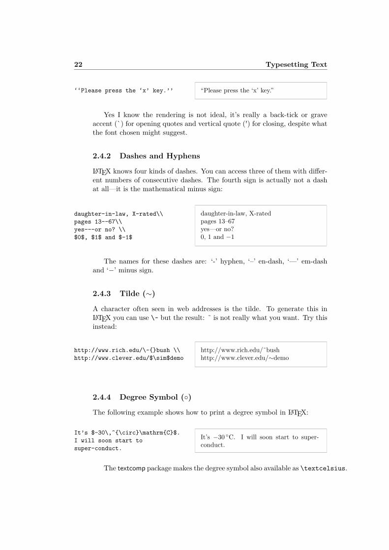
‘‘Please press the ‘x’ key.’’ “Please press the ‘x’ key.”

Yes I know the rendering is not ideal, it’s really a back-tick or graveaccent (`) for opening quotes and vertical quote (') for closing, despite whatthe font chosen might suggest.

2.4.2 Dashes and Hyphens

LATEX knows four kinds of dashes. You can access three of them with differ-ent numbers of consecutive dashes. The fourth sign is actually not a dashat all—it is the mathematical minus sign:

daughter-in-law, X-rated\\pages 13--67\\yes---or no? \\$0$, $1$ and $-1$

daughter-in-law, X-ratedpages 13–67yes—or no?0, 1 and −1

The names for these dashes are: ‘-’ hyphen, ‘–’ en-dash, ‘—’ em-dashand ‘−’ minus sign.

2.4.3 Tilde (∼)

A character often seen in web addresses is the tilde. To generate this inLATEX you can use \~ but the result: ˜ is not really what you want. Try thisinstead:

http://www.rich.edu/\~bush \\http://www.clever.edu/$\sim$demo

http://www.rich.edu/˜bushhttp://www.clever.edu/∼demo

2.4.4 Degree Symbol ()

The following example shows how to print a degree symbol in LATEX:

It’s $-30\,^\circ\mathrmC$.I will soon start tosuper-conduct.

It’s −30 C. I will soon start to super-conduct.

The textcomp package makes the degree symbol also available as \textcelsius.

2.4 Special Characters and Symbols 23

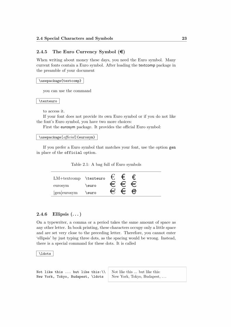
2.4.5 The Euro Currency Symbol (e)

When writing about money these days, you need the Euro symbol. Manycurrent fonts contain a Euro symbol. After loading the textcomp package inthe preamble of your document

\usepackagetextcomp

you can use the command

\texteuro

to access it.If your font does not provide its own Euro symbol or if you do not like

the font’s Euro symbol, you have two more choices:First the eurosym package. It provides the official Euro symbol:

\usepackage[official]eurosym

If you prefer a Euro symbol that matches your font, use the option genin place of the official option.

Table 2.1: A bag full of Euro symbols

LM+textcomp \texteuro € € €eurosym \euro e e e[gen]eurosym \euro AC AC AC

2.4.6 Ellipsis (. . . )

On a typewriter, a comma or a period takes the same amount of space asany other letter. In book printing, these characters occupy only a little spaceand are set very close to the preceding letter. Therefore, you cannot enter‘ellipsis’ by just typing three dots, as the spacing would be wrong. Instead,there is a special command for these dots. It is called

\ldots

Not like this ... but like this:\\New York, Tokyo, Budapest, \ldots

Not like this ... but like this:New York, Tokyo, Budapest, . . .

24 Typesetting Text

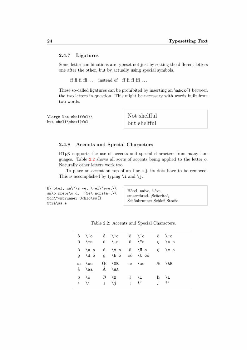
2.4.7 Ligatures

Some letter combinations are typeset not just by setting the different lettersone after the other, but by actually using special symbols.

ff fi fl ffi. . . instead of ff fi fl ffi . . .

These so-called ligatures can be prohibited by inserting an \mbox betweenthe two letters in question. This might be necessary with words built fromtwo words.

\Large Not shelfful\\but shelf\mboxful

Not shelffulbut shelfful

2.4.8 Accents and Special Characters

LATEX supports the use of accents and special characters from many lan-guages. Table 2.2 shows all sorts of accents being applied to the letter o.Naturally other letters work too.

To place an accent on top of an i or a j, its dots have to be removed.This is accomplished by typing \i and \j.

H\^otel, na\"\i ve, \’el\‘eve,\\sm\o rrebr\o d, !‘Se\~norita!,\\Sch\"onbrunner Schlo\ssStra\ss e

Hôtel, naïve, élève,smørrebrød, ¡Señorita!,Schönbrunner Schloß Straße

Table 2.2: Accents and Special Characters.

ò \‘o ó \’o ô \^o õ \~oo \=o o \.o ö \"o ç \c c

o \u o o \v o ő \H o o \c oo. \d o o

¯\b o oo \t oo

œ \oe Œ \OE æ \ae Æ \AEå \aa Å \AA

ø \o Ø \O ł \l Ł \Lı \i \j ¡ !‘ ¿ ?‘

2.5 International Language Support 25

2.5 International Language SupportWhen you write documents in languages other than English, there are threeareas where LATEX has to be configured appropriately:

1. All automatically generated text strings3 have to be adapted to thenew language. For many languages, these changes can be accomplishedby using the babel package by Johannes Braams.

2. LATEX needs to know the hyphenation rules for the new language.Getting hyphenation rules into LATEX is a bit more tricky. It meansrebuilding the format file with different hyphenation patterns enabled.Your Local Guide [5] should give more information on this.

3. Language specific typographic rules. In French for example, there is amandatory space before each colon character (:).

If your system is already configured appropriately, you can activate thebabel package by adding the command

\usepackage[language]babel

after the \documentclass command. A list of the languages built into yourLATEX system will be displayed every time the compiler is started. Babel willautomatically activate the appropriate hyphenation rules for the languageyou choose. If your LATEX format does not support hyphenation in thelanguage of your choice, babel will still work but will disable hyphenation,which has quite a negative effect on the appearance of the typeset document.

Babel also specifies new commands for some languages, which simplifythe input of special characters. The German language, for example, containsa lot of umlauts (äöü). With babel, you can enter an ö by typing "o insteadof \"o.

If you call babel with multiple languages

\usepackage[languageA,languageB]babel

then the last language in the option list will be active (i.e. languageB). Youcan to use the command

\selectlanguagelanguageA

to change the active language.Most of the modern computer systems allow you to input letter of na-

tional alphabets directly from the keyboard. In order to handle variety of3Table of Contents, List of Figures, . . .

26 Typesetting Text

input encoding used for different groups of languages and/or on differentcomputer platforms LATEX employs the inputenc package:

\usepackage[encoding]inputenc

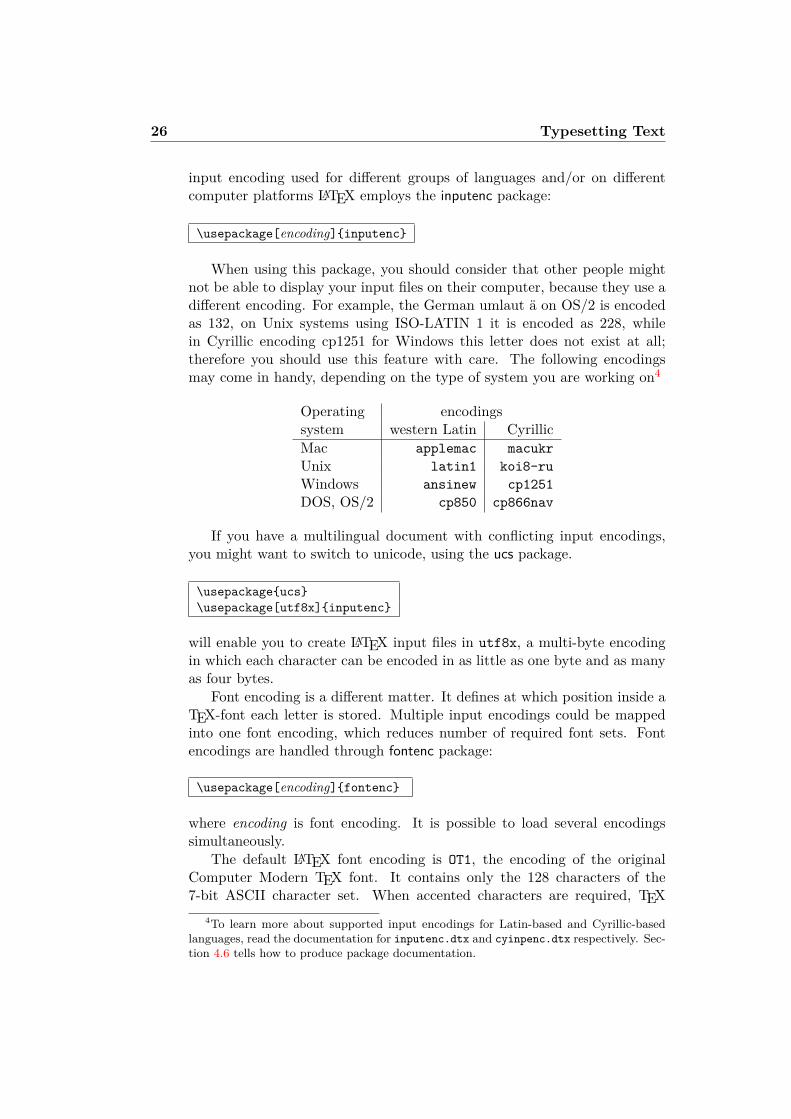
When using this package, you should consider that other people mightnot be able to display your input files on their computer, because they use adifferent encoding. For example, the German umlaut ä on OS/2 is encodedas 132, on Unix systems using ISO-LATIN 1 it is encoded as 228, whilein Cyrillic encoding cp1251 for Windows this letter does not exist at all;therefore you should use this feature with care. The following encodingsmay come in handy, depending on the type of system you are working on4

Operating encodingssystem western Latin CyrillicMac applemac macukrUnix latin1 koi8-ruWindows ansinew cp1251DOS, OS/2 cp850 cp866nav

If you have a multilingual document with conflicting input encodings,you might want to switch to unicode, using the ucs package.

\usepackageucs\usepackage[utf8x]inputenc

will enable you to create LATEX input files in utf8x, a multi-byte encodingin which each character can be encoded in as little as one byte and as manyas four bytes.

Font encoding is a different matter. It defines at which position inside aTEX-font each letter is stored. Multiple input encodings could be mappedinto one font encoding, which reduces number of required font sets. Fontencodings are handled through fontenc package:

\usepackage[encoding]fontenc

where encoding is font encoding. It is possible to load several encodingssimultaneously.

The default LATEX font encoding is OT1, the encoding of the originalComputer Modern TEX font. It contains only the 128 characters of the7-bit ASCII character set. When accented characters are required, TEX

4To learn more about supported input encodings for Latin-based and Cyrillic-basedlanguages, read the documentation for inputenc.dtx and cyinpenc.dtx respectively. Sec-tion 4.6 tells how to produce package documentation.

2.5 International Language Support 27

creates them by combining a normal character with an accent. While theresulting output looks perfect, this approach stops the automatic hyphen-ation from working inside words containing accented characters. Besides,some of Latin letters could not be created by combining a normal characterwith an accent, to say nothing about letters of non-Latin alphabets, such asGreek or Cyrillic.

To overcome these shortcomings, several 8-bit CM-like font sets werecreated. Extended Cork (EC) fonts in T1 encoding contains letters andpunctuation characters for most of the European languages based on Latinscript. The LH font set contains letters necessary to typeset documentsin languages using Cyrillic script. Because of the large number of Cyrillicglyphs, they are arranged into four font encodings—T2A, T2B, T2C, and X2.5The CB bundle contains fonts in LGR encoding for the composition of Greektext.

By using these fonts you can improve/enable hyphenation in non-Englishdocuments. Another advantage of using new CM-like fonts is that theyprovide fonts of CM families in all weights, shapes, and optically scaled fontsizes.

2.5.1 Support for PortugueseBy Demerson Andre Polli <polli@linux.ime.usp.br>

To enable hyphenation and change all automatic text to Portuguese, use thecommand:

\usepackage[portuguese]babel

Or if you are in Brazil, substitute the language for brazilian.As there are a lot of accents in Portuguese you might want to use

\usepackage[latin1]inputenc

to be able to input them correctly as well as

\usepackage[T1]fontenc

to get the hyphenation right.See table 2.3 for the preamble you need to write in the Portuguese lan-

guage. Note that we are using the latin1 input encoding here, so this willnot work on a Mac or on DOS. Just use the appropriate encoding for yoursystem.

5The list of languages supported by each of these encodings could be found in [11].

28 Typesetting Text

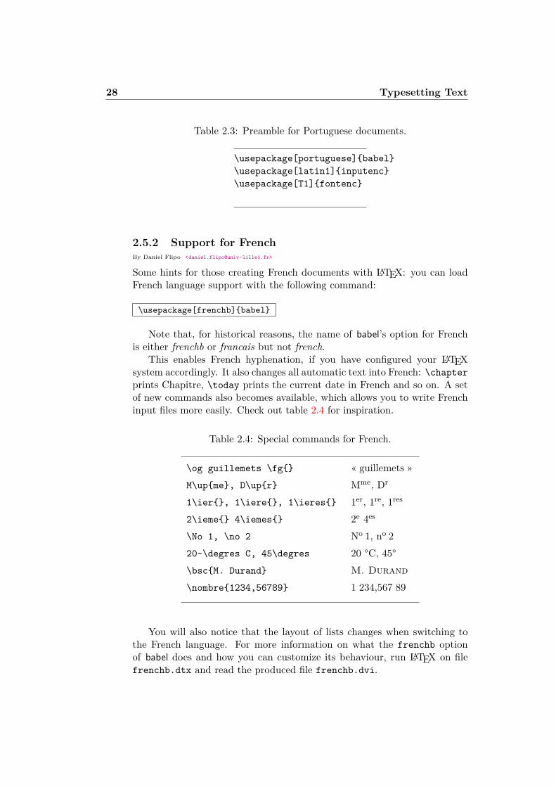
Table 2.3: Preamble for Portuguese documents.

\usepackage[portuguese]babel\usepackage[latin1]inputenc\usepackage[T1]fontenc

2.5.2 Support for FrenchBy Daniel Flipo <daniel.flipo@univ-lille1.fr>

Some hints for those creating French documents with LATEX: you can loadFrench language support with the following command:

\usepackage[frenchb]babel

Note that, for historical reasons, the name of babel’s option for Frenchis either frenchb or francais but not french.

This enables French hyphenation, if you have configured your LATEXsystem accordingly. It also changes all automatic text into French: \chapterprints Chapitre, \today prints the current date in French and so on. A setof new commands also becomes available, which allows you to write Frenchinput files more easily. Check out table 2.4 for inspiration.

Table 2.4: Special commands for French.

\og guillemets \fg « guillemets »M\upme, D\upr Mme, Dr

1\ier, 1\iere, 1\ieres 1er, 1re, 1res

2\ieme 4\iemes 2e 4es

\No 1, \no 2 No 1, no 220~\degres C, 45\degres 20 °C, 45°\bscM. Durand M. Durand\nombre1234,56789 1 234,567 89

You will also notice that the layout of lists changes when switching tothe French language. For more information on what the frenchb optionof babel does and how you can customize its behaviour, run LATEX on filefrenchb.dtx and read the produced file frenchb.dvi.

2.5 International Language Support 29

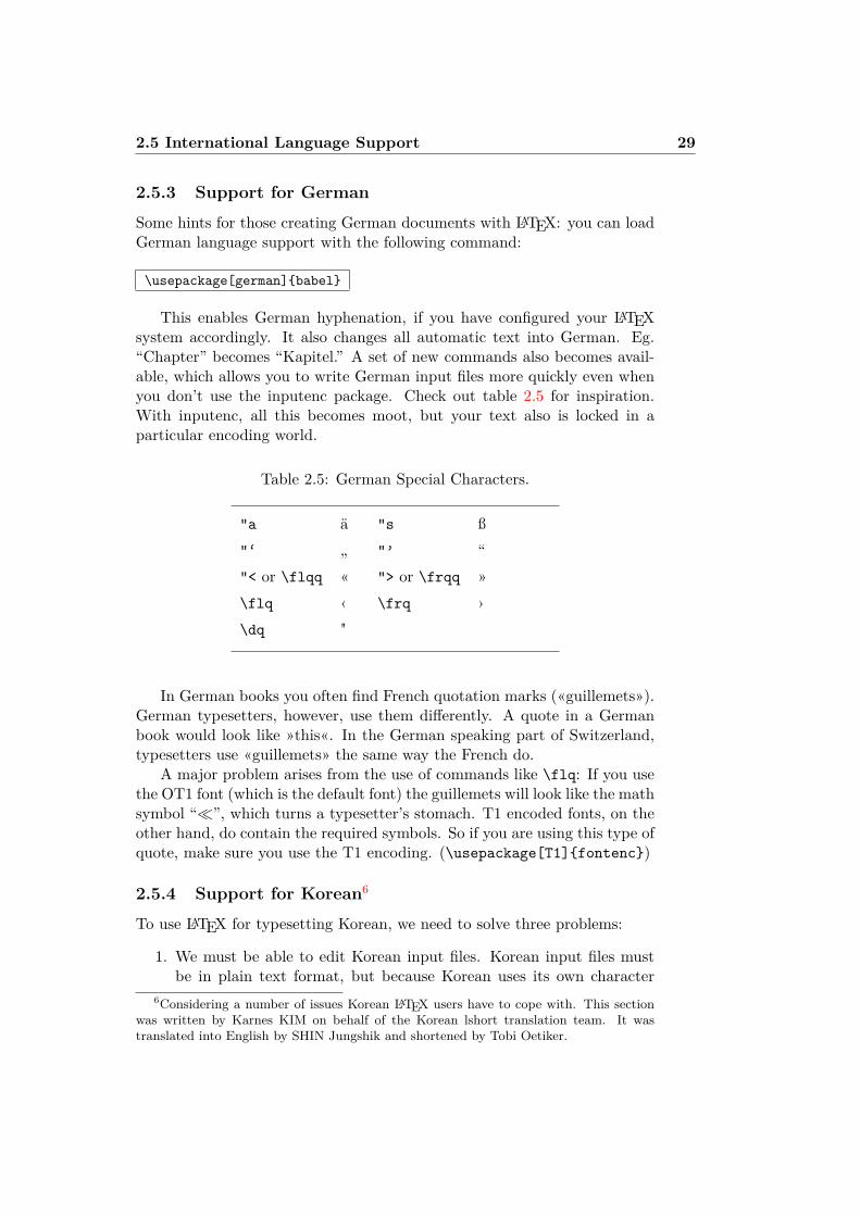
2.5.3 Support for German

Some hints for those creating German documents with LATEX: you can loadGerman language support with the following command:

\usepackage[german]babel

This enables German hyphenation, if you have configured your LATEXsystem accordingly. It also changes all automatic text into German. Eg.“Chapter” becomes “Kapitel.” A set of new commands also becomes avail-able, which allows you to write German input files more quickly even whenyou don’t use the inputenc package. Check out table 2.5 for inspiration.With inputenc, all this becomes moot, but your text also is locked in aparticular encoding world.

Table 2.5: German Special Characters.

"a ä "s ß"‘ „ "’ “"< or \flqq « "> or \frqq »\flq ‹ \frq ›\dq "

In German books you often find French quotation marks («guillemets»).German typesetters, however, use them differently. A quote in a Germanbook would look like »this«. In the German speaking part of Switzerland,typesetters use «guillemets» the same way the French do.

A major problem arises from the use of commands like \flq: If you usethe OT1 font (which is the default font) the guillemets will look like the mathsymbol “”, which turns a typesetter’s stomach. T1 encoded fonts, on theother hand, do contain the required symbols. So if you are using this type ofquote, make sure you use the T1 encoding. (\usepackage[T1]fontenc)

2.5.4 Support for Korean6

To use LATEX for typesetting Korean, we need to solve three problems:

1. We must be able to edit Korean input files. Korean input files mustbe in plain text format, but because Korean uses its own character

6Considering a number of issues Korean LATEX users have to cope with. This sectionwas written by Karnes KIM on behalf of the Korean lshort translation team. It wastranslated into English by SHIN Jungshik and shortened by Tobi Oetiker.

30 Typesetting Text

set outside the repertoire of US-ASCII, they will look rather strangewith a normal ASCII editor. The two most widely used encodings forKorean text files are EUC-KR and its upward compatible extensionused in Korean MS-Windows, CP949/Windows-949/UHC. In theseencodings each US-ASCII character represents its normal ASCII char-acter similar to other ASCII compatible encodings such as ISO-8859-x, EUC-JP, Big5, or Shift_JIS. On the other hand, Hangul syllables,Hanjas (Chinese characters as used in Korea), Hangul Jamos, Hira-ganas, Katakanas, Greek and Cyrillic characters and other symbolsand letters drawn from KS X 1001 are represented by two consecutiveoctets. The first has its MSB set. Until the mid-1990’s, it took aconsiderable amount of time and effort to set up a Korean-capable en-vironment under a non-localized (non-Korean) operating system. Youcan skim through the now much-outdated http://jshin.net/faq toget a glimpse of what it was like to use Korean under non-Korean OSin mid-1990’s. These days all three major operating systems (Mac OS,Unix, Windows) come equipped with pretty decent multilingual sup-port and internationalization features so that editing Korean text fileis not so much of a problem anymore, even on non-Korean operatingsystems.

2. TEX and LATEX were originally written for scripts with no more than256 characters in their alphabet. To make them work for languageswith considerably more characters such as Korean7 or Chinese, a sub-font mechanism was developed. It divides a single CJK font withthousands or tens of thousands of glyphs into a set of subfonts with256 glyphs each. For Korean, there are three widely used packages;HLATEX by UN Koaunghi, hLATEXp by CHA Jaechoon and the CJK

7Korean Hangul is an alphabetic script with 14 basic consonants and 10 basic vowels(Jamos). Unlike Latin or Cyrillic scripts, the individual characters have to be arrangedin rectangular clusters about the same size as Chinese characters. Each cluster representsa syllable. An unlimited number of syllables can be formed out of this finite set of vow-els and consonants. Modern Korean orthographic standards (both in South Korea andNorth Korea), however, put some restriction on the formation of these clusters. Thereforeonly a finite number of orthographically correct syllables exist. The Korean Charac-ter encoding defines individual code points for each of these syllables (KS X 1001:1998and KS X 1002:1992). So Hangul, albeit alphabetic, is treated like the Chinese andJapanese writing systems with tens of thousands of ideographic/logographic characters.ISO 10646/Unicode offers both ways of representing Hangul used for modern Korean byencoding Conjoining Hangul Jamos (alphabets: http://www.unicode.org/charts/PDF/U1100.pdf) in addition to encoding all the orthographically allowed Hangul syllables inmodern Korean (http://www.unicode.org/charts/PDF/UAC00.pdf). One of the mostdaunting challenges in Korean typesetting with LATEX and related typesetting system issupporting Middle Korean—and possibly future Korean—syllables that can be only rep-resented by conjoining Jamos in Unicode. It is hoped that future TEX engines like Ω andΛ will eventually provide solutions to this so that some Korean linguists and historianswill defect from MS Word that already has a pretty good support for Middle Korean.

2.5 International Language Support 31

package by Werner Lemberg.8 HLATEX and hLATEXp are specific to Ko-rean and provide Korean localization on top of the font support. Theyboth can process Korean input text files encoded in EUC-KR. HLATEXcan even process input files encoded in CP949/Windows-949/UHC andUTF-8 when used along with Λ, Ω.The CJK package is not specific to Korean. It can process input filesin UTF-8 as well as in various CJK encodings including EUC-KR andCP949/Windows-949/UHC, it can be used to typeset documents withmultilingual content (especially Chinese, Japanese and Korean). TheCJK package has no Korean localization such as the one offered byHLATEX and it does not come with as many special Korean fonts asHLATEX.

3. The ultimate purpose of using typesetting programs like TEX andLATEX is to get documents typeset in an ‘aesthetically’ satisfying way.Arguably the most important element in typesetting is a set of well-designed fonts. The HLATEX distribution includes UHC PostScriptfonts of 10 different families and Munhwabu9 fonts (TrueType) of 5different families. The CJK package works with a set of fonts used byearlier versions of HLATEX and it can use Bitstream’s cyberbit True-Type font.

To use the HLATEX package for typesetting your Korean text, put thefollowing declaration into the preamble of your document:

\usepackagehangul

This command turns the Korean localization on. The headings of chap-ters, sections, subsections, table of content and table of figures are all trans-lated into Korean and the formatting of the document is changed to followKorean conventions. The package also provides automatic “particle selec-tion.” In Korean, there are pairs of post-fix particles grammatically equiv-alent but different in form. Which of any given pair is correct depends onwhether the preceding syllable ends with a vowel or a consonant. (It is a bitmore complex than this, but this should give you a good picture.) NativeKorean speakers have no problem picking the right particle, but it cannotbe determined which particle to use for references and other automatic textthat will change while you edit the document. It takes a painstaking effortto place appropriate particles manually every time you add/remove refer-ences or simply shuffle parts of your document around. HLATEX relieves itsusers from this boring and error-prone process.

8They can be obtained at language/korean/HLaTeX/language/korean/CJK/ and http://knot.kaist.ac.kr/htex/

9Korean Ministry of Culture.

32 Typesetting Text

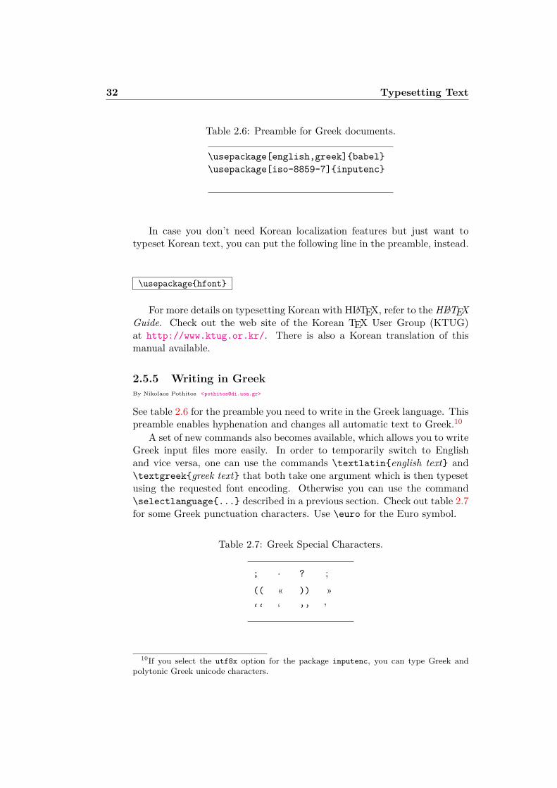
Table 2.6: Preamble for Greek documents.

\usepackage[english,greek]babel\usepackage[iso-8859-7]inputenc

In case you don’t need Korean localization features but just want totypeset Korean text, you can put the following line in the preamble, instead.

\usepackagehfont

For more details on typesetting Korean with HLATEX, refer to the HLATEXGuide. Check out the web site of the Korean TEX User Group (KTUG)at http://www.ktug.or.kr/. There is also a Korean translation of thismanual available.

2.5.5 Writing in GreekBy Nikolaos Pothitos <pothitos@di.uoa.gr>

See table 2.6 for the preamble you need to write in the Greek language. Thispreamble enables hyphenation and changes all automatic text to Greek.10

A set of new commands also becomes available, which allows you to writeGreek input files more easily. In order to temporarily switch to Englishand vice versa, one can use the commands \textlatinenglish text and\textgreekgreek text that both take one argument which is then typesetusing the requested font encoding. Otherwise you can use the command\selectlanguage... described in a previous section. Check out table 2.7for some Greek punctuation characters. Use \euro for the Euro symbol.

Table 2.7: Greek Special Characters.

; · ? ;(( « )) »‘‘ ‘ ’’ ’

10If you select the utf8x option for the package inputenc, you can type Greek andpolytonic Greek unicode characters.

2.6 The Space Between Words 33

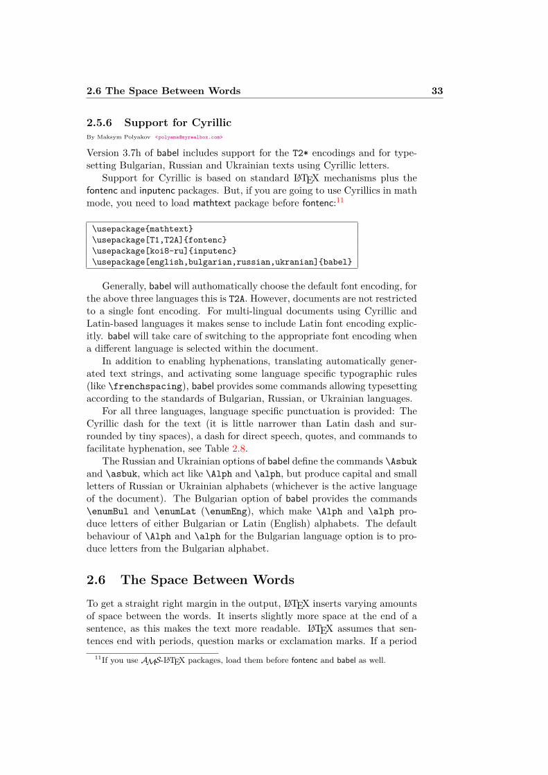
2.5.6 Support for CyrillicBy Maksym Polyakov <polyama@myrealbox.com>

Version 3.7h of babel includes support for the T2* encodings and for type-setting Bulgarian, Russian and Ukrainian texts using Cyrillic letters.

Support for Cyrillic is based on standard LATEX mechanisms plus thefontenc and inputenc packages. But, if you are going to use Cyrillics in mathmode, you need to load mathtext package before fontenc:11

\usepackagemathtext\usepackage[T1,T2A]fontenc\usepackage[koi8-ru]inputenc\usepackage[english,bulgarian,russian,ukranian]babel

Generally, babel will authomatically choose the default font encoding, forthe above three languages this is T2A. However, documents are not restrictedto a single font encoding. For multi-lingual documents using Cyrillic andLatin-based languages it makes sense to include Latin font encoding explic-itly. babel will take care of switching to the appropriate font encoding whena different language is selected within the document.

In addition to enabling hyphenations, translating automatically gener-ated text strings, and activating some language specific typographic rules(like \frenchspacing), babel provides some commands allowing typesettingaccording to the standards of Bulgarian, Russian, or Ukrainian languages.

For all three languages, language specific punctuation is provided: TheCyrillic dash for the text (it is little narrower than Latin dash and sur-rounded by tiny spaces), a dash for direct speech, quotes, and commands tofacilitate hyphenation, see Table 2.8.

The Russian and Ukrainian options of babel define the commands \Asbukand \asbuk, which act like \Alph and \alph, but produce capital and smallletters of Russian or Ukrainian alphabets (whichever is the active languageof the document). The Bulgarian option of babel provides the commands\enumBul and \enumLat (\enumEng), which make \Alph and \alph pro-duce letters of either Bulgarian or Latin (English) alphabets. The defaultbehaviour of \Alph and \alph for the Bulgarian language option is to pro-duce letters from the Bulgarian alphabet.

2.6 The Space Between Words

To get a straight right margin in the output, LATEX inserts varying amountsof space between the words. It inserts slightly more space at the end of asentence, as this makes the text more readable. LATEX assumes that sen-tences end with periods, question marks or exclamation marks. If a period

11If you use AMS-LATEX packages, load them before fontenc and babel as well.

34 Typesetting Text

Table 2.8: The extra definitions made by Bulgarian, Russian, and Ukrainianoptions of babel"| disable ligature at this position."- an explicit hyphen sign, allowing hyphenation in the rest of the word."--- Cyrillic emdash in plain text."--~ Cyrillic emdash in compound names (surnames)."--* Cyrillic emdash for denoting direct speech."" like "-, but producing no hyphen sign (for compound words with

hyphen, e.g.x-""y or some other signs as “disable/enable”)."~ for a compound word mark without a breakpoint."= for a compound word mark with a breakpoint, allowing hyphenation

in the composing words.", thinspace for initials with a breakpoint in following surname."‘ for German left double quotes (looks like ,,)."’ for German right double quotes (looks like “)."< for French left double quotes (looks like <<)."> for French right double quotes (looks like >>).

follows an uppercase letter, this is not taken as a sentence ending, sinceperiods after uppercase letters normally occur in abbreviations.

Any exception from these assumptions has to be specified by the author.A backslash in front of a space generates a space that will not be enlarged. Atilde ‘~’ character generates a space that cannot be enlarged and additionallyprohibits a line break. The command \@ in front of a period specifies thatthis period terminates a sentence even when it follows an uppercase letter.

Mr.~Smith was happy to see her\\cf.~Fig.~5\\I like BASIC\@. What about you?

Mr. Smith was happy to see hercf. Fig. 5I like BASIC. What about you?

The additional space after periods can be disabled with the command

\frenchspacing

which tells LATEX not to insert more space after a period than after ordinarycharacter. This is very common in non-English languages, except bibliogra-phies. If you use \frenchspacing, the command \@ is not necessary.

2.7 Titles, Chapters, and Sections 35

2.7 Titles, Chapters, and Sections

To help the reader find his or her way through your work, you should divideit into chapters, sections, and subsections. LATEX supports this with specialcommands that take the section title as their argument. It is up to you touse them in the correct order.

The following sectioning commands are available for the article class:

\section...\subsection...\subsubsection...\paragraph...\subparagraph...

If you want to split your document in parts without influencing thesection or chapter numbering you can use

\part...

When you work with the report or book class, an additional top-levelsectioning command becomes available

\chapter...

As the article class does not know about chapters, it is quite easyto add articles as chapters to a book. The spacing between sections, thenumbering and the font size of the titles will be set automatically by LATEX.

Two of the sectioning commands are a bit special:

• The \part command does not influence the numbering sequence ofchapters.

• The \appendix command does not take an argument. It just changesthe chapter numbering to letters.12

LATEX creates a table of contents by taking the section headings and pagenumbers from the last compile cycle of the document. The command

\tableofcontents

expands to a table of contents at the place it is issued. A new documenthas to be compiled (“LATEXed”) twice to get a correct table of contents.Sometimes it might be necessary to compile the document a third time.LATEX will tell you when this is necessary.

12For the article style it changes the section numbering.

36 Typesetting Text

All sectioning commands listed above also exist as “starred” versions.A “starred” version of a command is built by adding a star * after thecommand name. This generates section headings that do not show up in thetable of contents and are not numbered. The command \sectionHelp,for example, would become \section*Help.

Normally the section headings show up in the table of contents exactlyas they are entered in the text. Sometimes this is not possible, because theheading is too long to fit into the table of contents. The entry for the tableof contents can then be specified as an optional argument in front of theactual heading.

\chapter[Title for the table of contents]A longand especially boring title, shown in the text

The title of the whole document is generated by issuing a

\maketitle

command. The contents of the title have to be defined by the commands

\title..., \author... and optionally \date...

before calling \maketitle. In the argument to \author, you can supplyseveral names separated by \and commands.

An example of some of the commands mentioned above can be found inFigure 1.2 on page 8.

Apart from the sectioning commands explained above, LATEX2ε intro-duced three additional commands for use with the book class. They areuseful for dividing your publication. The commands alter chapter headingsand page numbering to work as you would expect it in a book:

\frontmatter should be the very first command after the start of the doc-ument body (\begindocument). It will switch page numbering toRoman numerals and sections be non-enumerated. As if you were us-ing the starred sectioning commands (eg \chapter*Preface) butthe sections will still show up in the table of contents.

\mainmatter comes right before the first chapter of the book. It turns onArabic page numbering and restarts the page counter.

\appendix marks the start of additional material in your book. After thiscommand chapters will be numbered with letters.

\backmatter should be inserted before the very last items in your book,such as the bibliography and the index. In the standard documentclasses, this has no visual effect.

2.8 Cross References 37

2.8 Cross References

In books, reports and articles, there are often cross-references to figures,tables and special segments of text. LATEX provides the following commandsfor cross referencing

\labelmarker, \refmarker and \pagerefmarker

where marker is an identifier chosen by the user. LATEX replaces \ref bythe number of the section, subsection, figure, table, or theorem after whichthe corresponding \label command was issued. \pageref prints the pagenumber of the page where the \label command occurred.13 As with thesection titles, the numbers from the previous run are used.

A reference to this subsection\labelsec:this looks like:‘‘see section~\refsec:this onpage~\pagerefsec:this.’’

A reference to this subsection looks like:“see section 2.8 on page 37.”

2.9 Footnotes

With the command

\footnotefootnote text

a footnote is printed at the foot of the current page. Footnotes should alwaysbe put14 after the word or sentence they refer to. Footnotes referring to asentence or part of it should therefore be put after the comma or period.15

Footnotes\footnoteThis isa footnote. are often used

by people using \LaTeX.

Footnotesa are often used by people usingLATEX.

aThis is a footnote.

13Note that these commands are not aware of what they refer to. \label just saves thelast automatically generated number.

14“put” is one of the most common English words.15Note that footnotes distract the reader from the main body of your document. After

all, everybody reads the footnotes—we are a curious species, so why not just integrateeverything you want to say into the body of the document?16

16A guidepost doesn’t necessarily go where it’s pointing to :-).

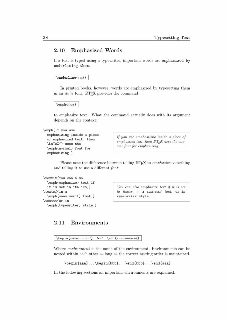
38 Typesetting Text

2.10 Emphasized Words

If a text is typed using a typewriter, important words are emphasized byunderlining them.

\underlinetext

In printed books, however, words are emphasized by typesetting themin an italic font. LATEX provides the command

\emphtext

to emphasize text. What the command actually does with its argumentdepends on the context:

\emphIf you useemphasizing inside a pieceof emphasized text, then\LaTeX uses the\emphnormal font foremphasizing.

If you use emphasizing inside a piece ofemphasized text, then LATEX uses the nor-mal font for emphasizing.

Please note the difference between telling LATEX to emphasize somethingand telling it to use a different font:

\textitYou can also\emphemphasize text ifit is set in italics,

\textsfin a\emphsans-serif font,

\textttor in\emphtypewriter style.

You can also emphasize text if it is setin italics, in a sans-serif font, or intypewriter style.

2.11 Environments

\beginenvironment text \endenvironment

Where environment is the name of the environment. Environments can benested within each other as long as the correct nesting order is maintained.

\beginaaa...\beginbbb...\endbbb...\endaaa

In the following sections all important environments are explained.

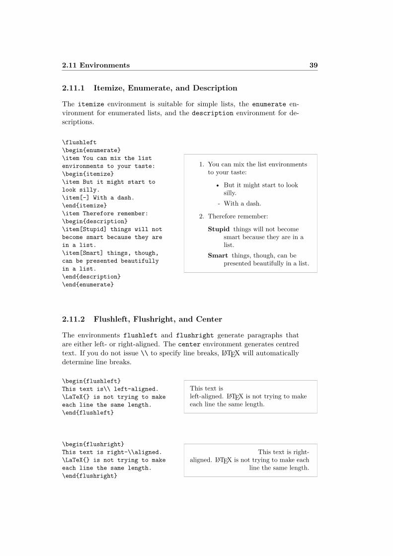
2.11 Environments 39

2.11.1 Itemize, Enumerate, and Description

The itemize environment is suitable for simple lists, the enumerate en-vironment for enumerated lists, and the description environment for de-scriptions.

\flushleft\beginenumerate\item You can mix the listenvironments to your taste:\beginitemize\item But it might start tolook silly.\item[-] With a dash.\enditemize\item Therefore remember:\begindescription\item[Stupid] things will notbecome smart because they arein a list.\item[Smart] things, though,can be presented beautifullyin a list.\enddescription\endenumerate

1. You can mix the list environmentsto your taste:

• But it might start to looksilly.

- With a dash.

2. Therefore remember:

Stupid things will not becomesmart because they are in alist.

Smart things, though, can bepresented beautifully in a list.

2.11.2 Flushleft, Flushright, and Center

The environments flushleft and flushright generate paragraphs thatare either left- or right-aligned. The center environment generates centredtext. If you do not issue \\ to specify line breaks, LATEX will automaticallydetermine line breaks.

\beginflushleftThis text is\\ left-aligned.\LaTeX is not trying to makeeach line the same length.\endflushleft

This text isleft-aligned. LATEX is not trying to makeeach line the same length.

\beginflushrightThis text is right-\\aligned.\LaTeX is not trying to makeeach line the same length.\endflushright

This text is right-aligned. LATEX is not trying to make each

line the same length.

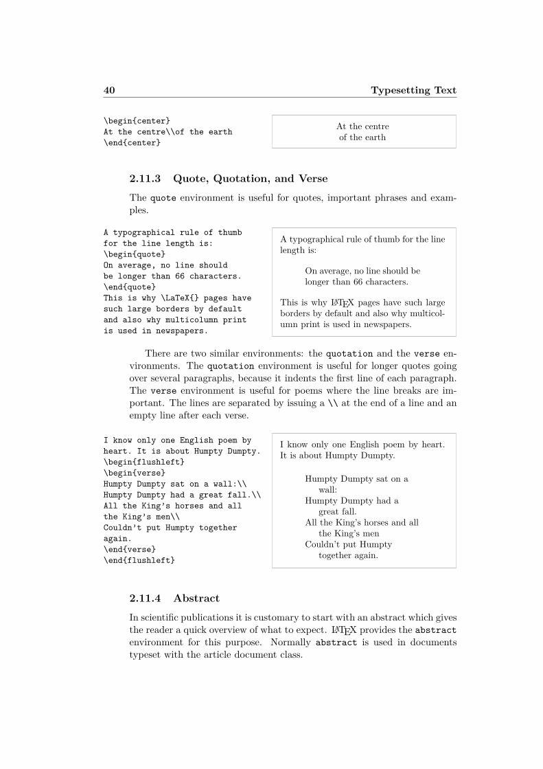
40 Typesetting Text

\begincenterAt the centre\\of the earth\endcenter

At the centreof the earth

2.11.3 Quote, Quotation, and Verse

The quote environment is useful for quotes, important phrases and exam-ples.

A typographical rule of thumbfor the line length is:\beginquoteOn average, no line shouldbe longer than 66 characters.\endquoteThis is why \LaTeX pages havesuch large borders by defaultand also why multicolumn printis used in newspapers.

A typographical rule of thumb for the linelength is:

On average, no line should belonger than 66 characters.

This is why LATEX pages have such largeborders by default and also why multicol-umn print is used in newspapers.

There are two similar environments: the quotation and the verse en-vironments. The quotation environment is useful for longer quotes goingover several paragraphs, because it indents the first line of each paragraph.The verse environment is useful for poems where the line breaks are im-portant. The lines are separated by issuing a \\ at the end of a line and anempty line after each verse.

I know only one English poem byheart. It is about Humpty Dumpty.\beginflushleft\beginverseHumpty Dumpty sat on a wall:\\Humpty Dumpty had a great fall.\\All the King’s horses and allthe King’s men\\Couldn’t put Humpty togetheragain.\endverse\endflushleft

I know only one English poem by heart.It is about Humpty Dumpty.

Humpty Dumpty sat on awall:

Humpty Dumpty had agreat fall.

All the King’s horses and allthe King’s men

Couldn’t put Humptytogether again.

2.11.4 Abstract

In scientific publications it is customary to start with an abstract which givesthe reader a quick overview of what to expect. LATEX provides the abstractenvironment for this purpose. Normally abstract is used in documentstypeset with the article document class.

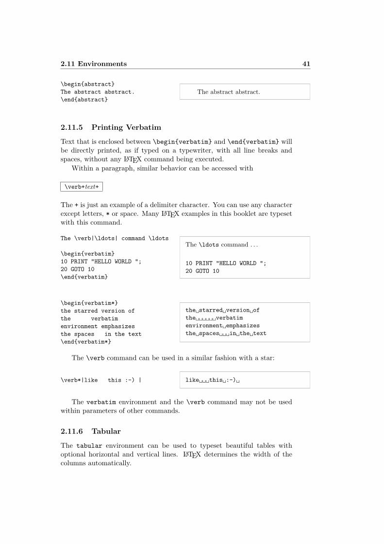
2.11 Environments 41

\beginabstractThe abstract abstract.\endabstract

The abstract abstract.

2.11.5 Printing Verbatim

Text that is enclosed between \beginverbatim and \endverbatim willbe directly printed, as if typed on a typewriter, with all line breaks andspaces, without any LATEX command being executed.

Within a paragraph, similar behavior can be accessed with

\verb+text+

The + is just an example of a delimiter character. You can use any characterexcept letters, * or space. Many LATEX examples in this booklet are typesetwith this command.

The \verb|\ldots| command \ldots

\beginverbatim10 PRINT "HELLO WORLD ";20 GOTO 10\endverbatim

The \ldots command . . .

10 PRINT "HELLO WORLD ";20 GOTO 10

\beginverbatim*the starred version ofthe verbatimenvironment emphasizesthe spaces in the text\endverbatim*

the starred version ofthe verbatimenvironment emphasizesthe spaces in the text

The \verb command can be used in a similar fashion with a star:

\verb*|like this :-) | like this :-)

The verbatim environment and the \verb command may not be usedwithin parameters of other commands.

2.11.6 Tabular

The tabular environment can be used to typeset beautiful tables withoptional horizontal and vertical lines. LATEX determines the width of thecolumns automatically.

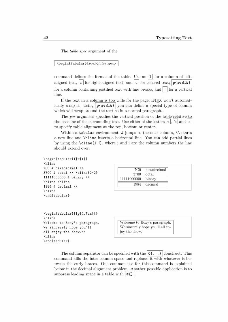
42 Typesetting Text

The table spec argument of the

\begintabular[pos]table spec

command defines the format of the table. Use an l for a column of left-aligned text, r for right-aligned text, and c for centred text; pwidth

for a column containing justified text with line breaks, and | for a verticalline.

If the text in a column is too wide for the page, LATEX won’t automat-ically wrap it. Using pwidth you can define a special type of columnwhich will wrap-around the text as in a normal paragraph.

The pos argument specifies the vertical position of the table relative tothe baseline of the surrounding text. Use either of the letters t , b and cto specify table alignment at the top, bottom or center.

Within a tabular environment, & jumps to the next column, \\ startsa new line and \hline inserts a horizontal line. You can add partial linesby using the \clinej-i, where j and i are the column numbers the lineshould extend over.

\begintabular|r|l|\hline7C0 & hexadecimal \\3700 & octal \\ \cline2-211111000000 & binary \\\hline \hline1984 & decimal \\\hline\endtabular

7C0 hexadecimal3700 octal

11111000000 binary1984 decimal

\begintabular|p4.7cm|\hlineWelcome to Boxy’s paragraph.We sincerely hope you’llall enjoy the show.\\\hline\endtabular

Welcome to Boxy’s paragraph.We sincerely hope you’ll all en-joy the show.

The column separator can be specified with the @... construct. Thiscommand kills the inter-column space and replaces it with whatever is be-tween the curly braces. One common use for this command is explainedbelow in the decimal alignment problem. Another possible application is tosuppress leading space in a table with @ .

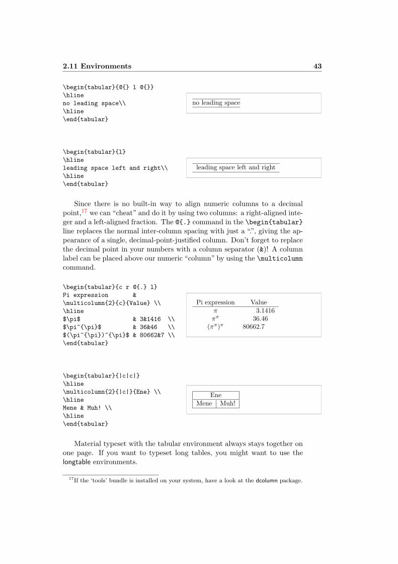
2.11 Environments 43

\begintabular@ l @\hlineno leading space\\\hline\endtabular

no leading space

\begintabularl\hlineleading space left and right\\\hline\endtabular

leading space left and right

Since there is no built-in way to align numeric columns to a decimalpoint,17 we can “cheat” and do it by using two columns: a right-aligned inte-ger and a left-aligned fraction. The @. command in the \begintabularline replaces the normal inter-column spacing with just a “.”, giving the ap-pearance of a single, decimal-point-justified column. Don’t forget to replacethe decimal point in your numbers with a column separator (&)! A columnlabel can be placed above our numeric “column” by using the \multicolumncommand.

\begintabularc r @. lPi expression &\multicolumn2cValue \\\hline$\pi$ & 3&1416 \\$\pi^\pi$ & 36&46 \\$(\pi^\pi)^\pi$ & 80662&7 \\\endtabular

Pi expression Valueπ 3.1416ππ 36.46

(ππ)π 80662.7

\begintabular|c|c|\hline\multicolumn2|c|Ene \\\hlineMene & Muh! \\\hline\endtabular

EneMene Muh!

Material typeset with the tabular environment always stays together onone page. If you want to typeset long tables, you might want to use thelongtable environments.

17If the ‘tools’ bundle is installed on your system, have a look at the dcolumn package.

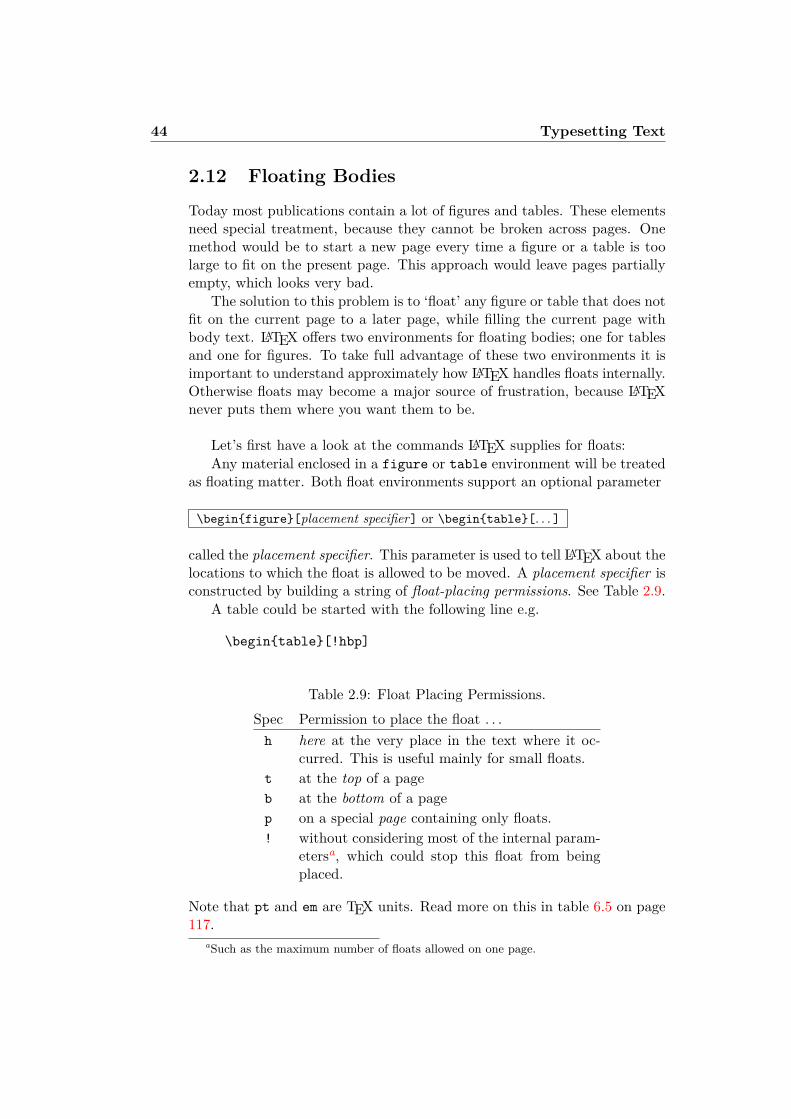
44 Typesetting Text

2.12 Floating Bodies

Today most publications contain a lot of figures and tables. These elementsneed special treatment, because they cannot be broken across pages. Onemethod would be to start a new page every time a figure or a table is toolarge to fit on the present page. This approach would leave pages partiallyempty, which looks very bad.

The solution to this problem is to ‘float’ any figure or table that does notfit on the current page to a later page, while filling the current page withbody text. LATEX offers two environments for floating bodies; one for tablesand one for figures. To take full advantage of these two environments it isimportant to understand approximately how LATEX handles floats internally.Otherwise floats may become a major source of frustration, because LATEXnever puts them where you want them to be.

Let’s first have a look at the commands LATEX supplies for floats:Any material enclosed in a figure or table environment will be treated

as floating matter. Both float environments support an optional parameter

\beginfigure[placement specifier] or \begintable[. . . ]

called the placement specifier. This parameter is used to tell LATEX about thelocations to which the float is allowed to be moved. A placement specifier isconstructed by building a string of float-placing permissions. See Table 2.9.

A table could be started with the following line e.g.

\begintable[!hbp]

Table 2.9: Float Placing Permissions.Spec Permission to place the float . . .h here at the very place in the text where it oc-

curred. This is useful mainly for small floats.t at the top of a pageb at the bottom of a pagep on a special page containing only floats.! without considering most of the internal param-

etersa, which could stop this float from beingplaced.

Note that pt and em are TEX units. Read more on this in table 6.5 on page117.

aSuch as the maximum number of floats allowed on one page.

2.12 Floating Bodies 45

The placement specifier [!hbp] allows LATEX to place the table right here(h) or at the bottom (b) of some page or on a special floats page (p), andall this even if it does not look that good (!). If no placement specifier isgiven, the standard classes assume [tbp].

LATEX will place every float it encounters according to the placementspecifier supplied by the author. If a float cannot be placed on the currentpage it is deferred either to the figures or the tables queue.18 When a newpage is started, LATEX first checks if it is possible to fill a special ‘float’page with floats from the queues. If this is not possible, the first float oneach queue is treated as if it had just occurred in the text: LATEX triesagain to place it according to its respective placement specifiers (except ‘h,’which is no longer possible). Any new floats occurring in the text get placedinto the appropriate queues. LATEX strictly maintains the original order ofappearance for each type of float. That’s why a figure that cannot be placedpushes all further figures to the end of the document. Therefore:

If LATEX is not placing the floats as you expected, it is often onlyone float jamming one of the two float queues.

While it is possible to give LATEX single-location placement specifiers,this causes problems. If the float does not fit in the location specified itbecomes stuck, blocking subsequent floats. In particular, you should never,ever use the [h] option—it is so bad that in more recent versions of LATEX,it is automatically replaced by [ht].

Having explained the difficult bit, there are some more things to mentionabout the table and figure environments. With the

\captioncaption text

command, you can define a caption for the float. A running number andthe string “Figure” or “Table” will be added by LATEX.

The two commands

\listoffigures and \listoftables

operate analogously to the \tableofcontents command, printing a list offigures or tables, respectively. These lists will display the whole caption,so if you tend to use long captions you must have a shorter version of thecaption for the lists. This is accomplished by entering the short version inbrackets after the \caption command.

\caption[Short]LLLLLoooooonnnnnggggg

18These are FIFO—‘first in first out’—queues!

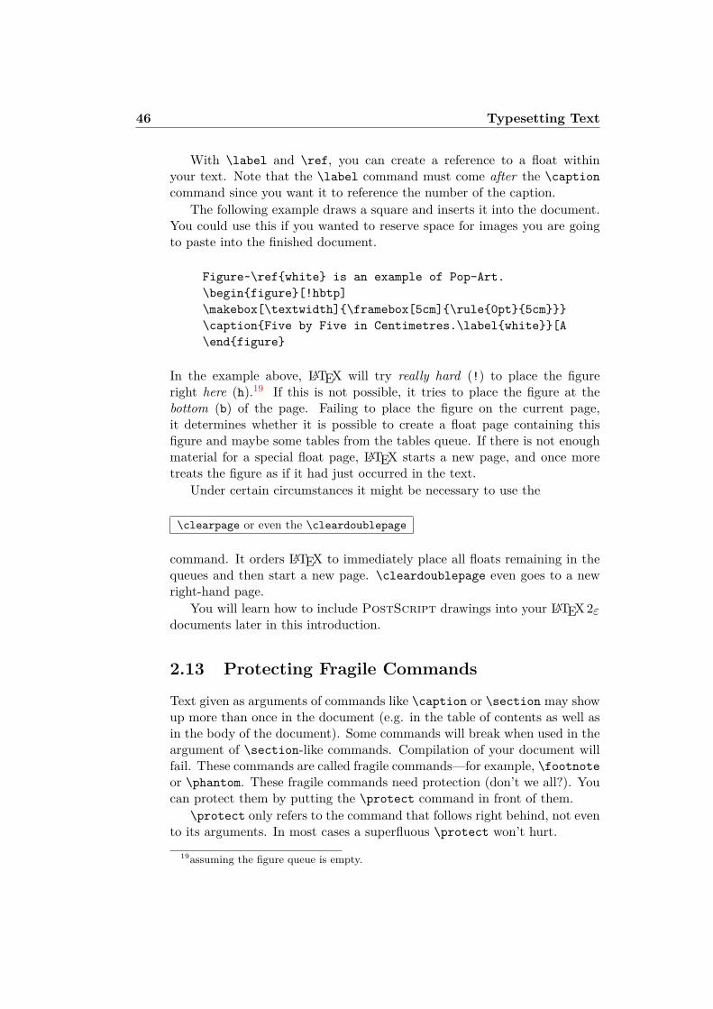
46 Typesetting Text

With \label and \ref, you can create a reference to a float withinyour text. Note that the \label command must come after the \captioncommand since you want it to reference the number of the caption.

The following example draws a square and inserts it into the document.You could use this if you wanted to reserve space for images you are goingto paste into the finished document.

Figure~\refwhite is an example of Pop-Art.\beginfigure[!hbtp]\makebox[\textwidth]\framebox[5cm]\rule0pt5cm\captionFive by Five in Centimetres.\labelwhite[A\endfigure

In the example above, LATEX will try really hard (!) to place the figureright here (h).19 If this is not possible, it tries to place the figure at thebottom (b) of the page. Failing to place the figure on the current page,it determines whether it is possible to create a float page containing thisfigure and maybe some tables from the tables queue. If there is not enoughmaterial for a special float page, LATEX starts a new page, and once moretreats the figure as if it had just occurred in the text.

Under certain circumstances it might be necessary to use the

\clearpage or even the \cleardoublepage

command. It orders LATEX to immediately place all floats remaining in thequeues and then start a new page. \cleardoublepage even goes to a newright-hand page.

You will learn how to include PostScript drawings into your LATEX2εdocuments later in this introduction.

2.13 Protecting Fragile Commands

Text given as arguments of commands like \caption or \section may showup more than once in the document (e.g. in the table of contents as well asin the body of the document). Some commands will break when used in theargument of \section-like commands. Compilation of your document willfail. These commands are called fragile commands—for example, \footnoteor \phantom. These fragile commands need protection (don’t we all?). Youcan protect them by putting the \protect command in front of them.

\protect only refers to the command that follows right behind, not evento its arguments. In most cases a superfluous \protect won’t hurt.

19assuming the figure queue is empty.

2.13 Protecting Fragile Commands 47

\sectionI am considerate\protect\footnoteand protect my footnotes

Chapter 3

Typesetting MathematicalFormulae

Now you are ready! In this chapter, we will attack the main strength of TEX:mathematical typesetting. But be warned, this chapter only scratches the sur-face. While the things explained here are sufficient for many people, don’tdespair if you can’t find a solution to your mathematical typesetting needs here.It is highly likely that your problem is addressed in AMS-LATEX.

3.1 The AMS-LATEX bundleIf you want to typeset (advanced) mathematics, you should use AMS-LATEX.The AMS-LATEX bundle is a collection of packages and classes for mathe-matical typesetting. We will mostly deal with the amsmath package which isa part of the bundle. AMS-LATEX is produced by The American Mathemat-ical Society and it is used extensively for mathematical typesetting. LATEXitself does provide some basic features and environments for mathematics,but they are limited (or maybe it’s the other way around: AMS-LATEX isunlimited!) and in some cases inconsistent.

AMS-LATEX is a part of the required distribution and is provided with allrecent LATEX distributions.1 In this chapter, we assume amsmath is loadedin the preamble; \usepackageamsmath.

3.2 Single EquationsThere two ways to typeset mathematical formulae: in-line within a para-graph (text style), or the paragraph can be broken to typeset it separately(display style). Mathematical equations within a paragraph is entered be-tween between $ and $:

1If yours is missing it, go to CTAN:macros/latex/required/amslatex.

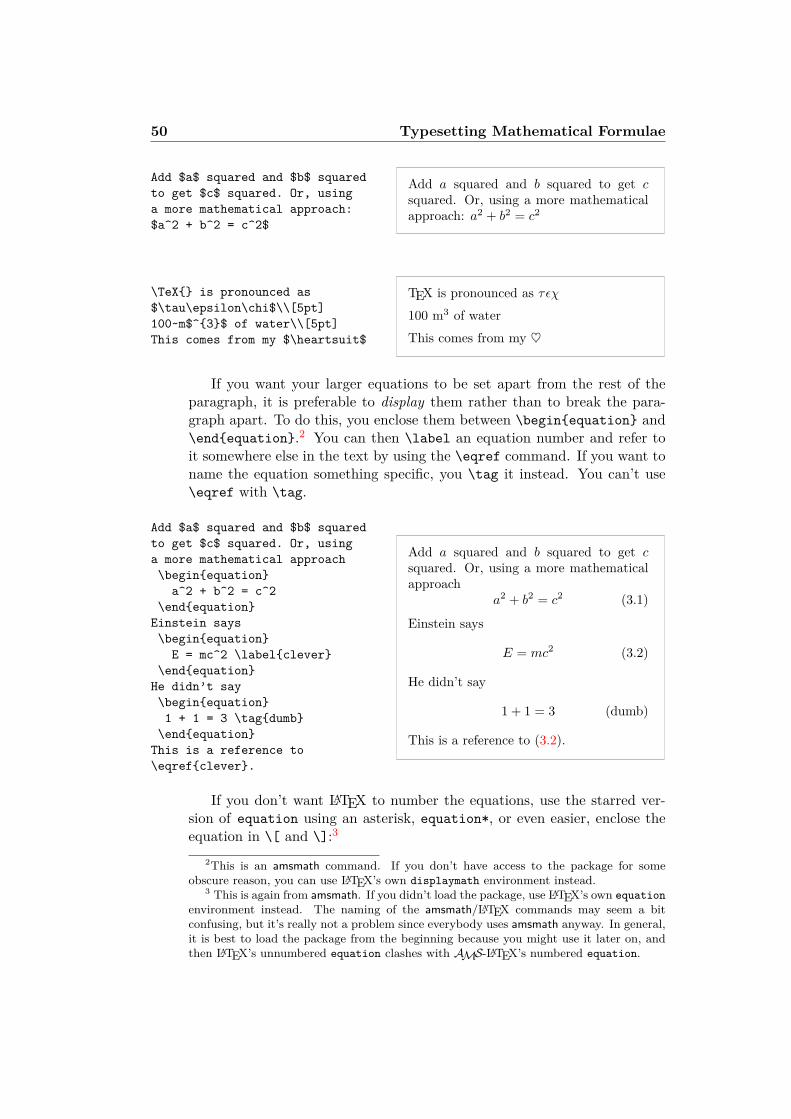
50 Typesetting Mathematical Formulae

Add $a$ squared and $b$ squaredto get $c$ squared. Or, usinga more mathematical approach:$a^2 + b^2 = c^2$

Add a squared and b squared to get csquared. Or, using a more mathematicalapproach: a2 + b2 = c2

\TeX is pronounced as$\tau\epsilon\chi$\\[5pt]100~m$^3$ of water\\[5pt]This comes from my $\heartsuit$

TEX is pronounced as τεχ100 m3 of waterThis comes from my ♥

If you want your larger equations to be set apart from the rest of theparagraph, it is preferable to display them rather than to break the para-graph apart. To do this, you enclose them between \beginequation and\endequation.2 You can then \label an equation number and refer toit somewhere else in the text by using the \eqref command. If you want toname the equation something specific, you \tag it instead. You can’t use\eqref with \tag.

Add $a$ squared and $b$ squaredto get $c$ squared. Or, usinga more mathematical approach\beginequationa^2 + b^2 = c^2

\endequationEinstein says\beginequationE = mc^2 \labelclever

\endequationHe didn’t say\beginequation1 + 1 = 3 \tagdumb

\endequationThis is a reference to\eqrefclever.

Add a squared and b squared to get csquared. Or, using a more mathematicalapproach

a2 + b2 = c2 (3.1)

Einstein says

E = mc2 (3.2)

He didn’t say

1 + 1 = 3 (dumb)

This is a reference to (3.2).

If you don’t want LATEX to number the equations, use the starred ver-sion of equation using an asterisk, equation*, or even easier, enclose theequation in \[ and \]:3

2This is an amsmath command. If you don’t have access to the package for someobscure reason, you can use LATEX’s own displaymath environment instead.

3 This is again from amsmath. If you didn’t load the package, use LATEX’s own equationenvironment instead. The naming of the amsmath/LATEX commands may seem a bitconfusing, but it’s really not a problem since everybody uses amsmath anyway. In general,it is best to load the package from the beginning because you might use it later on, andthen LATEX’s unnumbered equation clashes with AMS-LATEX’s numbered equation.

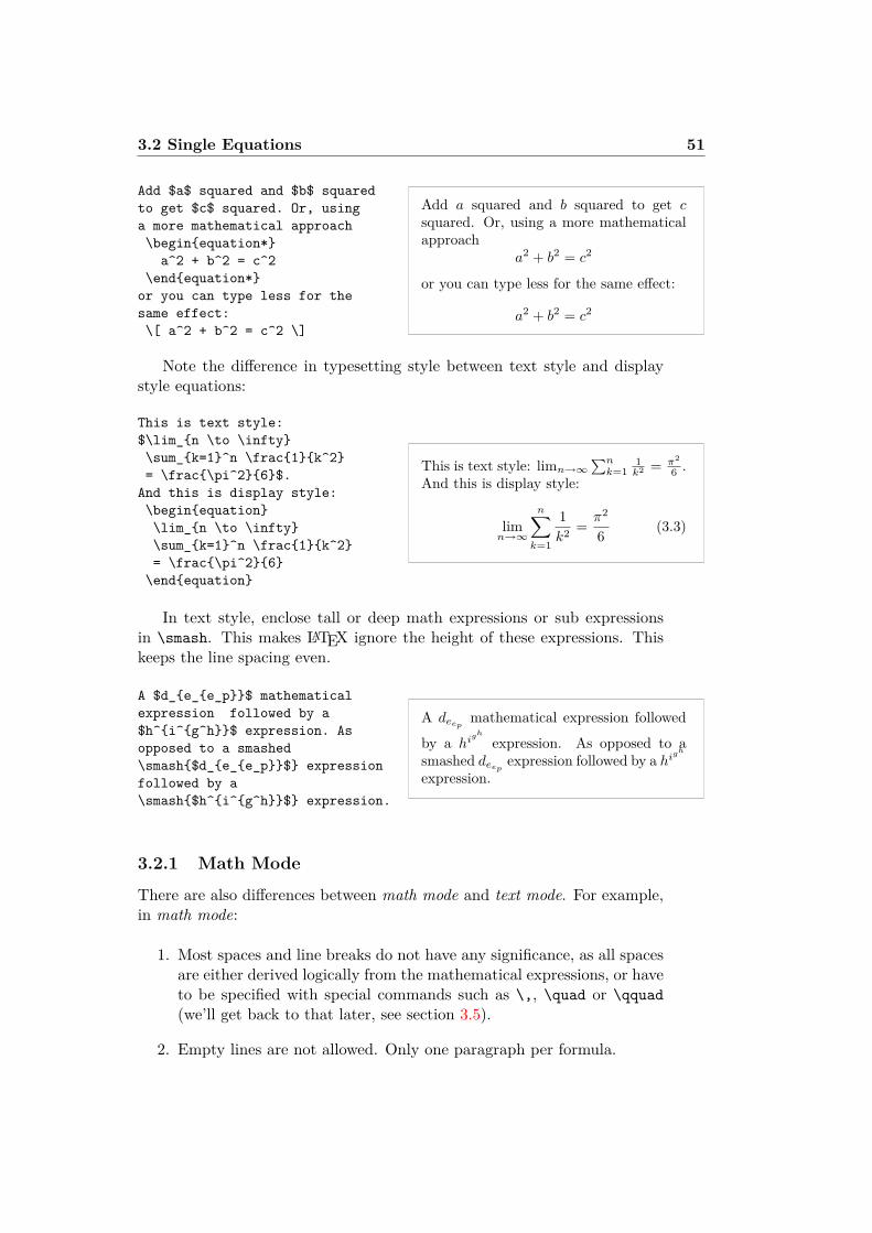
3.2 Single Equations 51

Add $a$ squared and $b$ squaredto get $c$ squared. Or, usinga more mathematical approach\beginequation*a^2 + b^2 = c^2

\endequation*or you can type less for thesame effect:\[ a^2 + b^2 = c^2 \]

Add a squared and b squared to get csquared. Or, using a more mathematicalapproach

a2 + b2 = c2

or you can type less for the same effect:

a2 + b2 = c2

Note the difference in typesetting style between text style and displaystyle equations:

This is text style:$\lim_n \to \infty\sum_k=1^n \frac1k^2= \frac\pi^26$.And this is display style:\beginequation\lim_n \to \infty\sum_k=1^n \frac1k^2= \frac\pi^26

\endequation

This is text style: limn→∞∑nk=1

1k2 = π2

6 .And this is display style:

limn→∞

n∑k=1

1k2 = π2

6(3.3)

In text style, enclose tall or deep math expressions or sub expressionsin \smash. This makes LATEX ignore the height of these expressions. Thiskeeps the line spacing even.

A $d_e_e_p$ mathematicalexpression followed by a$h^i^g^h$ expression. Asopposed to a smashed\smash$d_e_e_p$ expressionfollowed by a\smash$h^i^g^h$ expression.

A deep mathematical expression followed

by a high expression. As opposed to a

smashed deep expression followed by a high

expression.

3.2.1 Math Mode

There are also differences between math mode and text mode. For example,in math mode:

1. Most spaces and line breaks do not have any significance, as all spacesare either derived logically from the mathematical expressions, or haveto be specified with special commands such as \,, \quad or \qquad(we’ll get back to that later, see section 3.5).

2. Empty lines are not allowed. Only one paragraph per formula.

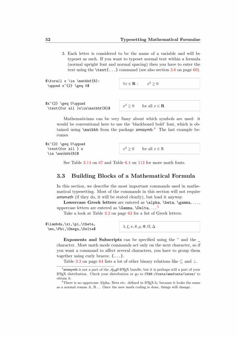
52 Typesetting Mathematical Formulae

3. Each letter is considered to be the name of a variable and will betypeset as such. If you want to typeset normal text within a formula(normal upright font and normal spacing) then you have to enter thetext using the \text... command (see also section 3.6 on page 60).

$\forall x \in \mathbfR:\qquad x^2 \geq 0$ ∀x ∈ R : x2 ≥ 0

$x^2 \geq 0\qquad\textfor all x\in\mathbfR$ x2 ≥ 0 for all x ∈ R

Mathematicians can be very fussy about which symbols are used: itwould be conventional here to use the ‘blackboard bold’ font, which is ob-tained using \mathbb from the package amssymb.4 The last example be-comes

$x^2 \geq 0\qquad\textfor all x\in \mathbbR$

x2 ≥ 0 for all x ∈ R

See Table 3.14 on 67 and Table 6.4 on 113 for more math fonts.

3.3 Building Blocks of a Mathematical FormulaIn this section, we describe the most important commands used in mathe-matical typesetting. Most of the commands in this section will not requireamsmath (if they do, it will be stated clearly), but load it anyway.

Lowercase Greek letters are entered as \alpha, \beta, \gamma, . . . ,uppercase letters are entered as \Gamma, \Delta, . . . 5

Take a look at Table 3.2 on page 63 for a list of Greek letters.

$\lambda,\xi,\pi,\theta,\mu,\Phi,\Omega,\Delta$ λ, ξ, π, θ, µ,Φ,Ω,∆

Exponents and Subscripts can be specified using the ^ and the _character. Most math mode commands act only on the next character, so ifyou want a command to affect several characters, you have to group themtogether using curly braces: ....

Table 3.3 on page 64 lists a lot of other binary relations like ⊆ and ⊥.4amssymb is not a part of the AMS-LATEX bundle, but it is perhaps still a part of your

LATEX distribution. Check your distribution or go to CTAN:/fonts/amsfonts/latex/ toobtain it.

5There is no uppercase Alpha, Beta etc. defined in LATEX2ε because it looks the sameas a normal roman A, B. . . Once the new math coding is done, things will change.

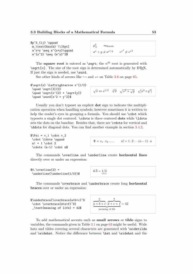
3.3 Building Blocks of a Mathematical Formula 53

$p^3_ij \qquadm_\textKnuth \\[5pt]a^x+y \neq a^x+y\qquade^x^2 \neq e^x^2$

p3ij mKnuth

ax + y 6= ax+y ex2 6= ex2

The square root is entered as \sqrt; the nth root is generated with\sqrt[n]. The size of the root sign is determined automatically by LATEX.If just the sign is needed, use \surd.

See other kinds of arrows like → and on Table 3.6 on page 65.

$\sqrtx \Leftrightarrow x^1/2\quad \sqrt[3]2\quad \sqrtx^2 + \sqrty\quad \surd[x^2 + y^2]$

√x⇔ x1/2 3

√2√x2 +√y

√[x2 +y2]

Usually you don’t typeset an explicit dot sign to indicate the multipli-cation operation when handling symbols; however sometimes it is written tohelp the reader’s eyes in grouping a formula. You should use \cdot whichtypesets a single dot centered. \cdots is three centered dots while \ldotssets the dots on the baseline. Besides that, there are \vdots for vertical and\ddots for diagonal dots. You can find another example in section 3.4.2.

$\Psi = v_1 \cdot v_2\cdot \ldots \qquadn! = 1 \cdot 2\cdots (n-1) \cdot n$

Ψ = v1 · v2 · . . . n! = 1 · 2 · · · (n− 1) ·n

The commands \overline and \underline create horizontal linesdirectly over or under an expression:

$0.\overline3 =\underline\underline1/3$

0.3 = 1/3

The commands \overbrace and \underbrace create long horizontalbraces over or under an expression:

$\underbrace\overbracea+b+c^6\cdot \overbraced+e+f^9_\textmeaning of life = 42$

6︷ ︸︸ ︷a+ b+ c ·

9︷ ︸︸ ︷d+ e+ f︸ ︷︷ ︸

meaning of life

= 42

To add mathematical accents such as small arrows or tilde signs tovariables, the commands given in Table 3.1 on page 63 might be useful. Widehats and tildes covering several characters are generated with \widetildeand \widehat. Notice the difference between \hat and \widehat and the

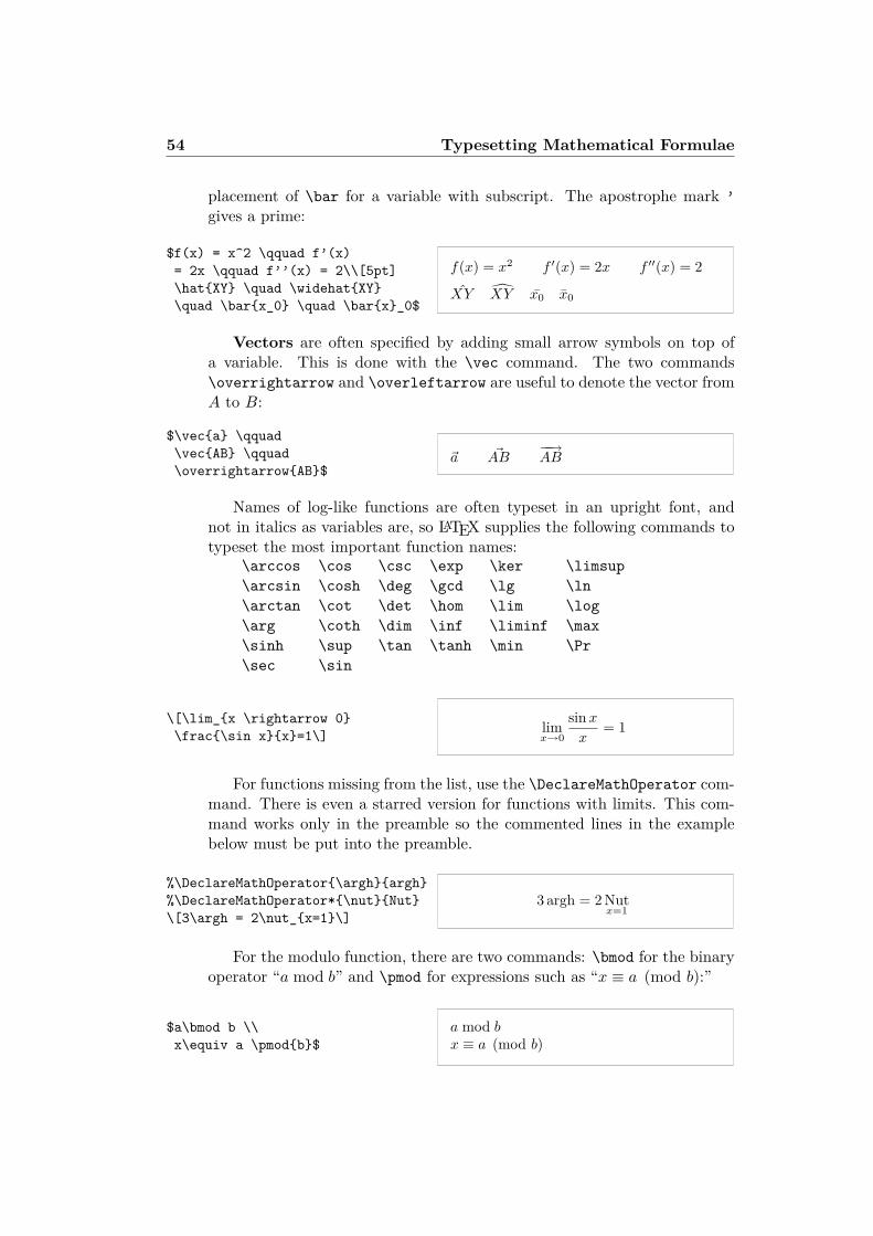
54 Typesetting Mathematical Formulae

placement of \bar for a variable with subscript. The apostrophe mark ’gives a prime:

$f(x) = x^2 \qquad f’(x)= 2x \qquad f’’(x) = 2\\[5pt]\hatXY \quad \widehatXY\quad \barx_0 \quad \barx_0$

f(x) = x2 f ′(x) = 2x f ′′(x) = 2

XY XY x0 x0

Vectors are often specified by adding small arrow symbols on top ofa variable. This is done with the \vec command. The two commands\overrightarrow and \overleftarrow are useful to denote the vector fromA to B:

$\veca \qquad\vecAB \qquad\overrightarrowAB$

~a ~AB−−→AB

Names of log-like functions are often typeset in an upright font, andnot in italics as variables are, so LATEX supplies the following commands totypeset the most important function names:

\arccos \cos \csc \exp \ker \limsup\arcsin \cosh \deg \gcd \lg \ln\arctan \cot \det \hom \lim \log\arg \coth \dim \inf \liminf \max\sinh \sup \tan \tanh \min \Pr\sec \sin

\[\lim_x \rightarrow 0\frac\sin xx=1\] lim

x→0

sin xx

= 1

For functions missing from the list, use the \DeclareMathOperator com-mand. There is even a starred version for functions with limits. This com-mand works only in the preamble so the commented lines in the examplebelow must be put into the preamble.

%\DeclareMathOperator\arghargh%\DeclareMathOperator*\nutNut\[3\argh = 2\nut_x=1\]

3 argh = 2 Nutx=1

For the modulo function, there are two commands: \bmod for the binaryoperator “a mod b” and \pmod for expressions such as “x ≡ a (mod b):”

$a\bmod b \\x\equiv a \pmodb$

a mod bx ≡ a (mod b)

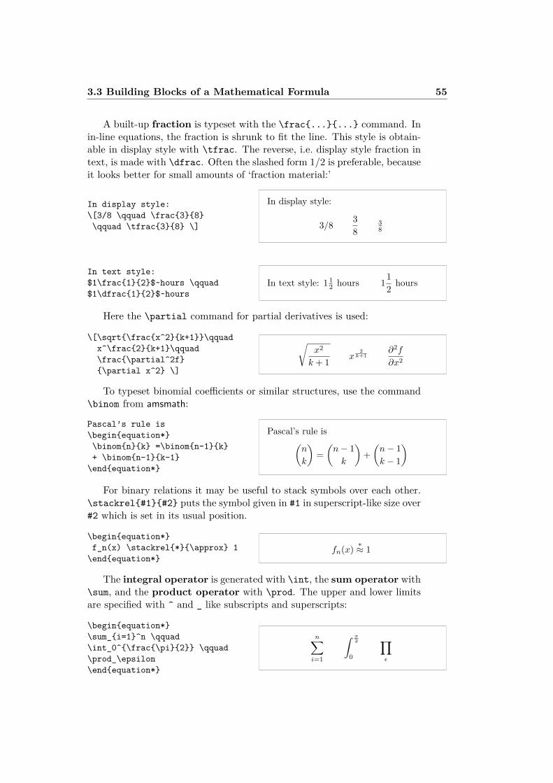
3.3 Building Blocks of a Mathematical Formula 55

A built-up fraction is typeset with the \frac...... command. Inin-line equations, the fraction is shrunk to fit the line. This style is obtain-able in display style with \tfrac. The reverse, i.e. display style fraction intext, is made with \dfrac. Often the slashed form 1/2 is preferable, becauseit looks better for small amounts of ‘fraction material:’

In display style:\[3/8 \qquad \frac38\qquad \tfrac38 \]

In display style:

3/8 38

38

In text style:$1\frac12$~hours \qquad$1\dfrac12$~hours

In text style: 1 12 hours 11

2hours

Here the \partial command for partial derivatives is used:

\[\sqrt\fracx^2k+1\qquadx^\frac2k+1\qquad\frac\partial^2f\partial x^2 \]

√x2

k + 1x

2k+1

∂2f

∂x2

To typeset binomial coefficients or similar structures, use the command\binom from amsmath:

Pascal’s rule is\beginequation*\binomnk =\binomn-1k+ \binomn-1k-1\endequation*

Pascal’s rule is(n

k

)=(n− 1k

)+(n− 1k − 1

)

For binary relations it may be useful to stack symbols over each other.\stackrel#1#2 puts the symbol given in #1 in superscript-like size over#2 which is set in its usual position.

\beginequation*f_n(x) \stackrel*\approx 1\endequation*

fn(x)∗≈ 1

The integral operator is generated with \int, the sum operator with\sum, and the product operator with \prod. The upper and lower limitsare specified with ^ and _ like subscripts and superscripts:

\beginequation*\sum_i=1^n \qquad\int_0^\frac\pi2 \qquad\prod_\epsilon\endequation*

n∑i=1

∫ π2

0

∏ε

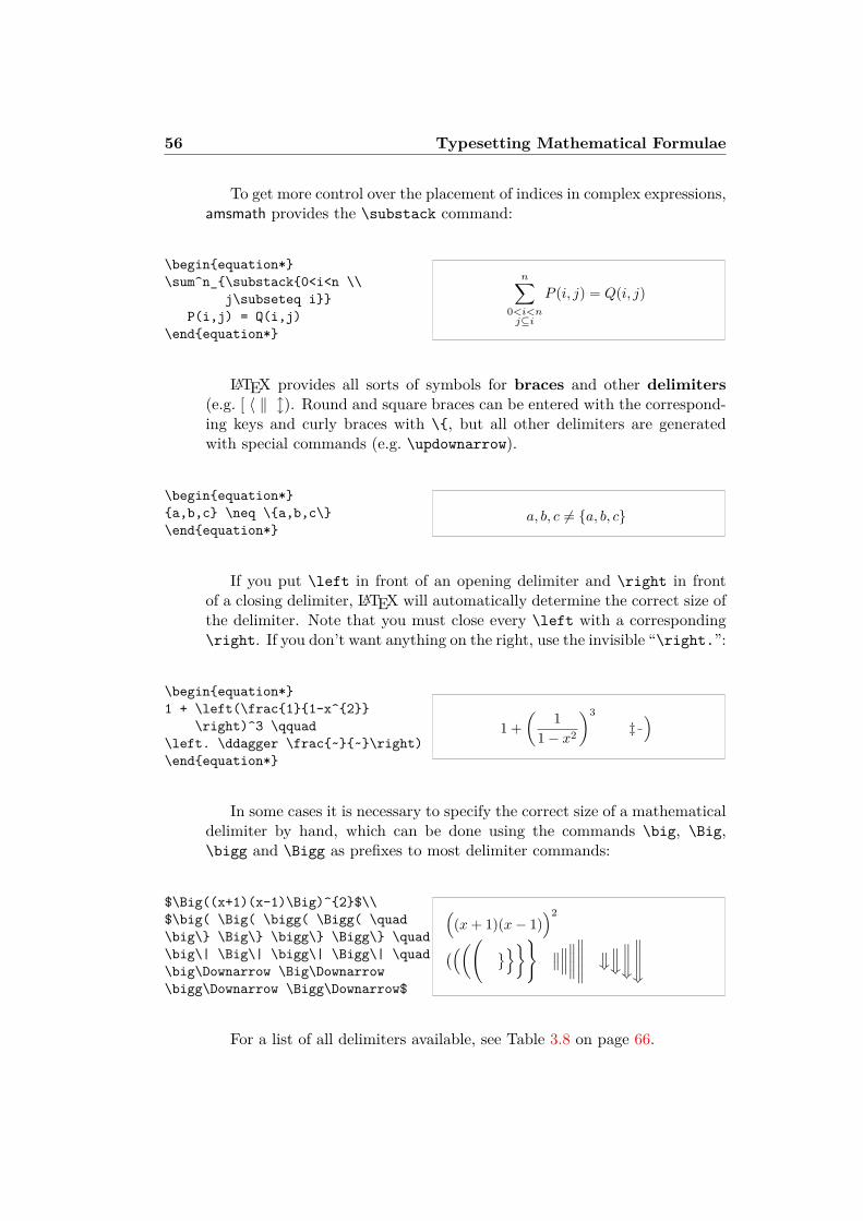
56 Typesetting Mathematical Formulae

To get more control over the placement of indices in complex expressions,amsmath provides the \substack command:

\beginequation*\sum^n_\substack0<i<n \\

j\subseteq iP(i,j) = Q(i,j)

\endequation*

n∑0<i<nj⊆i

P (i, j) = Q(i, j)

LATEX provides all sorts of symbols for braces and other delimiters(e.g. [ 〈 ‖ l). Round and square braces can be entered with the correspond-ing keys and curly braces with \, but all other delimiters are generatedwith special commands (e.g. \updownarrow).

\beginequation*a,b,c \neq \a,b,c\\endequation*

a, b, c 6= a, b, c

If you put \left in front of an opening delimiter and \right in frontof a closing delimiter, LATEX will automatically determine the correct size ofthe delimiter. Note that you must close every \left with a corresponding\right. If you don’t want anything on the right, use the invisible “\right.”:

\beginequation*1 + \left(\frac11-x^2

\right)^3 \qquad\left. \ddagger \frac~~\right)\endequation*

1 +(

11− x2

)3‡)

In some cases it is necessary to specify the correct size of a mathematicaldelimiter by hand, which can be done using the commands \big, \Big,\bigg and \Bigg as prefixes to most delimiter commands:

$\Big((x+1)(x-1)\Big)^2$\\$\big( \Big( \bigg( \Bigg( \quad\big\ \Big\ \bigg\ \Bigg\ \quad\big\| \Big\| \bigg\| \Bigg\| \quad\big\Downarrow \Big\Downarrow\bigg\Downarrow \Bigg\Downarrow$

((x+ 1)(x− 1)

)2

(((( ∥∥∥∥∥∥∥∥∥∥∥∥∥∥ wwwwww

wwww

For a list of all delimiters available, see Table 3.8 on page 66.

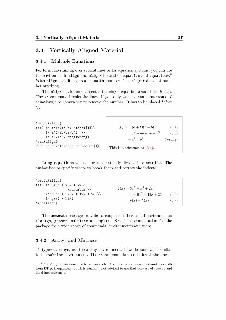
3.4 Vertically Aligned Material 57

3.4 Vertically Aligned Material

3.4.1 Multiple Equations

For formulae running over several lines or for equation systems, you can usethe environments align and align* instead of equation and equation*.6With align each line gets an equation number. The align* does not num-ber anything.

The align environments center the single equation around the & sign.The \\ command breaks the lines. If you only want to enumerate some ofequations, use \nonumber to remove the number. It has to be placed before\\:

\beginalignf(x) &= (a+b)(a-b) \label1\\

&= a^2-ab+ba-b^2 \\&= a^2+b^2 \tagwrong

\endalignThis is a reference to \eqref1.

f(x) = (a+ b)(a− b) (3.4)= a2 − ab+ ba− b2 (3.5)= a2 + b2 (wrong)

This is a reference to (3.4).

Long equations will not be automatically divided into neat bits. Theauthor has to specify where to break them and correct the indent:

\beginalignf(x) &= 3x^5 + x^4 + 2x^3

\nonumber \\&\qquad + 9x^2 + 12x + 23 \\&= g(x) - h(x)

\endalign

f(x) = 3x5 + x4 + 2x3

+ 9x2 + 12x+ 23 (3.6)= g(x)− h(x) (3.7)

The amsmath package provides a couple of other useful environments:flalign, gather, multline and split. See the documentation for thepackage for a wide range of commands, environments and more.

3.4.2 Arrays and Matrices

To typeset arrays, use the array environment. It works somewhat similarto the tabular environment. The \\ command is used to break the lines:

6The align environment is from amsmath. A similar environment without amsmathfrom LATEX is eqnarray, but it is generally not advised to use that because of spacing andlabel inconsistencies.

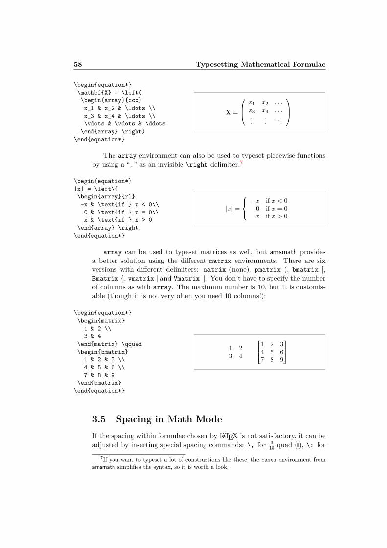
58 Typesetting Mathematical Formulae

\beginequation*\mathbfX = \left(\beginarraycccx_1 & x_2 & \ldots \\x_3 & x_4 & \ldots \\\vdots & \vdots & \ddots\endarray \right)

\endequation*

X =

x1 x2 . . .x3 x4 . . ....

.... . .

The array environment can also be used to typeset piecewise functionsby using a “.” as an invisible \right delimiter:7

\beginequation*|x| = \left\\beginarrayrl-x & \textif x < 0\\0 & \textif x = 0\\x & \textif x > 0

\endarray \right.\endequation*

|x| =

−x if x < 00 if x = 0x if x > 0

array can be used to typeset matrices as well, but amsmath providesa better solution using the different matrix environments. There are sixversions with different delimiters: matrix (none), pmatrix (, bmatrix [,Bmatrix , vmatrix | and Vmatrix ‖. You don’t have to specify the numberof columns as with array. The maximum number is 10, but it is customis-able (though it is not very often you need 10 columns!):

\beginequation*\beginmatrix1 & 2 \\3 & 4

\endmatrix \qquad\beginbmatrix1 & 2 & 3 \\4 & 5 & 6 \\7 & 8 & 9

\endbmatrix\endequation*

1 23 4

1 2 34 5 67 8 9

3.5 Spacing in Math Mode

If the spacing within formulae chosen by LATEX is not satisfactory, it can beadjusted by inserting special spacing commands: \, for 3

18 quad ( ), \: for

7If you want to typeset a lot of constructions like these, the cases environment fromamsmath simplifies the syntax, so it is worth a look.

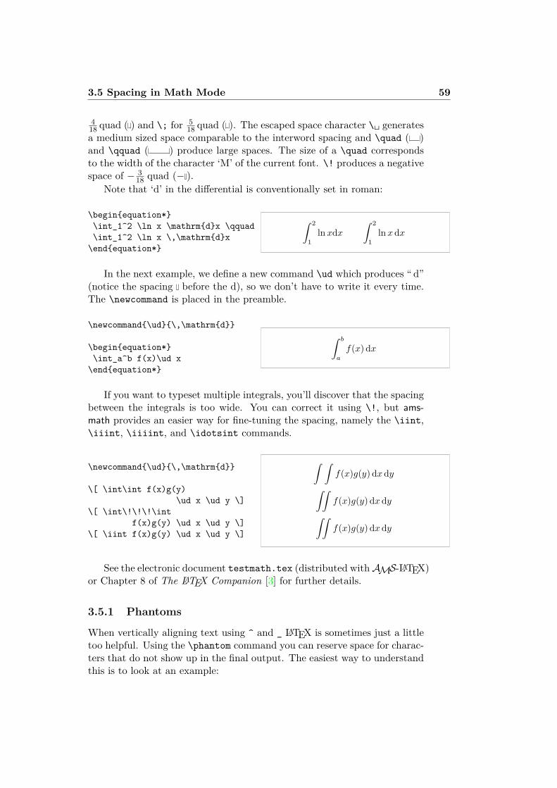
3.5 Spacing in Math Mode 59

418 quad ( ) and \; for 5

18 quad ( ). The escaped space character \ generatesa medium sized space comparable to the interword spacing and \quad ( )and \qquad ( ) produce large spaces. The size of a \quad correspondsto the width of the character ‘M’ of the current font. \! produces a negativespace of − 3

18 quad (− ).Note that ‘d’ in the differential is conventionally set in roman:

\beginequation*\int_1^2 \ln x \mathrmdx \qquad\int_1^2 \ln x \,\mathrmdx\endequation*

∫ 2

1ln xdx

∫ 2

1ln x dx

In the next example, we define a new command \ud which produces “ d”(notice the spacing before the d), so we don’t have to write it every time.The \newcommand is placed in the preamble.

\newcommand\ud\,\mathrmd

\beginequation*\int_a^b f(x)\ud x\endequation*

∫ b

a

f(x) dx

If you want to typeset multiple integrals, you’ll discover that the spacingbetween the integrals is too wide. You can correct it using \!, but ams-math provides an easier way for fine-tuning the spacing, namely the \iint,\iiint, \iiiint, and \idotsint commands.

\newcommand\ud\,\mathrmd

\[ \int\int f(x)g(y)\ud x \ud y \]

\[ \int\!\!\!\intf(x)g(y) \ud x \ud y \]

\[ \iint f(x)g(y) \ud x \ud y \]

∫ ∫f(x)g(y) dx dy∫∫f(x)g(y) dx dy∫∫f(x)g(y) dx dy

See the electronic document testmath.tex (distributed withAMS-LATEX)or Chapter 8 of The LATEX Companion [3] for further details.

3.5.1 Phantoms

When vertically aligning text using ^ and _ LATEX is sometimes just a littletoo helpful. Using the \phantom command you can reserve space for charac-ters that do not show up in the final output. The easiest way to understandthis is to look at an example:

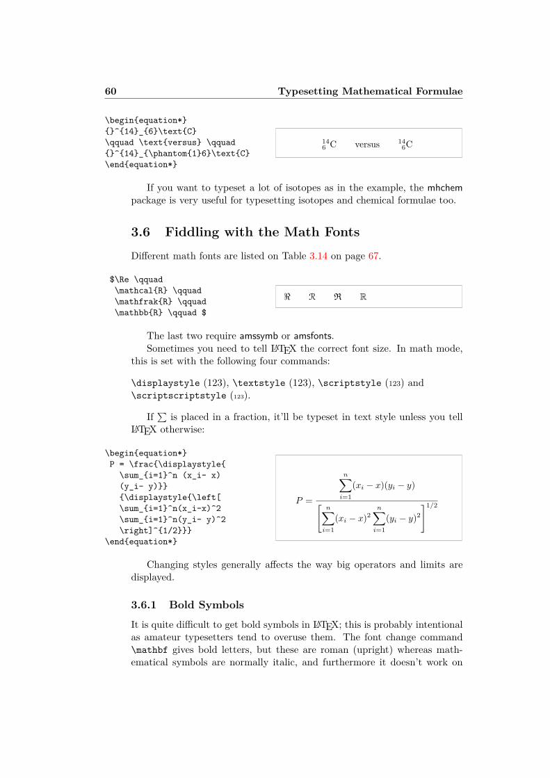
60 Typesetting Mathematical Formulae

\beginequation*^14_6\textC\qquad \textversus \qquad^14_\phantom16\textC\endequation*

146 C versus 14

6C

If you want to typeset a lot of isotopes as in the example, the mhchempackage is very useful for typesetting isotopes and chemical formulae too.

3.6 Fiddling with the Math Fonts

Different math fonts are listed on Table 3.14 on page 67.

$\Re \qquad\mathcalR \qquad\mathfrakR \qquad\mathbbR \qquad $

< R R R

The last two require amssymb or amsfonts.Sometimes you need to tell LATEX the correct font size. In math mode,

this is set with the following four commands:

\displaystyle (123), \textstyle (123), \scriptstyle (123) and\scriptscriptstyle (123).

If∑

is placed in a fraction, it’ll be typeset in text style unless you tellLATEX otherwise:

\beginequation*P = \frac\displaystyle

\sum_i=1^n (x_i- x)(y_i- y)\displaystyle\left[\sum_i=1^n(x_i-x)^2\sum_i=1^n(y_i- y)^2\right]^1/2

\endequation*

P =

n∑i=1

(xi − x)(yi − y)[n∑i=1

(xi − x)2n∑i=1

(yi − y)2

]1/2

Changing styles generally affects the way big operators and limits aredisplayed.

3.6.1 Bold Symbols

It is quite difficult to get bold symbols in LATEX; this is probably intentionalas amateur typesetters tend to overuse them. The font change command\mathbf gives bold letters, but these are roman (upright) whereas math-ematical symbols are normally italic, and furthermore it doesn’t work on

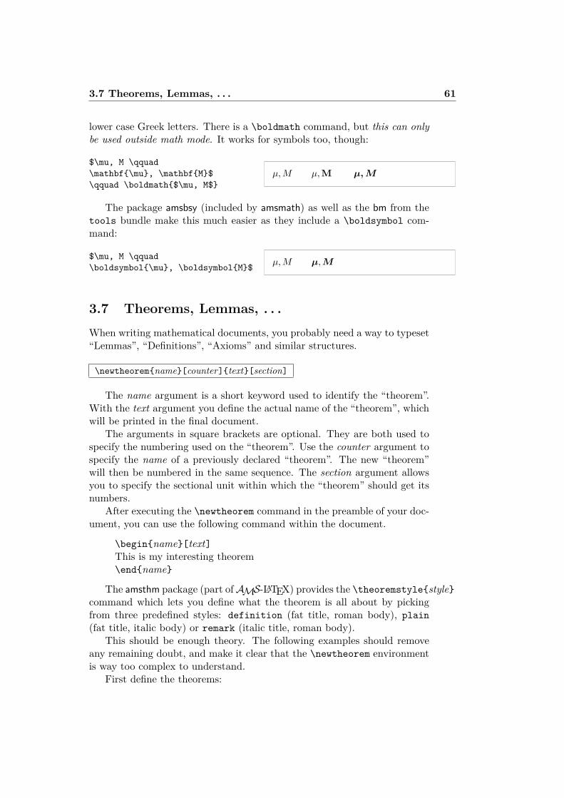
3.7 Theorems, Lemmas, . . . 61

lower case Greek letters. There is a \boldmath command, but this can onlybe used outside math mode. It works for symbols too, though:

$\mu, M \qquad\mathbf\mu, \mathbfM$\qquad \boldmath$\mu, M$

µ,M µ,M µ,M

The package amsbsy (included by amsmath) as well as the bm from thetools bundle make this much easier as they include a \boldsymbol com-mand:

$\mu, M \qquad\boldsymbol\mu, \boldsymbolM$ µ,M µ,M

3.7 Theorems, Lemmas, . . .When writing mathematical documents, you probably need a way to typeset“Lemmas”, “Definitions”, “Axioms” and similar structures.

\newtheoremname[counter]text[section]

The name argument is a short keyword used to identify the “theorem”.With the text argument you define the actual name of the “theorem”, whichwill be printed in the final document.

The arguments in square brackets are optional. They are both used tospecify the numbering used on the “theorem”. Use the counter argument tospecify the name of a previously declared “theorem”. The new “theorem”will then be numbered in the same sequence. The section argument allowsyou to specify the sectional unit within which the “theorem” should get itsnumbers.

After executing the \newtheorem command in the preamble of your doc-ument, you can use the following command within the document.

\beginname[text]This is my interesting theorem\endname

The amsthm package (part ofAMS-LATEX) provides the \theoremstylestylecommand which lets you define what the theorem is all about by pickingfrom three predefined styles: definition (fat title, roman body), plain(fat title, italic body) or remark (italic title, roman body).

This should be enough theory. The following examples should removeany remaining doubt, and make it clear that the \newtheorem environmentis way too complex to understand.

First define the theorems:

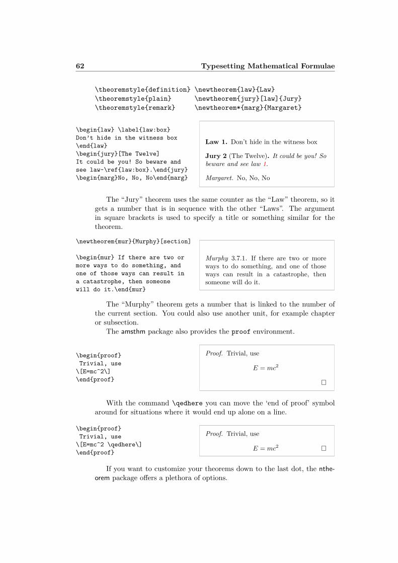
62 Typesetting Mathematical Formulae

\theoremstyledefinition \newtheoremlawLaw\theoremstyleplain \newtheoremjury[law]Jury\theoremstyleremark \newtheorem*margMargaret

\beginlaw \labellaw:boxDon’t hide in the witness box\endlaw\beginjury[The Twelve]It could be you! So beware andsee law~\reflaw:box.\endjury\beginmargNo, No, No\endmarg

Law 1. Don’t hide in the witness box

Jury 2 (The Twelve). It could be you! Sobeware and see law 1.

Margaret. No, No, No

The “Jury” theorem uses the same counter as the “Law” theorem, so itgets a number that is in sequence with the other “Laws”. The argumentin square brackets is used to specify a title or something similar for thetheorem.

\newtheoremmurMurphy[section]

\beginmur If there are two ormore ways to do something, andone of those ways can result ina catastrophe, then someonewill do it.\endmur

Murphy 3.7.1. If there are two or moreways to do something, and one of thoseways can result in a catastrophe, thensomeone will do it.

The “Murphy” theorem gets a number that is linked to the number ofthe current section. You could also use another unit, for example chapteror subsection.

The amsthm package also provides the proof environment.

\beginproofTrivial, use\[E=mc^2\]\endproof

Proof. Trivial, use

E = mc2

With the command \qedhere you can move the ‘end of proof’ symbolaround for situations where it would end up alone on a line.

\beginproofTrivial, use\[E=mc^2 \qedhere\]\endproof

Proof. Trivial, use

E = mc2

If you want to customize your theorems down to the last dot, the nthe-orem package offers a plethora of options.

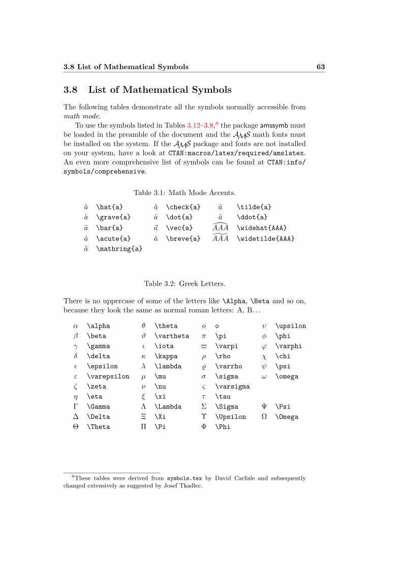
3.8 List of Mathematical Symbols 63

3.8 List of Mathematical SymbolsThe following tables demonstrate all the symbols normally accessible frommath mode.

To use the symbols listed in Tables 3.12–3.8,8 the package amssymb mustbe loaded in the preamble of the document and the AMS math fonts mustbe installed on the system. If the AMS package and fonts are not installedon your system, have a look at CTAN:macros/latex/required/amslatex.An even more comprehensive list of symbols can be found at CTAN:info/symbols/comprehensive.

Table 3.1: Math Mode Accents.

a \hata a \checka a \tildeaa \gravea a \dota a \ddotaa \bara ~a \veca AAA \widehatAAAa \acutea a \brevea AAA \widetildeAAAa \mathringa

Table 3.2: Greek Letters.

There is no uppercase of some of the letters like \Alpha, \Beta and so on,because they look the same as normal roman letters: A, B. . .

α \alpha θ \theta o o υ \upsilonβ \beta ϑ \vartheta π \pi φ \phiγ \gamma ι \iota $ \varpi ϕ \varphiδ \delta κ \kappa ρ \rho χ \chiε \epsilon λ \lambda % \varrho ψ \psiε \varepsilon µ \mu σ \sigma ω \omegaζ \zeta ν \nu ς \varsigmaη \eta ξ \xi τ \tauΓ \Gamma Λ \Lambda Σ \Sigma Ψ \Psi∆ \Delta Ξ \Xi Υ \Upsilon Ω \OmegaΘ \Theta Π \Pi Φ \Phi

8These tables were derived from symbols.tex by David Carlisle and subsequentlychanged extensively as suggested by Josef Tkadlec.

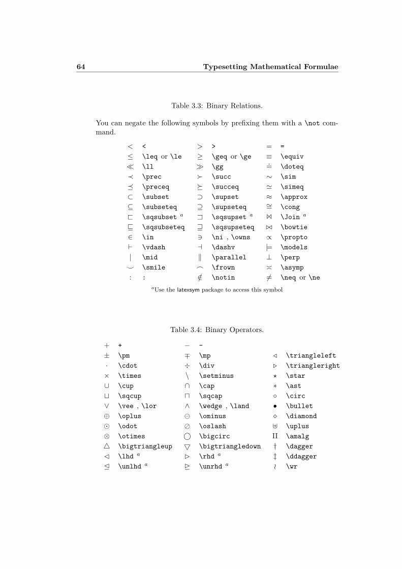
64 Typesetting Mathematical Formulae

Table 3.3: Binary Relations.

You can negate the following symbols by prefixing them with a \not com-mand.

< < > > = =≤ \leq or \le ≥ \geq or \ge ≡ \equiv \ll \gg .= \doteq≺ \prec \succ ∼ \sim \preceq \succeq ' \simeq⊂ \subset ⊃ \supset ≈ \approx⊆ \subseteq ⊇ \supseteq ∼= \cong@ \sqsubset a A \sqsupset a 1 \Join a

v \sqsubseteq w \sqsupseteq ./ \bowtie∈ \in 3 \ni , \owns ∝ \propto` \vdash a \dashv |= \models| \mid ‖ \parallel ⊥ \perp^ \smile _ \frown \asymp: : /∈ \notin 6= \neq or \ne

aUse the latexsym package to access this symbol

Table 3.4: Binary Operators.

+ + − -± \pm ∓ \mp / \triangleleft· \cdot ÷ \div . \triangleright× \times \ \setminus ? \star∪ \cup ∩ \cap ∗ \astt \sqcup u \sqcap \circ∨ \vee , \lor ∧ \wedge , \land • \bullet⊕ \oplus \ominus \diamond \odot \oslash ] \uplus⊗ \otimes © \bigcirc q \amalg4 \bigtriangleup 5 \bigtriangledown † \dagger \lhd a \rhd a ‡ \ddagger \unlhd a \unrhd a o \wr

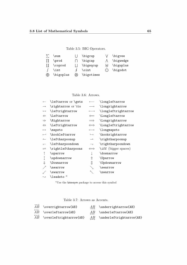
3.8 List of Mathematical Symbols 65

Table 3.5: BIG Operators.∑\sum

⋃\bigcup

∨\bigvee∏

\prod⋂

\bigcap∧

\bigwedge∐\coprod

⊔\bigsqcup

⊎\biguplus∫

\int∮

\oint⊙

\bigodot⊕\bigoplus

⊗\bigotimes

Table 3.6: Arrows.

← \leftarrow or \gets ←− \longleftarrow→ \rightarrow or \to −→ \longrightarrow↔ \leftrightarrow ←→ \longleftrightarrow⇐ \Leftarrow ⇐= \Longleftarrow⇒ \Rightarrow =⇒ \Longrightarrow⇔ \Leftrightarrow ⇐⇒ \Longleftrightarrow7→ \mapsto 7−→ \longmapsto← \hookleftarrow → \hookrightarrow \leftharpoonup \rightharpoonup \leftharpoondown \rightharpoondown \rightleftharpoons ⇐⇒ \iff (bigger spaces)↑ \uparrow ↓ \downarrowl \updownarrow ⇑ \Uparrow⇓ \Downarrow m \Updownarrow \nearrow \searrow \swarrow \nwarrow; \leadsto a

aUse the latexsym package to access this symbol

Table 3.7: Arrows as Accents.−−→AB \overrightarrowAB AB−−→ \underrightarrowAB←−−AB \overleftarrowAB AB←−− \underleftarrowAB←→AB \overleftrightarrowAB AB←→ \underleftrightarrowAB

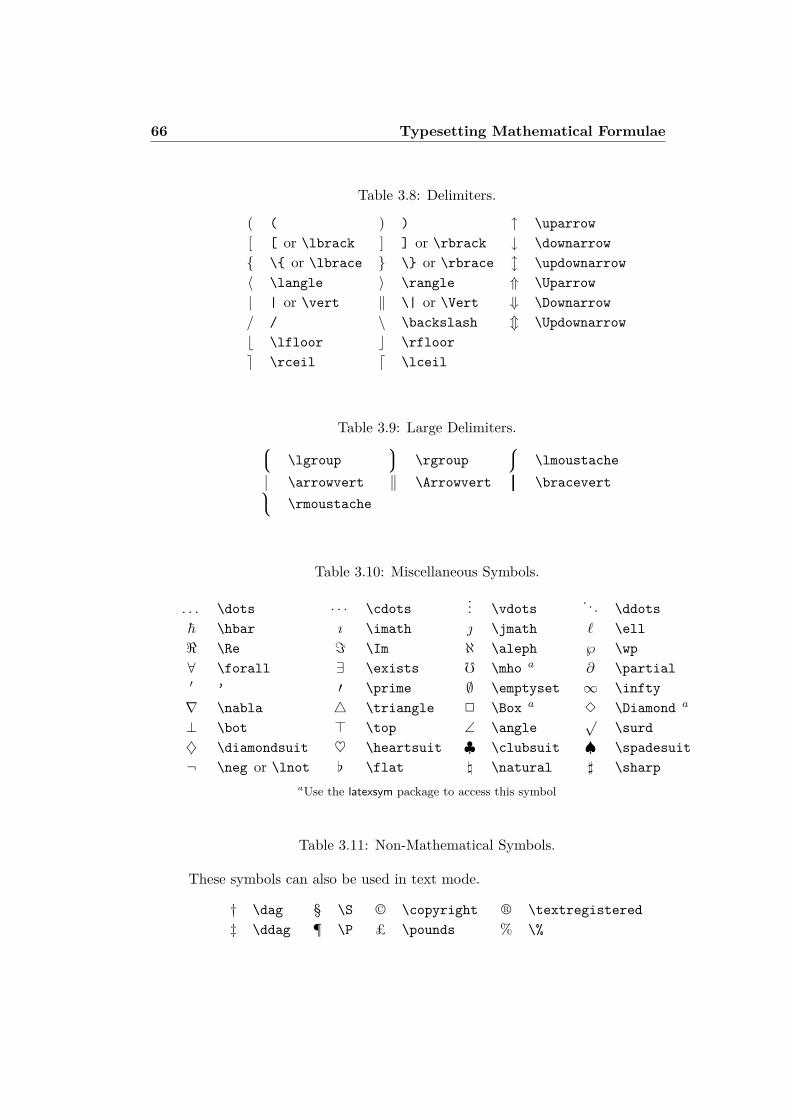
66 Typesetting Mathematical Formulae

Table 3.8: Delimiters.

( ( ) ) ↑ \uparrow[ [ or \lbrack ] ] or \rbrack ↓ \downarrow \ or \lbrace \ or \rbrace l \updownarrow〈 \langle 〉 \rangle ⇑ \Uparrow| | or \vert ‖ \| or \Vert ⇓ \Downarrow/ / \ \backslash m \Updownarrowb \lfloor c \rfloore \rceil d \lceil

Table 3.9: Large Delimiters. \lgroup \rgroup

\lmoustache \arrowvertww \Arrowvert

\bracevert \rmoustache

Table 3.10: Miscellaneous Symbols.

. . . \dots · · · \cdots... \vdots

. . . \ddots~ \hbar ı \imath \jmath ` \ell< \Re = \Im ℵ \aleph ℘ \wp∀ \forall ∃ \exists f \mho a ∂ \partial′ ’ ′ \prime ∅ \emptyset ∞ \infty∇ \nabla 4 \triangle 2 \Box a 3 \Diamond a

⊥ \bot > \top ∠ \angle√

\surd♦ \diamondsuit ♥ \heartsuit ♣ \clubsuit ♠ \spadesuit¬ \neg or \lnot [ \flat \ \natural ] \sharp

aUse the latexsym package to access this symbol

Table 3.11: Non-Mathematical Symbols.

These symbols can also be used in text mode.

† \dag § \S © \copyright ® \textregistered‡ \ddag ¶ \P £ \pounds % \%

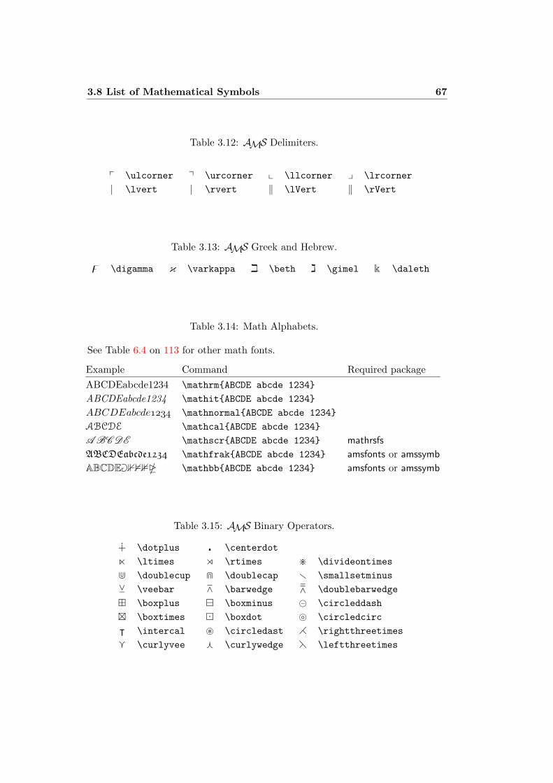
3.8 List of Mathematical Symbols 67

Table 3.12: AMS Delimiters.

p \ulcorner q \urcorner x \llcorner y \lrcorner| \lvert | \rvert ‖ \lVert ‖ \rVert

Table 3.13: AMS Greek and Hebrew.

z \digamma κ \varkappa i \beth ג \gimel k \daleth

Table 3.14: Math Alphabets.

See Table 6.4 on 113 for other math fonts.

Example Command Required packageABCDEabcde1234 \mathrmABCDE abcde 1234ABCDEabcde1234 \mathitABCDE abcde 1234ABCDEabcde1234 \mathnormalABCDE abcde 1234ABCDE \mathcalABCDE abcde 1234A BC DE \mathscrABCDE abcde 1234 mathrsfsABCDEabcde1234 \mathfrakABCDE abcde 1234 amsfonts or amssymbABCDEa1234 \mathbbABCDE abcde 1234 amsfonts or amssymb

Table 3.15: AMS Binary Operators.

u \dotplus \centerdotn \ltimes o \rtimes > \divideontimesd \doublecup e \doublecap r \smallsetminusY \veebar Z \barwedge [ \doublebarwedge \boxplus \boxminus \circleddash \boxtimes \boxdot \circledcircᵀ \intercal ~ \circledast i \rightthreetimesg \curlyvee f \curlywedge h \leftthreetimes

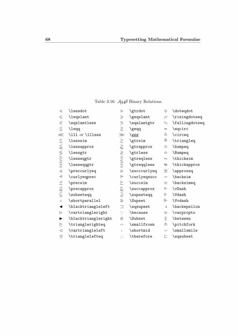
68 Typesetting Mathematical Formulae

Table 3.16: AMS Binary Relations.

l \lessdot m \gtrdot + \doteqdot6 \leqslant > \geqslant : \risingdotseq0 \eqslantless 1 \eqslantgtr ; \fallingdotseq5 \leqq = \geqq P \eqcirc≪ \lll or \llless ≫ \ggg $ \circeq. \lesssim & \gtrsim , \triangleq/ \lessapprox ' \gtrapprox l \bumpeq≶ \lessgtr ≷ \gtrless m \BumpeqQ \lesseqgtr R \gtreqless ∼ \thicksimS \lesseqqgtr T \gtreqqless ≈ \thickapprox4 \preccurlyeq < \succcurlyeq u \approxeq2 \curlyeqprec 3 \curlyeqsucc v \backsim- \precsim % \succsim w \backsimeqw \precapprox v \succapprox \vDashj \subseteqq k \supseteqq \Vdashq \shortparallel c \Supset \VvdashJ \blacktriangleleft A \sqsupset \backepsilonB \vartriangleright ∵ \because ∝ \varproptoI \blacktriangleright b \Subset G \betweenD \trianglerighteq a \smallfrown t \pitchforkC \vartriangleleft p \shortmid ` \smallsmileE \trianglelefteq ∴ \therefore @ \sqsubset

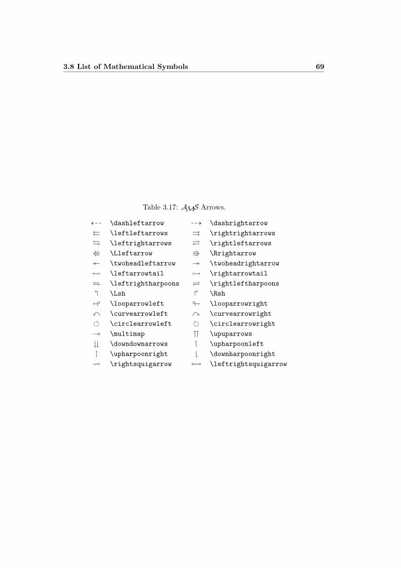
3.8 List of Mathematical Symbols 69

Table 3.17: AMS Arrows.

L99 \dashleftarrow 99K \dashrightarrow⇔ \leftleftarrows ⇒ \rightrightarrows \leftrightarrows \rightleftarrowsW \Lleftarrow V \Rrightarrow \twoheadleftarrow \twoheadrightarrow \leftarrowtail \rightarrowtail \leftrightharpoons \rightleftharpoons \Lsh \Rsh" \looparrowleft # \looparrowrightx \curvearrowleft y \curvearrowright \circlearrowleft \circlearrowright( \multimap \upuparrows \downdownarrows \upharpoonleft \upharpoonright \downharpoonright \rightsquigarrow ! \leftrightsquigarrow

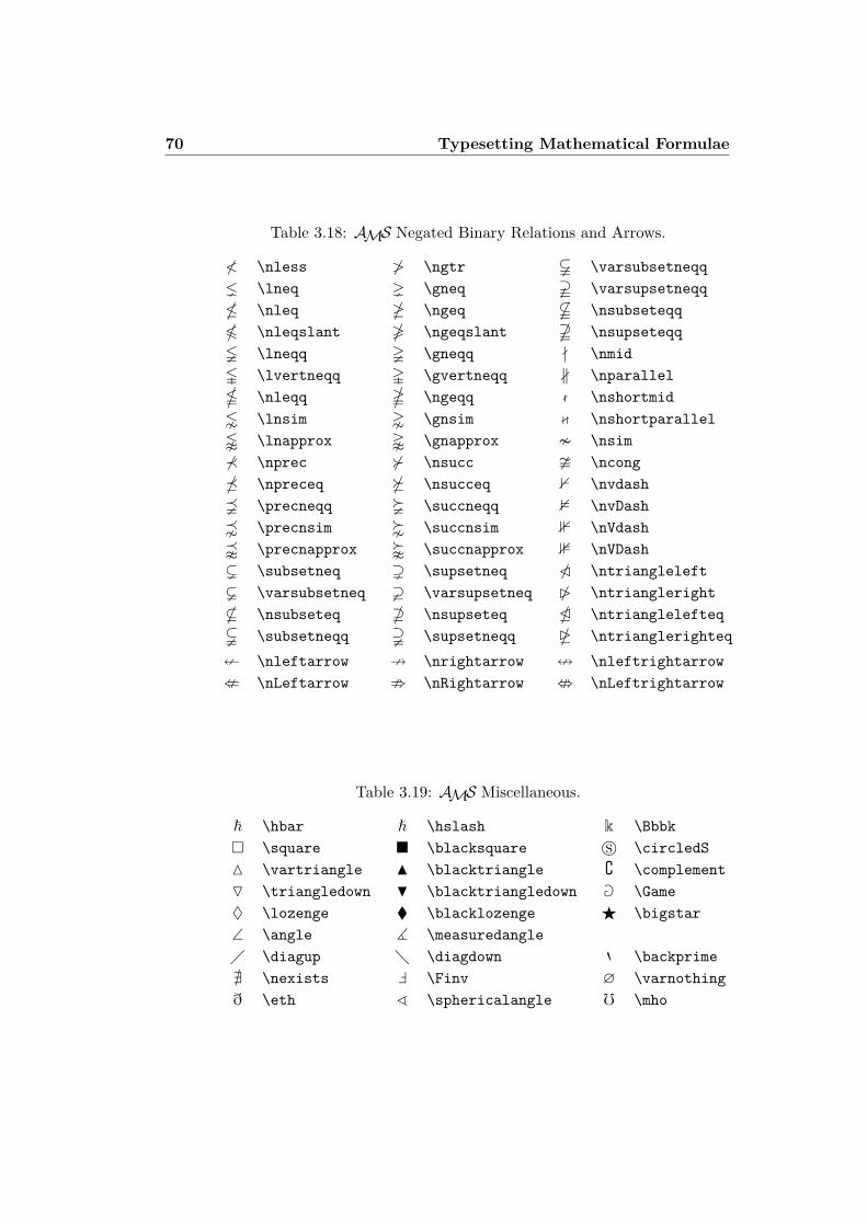
70 Typesetting Mathematical Formulae

Table 3.18: AMS Negated Binary Relations and Arrows.

≮ \nless ≯ \ngtr & \varsubsetneqq \lneq \gneq ' \varsupsetneqq \nleq \ngeq " \nsubseteqq \nleqslant \ngeqslant # \nsupseteqq \lneqq \gneqq - \nmid \lvertneqq \gvertneqq ∦ \nparallel \nleqq \ngeqq . \nshortmid \lnsim \gnsim / \nshortparallel \lnapprox \gnapprox \nsim⊀ \nprec \nsucc \ncong \npreceq \nsucceq 0 \nvdash \precneqq \succneqq 2 \nvDash \precnsim \succnsim 1 \nVdash \precnapprox \succnapprox 3 \nVDash( \subsetneq ) \supsetneq 6 \ntriangleleft \varsubsetneq ! \varsupsetneq 7 \ntriangleright* \nsubseteq + \nsupseteq 5 \ntrianglelefteq$ \subsetneqq % \supsetneqq 4 \ntrianglerighteq

8 \nleftarrow 9 \nrightarrow = \nleftrightarrow: \nLeftarrow ; \nRightarrow < \nLeftrightarrow

Table 3.19: AMS Miscellaneous.

~ \hbar \hslash k \Bbbk \square \blacksquare s \circledSM \vartriangle N \blacktriangle \complementO \triangledown H \blacktriangledown a \Game♦ \lozenge \blacklozenge F \bigstar∠ \angle ] \measuredangle \diagup \diagdown 8 \backprime@ \nexists ` \Finv ∅ \varnothingð \eth ^ \sphericalangle f \mho

Chapter 4

Specialities

When putting together a large document, LATEX will help you with some specialfeatures like index generation, bibliography management, and other things. Amuch more complete description of specialities and enhancements possible withLATEX can be found in the LATEX Manual [1] and The LATEX Companion [3].

4.1 Including Encapsulated PostScriptLATEX provides the basic facilities to work with floating bodies, such asimages or graphics, with the figure and table environments.

There are several ways to generate the actual graphics with basic LATEXor a LATEX extension package, a few of them are described in chapter 5.Please refer to The LATEX Companion [3] and the LATEX Manual [1] formore information on that subject.

A much easier way to get graphics into a document is to generate themwith a specialised software package1 and then include the finished graphicsinto the document. Here again, LATEX packages offer many ways to do this,but this introduction will only discuss the use of Encapsulated PostScript(EPS) graphics, because it is quite easy to do and widely used. In orderto use pictures in the EPS format, you must have a PostScript printer2

available for output.A good set of commands for inclusion of graphics is provided in the

graphicx package by D. P. Carlisle. It is part of a whole family of packagescalled the “graphics” bundle.3

Assuming you are working on a system with a PostScript printer avail-able for output and with the graphicx package installed, you can use thefollowing step by step guide to include a picture into your document:

1Such as XFig, CorelDraw!, Freehand, Gnuplot, . . .2Another possibility to output PostScript is the GhostScript program available

from support/ghostscript. Windows and OS/2 users might want to look for GSview.3macros/latex/required/graphics

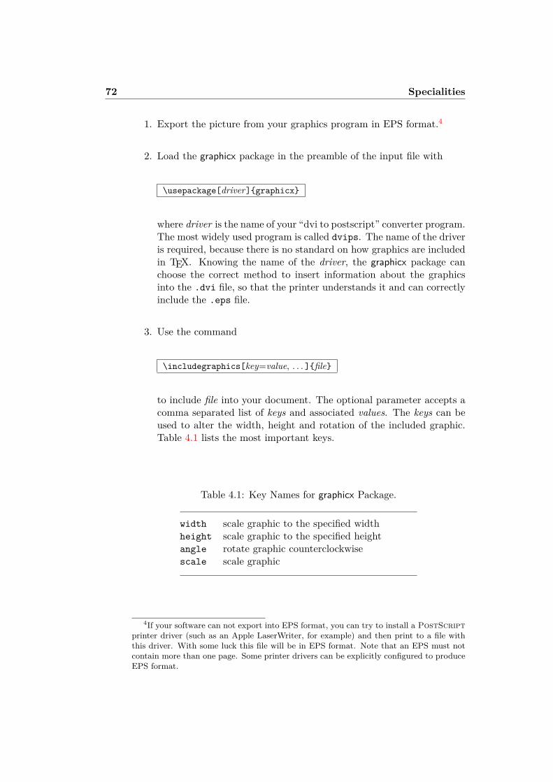
72 Specialities

1. Export the picture from your graphics program in EPS format.4

2. Load the graphicx package in the preamble of the input file with

\usepackage[driver]graphicx

where driver is the name of your “dvi to postscript” converter program.The most widely used program is called dvips. The name of the driveris required, because there is no standard on how graphics are includedin TEX. Knowing the name of the driver, the graphicx package canchoose the correct method to insert information about the graphicsinto the .dvi file, so that the printer understands it and can correctlyinclude the .eps file.

3. Use the command

\includegraphics[key=value, . . . ]file

to include file into your document. The optional parameter accepts acomma separated list of keys and associated values. The keys can beused to alter the width, height and rotation of the included graphic.Table 4.1 lists the most important keys.

Table 4.1: Key Names for graphicx Package.

width scale graphic to the specified widthheight scale graphic to the specified heightangle rotate graphic counterclockwisescale scale graphic

4If your software can not export into EPS format, you can try to install a PostScriptprinter driver (such as an Apple LaserWriter, for example) and then print to a file withthis driver. With some luck this file will be in EPS format. Note that an EPS must notcontain more than one page. Some printer drivers can be explicitly configured to produceEPS format.

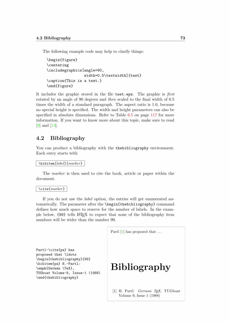
4.2 Bibliography 73

The following example code may help to clarify things:

\beginfigure\centering\includegraphics[angle=90,

width=0.5\textwidth]test\captionThis is a test.\endfigure

It includes the graphic stored in the file test.eps. The graphic is firstrotated by an angle of 90 degrees and then scaled to the final width of 0.5times the width of a standard paragraph. The aspect ratio is 1.0, becauseno special height is specified. The width and height parameters can also bespecified in absolute dimensions. Refer to Table 6.5 on page 117 for moreinformation. If you want to know more about this topic, make sure to read[9] and [13].

4.2 BibliographyYou can produce a bibliography with the thebibliography environment.Each entry starts with

\bibitem[label]marker

The marker is then used to cite the book, article or paper within thedocument.

\citemarker

If you do not use the label option, the entries will get enumerated au-tomatically. The parameter after the \beginthebibliography commanddefines how much space to reserve for the number of labels. In the exam-ple below, 99 tells LATEX to expect that none of the bibliography itemnumbers will be wider than the number 99.

Partl~\citepa hasproposed that \ldots\beginthebibliography99\bibitempa H.~Partl:\emphGerman \TeX,TUGboat Volume~9, Issue~1 (1988)\endthebibliography

Partl [1] has proposed that . . .

Bibliography

[1] H. Partl: German TEX, TUGboatVolume 9, Issue 1 (1988)

74 Specialities

For larger projects, you might want to check out the BibTEX program.BibTEX is included with most TEX distributions. It allows you to main-tain a bibliographic database and then extract the references relevant tothings you cited in your paper. The visual presentation of BibTEX gener-ated bibliographies is based on a style sheets concept that allows you tocreate bibliographies following a wide range of established designs.

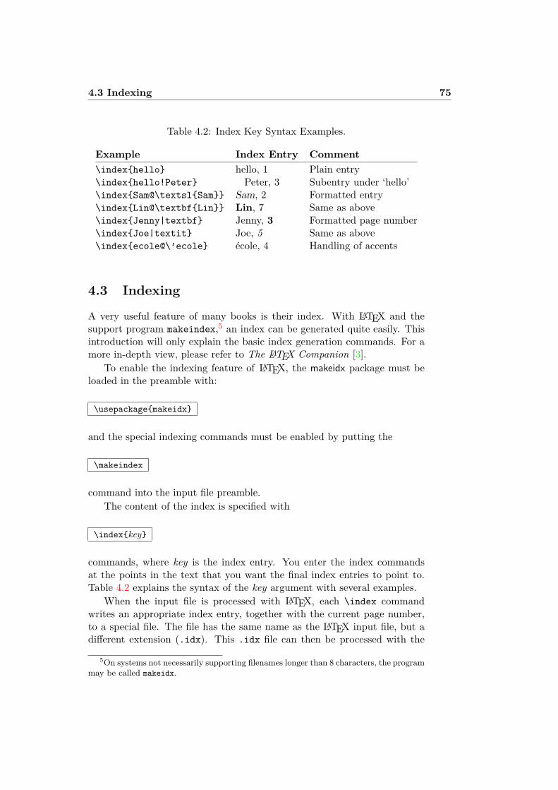
4.3 Indexing 75

Table 4.2: Index Key Syntax Examples.

Example Index Entry Comment\indexhello hello, 1 Plain entry\indexhello!Peter Peter, 3 Subentry under ‘hello’\indexSam@\textslSam Sam, 2 Formatted entry\indexLin@\textbfLin Lin, 7 Same as above\indexJenny|textbf Jenny, 3 Formatted page number\indexJoe|textit Joe, 5 Same as above\indexecole@\’ecole école, 4 Handling of accents

4.3 Indexing

A very useful feature of many books is their index. With LATEX and thesupport program makeindex,5 an index can be generated quite easily. Thisintroduction will only explain the basic index generation commands. For amore in-depth view, please refer to The LATEX Companion [3].

To enable the indexing feature of LATEX, the makeidx package must beloaded in the preamble with:

\usepackagemakeidx

and the special indexing commands must be enabled by putting the

\makeindex

command into the input file preamble.The content of the index is specified with

\indexkey

commands, where key is the index entry. You enter the index commandsat the points in the text that you want the final index entries to point to.Table 4.2 explains the syntax of the key argument with several examples.

When the input file is processed with LATEX, each \index commandwrites an appropriate index entry, together with the current page number,to a special file. The file has the same name as the LATEX input file, but adifferent extension (.idx). This .idx file can then be processed with the

5On systems not necessarily supporting filenames longer than 8 characters, the programmay be called makeidx.

76 Specialities

makeindex program.

makeindex filename

The makeindex program generates a sorted index with the same basefile name, but this time with the extension .ind. If now the LATEX inputfile is processed again, this sorted index gets included into the document atthe point where LATEX finds

\printindex

The showidx package that comes with LATEX2ε prints out all index en-tries in the left margin of the text. This is quite useful for proofreading adocument and verifying the index.

Note that the \index command can affect your layout if not used care-fully.

My Word \indexWord. As opposedto Word\indexWord. Note theposition of the full stop.

My Word . As opposed to Word. Notethe position of the full stop.

4.4 Fancy Headers

The fancyhdr package,6 written by Piet van Oostrum, provides a few sim-ple commands that allow you to customize the header and footer lines ofyour document. If you look at the top of this page, you can see a possibleapplication of this package.

The tricky problem when customising headers and footers is to get thingslike running section and chapter names in there. LATEX accomplishes thiswith a two-stage approach. In the header and footer definition, you usethe commands \rightmark and \leftmark to represent the current sectionand chapter heading, respectively. The values of these two commands areoverwritten whenever a chapter or section command is processed.

For ultimate flexibility, the \chapter command and its friends do notredefine \rightmark and \leftmark themselves. They call yet another com-mand (\chaptermark, \sectionmark, or \subsectionmark) that is respon-sible for redefining \rightmark and \leftmark.

If you want to change the look of the chapter name in the header line,you need only “renew” the \chaptermark command.

6Available from macros/latex/contrib/supported/fancyhdr.

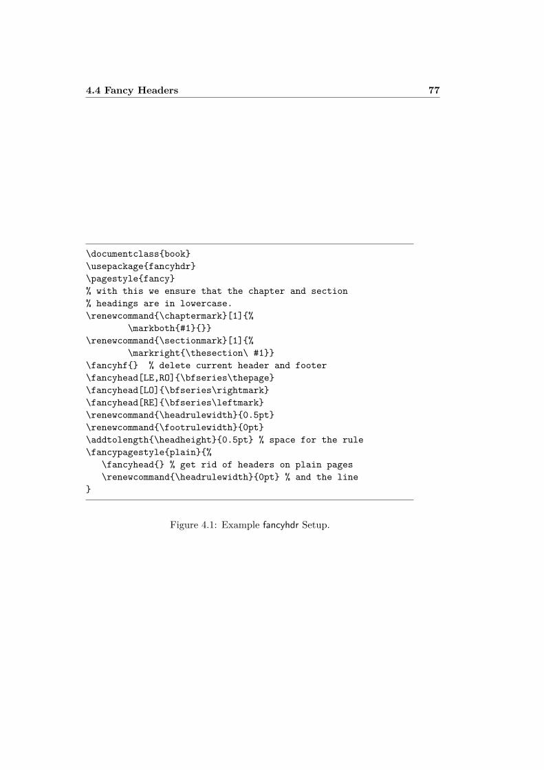
4.4 Fancy Headers 77

\documentclassbook\usepackagefancyhdr\pagestylefancy% with this we ensure that the chapter and section% headings are in lowercase.\renewcommand\chaptermark[1]%

\markboth#1\renewcommand\sectionmark[1]%

\markright\thesection\ #1\fancyhf % delete current header and footer\fancyhead[LE,RO]\bfseries\thepage\fancyhead[LO]\bfseries\rightmark\fancyhead[RE]\bfseries\leftmark\renewcommand\headrulewidth0.5pt\renewcommand\footrulewidth0pt\addtolength\headheight0.5pt % space for the rule\fancypagestyleplain%

\fancyhead % get rid of headers on plain pages\renewcommand\headrulewidth0pt % and the line

Figure 4.1: Example fancyhdr Setup.

78 Specialities

Figure 4.1 shows a possible setup for the fancyhdr package that makes theheaders look about the same as they look in this booklet. In any case, I sug-gest you fetch the documentation for the package at the address mentionedin the footnote.

4.5 The Verbatim Package

Earlier in this book, you got to know the verbatim environment. In thissection, you are going to learn about the verbatim package. The verbatimpackage is basically a re-implementation of the verbatim environment thatworks around some of the limitations of the original verbatim environment.This by itself is not spectacular, but the implementation of the verbatimpackage added new functionality, which is why I am mentioning the packagehere. The verbatim package provides the

\verbatiminputfilename

command, which allows you to include raw ASCII text into your documentas if it were inside a verbatim environment.

As the verbatim package is part of the ‘tools’ bundle, you should find itpre-installed on most systems. If you want to know more about this package,make sure to read [10].

4.6 Installing Extra Packages

Most LATEX installations come with a large set of pre-installed style packages,but many more are available on the net. The main place to look for stylepackages on the Internet is CTAN (http://www.ctan.org/).

Packages such as geometry, hyphenat, and many others are typicallymade up of two files: a file with the extension .ins and another with theextension .dtx. There will often be a readme.txt with a brief descriptionof the package. You should of course read this file first.

In any event, once you have copied the package files onto your machine,you still have to process them in a way that (a) tells your TEX distributionabout the new style package and (b) gives you the documentation. Here’show you do the first part:

1. Run LATEX on the .ins file. This will extract a .sty file.

2. Move the .sty file to a place where your distribution can find it. Usu-ally this is in your .../localtexmf/tex/latex subdirectory (Win-dows or OS/2 users should feel free to change the direction of theslashes).

4.7 Working with pdfLATEX 79

3. Refresh your distribution’s file-name database. The command dependson the LATEXdistribution you use: teTeX, fpTeX – texhash; web2c –maktexlsr; MikTeX – initexmf -update-fndb or use the GUI.

Now you can extract the documentation from the .dtx file:

1. Run LATEX on the .dtx file. This will generate a .dvi file. Notethat you may have to run LATEX several times before it gets the cross-references right.

2. Check to see if LATEX has produced a .idx file among the various filesyou now have. If you do not see this file, then you may proceed tostep 5.

3. In order to generate the index, type the following:makeindex -s gind.ist name(where name stands for the main-file name without any extension).

4. Run LATEX on the .dtx file once again.

5. Last but not least, make a .ps or .pdf file to increase your readingpleasure.

Sometimes you will see that a .glo (glossary) file has been produced.Run the following command between step 4 and 5:makeindex -s gglo.ist -o name.gls name.gloBe sure to run LATEX on the .dtx one last time before moving on to step 5.

4.7 Working with pdfLATEXBy Daniel Flipo <Daniel.Flipo@univ-lille1.fr>

PDF is a hypertext document format. Much like in a web page, some wordsin the document are marked as hyperlinks. They link to other places in thedocument or even to other documents. If you click on such a hyperlink youget transported to the destination of the link. In the context of LATEX, thismeans that all occurrences of \ref and \pageref become hyperlinks. Addi-tionally, the table of contents, the index and all the other similar structuresbecome collections of hyperlinks.

Most web pages you find today are written in HTML (HyperText MarkupLanguage). This format has two significant disadvantages when writingscientific documents:

1. Including mathematical formulae into HTML documents is not gener-ally supported. While there is a standard for it, most browsers usedtoday do not support it, or lack the required fonts.

80 Specialities

2. Printing HTML documents is possible, but the results vary widelybetween platforms and browsers. The results are miles removed fromthe quality we have come to expect in the LATEX world.

There have been many attempts to create translators from LATEX toHTML. Some were even quite successful in the sense that they are ableto produce legible web pages from a standard LATEX input file. But all ofthem cut corners left and right to get the job done. As soon as you startusing more complex LATEX features and external packages things tend tofall apart. Authors wishing to preserve the unique typographic quality oftheir documents even when publishing on the web turn to PDF (PortableDocument Format), which preserves the layout of the document and permitshypertext navigation. Most modern browsers come with plugins that allowthe direct display of PDF documents.

Even though there are DVI and PS viewers for almost every platform,you will find that Acrobat Reader and Xpdf for viewing PDF documents aremore widely deployed. So providing PDF versions of your documents willmake them much more accessible to your potential readers.

4.7.1 PDF Documents for the Web

The creation of a PDF file from LATEX source is very simple, thanks to thepdfTEX program developed by Hàn Thê Thành. pdfTEX produces PDFoutput where normal TEX produces DVI. There is also a pdfLATEX, whichproduces PDF output from LATEX sources.

Both pdfTEX and pdfLATEX are installed automatically by most modernTEX distributions, such as teTEX, fpTEX, MikTEX, TEXLive and CMacTEX.

To produce a PDF instead of DVI, it is sufficient to replace the com-mand latex file.tex by pdflatex file.tex. On systems where LATEXis not called from the command line, you may find a special button in theTEXControlCenter.

In LATEX you can define the paper size with an optional documentclassargument such as a4paper or letterpaper. This works in pdfLATEX too,but on top of this pdfTEX also needs to know the physical size of the paperto determine the physical size of the pages in the pdf file. If you use thehyperref package (see page 83), the papersize will be adjusted automatically.Otherwise you have to do this manually by putting the following lines intothe preamble of the document:

\pdfpagewidth=\paperwidth\pdfpageheight=\paperheight

The following section will go into more detail regarding the differencesbetween normal LATEX and pdfLATEX. The main differences concern threeareas: the fonts to use, the format of images to include, and the manualconfiguration of hyperlinks.

4.7 Working with pdfLATEX 81

4.7.2 The Fonts

pdfLATEX can deal with all sorts of fonts (PK bitmaps, TrueType, PostScripttype 1. . . ) but the normal LATEX font format, the bitmap PK fonts producevery ugly results when the document is displayed with Acrobat Reader. Itis best to use PostScript Type 1 fonts exclusively to produce documentsthat display well. Modern TeX installations will be setup so that this hap-pens automatically. Best is to try. If it works for you, just skip this wholesection.

The PostScript Type 1 implementation of the Computer Modern andAMSFonts was produced by Blue Sky Research and Y&Y, Inc., who thentransferred copyright to the American Mathematical Society. The fonts weremade publicly available in early 1997 and currently come with most of TEXdistributions.

However, if you are using LATEX to create documents in languages otherthan English, you might want to use EC, LH, or CB fonts (see the discussionabout OT1 fonts on the page 26). Vladimir Volovich has created the cm-superfont bundle which covers the entire EC/TC, EC Concrete, EC Bright andLH font sets. It is available from CTAN:/fonts/ps-type1/cm-super and isincluded with TEXLive7 and MikTEX. Similar type 1 CB Greek fonts createdby Apostolos Syropoulos are available at CTAN:/tex-archive/fonts/greek/cb.Unfortunately, both of these font sets are not of the same typographic qual-ity as the Type1 CM fonts by Blue Sky/Y&Y. They were automaticallyhinted, and the document might look not as neat on the screen as the onesusing Blue Sky/Y&Y type 1 CM fonts, on high resolution output devicesthey produce results identical to the original bitmap EC/LH/CB fonts.

If you are creating document in one of Latin-based languages, you haveseveral other options.

• You might want to use aeguill package, aka Almost European ComputerModern with Guillemets. Just put the line\usepackageaeguill into the preamble of your document, to enableAE virtual fonts instead of EC fonts.

• Alternatively, you can use mltex package, but this only works whenyour pdfTEX has been compiled with the mltex option.

The AE virtual fontset, like the MlTEX system, makes TEX believe it hasa full 256 character fontset at its disposal by creating most of the missingletters from characters of the CM font and rearranging them in the EC order,this allows to use the excellent type 1 format CM fonts available on mostsystems. As the font is now in T1 encoding, hyphenation will work well inLatin-based European languages. The only disadvantage of this approach isthat the artificial AE characters do not work with Acrobat Reader’s Findfunction, so you cannot search for words with accented characters in yourfinal PDF file.

82 Specialities

For the Russian language a similar solution is to use C1 virtual fontsavailable at ftp://ftp.vsu.ru/pub/tex/font-packs/c1fonts. These fontscombine the standard CM type 1 fonts from Bluesky collection and CMCYRtype 1 fonts from Paradissa and BaKoMa collection, all available on CTAN.Because Paradissa fonts contain only Russian letters, C1 fonts are missingother Cyrillic glyphs.

Another solution is to switch to other PostScript type 1 fonts. Ac-tually, some of them are even included with every copy of Acrobat Reader.Because these fonts have different character sizes, the text layout on yourpages will change. Generally these other fonts will use more space than theCM fonts, which are very space-efficient. Also, the overall visual coherenceof your document will suffer because Times, Helvetica and Courier (the pri-mary candidates for such a replacement job) have not been designed to workin harmony in a single document.

Two ready-made font sets are available for this purpose: pxfonts, whichis based on Palatino as its main text body font, and the txfonts package,which is based on Times. To use them it is sufficient to put the followinglines into the preamble of your document:

\usepackage[T1]fontenc\usepackagepxfonts

Note: you may find lines like

Warning: pdftex (file eurmo10): Font eur... not found

in the .log file after compiling your input file. They mean that some fontused in the document has not been found. You really have to fix theseproblems, as the resulting PDF document may not display the pages withthe missing characters at all.

As you can see this whole font business, especially the lack of a goodEC fontset equivalent in quality to the CM font in type 1 format, has beenoccupying many peoples minds. Recently a new set of high quality outlinefonts called Latin Modern (LM) has become available. It puts an end to themisery. If you have a recent TEX installation, chances are that you alreadyhave a copy of them installed all you need todo is to add

\usepackagelmodern\usepackage[T1]fontenc\usepackagetextcomp

to the preamble of your document and you are all set for creating excellentpdf output with full support for the full Latin character set.

4.7 Working with pdfLATEX 83

4.7.3 Using Graphics

Including graphics into a document works best with the graphicx package(see page 71). By using the special driver option pdftex the package willwork with pdfLATEX as well:

\usepackage[pdftex]color,graphicx

In the sample above I have included the color option, as using color indocuments displayed on the web comes quite naturally.

So much for the good news. The bad news is that graphics in Encapsu-lated PostScript format do not work with PdfLATEX. If you don’t define afile extension in the \includegraphics command, graphicx will go lookingfor a suitable file on its own, depending on the setting of the driver option.For pdftex this is formats .png, .pdf, .jpg and .mps ( METAPOST)—butnot .eps.

The simple way out of this problem is to just convert your EPS files intoPDF format using the epstopdf utility found on many systems. For vectorgraphics (drawings) this is a great solution. For bitmaps (photos, scans)this is not ideal, because the PDF format natively supports the inclusionof PNG and JPEG images. PNG is good for screenshots and other imageswith few colors. JPEG is great for photos, as it is very space-efficient.

It may even be desirable not to draw certain geometric figures, but ratherdescribe the figure with a specialized command language, such as META-POST, which can be found in most TEX distributions, and comes with itsown extensive manual.

4.7.4 Hypertext Links

The hyperref package will take care of turning all internal references of yourdocument into hyperlinks. For this to work properly some magic is necessary,so you have to put \usepackage[pdftex]hyperref as the last commandinto the preamble of your document.

Many options are available to customize the behaviour of the hyperrefpackage:

• either as a comma separated list after the pdftex option\usepackage[pdftex]hyperref

• or on individual lines with the command \hypersetupoptions.The only required option is pdftex; the others are optional and allow

you to change the default behaviour of hyperref.7 In the following list thedefault values are written in an upright font.

7It is worth noting that the hyperref package is not limited to work with pdfTEX. Itcan also be configured to embed PDF-specific information into the DVI output of normalLATEX, which then gets put into the PS file by dvips and is finally picked up by AdobeDistiller when it is used to turn the PS file into PDF.

84 Specialities

bookmarks (=true,false) show or hide the bookmarks bar whendisplaying the document

unicode (=false,true) allows to use characters of non-latin basedlanguages in Acrobat’s bookmarks

pdftoolbar (=true,false) show or hide Acrobat’s toolbar

pdfmenubar (=true,false) show or hide Acrobat’s menu

pdffitwindow (=true,false) adjust the initial magnification of the pdfwhen displayed

pdftitle (=text) define the title that gets displayed in the DocumentInfo window of Acrobat

pdfauthor (=text) the name of the PDF’s author

pdfnewwindow (=true,false) define if a new window should get openedwhen a link leads out of the current document

colorlinks (=false,true) surround the links by color frames (false)or colors the text of the links (true). The color of these links can beconfigured using the following options (default colors are shown):

linkcolor (=red) color of internal links (sections, pages, etc.),citecolor (=green) color of citation links (bibliography)filecolor (=magenta) color of file linksurlcolor (=cyan) color of URL links (mail, web)

If you are happy with the defaults, use

\usepackage[pdftex]hyperref

To have the bookmark list open and links in color (the =true values areoptional):

\usepackage[pdftex,bookmarks,colorlinks]hyperref

When creating PDFs destined for printing, colored links are not a goodthing as they end up in gray in the final output, making it difficult to read.You can use color frames, which are not printed:

\usepackagehyperref\hypersetupcolorlinks=false

or make links black:

4.7 Working with pdfLATEX 85

\usepackagehyperref\hypersetupcolorlinks,%

citecolor=black,%filecolor=black,%linkcolor=black,%urlcolor=black,%pdftex

When you just want to provide information for the Document Info sec-tion of the PDF file:

\usepackage[pdfauthor=Pierre Desproges,%pdftitle=Des femmes qui tombent,%pdftex]hyperref

In addition to the automatic hyperlinks for cross references, it is possibleto embed explicit links using

\hrefurltext

The code

The \hrefhttp://www.ctan.orgCTAN website.

produces the output “CTAN”; a click on the word “CTAN” will take you tothe CTAN website.

If the destination of the link is not a URL but a local file, you can usethe \href command:

The complete document is \hrefmanual.pdfhere

Which produces the text “The complete document is here”. A click on theword “here” will open the file manual.pdf. (The filename is relative to thelocation of the current document).

The author of an article might want her readers to easily send emailmessages by using the \href command inside the \author command on thetitle page of the document:

\authorMary Oetiker $<$\hrefmailto:mary@oetiker.ch%mary@oetiker.ch$>$

Note that I have put the link so that my email address appears not only inthe link but also on the page itself. I did this because the link\hrefmailto:mary@oetiker.chMary Oetikerwould work well within Acrobat, but once the page is printed the emailaddress would not be visible anymore.

86 Specialities

4.7.5 Problems with Links

Messages like the following:

! pdfTeX warning (ext4): destination with the sameidentifier (namepage.1) has been already used,duplicate ignored

appear when a counter gets reinitialized, for example by using the command\mainmatter provided by the book document class. It resets the page num-ber counter to 1 prior to the first chapter of the book. But as the preface ofthe book also has a page number 1 all links to “page 1” would not be uniqueanymore, hence the notice that “duplicate has been ignored.”

The counter measure consists of putting plainpages=false into thehyperref options. This unfortunately only helps with the page counter. Aneven more radical solution is to use the optionhypertexnames=false, but this will cause the page links in the index tostop working.

4.7.6 Problems with Bookmarks

The text displayed by bookmarks does not always look like you expect itto look. Because bookmarks are “just text,” much fewer characters areavailable for bookmarks than for normal LATEX text. Hyperref will normallynotice such problems and put up a warning:

Package hyperref Warning:Token not allowed in a PDFDocEncoded string:

You can now work around this problem by providing a text string for thebookmarks, which replaces the offending text:

\texorpdfstringTEX textBookmark Text

Math expressions are a prime candidate for this kind of problem:

\section\texorpdfstring$E=mc^2$%E=mc^2

which turns \section$E=mc^2$ to “E=mc2” in the bookmark area.Color changes also do not travel well into bookmarks:

\section\textcolorredRed !

produces the string “redRed!”. The command \textcolor gets ignored butits argument (red) gets printed.

If you use

4.7 Working with pdfLATEX 87

\section\texorpdfstring\textcolorredRed !Red\ !

the result will be much more legible.If you write your document in unicode and use the unicode option for

the hyperref package you can use unicode characters in bookmarks. Thiswill give you a much larger selection of characters to pick from when whenusing \texorpdfstring.

Source Compatibility Between LATEX and pdfLATEX

Ideally your document would compile equally well with LATEX and pdfLATEX.The main problem in this respect is the inclusion of graphics. The simplesolution is to systematically drop the file extension from \includegraphicscommands. They will then automatically look for a file of a suitable formatin the current directory. All you have to do is create appropriate versions ofthe graphics files. LATEX will look for .eps, and pdfLATEX will try to includea file with the extension .png, .pdf, .jpg or .mps (in that order).

For the cases where you want to use different code for the PDF versionof your document, you can simply add the package ifpdf8 to your preamble.Chances are that you already have it installed; if not then you’re probablyusing MiKTEX which will install it for you automatically the first time youtry to use it. This package defines the special command \ifpdf that willallow you to write conditional code easily. In this example, we want thePostScript version to be black and white due to the printing costs but wewant the PDF version for online viewing to be colourful.

\RequirePackageifpdf % running on pdfTeX?\ifpdf\documentclass[a4paper,12pt,pdftex]book

\else\documentclass[a4paper,12pt,dvips]book

\fi

\ifpdf\usepackagelmodern

\fi\usepackage[bookmarks, % add hyperlinks

colorlinks,plainpages=false]hyperref

\usepackage[T1]fontenc\usepackage[latin1]inputenc\usepackage[english]babel

8If you want the whole story on why to use this package then go to the TEX FAQ underthe itemhttp://www.tex.ac.uk/cgi-bin/texfaq2html?label=ifpdf.

88 Specialities

\usepackagegraphicx...

In the example above I have included the hyperref package even in the non-PDF version. The effect of this is to make the \href command work in allcases, which saves me from wrapping every occurrence into a conditionalstatement.

Note that in recent TEX distributions (TEXLive for example), the nor-mal TEX program is actually pdfTEX it will automatically switch betweenproducing pdf and dvi according to the settings in the document class. Ifyou use the code above then you can still use the pdflatex command to getpdf output and latex for normal dvi output.

4.8 Creating PresentationsBy Daniel Flipo <Daniel.Flipo@univ-lille1.fr>

You can present the results of your scientific work on a blackboard, withtransparencies, or directly from your laptop using some presentation soft-ware.

pdfLATEX combined with the beamer class allows you to create presen-tations in PDF, looking much like something you might be able to generatewith PowerPoint if you had a very good day, but much more portable be-cause Acrobat Reader is available on many more systems.

The beamer class uses graphicx, color and hyperref with options adaptedto screen presentations.

When you compile the code presented in figure 4.2 with PDFLATEX youget a PDF file with a title page and a second page showing several itemsthat will be reveled one at a time as you step though your presentation.

One of the advantages of the beamer class is that it produces a PDF filethat is directly usable without first going through a PostScript stage likeprosper or requiring additional post processing like presentations createdwith the ppower4 package.

With the beamer class you can produce several versions (modes) of yourdocument from the same input file. The input file may contain specialinstructions for the different modes in angular brackets. The following modesare available.

beamer for the presentation PDF discussed above.

trans for slides.

handout for the printed version.

The default mode is beamer, you can change it by setting a different modeas a global option, like \documentclass[10pt,handout]beamer to printthe handouts for example.

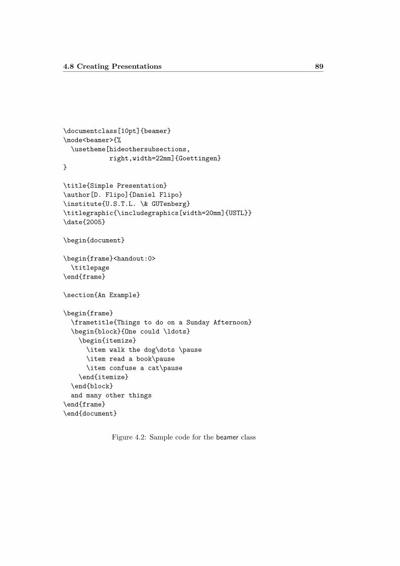
4.8 Creating Presentations 89

\documentclass[10pt]beamer\mode<beamer>%\usetheme[hideothersubsections,

right,width=22mm]Goettingen

\titleSimple Presentation\author[D. Flipo]Daniel Flipo\instituteU.S.T.L. \& GUTenberg\titlegraphic\includegraphics[width=20mm]USTL\date2005

\begindocument

\beginframe<handout:0>\titlepage

\endframe

\sectionAn Example

\beginframe\frametitleThings to do on a Sunday Afternoon\beginblockOne could \ldots

\beginitemize\item walk the dog\dots \pause\item read a book\pause\item confuse a cat\pause

\enditemize\endblockand many other things

\endframe\enddocument

Figure 4.2: Sample code for the beamer class

90 Specialities

The look of the screen presentation depends on the theme you choose.You can either pick one of the themes shipped with the beamer class oryou can even create your own. See the beamer class documentation inbeameruserguide.pdf for more information on this.

Lets have a closer look at the code in figure 4.2.For the screen version of the presentation \mode<beamer> we have chosen

the Goettingen theme to show a navigation panel integrated into the tableof contents. The options allow to choose the size of the panel (22 mm inthis case) and its position (on the right side of the body text). The optionhideothersubsections, shows the chapter titles, but only the subsections ofthe present chapter. There are no special settings for \mode<trans> and\mode<handout>. They appear in their standard layout.

The commands \title, \author, \institute, and\titlegraphic set the content of the title page. The optional argumentsof \title[] and \author[] let you specify a special version of the titleand the author name to be displayed on the panel of the Goettingen theme.

The titles and subtitles in the panel are created with normal \sectionand \subsection commands that you place outside the frame environ-ment.

The tiny navigation icons at the bottom of the screen also allow tonavigate the document. Their presence is not dependent on the theme youchoose.

The contents of each slide or screen has to be placed inside a frameenvironment. There is an optional argument in angular brackets (< and>), it allows to suppress a particular frame in one of the versions of thepresentation. In the example the first page would not be shown in thehandout version due to the <handout:0> argument.

It is highly recommended to set a title for each slide apart from thetitle slide. This is done with the command \frametitle. If a subtitleis necessary you can use the block environment as shown in the example.Note that the sectioning commands \section and \subsection do notproduce output on the slide proper.

The command \pause in the itemize environment lets you reveal theitems one by one. For other presentation effects check out the commands\only, \uncover, \alt and \temporal. In many place you can also useangular brakes to further customize the presentation.

In any case make sure you read through the beamer class documenta-tion beameruserguide.pdf to get a complete picture of what is in storefor you. This package is being actively developed, check out their websitehttp://latex-beamer.sourceforge.net/ to get the latest information.

Chapter 5

Producing MathematicalGraphics

Most people use LATEX for typesetting their text. But as the non content andstructure oriented approach to authoring is so convenient, LATEX also offers a, ifsomewhat restricted, possibility for producing graphical output from textual de-scriptions. Furthermore, quite a number of LATEX extensions have been createdin order to overcome these restrictions. In this section, you will learn about afew of them.

5.1 OverviewThe picture environment allows programming pictures directly in LATEX.A detailed description can be found in the LATEX Manual [1]. On the onehand, there are rather severe constraints, as the slopes of line segmentsas well as the radii of circles are restricted to a narrow choice of values.On the other hand, the picture environment of LATEX2ε brings with it the\qbezier command, “q” meaning “quadratic”. Many frequently used curvessuch as circles, ellipses, or catenaries can be satisfactorily approximatedby quadratic Bézier curves, although this may require some mathematicaltoil. If, in addition, a programming language like Java is used to generate\qbezier blocks of LATEX input files, the picture environment becomesquite powerful.

Although programming pictures directly in LATEX is severely restricted,and often rather tiresome, there are still reasons for doing so. The documentsthus produced are “small” with respect to bytes, and there are no additionalgraphics files to be dragged along.

Packages like epic and eepic (described, for instance, in The LATEX Com-panion [3]), or pstricks help to eliminate the restrictions hampering the orig-inal picture environment, and greatly strengthen the graphical power ofLATEX.

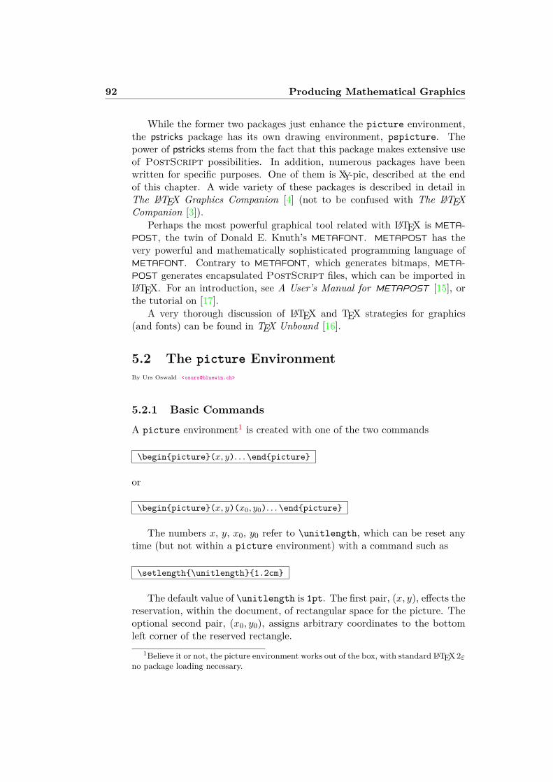
92 Producing Mathematical Graphics

While the former two packages just enhance the picture environment,the pstricks package has its own drawing environment, pspicture. Thepower of pstricks stems from the fact that this package makes extensive useof PostScript possibilities. In addition, numerous packages have beenwritten for specific purposes. One of them is XY-pic, described at the endof this chapter. A wide variety of these packages is described in detail inThe LATEX Graphics Companion [4] (not to be confused with The LATEXCompanion [3]).

Perhaps the most powerful graphical tool related with LATEX is META-POST, the twin of Donald E. Knuth’s METAFONT. METAPOST has thevery powerful and mathematically sophisticated programming language ofMETAFONT. Contrary to METAFONT, which generates bitmaps, META-POST generates encapsulated PostScript files, which can be imported inLATEX. For an introduction, see A User’s Manual for METAPOST [15], orthe tutorial on [17].

A very thorough discussion of LATEX and TEX strategies for graphics(and fonts) can be found in TEX Unbound [16].

5.2 The picture EnvironmentBy Urs Oswald <osurs@bluewin.ch>

5.2.1 Basic Commands

A picture environment1 is created with one of the two commands

\beginpicture(x, y). . . \endpicture

or

\beginpicture(x, y)(x0, y0). . . \endpicture

The numbers x, y, x0, y0 refer to \unitlength, which can be reset anytime (but not within a picture environment) with a command such as

\setlength\unitlength1.2cm

The default value of \unitlength is 1pt. The first pair, (x, y), effects thereservation, within the document, of rectangular space for the picture. Theoptional second pair, (x0, y0), assigns arbitrary coordinates to the bottomleft corner of the reserved rectangle.

1Believe it or not, the picture environment works out of the box, with standard LATEX2εno package loading necessary.

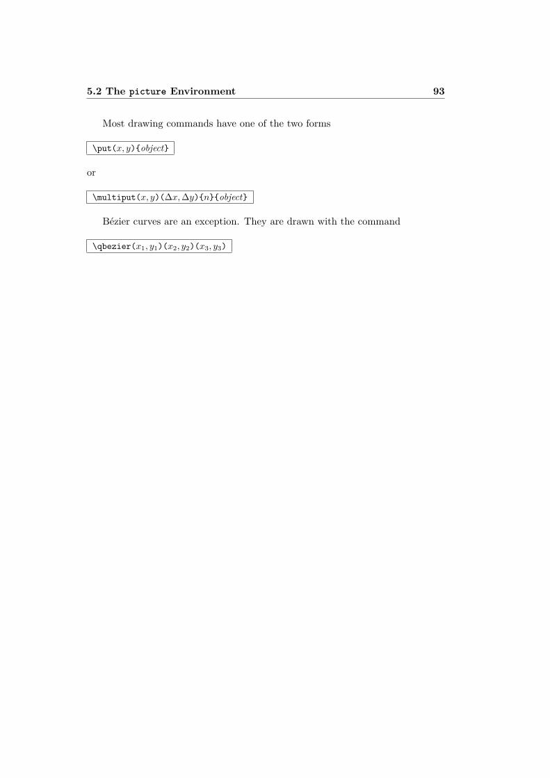
5.2 The picture Environment 93

Most drawing commands have one of the two forms

\put(x, y)object

or

\multiput(x, y)(∆x,∆y)nobject

Bézier curves are an exception. They are drawn with the command

\qbezier(x1, y1)(x2, y2)(x3, y3)

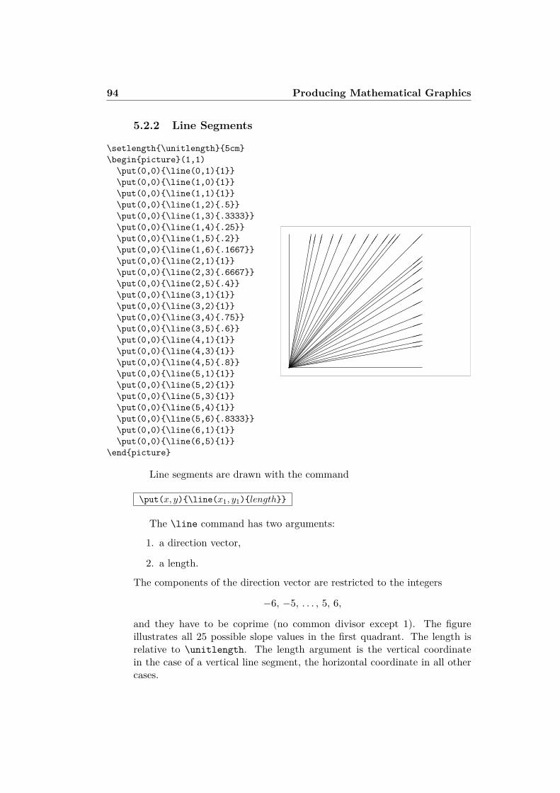
94 Producing Mathematical Graphics

5.2.2 Line Segments

\setlength\unitlength5cm\beginpicture(1,1)\put(0,0)\line(0,1)1\put(0,0)\line(1,0)1\put(0,0)\line(1,1)1\put(0,0)\line(1,2).5\put(0,0)\line(1,3).3333\put(0,0)\line(1,4).25\put(0,0)\line(1,5).2\put(0,0)\line(1,6).1667\put(0,0)\line(2,1)1\put(0,0)\line(2,3).6667\put(0,0)\line(2,5).4\put(0,0)\line(3,1)1\put(0,0)\line(3,2)1\put(0,0)\line(3,4).75\put(0,0)\line(3,5).6\put(0,0)\line(4,1)1\put(0,0)\line(4,3)1\put(0,0)\line(4,5).8\put(0,0)\line(5,1)1\put(0,0)\line(5,2)1\put(0,0)\line(5,3)1\put(0,0)\line(5,4)1\put(0,0)\line(5,6).8333\put(0,0)\line(6,1)1\put(0,0)\line(6,5)1

\endpicture

!!!!

!!!!

!!!!

!!!

"""""""""""""""

###############

%%%%%%%%%%%%%%%

(((((((

((((((((

,,,,,,,,,,,,,,,

Line segments are drawn with the command

\put(x, y)\line(x1, y1)length

The \line command has two arguments:

1. a direction vector,

2. a length.

The components of the direction vector are restricted to the integers

−6, −5, . . . , 5, 6,

and they have to be coprime (no common divisor except 1). The figureillustrates all 25 possible slope values in the first quadrant. The length isrelative to \unitlength. The length argument is the vertical coordinatein the case of a vertical line segment, the horizontal coordinate in all othercases.

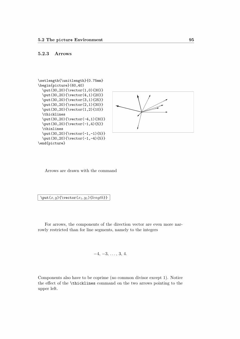
5.2 The picture Environment 95

5.2.3 Arrows

\setlength\unitlength0.75mm\beginpicture(60,40)\put(30,20)\vector(1,0)30\put(30,20)\vector(4,1)20\put(30,20)\vector(3,1)25\put(30,20)\vector(2,1)30\put(30,20)\vector(1,2)10\thicklines\put(30,20)\vector(-4,1)30\put(30,20)\vector(-1,4)5\thinlines\put(30,20)\vector(-1,-1)5\put(30,20)\vector(-1,-4)5

\endpicture

-:

1

*

XXXXXX

Xy

CCCCCO

Arrows are drawn with the command

\put(x, y)\vector(x1, y1)length

For arrows, the components of the direction vector are even more nar-rowly restricted than for line segments, namely to the integers

−4, −3, . . . , 3, 4.

Components also have to be coprime (no common divisor except 1). Noticethe effect of the \thicklines command on the two arrows pointing to theupper left.

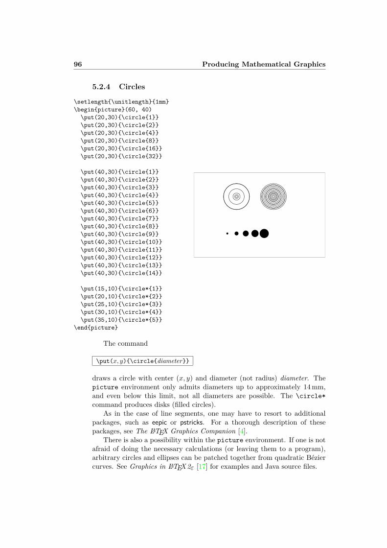
96 Producing Mathematical Graphics

5.2.4 Circles

\setlength\unitlength1mm\beginpicture(60, 40)\put(20,30)\circle1\put(20,30)\circle2\put(20,30)\circle4\put(20,30)\circle8\put(20,30)\circle16\put(20,30)\circle32

\put(40,30)\circle1\put(40,30)\circle2\put(40,30)\circle3\put(40,30)\circle4\put(40,30)\circle5\put(40,30)\circle6\put(40,30)\circle7\put(40,30)\circle8\put(40,30)\circle9\put(40,30)\circle10\put(40,30)\circle11\put(40,30)\circle12\put(40,30)\circle13\put(40,30)\circle14

\put(15,10)\circle*1\put(20,10)\circle*2\put(25,10)\circle*3\put(30,10)\circle*4\put(35,10)\circle*5

\endpicture

bej&%'$&%'$behjm "!# "!# &%'$

r u x z

The command

\put(x, y)\circlediameter

draws a circle with center (x, y) and diameter (not radius) diameter. Thepicture environment only admits diameters up to approximately 14mm,and even below this limit, not all diameters are possible. The \circle*command produces disks (filled circles).

As in the case of line segments, one may have to resort to additionalpackages, such as eepic or pstricks. For a thorough description of thesepackages, see The LATEX Graphics Companion [4].

There is also a possibility within the picture environment. If one is notafraid of doing the necessary calculations (or leaving them to a program),arbitrary circles and ellipses can be patched together from quadratic Béziercurves. See Graphics in LATEX2ε [17] for examples and Java source files.

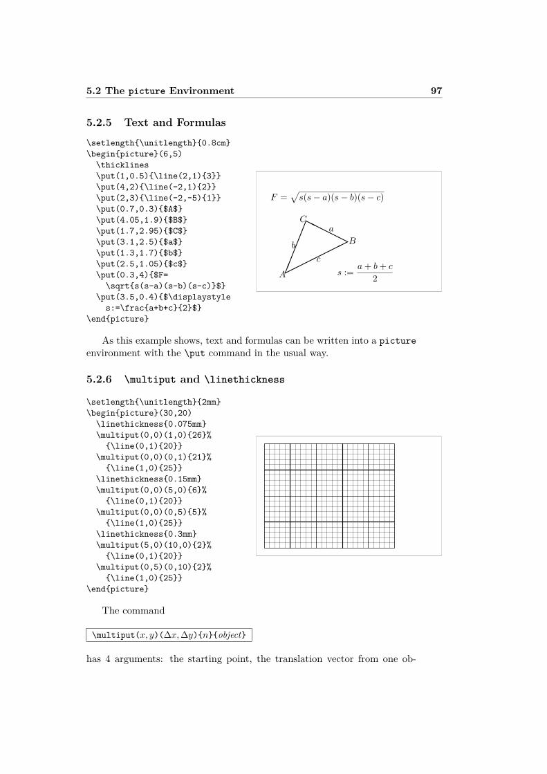
5.2 The picture Environment 97

5.2.5 Text and Formulas

\setlength\unitlength0.8cm\beginpicture(6,5)\thicklines\put(1,0.5)\line(2,1)3\put(4,2)\line(-2,1)2\put(2,3)\line(-2,-5)1\put(0.7,0.3)$A$\put(4.05,1.9)$B$\put(1.7,2.95)$C$\put(3.1,2.5)$a$\put(1.3,1.7)$b$\put(2.5,1.05)$c$\put(0.3,4)$F=\sqrts(s-a)(s-b)(s-c)$

\put(3.5,0.4)$\displaystyles:=\fraca+b+c2$

\endpicture

HH

HHHA

B

Ca

b

c

F =√s(s− a)(s− b)(s− c)

s := a+ b+ c

2

As this example shows, text and formulas can be written into a pictureenvironment with the \put command in the usual way.

5.2.6 \multiput and \linethickness

\setlength\unitlength2mm\beginpicture(30,20)\linethickness0.075mm\multiput(0,0)(1,0)26%\line(0,1)20

\multiput(0,0)(0,1)21%\line(1,0)25

\linethickness0.15mm\multiput(0,0)(5,0)6%\line(0,1)20

\multiput(0,0)(0,5)5%\line(1,0)25

\linethickness0.3mm\multiput(5,0)(10,0)2%\line(0,1)20

\multiput(0,5)(0,10)2%\line(1,0)25

\endpicture

The command

\multiput(x, y)(∆x,∆y)nobject

has 4 arguments: the starting point, the translation vector from one ob-

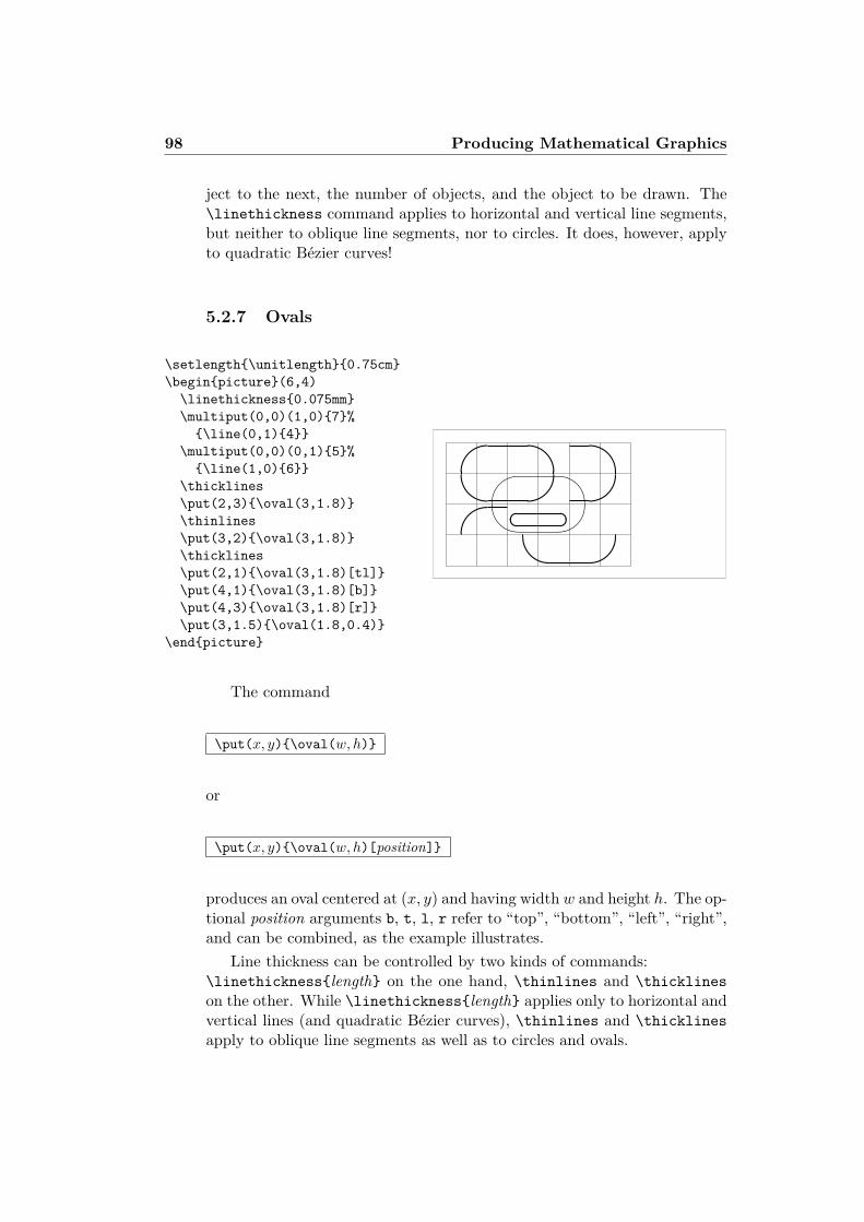
98 Producing Mathematical Graphics

ject to the next, the number of objects, and the object to be drawn. The\linethickness command applies to horizontal and vertical line segments,but neither to oblique line segments, nor to circles. It does, however, applyto quadratic Bézier curves!

5.2.7 Ovals

\setlength\unitlength0.75cm\beginpicture(6,4)\linethickness0.075mm\multiput(0,0)(1,0)7%\line(0,1)4

\multiput(0,0)(0,1)5%\line(1,0)6

\thicklines\put(2,3)\oval(3,1.8)\thinlines\put(3,2)\oval(3,1.8)\thicklines\put(2,1)\oval(3,1.8)[tl]\put(4,1)\oval(3,1.8)[b]\put(4,3)\oval(3,1.8)[r]\put(3,1.5)\oval(1.8,0.4)

\endpicture

#" !#

" !#

" !

!

The command

\put(x, y)\oval(w, h)

or

\put(x, y)\oval(w, h)[position]

produces an oval centered at (x, y) and having width w and height h. The op-tional position arguments b, t, l, r refer to “top”, “bottom”, “left”, “right”,and can be combined, as the example illustrates.

Line thickness can be controlled by two kinds of commands:\linethicknesslength on the one hand, \thinlines and \thicklineson the other. While \linethicknesslength applies only to horizontal andvertical lines (and quadratic Bézier curves), \thinlines and \thicklinesapply to oblique line segments as well as to circles and ovals.

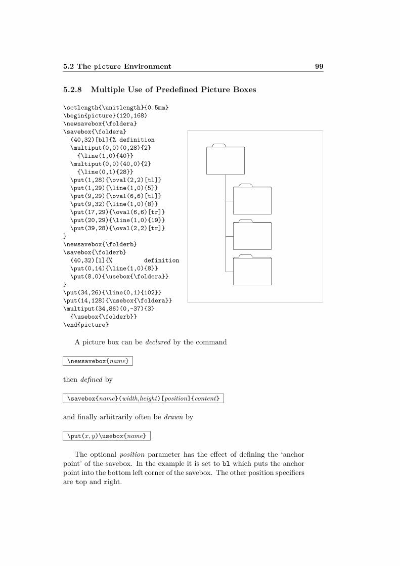
5.2 The picture Environment 99

5.2.8 Multiple Use of Predefined Picture Boxes

\setlength\unitlength0.5mm\beginpicture(120,168)\newsavebox\foldera\savebox\foldera(40,32)[bl]% definition\multiput(0,0)(0,28)2\line(1,0)40

\multiput(0,0)(40,0)2\line(0,1)28

\put(1,28)\oval(2,2)[tl]\put(1,29)\line(1,0)5\put(9,29)\oval(6,6)[tl]\put(9,32)\line(1,0)8\put(17,29)\oval(6,6)[tr]\put(20,29)\line(1,0)19\put(39,28)\oval(2,2)[tr]

\newsavebox\folderb\savebox\folderb(40,32)[l]% definition\put(0,14)\line(1,0)8\put(8,0)\usebox\foldera

\put(34,26)\line(0,1)102\put(14,128)\usebox\foldera\multiput(34,86)(0,-37)3\usebox\folderb

\endpicture

A picture box can be declared by the command

\newsaveboxname

then defined by

\saveboxname(width,height)[position]content

and finally arbitrarily often be drawn by

\put(x, y)\useboxname

The optional position parameter has the effect of defining the ‘anchorpoint’ of the savebox. In the example it is set to bl which puts the anchorpoint into the bottom left corner of the savebox. The other position specifiersare top and right.

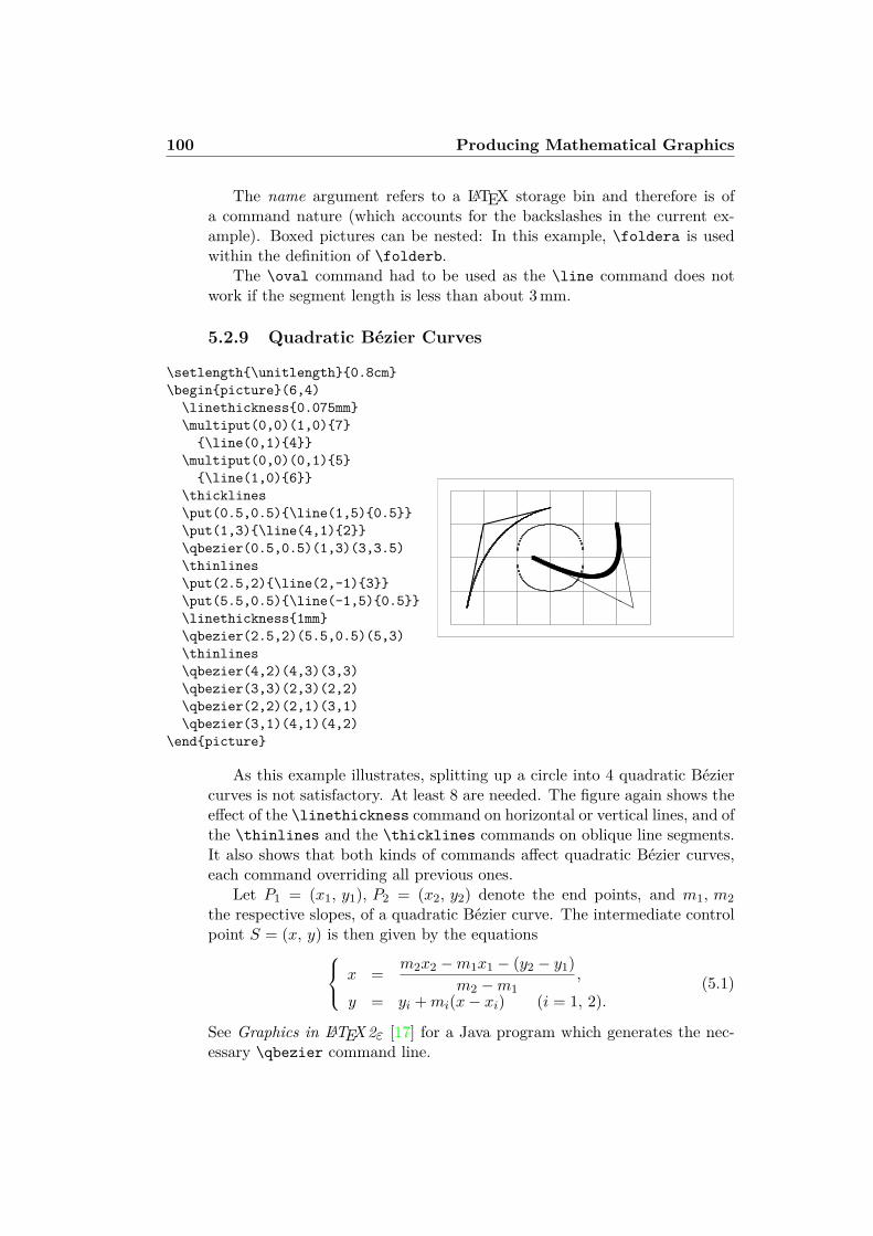
100 Producing Mathematical Graphics

The name argument refers to a LATEX storage bin and therefore is ofa command nature (which accounts for the backslashes in the current ex-ample). Boxed pictures can be nested: In this example, \foldera is usedwithin the definition of \folderb.

The \oval command had to be used as the \line command does notwork if the segment length is less than about 3mm.

5.2.9 Quadratic Bézier Curves

\setlength\unitlength0.8cm\beginpicture(6,4)\linethickness0.075mm\multiput(0,0)(1,0)7\line(0,1)4

\multiput(0,0)(0,1)5\line(1,0)6

\thicklines\put(0.5,0.5)\line(1,5)0.5\put(1,3)\line(4,1)2\qbezier(0.5,0.5)(1,3)(3,3.5)\thinlines\put(2.5,2)\line(2,-1)3\put(5.5,0.5)\line(-1,5)0.5\linethickness1mm\qbezier(2.5,2)(5.5,0.5)(5,3)\thinlines\qbezier(4,2)(4,3)(3,3)\qbezier(3,3)(2,3)(2,2)\qbezier(2,2)(2,1)(3,1)\qbezier(3,1)(4,1)(4,2)

\endpicture

HHHHHHHD

DDDDD

As this example illustrates, splitting up a circle into 4 quadratic Béziercurves is not satisfactory. At least 8 are needed. The figure again shows theeffect of the \linethickness command on horizontal or vertical lines, and ofthe \thinlines and the \thicklines commands on oblique line segments.It also shows that both kinds of commands affect quadratic Bézier curves,each command overriding all previous ones.

Let P1 = (x1, y1), P2 = (x2, y2) denote the end points, and m1, m2the respective slopes, of a quadratic Bézier curve. The intermediate controlpoint S = (x, y) is then given by the equations x = m2x2 −m1x1 − (y2 − y1)

m2 −m1,

y = yi +mi(x− xi) (i = 1, 2).(5.1)

See Graphics in LATEX2ε [17] for a Java program which generates the nec-essary \qbezier command line.

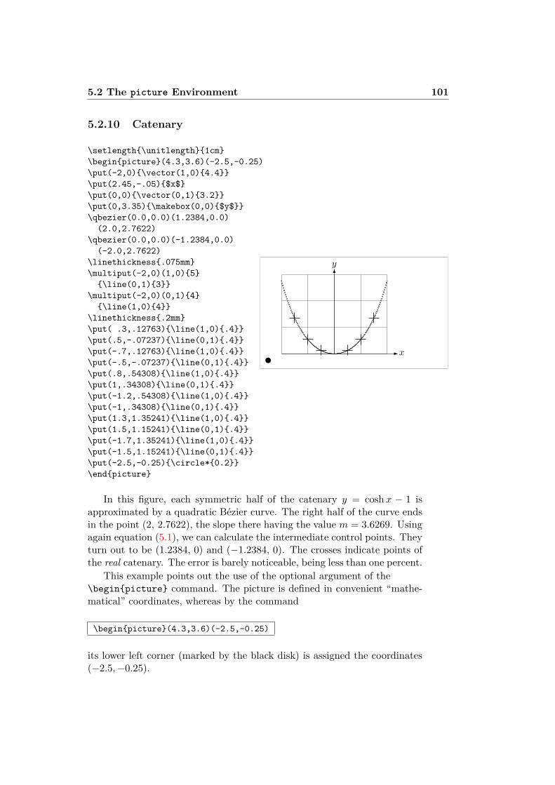
5.2 The picture Environment 101

5.2.10 Catenary

\setlength\unitlength1cm\beginpicture(4.3,3.6)(-2.5,-0.25)\put(-2,0)\vector(1,0)4.4\put(2.45,-.05)$x$\put(0,0)\vector(0,1)3.2\put(0,3.35)\makebox(0,0)$y$\qbezier(0.0,0.0)(1.2384,0.0)(2.0,2.7622)

\qbezier(0.0,0.0)(-1.2384,0.0)(-2.0,2.7622)

\linethickness.075mm\multiput(-2,0)(1,0)5\line(0,1)3

\multiput(-2,0)(0,1)4\line(1,0)4

\linethickness.2mm\put( .3,.12763)\line(1,0).4\put(.5,-.07237)\line(0,1).4\put(-.7,.12763)\line(1,0).4\put(-.5,-.07237)\line(0,1).4\put(.8,.54308)\line(1,0).4\put(1,.34308)\line(0,1).4\put(-1.2,.54308)\line(1,0).4\put(-1,.34308)\line(0,1).4\put(1.3,1.35241)\line(1,0).4\put(1.5,1.15241)\line(0,1).4\put(-1.7,1.35241)\line(1,0).4\put(-1.5,1.15241)\line(0,1).4\put(-2.5,-0.25)\circle*0.2\endpicture

-x

6

y

u

In this figure, each symmetric half of the catenary y = cosh x − 1 isapproximated by a quadratic Bézier curve. The right half of the curve endsin the point (2, 2.7622), the slope there having the value m = 3.6269. Usingagain equation (5.1), we can calculate the intermediate control points. Theyturn out to be (1.2384, 0) and (−1.2384, 0). The crosses indicate points ofthe real catenary. The error is barely noticeable, being less than one percent.

This example points out the use of the optional argument of the\beginpicture command. The picture is defined in convenient “mathe-matical” coordinates, whereas by the command

\beginpicture(4.3,3.6)(-2.5,-0.25)

its lower left corner (marked by the black disk) is assigned the coordinates(−2.5,−0.25).

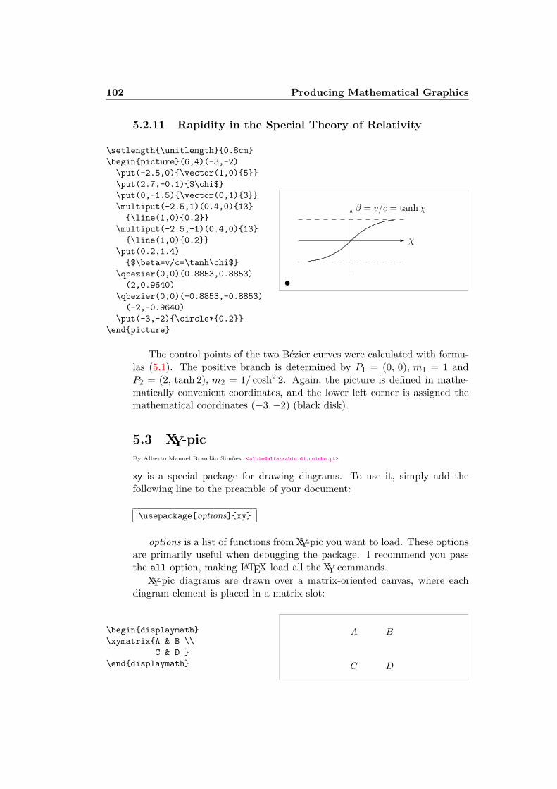
102 Producing Mathematical Graphics

5.2.11 Rapidity in the Special Theory of Relativity

\setlength\unitlength0.8cm\beginpicture(6,4)(-3,-2)\put(-2.5,0)\vector(1,0)5\put(2.7,-0.1)$\chi$\put(0,-1.5)\vector(0,1)3\multiput(-2.5,1)(0.4,0)13\line(1,0)0.2

\multiput(-2.5,-1)(0.4,0)13\line(1,0)0.2

\put(0.2,1.4)$\beta=v/c=\tanh\chi$

\qbezier(0,0)(0.8853,0.8853)(2,0.9640)

\qbezier(0,0)(-0.8853,-0.8853)(-2,-0.9640)

\put(-3,-2)\circle*0.2\endpicture

- χ

6β = v/c = tanhχ

t

The control points of the two Bézier curves were calculated with formu-las (5.1). The positive branch is determined by P1 = (0, 0), m1 = 1 andP2 = (2, tanh 2), m2 = 1/ cosh2 2. Again, the picture is defined in mathe-matically convenient coordinates, and the lower left corner is assigned themathematical coordinates (−3,−2) (black disk).

5.3 XY-picBy Alberto Manuel Brandão Simões <albie@alfarrabio.di.uminho.pt>

xy is a special package for drawing diagrams. To use it, simply add thefollowing line to the preamble of your document:

\usepackage[options]xy

options is a list of functions fromXY-pic you want to load. These optionsare primarily useful when debugging the package. I recommend you passthe all option, making LATEX load all the XY commands.

XY-pic diagrams are drawn over a matrix-oriented canvas, where eachdiagram element is placed in a matrix slot:

\begindisplaymath\xymatrixA & B \\

C & D \enddisplaymath

A B

C D

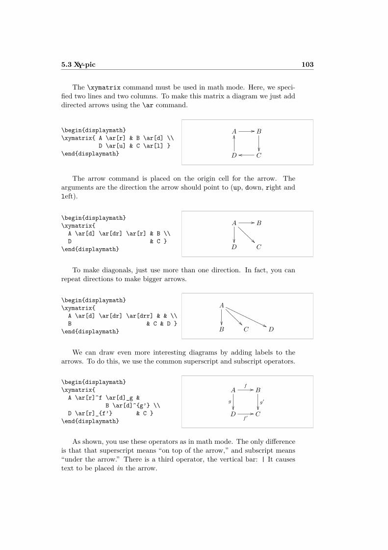
5.3 XY-pic 103

The \xymatrix command must be used in math mode. Here, we speci-fied two lines and two columns. To make this matrix a diagram we just adddirected arrows using the \ar command.

\begindisplaymath\xymatrix A \ar[r] & B \ar[d] \\

D \ar[u] & C \ar[l] \enddisplaymath

A // B

D

OO

Coo

The arrow command is placed on the origin cell for the arrow. Thearguments are the direction the arrow should point to (up, down, right andleft).

\begindisplaymath\xymatrixA \ar[d] \ar[dr] \ar[r] & B \\D & C

\enddisplaymath

A

@@@@@@@// B

D C

To make diagonals, just use more than one direction. In fact, you canrepeat directions to make bigger arrows.

\begindisplaymath\xymatrixA \ar[d] \ar[dr] \ar[drr] & & \\B & C & D

\enddisplaymath

A

@@@@@@@

''PPPPPPPPPPPPPP

B C D

We can draw even more interesting diagrams by adding labels to thearrows. To do this, we use the common superscript and subscript operators.

\begindisplaymath\xymatrixA \ar[r]^f \ar[d]_g &

B \ar[d]^g’ \\D \ar[r]_f’ & C

\enddisplaymath

Af //

g

B

g′

D

f ′// C

As shown, you use these operators as in math mode. The only differenceis that that superscript means “on top of the arrow,” and subscript means“under the arrow.” There is a third operator, the vertical bar: | It causestext to be placed in the arrow.

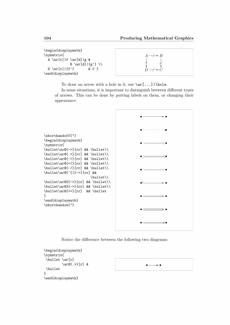
104 Producing Mathematical Graphics

\begindisplaymath\xymatrixA \ar[r]|f \ar[d]|g &

B \ar[d]|g’ \\D \ar[r]|f’ & C

\enddisplaymath

A f //

g

B

g′

D f ′ // C

To draw an arrow with a hole in it, use \ar[...]|\hole.In some situations, it is important to distinguish between different types

of arrows. This can be done by putting labels on them, or changing theirappearance:

\shorthandoff"\begindisplaymath\xymatrix\bullet\ar@->[rr] && \bullet\\\bullet\ar@.<[rr] && \bullet\\\bullet\ar@~)[rr] && \bullet\\\bullet\ar@=([rr] && \bullet\\\bullet\ar@~/[rr] && \bullet\\\bullet\ar@^(->[rr] &&

\bullet\\\bullet\ar@2->[rr] && \bullet\\\bullet\ar@3->[rr] && \bullet\\\bullet\ar@=+[rr] && \bullet\enddisplaymath\shorthandon"

• // •

• oo •

• _?/o/o/o/o/o/o/o •

• •

• /o/o/o/o/o/o/o •

• // •

• +3 •

• _*4 •

• _•

Notice the difference between the following two diagrams:

\begindisplaymath\xymatrix\bullet \ar[r]

\ar@.>[r] &\bullet\enddisplaymath

• //// •

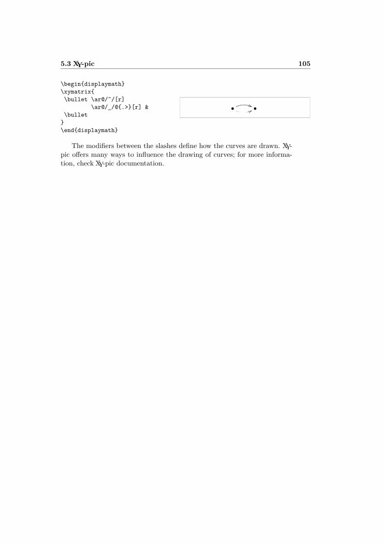
5.3 XY-pic 105

\begindisplaymath\xymatrix\bullet \ar@/^/[r]

\ar@/_/@.>[r] &\bullet\enddisplaymath

• ((66 •

The modifiers between the slashes define how the curves are drawn. XY-pic offers many ways to influence the drawing of curves; for more informa-tion, check XY-pic documentation.

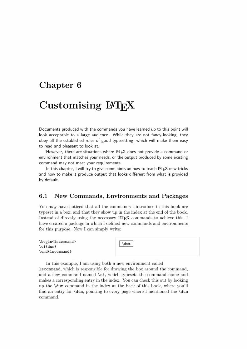
Chapter 6

Customising LATEX

Documents produced with the commands you have learned up to this point willlook acceptable to a large audience. While they are not fancy-looking, theyobey all the established rules of good typesetting, which will make them easyto read and pleasant to look at.

However, there are situations where LATEX does not provide a command orenvironment that matches your needs, or the output produced by some existingcommand may not meet your requirements.

In this chapter, I will try to give some hints on how to teach LATEX new tricksand how to make it produce output that looks different from what is providedby default.

6.1 New Commands, Environments and PackagesYou may have noticed that all the commands I introduce in this book aretypeset in a box, and that they show up in the index at the end of the book.Instead of directly using the necessary LATEX commands to achieve this, Ihave created a package in which I defined new commands and environmentsfor this purpose. Now I can simply write:

\beginlscommand\cidum\endlscommand

\dum

In this example, I am using both a new environment calledlscommand, which is responsible for drawing the box around the command,and a new command named \ci, which typesets the command name andmakes a corresponding entry in the index. You can check this out by lookingup the \dum command in the index at the back of this book, where you’llfind an entry for \dum, pointing to every page where I mentioned the \dumcommand.

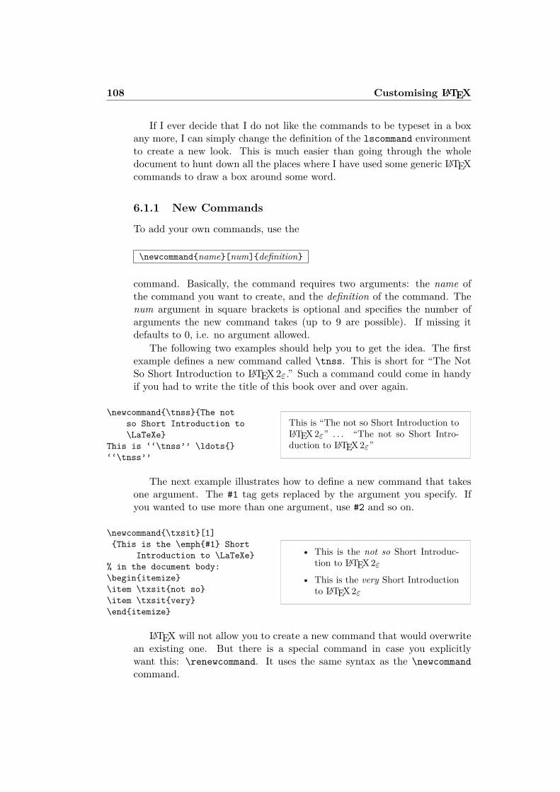
108 Customising LATEX

If I ever decide that I do not like the commands to be typeset in a boxany more, I can simply change the definition of the lscommand environmentto create a new look. This is much easier than going through the wholedocument to hunt down all the places where I have used some generic LATEXcommands to draw a box around some word.

6.1.1 New Commands

To add your own commands, use the

\newcommandname[num]definition

command. Basically, the command requires two arguments: the name ofthe command you want to create, and the definition of the command. Thenum argument in square brackets is optional and specifies the number ofarguments the new command takes (up to 9 are possible). If missing itdefaults to 0, i.e. no argument allowed.

The following two examples should help you to get the idea. The firstexample defines a new command called \tnss. This is short for “The NotSo Short Introduction to LATEX2ε.” Such a command could come in handyif you had to write the title of this book over and over again.

\newcommand\tnssThe notso Short Introduction to\LaTeXe

This is ‘‘\tnss’’ \ldots‘‘\tnss’’

This is “The not so Short Introduction toLATEX2ε” . . . “The not so Short Intro-duction to LATEX2ε”

The next example illustrates how to define a new command that takesone argument. The #1 tag gets replaced by the argument you specify. Ifyou wanted to use more than one argument, use #2 and so on.

\newcommand\txsit[1]This is the \emph#1 Short

Introduction to \LaTeXe% in the document body:\beginitemize\item \txsitnot so\item \txsitvery\enditemize

• This is the not so Short Introduc-tion to LATEX2ε

• This is the very Short Introductionto LATEX2ε

LATEX will not allow you to create a new command that would overwritean existing one. But there is a special command in case you explicitlywant this: \renewcommand. It uses the same syntax as the \newcommandcommand.

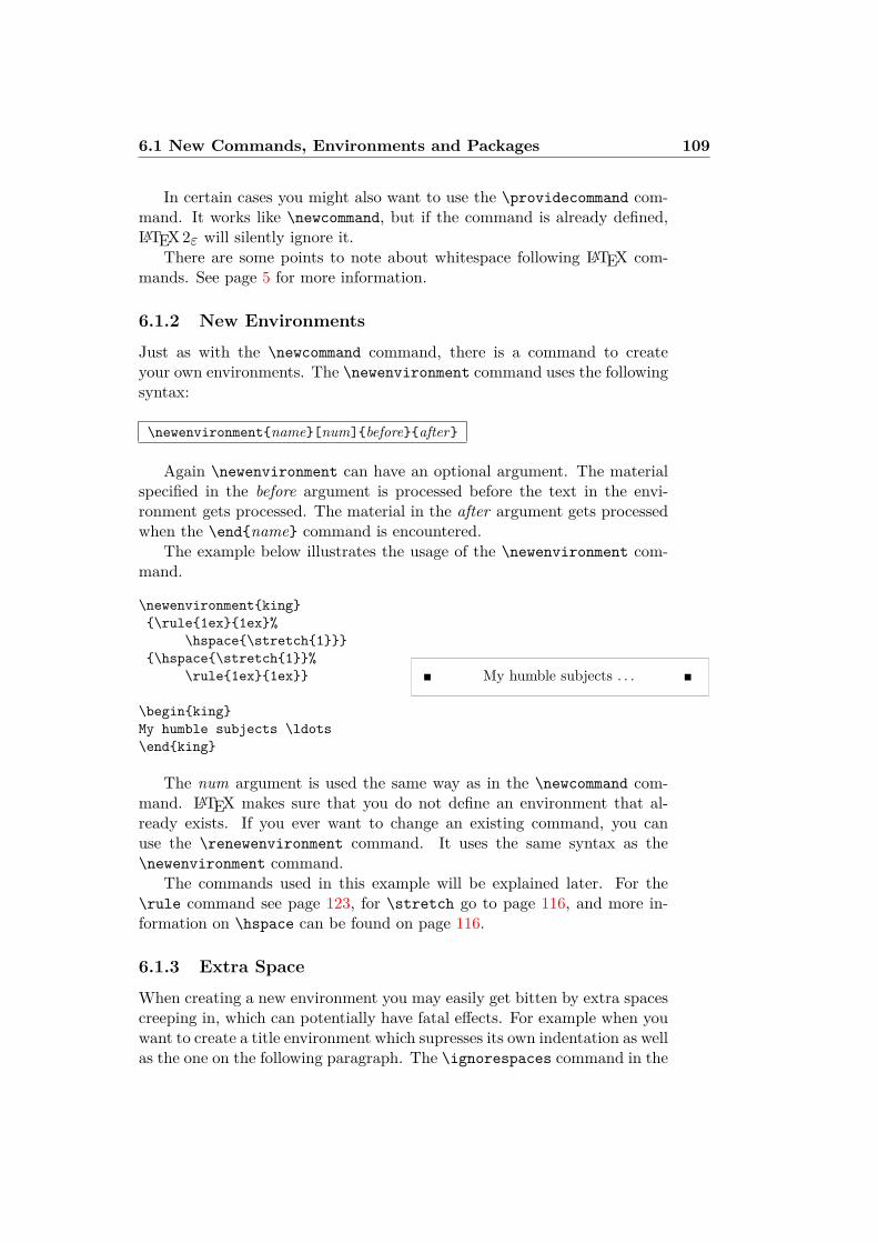
6.1 New Commands, Environments and Packages 109

In certain cases you might also want to use the \providecommand com-mand. It works like \newcommand, but if the command is already defined,LATEX2ε will silently ignore it.

There are some points to note about whitespace following LATEX com-mands. See page 5 for more information.

6.1.2 New Environments

Just as with the \newcommand command, there is a command to createyour own environments. The \newenvironment command uses the followingsyntax:

\newenvironmentname[num]beforeafter

Again \newenvironment can have an optional argument. The materialspecified in the before argument is processed before the text in the envi-ronment gets processed. The material in the after argument gets processedwhen the \endname command is encountered.

The example below illustrates the usage of the \newenvironment com-mand.

\newenvironmentking\rule1ex1ex%

\hspace\stretch1\hspace\stretch1%

\rule1ex1ex

\beginkingMy humble subjects \ldots\endking

My humble subjects . . .

The num argument is used the same way as in the \newcommand com-mand. LATEX makes sure that you do not define an environment that al-ready exists. If you ever want to change an existing command, you canuse the \renewenvironment command. It uses the same syntax as the\newenvironment command.

The commands used in this example will be explained later. For the\rule command see page 123, for \stretch go to page 116, and more in-formation on \hspace can be found on page 116.

6.1.3 Extra Space

When creating a new environment you may easily get bitten by extra spacescreeping in, which can potentially have fatal effects. For example when youwant to create a title environment which supresses its own indentation as wellas the one on the following paragraph. The \ignorespaces command in the

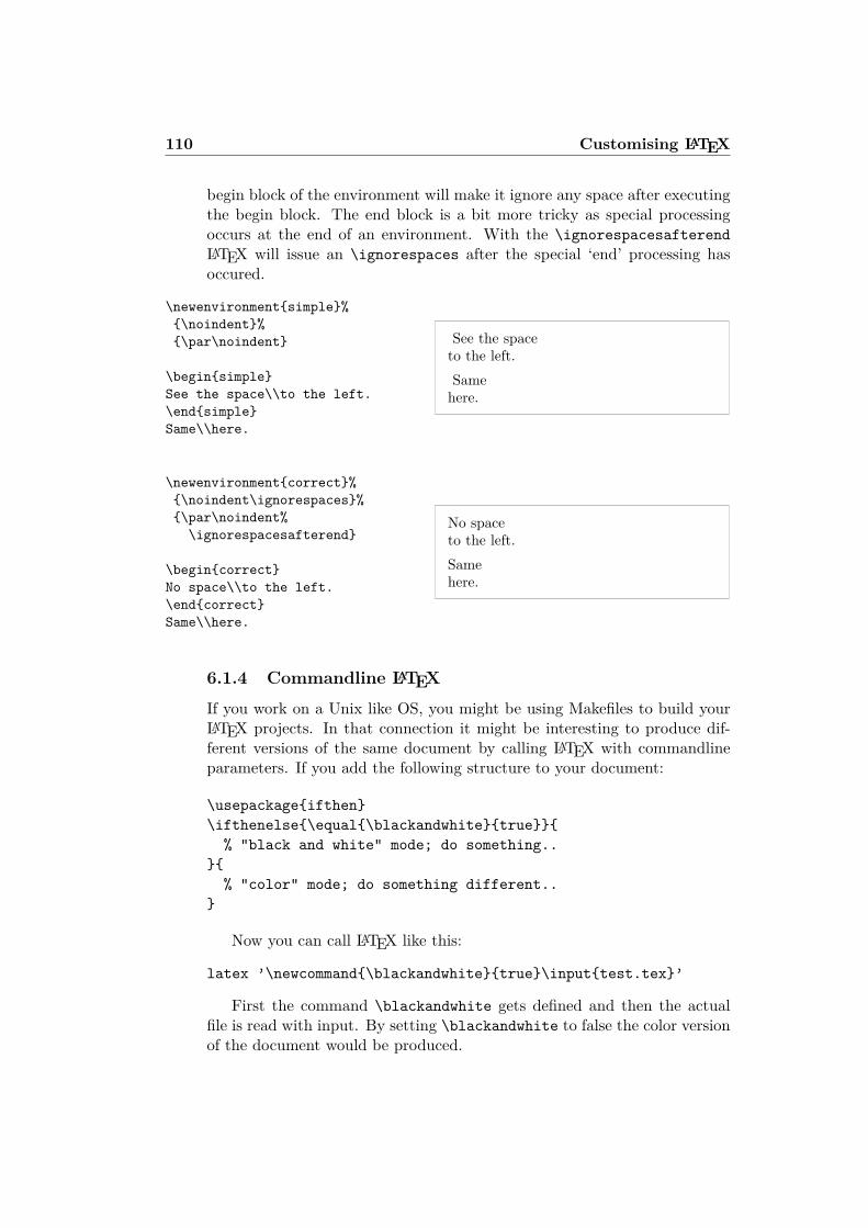
110 Customising LATEX

begin block of the environment will make it ignore any space after executingthe begin block. The end block is a bit more tricky as special processingoccurs at the end of an environment. With the \ignorespacesafterendLATEX will issue an \ignorespaces after the special ‘end’ processing hasoccured.

\newenvironmentsimple%\noindent%\par\noindent

\beginsimpleSee the space\\to the left.\endsimpleSame\\here.

See the spaceto the left.Samehere.

\newenvironmentcorrect%\noindent\ignorespaces%\par\noindent%

\ignorespacesafterend

\begincorrectNo space\\to the left.\endcorrectSame\\here.

No spaceto the left.Samehere.

6.1.4 Commandline LATEX

If you work on a Unix like OS, you might be using Makefiles to build yourLATEX projects. In that connection it might be interesting to produce dif-ferent versions of the same document by calling LATEX with commandlineparameters. If you add the following structure to your document:

\usepackageifthen\ifthenelse\equal\blackandwhitetrue

% "black and white" mode; do something..

% "color" mode; do something different..

Now you can call LATEX like this:

latex ’\newcommand\blackandwhitetrue\inputtest.tex’

First the command \blackandwhite gets defined and then the actualfile is read with input. By setting \blackandwhite to false the color versionof the document would be produced.

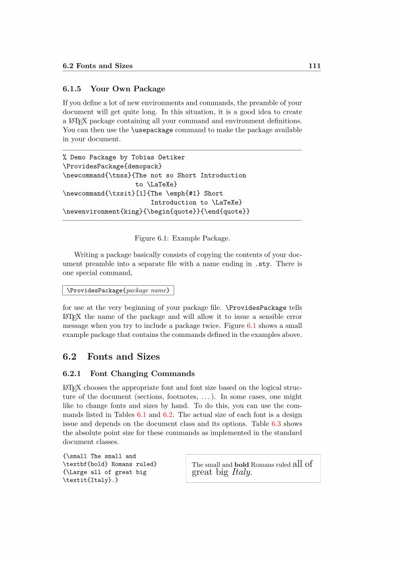
6.2 Fonts and Sizes 111

6.1.5 Your Own Package

If you define a lot of new environments and commands, the preamble of yourdocument will get quite long. In this situation, it is a good idea to createa LATEX package containing all your command and environment definitions.You can then use the \usepackage command to make the package availablein your document.

% Demo Package by Tobias Oetiker\ProvidesPackagedemopack\newcommand\tnssThe not so Short Introduction

to \LaTeXe\newcommand\txsit[1]The \emph#1 Short

Introduction to \LaTeXe\newenvironmentking\beginquote\endquote

Figure 6.1: Example Package.

Writing a package basically consists of copying the contents of your doc-ument preamble into a separate file with a name ending in .sty. There isone special command,

\ProvidesPackagepackage name

for use at the very beginning of your package file. \ProvidesPackage tellsLATEX the name of the package and will allow it to issue a sensible errormessage when you try to include a package twice. Figure 6.1 shows a smallexample package that contains the commands defined in the examples above.

6.2 Fonts and Sizes

6.2.1 Font Changing Commands

LATEX chooses the appropriate font and font size based on the logical struc-ture of the document (sections, footnotes, . . . ). In some cases, one mightlike to change fonts and sizes by hand. To do this, you can use the com-mands listed in Tables 6.1 and 6.2. The actual size of each font is a designissue and depends on the document class and its options. Table 6.3 showsthe absolute point size for these commands as implemented in the standarddocument classes.

\small The small and\textbfbold Romans ruled\Large all of great big\textitItaly.

The small and bold Romans ruled all ofgreat big Italy.

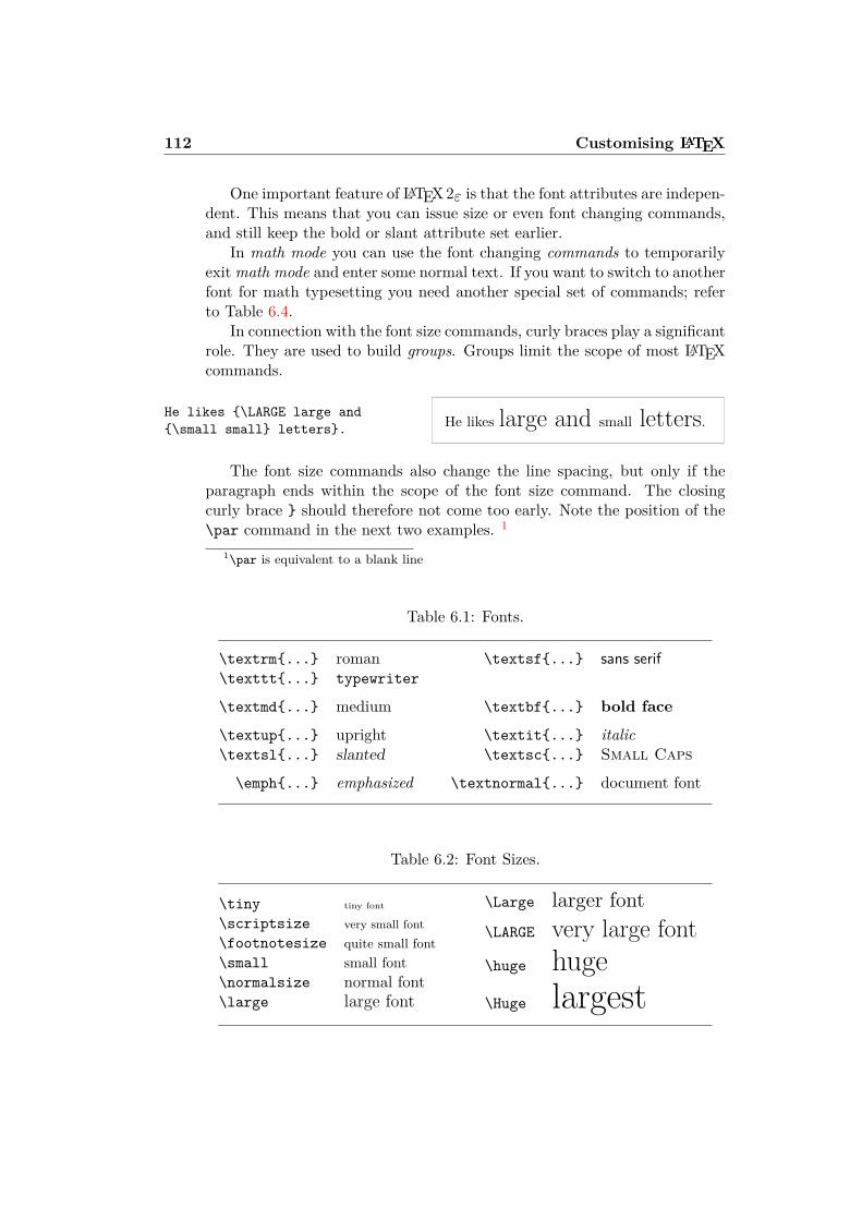
112 Customising LATEX

One important feature of LATEX2ε is that the font attributes are indepen-dent. This means that you can issue size or even font changing commands,and still keep the bold or slant attribute set earlier.

In math mode you can use the font changing commands to temporarilyexitmath mode and enter some normal text. If you want to switch to anotherfont for math typesetting you need another special set of commands; referto Table 6.4.

In connection with the font size commands, curly braces play a significantrole. They are used to build groups. Groups limit the scope of most LATEXcommands.

He likes \LARGE large and\small small letters. He likes large and small letters.

The font size commands also change the line spacing, but only if theparagraph ends within the scope of the font size command. The closingcurly brace should therefore not come too early. Note the position of the\par command in the next two examples. 1

1\par is equivalent to a blank line

Table 6.1: Fonts.

\textrm... roman \textsf... sans serif\texttt... typewriter

\textmd... medium \textbf... bold face

\textup... upright \textit... italic\textsl... slanted \textsc... Small Caps

\emph... emphasized \textnormal... document font

Table 6.2: Font Sizes.

\tiny tiny font

\scriptsize very small font\footnotesize quite small font\small small font\normalsize normal font\large large font

\Large larger font\LARGE very large font\huge huge\Huge largest

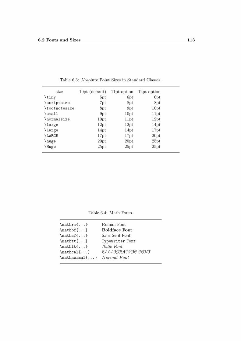
6.2 Fonts and Sizes 113

Table 6.3: Absolute Point Sizes in Standard Classes.

size 10pt (default) 11pt option 12pt option\tiny 5pt 6pt 6pt\scriptsize 7pt 8pt 8pt\footnotesize 8pt 9pt 10pt\small 9pt 10pt 11pt\normalsize 10pt 11pt 12pt\large 12pt 12pt 14pt\Large 14pt 14pt 17pt\LARGE 17pt 17pt 20pt\huge 20pt 20pt 25pt\Huge 25pt 25pt 25pt

Table 6.4: Math Fonts.

\mathrm... Roman Font\mathbf... Boldface Font\mathsf... Sans Serif Font\mathtt... Typewriter Font\mathit... Italic Font\mathcal... CALLIGRAPHIC FONT

\mathnormal... Normal Font

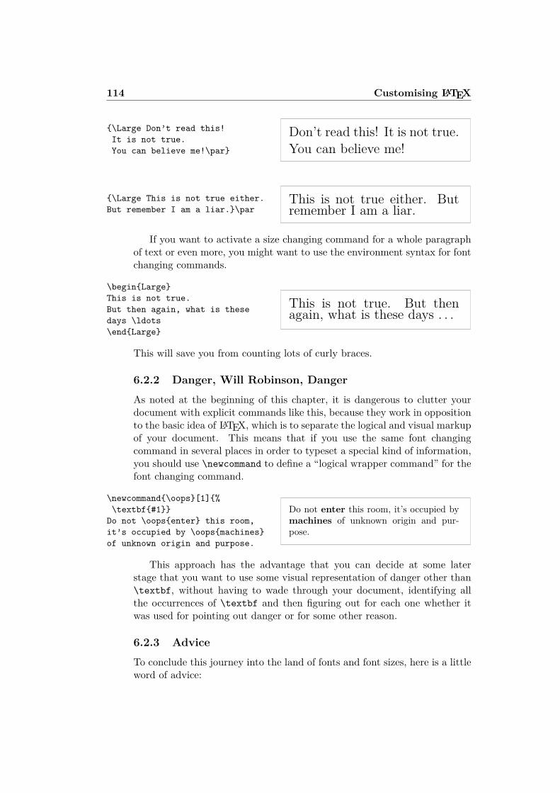
114 Customising LATEX

\Large Don’t read this!It is not true.You can believe me!\par

Don’t read this! It is not true.You can believe me!

\Large This is not true either.But remember I am a liar.\par

This is not true either. Butremember I am a liar.

If you want to activate a size changing command for a whole paragraphof text or even more, you might want to use the environment syntax for fontchanging commands.

\beginLargeThis is not true.But then again, what is thesedays \ldots\endLarge

This is not true. But thenagain, what is these days . . .

This will save you from counting lots of curly braces.

6.2.2 Danger, Will Robinson, Danger

As noted at the beginning of this chapter, it is dangerous to clutter yourdocument with explicit commands like this, because they work in oppositionto the basic idea of LATEX, which is to separate the logical and visual markupof your document. This means that if you use the same font changingcommand in several places in order to typeset a special kind of information,you should use \newcommand to define a “logical wrapper command” for thefont changing command.

\newcommand\oops[1]%\textbf#1Do not \oopsenter this room,it’s occupied by \oopsmachinesof unknown origin and purpose.

Do not enter this room, it’s occupied bymachines of unknown origin and pur-pose.

This approach has the advantage that you can decide at some laterstage that you want to use some visual representation of danger other than\textbf, without having to wade through your document, identifying allthe occurrences of \textbf and then figuring out for each one whether itwas used for pointing out danger or for some other reason.

6.2.3 Advice

To conclude this journey into the land of fonts and font sizes, here is a littleword of advice:

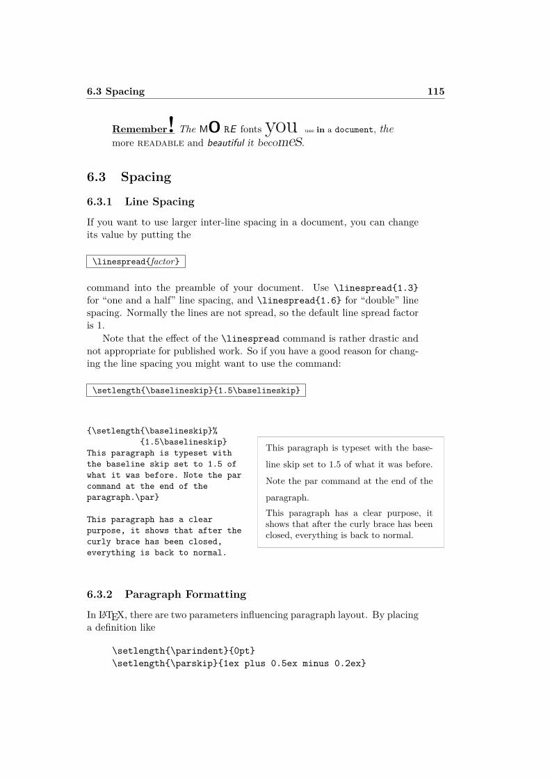
6.3 Spacing 115

Remember! The MO RE fonts you use in a document, themore readable and beautiful it becomes.

6.3 Spacing

6.3.1 Line Spacing

If you want to use larger inter-line spacing in a document, you can changeits value by putting the

\linespreadfactor

command into the preamble of your document. Use \linespread1.3for “one and a half” line spacing, and \linespread1.6 for “double” linespacing. Normally the lines are not spread, so the default line spread factoris 1.

Note that the effect of the \linespread command is rather drastic andnot appropriate for published work. So if you have a good reason for chang-ing the line spacing you might want to use the command:

\setlength\baselineskip1.5\baselineskip

\setlength\baselineskip%1.5\baselineskip

This paragraph is typeset withthe baseline skip set to 1.5 ofwhat it was before. Note the parcommand at the end of theparagraph.\par

This paragraph has a clearpurpose, it shows that after thecurly brace has been closed,everything is back to normal.

This paragraph is typeset with the base-

line skip set to 1.5 of what it was before.

Note the par command at the end of the

paragraph.This paragraph has a clear purpose, itshows that after the curly brace has beenclosed, everything is back to normal.

6.3.2 Paragraph Formatting

In LATEX, there are two parameters influencing paragraph layout. By placinga definition like

\setlength\parindent0pt\setlength\parskip1ex plus 0.5ex minus 0.2ex

116 Customising LATEX

in the preamble of the input file, you can change the layout of paragraphs.These two commands increase the space between two paragraphs while set-ting the paragraph indent to zero.

The plus and minus parts of the length above tell TEX that it cancompress and expand the inter paragraph skip by the amount specified, ifthis is necessary to properly fit the paragraphs onto the page.

In continental Europe, paragraphs are often separated by some space andnot indented. But beware, this also has its effect on the table of contents.Its lines get spaced more loosely now as well. To avoid this, you mightwant to move the two commands from the preamble into your document tosome place below the command \tableofcontents or to not use them atall, because you’ll find that most professional books use indenting and notspacing to separate paragraphs.

If you want to indent a paragraph that is not indented, you can use

\indent

at the beginning of the paragraph.2 Obviously, this will only have an effectwhen \parindent is not set to zero.

To create a non-indented paragraph, you can use

\noindent

as the first command of the paragraph. This might come in handy whenyou start a document with body text and not with a sectioning command.

6.3.3 Horizontal Space

LATEX determines the spaces between words and sentences automatically.To add horizontal space, use:

\hspacelength

If such a space should be kept even if it falls at the end or the start ofa line, use \hspace* instead of \hspace. The length in the simplest case isjust a number plus a unit. The most important units are listed in Table 6.5.

This\hspace1.5cmis a spaceof 1.5 cm.

This is a space of 1.5 cm.

2To indent the first paragraph after each section head, use the indentfirst package inthe ‘tools’ bundle.

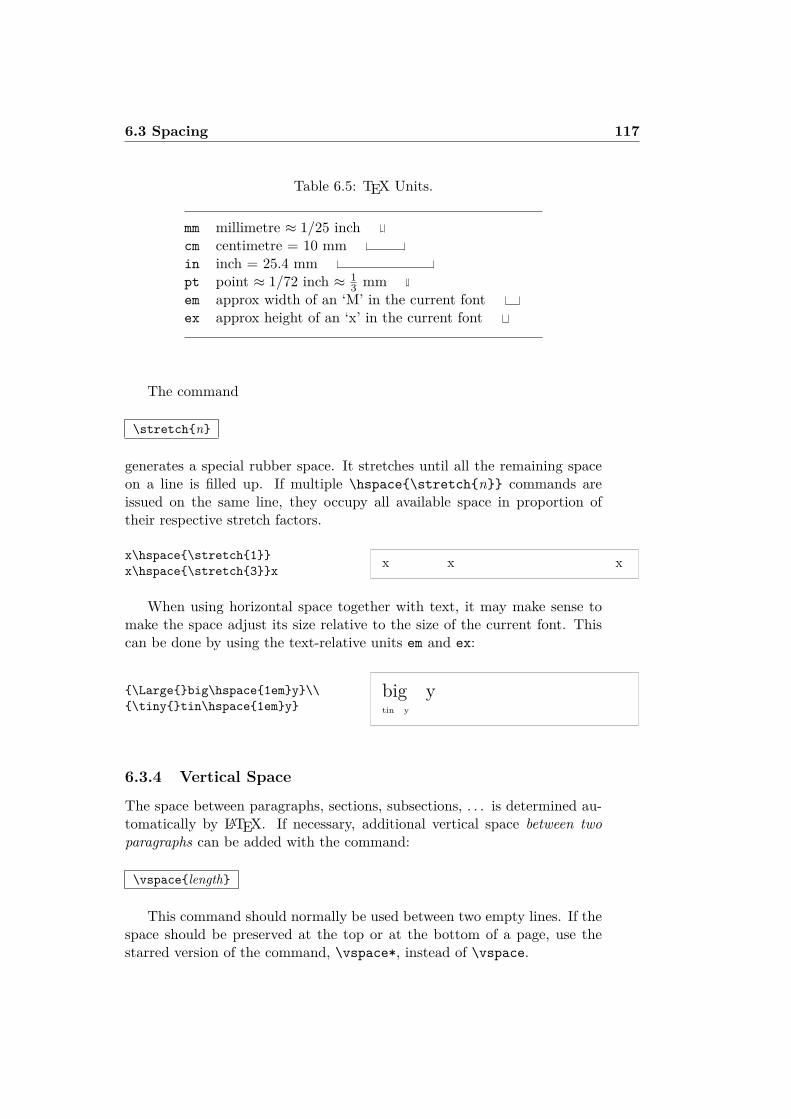
6.3 Spacing 117

Table 6.5: TEX Units.

mm millimetre ≈ 1/25 inchcm centimetre = 10 mmin inch = 25.4 mmpt point ≈ 1/72 inch ≈ 1

3 mmem approx width of an ‘M’ in the current fontex approx height of an ‘x’ in the current font

The command

\stretchn

generates a special rubber space. It stretches until all the remaining spaceon a line is filled up. If multiple \hspace\stretchn commands areissued on the same line, they occupy all available space in proportion oftheir respective stretch factors.

x\hspace\stretch1x\hspace\stretch3x

x x x

When using horizontal space together with text, it may make sense tomake the space adjust its size relative to the size of the current font. Thiscan be done by using the text-relative units em and ex:

\Largebig\hspace1emy\\\tinytin\hspace1emy

big ytin y

6.3.4 Vertical Space

The space between paragraphs, sections, subsections, . . . is determined au-tomatically by LATEX. If necessary, additional vertical space between twoparagraphs can be added with the command:

\vspacelength

This command should normally be used between two empty lines. If thespace should be preserved at the top or at the bottom of a page, use thestarred version of the command, \vspace*, instead of \vspace.

118 Customising LATEX

The \stretch command, in connection with \pagebreak, can be usedto typeset text on the last line of a page, or to centre text vertically on apage.

Some text \ldots

\vspace\stretch1This goes onto the last line of the page.\pagebreak

Additional space between two lines of the same paragraph or within atable is specified with the

\\[length]

command.With \bigskip and \smallskip you can skip a predefined amount of

vertical space without having to worry about exact numbers.

6.4 Page LayoutLATEX2ε allows you to specify the paper size in the \documentclass com-mand. It then automatically picks the right text margins, but sometimesyou may not be happy with the predefined values. Naturally, you can changethem. Figure 6.2 shows all the parameters that can be changed. The figurewas produced with the layout package from the tools bundle.3

WAIT! . . . before you launch into a “Let’s make that narrow page a bitwider” frenzy, take a few seconds to think. As with most things in LATEX,there is a good reason for the page layout to be as it is.

Sure, compared to your off-the-shelf MS Word page, it looks awfullynarrow. But take a look at your favourite book4 and count the number ofcharacters on a standard text line. You will find that there are no more thanabout 66 characters on each line. Now do the same on your LATEX page. Youwill find that there are also about 66 characters per line. Experience showsthat the reading gets difficult as soon as there are more characters on asingle line. This is because it is difficult for the eyes to move from the endof one line to the start of the next one. This is also why newspapers aretypeset in multiple columns.

So if you increase the width of your body text, keep in mind that youare making life difficult for the readers of your paper. But enough of thecautioning, I promised to tell you how you do it . . .

LATEX provides two commands to change these parameters. They areusually used in the document preamble.

3macros/latex/required/tools4I mean a real printed book produced by a reputable publisher.

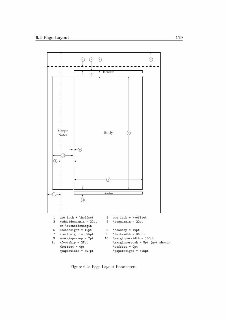
6.4 Page Layout 119

Header

Body

Footer

MarginNotes

i8 -

i7

?

6

i1 -

-i3 i10 -

- i9

6

?

i11

i2?

6i46

?

i56

?

i6

6

?

1 one inch + \hoffset 2 one inch + \voffset3 \oddsidemargin = 22pt 4 \topmargin = 22pt

or \evensidemargin5 \headheight = 12pt 6 \headsep = 19pt7 \textheight = 595pt 8 \textwidth = 360pt9 \marginparsep = 7pt 10 \marginparwidth = 106pt

11 \footskip = 27pt \marginparpush = 5pt (not shown)\hoffset = 0pt \voffset = 0pt\paperwidth = 597pt \paperheight = 845pt

Figure 6.2: Page Layout Parameters.

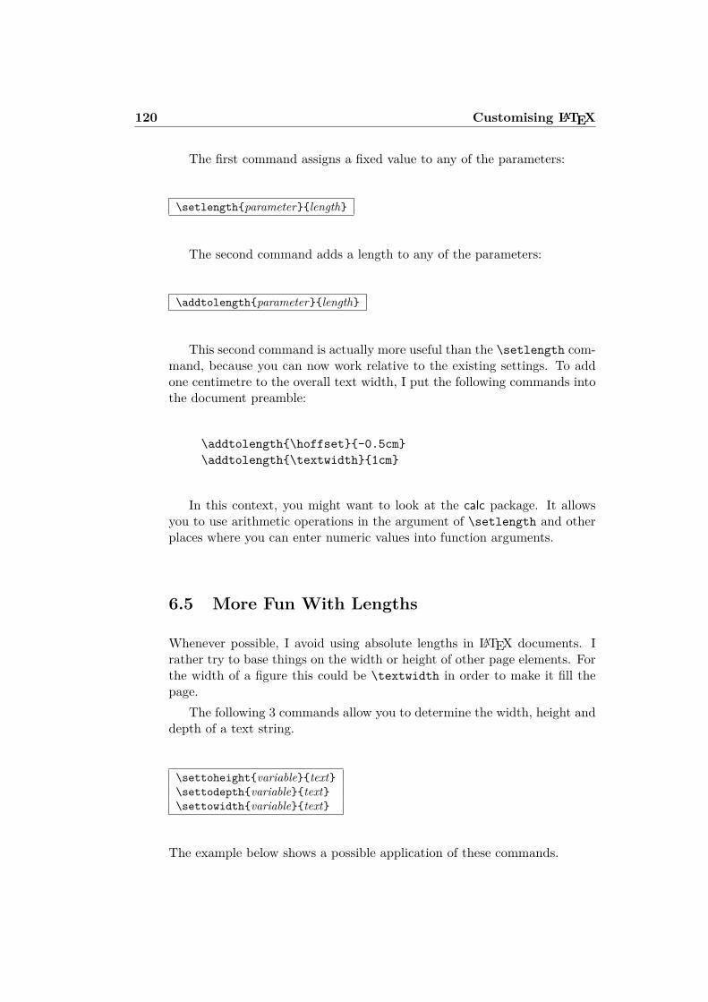
120 Customising LATEX

The first command assigns a fixed value to any of the parameters:

\setlengthparameterlength

The second command adds a length to any of the parameters:

\addtolengthparameterlength

This second command is actually more useful than the \setlength com-mand, because you can now work relative to the existing settings. To addone centimetre to the overall text width, I put the following commands intothe document preamble:

\addtolength\hoffset-0.5cm\addtolength\textwidth1cm

In this context, you might want to look at the calc package. It allowsyou to use arithmetic operations in the argument of \setlength and otherplaces where you can enter numeric values into function arguments.

6.5 More Fun With Lengths

Whenever possible, I avoid using absolute lengths in LATEX documents. Irather try to base things on the width or height of other page elements. Forthe width of a figure this could be \textwidth in order to make it fill thepage.

The following 3 commands allow you to determine the width, height anddepth of a text string.

\settoheightvariabletext\settodepthvariabletext\settowidthvariabletext

The example below shows a possible application of these commands.

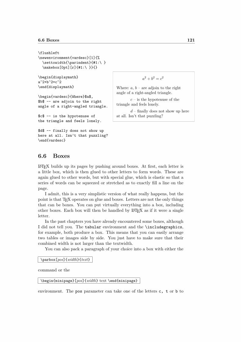
6.6 Boxes 121

\flushleft\newenvironmentvardesc[1]%\settowidth\parindent#1:\ \makebox[0pt][r]#1:\

\begindisplaymatha^2+b^2=c^2\enddisplaymath

\beginvardescWhere$a$,$b$ -- are adjoin to the rightangle of a right-angled triangle.

$c$ -- is the hypotenuse ofthe triangle and feels lonely.

$d$ -- finally does not show uphere at all. Isn’t that puzzling?\endvardesc

a2 + b2 = c2

Where: a, b – are adjoin to the rightangle of a right-angled triangle.

c – is the hypotenuse of thetriangle and feels lonely.

d – finally does not show up hereat all. Isn’t that puzzling?

6.6 BoxesLATEX builds up its pages by pushing around boxes. At first, each letter isa little box, which is then glued to other letters to form words. These areagain glued to other words, but with special glue, which is elastic so that aseries of words can be squeezed or stretched as to exactly fill a line on thepage.

I admit, this is a very simplistic version of what really happens, but thepoint is that TEX operates on glue and boxes. Letters are not the only thingsthat can be boxes. You can put virtually everything into a box, includingother boxes. Each box will then be handled by LATEX as if it were a singleletter.

In the past chapters you have already encountered some boxes, althoughI did not tell you. The tabular environment and the \includegraphics,for example, both produce a box. This means that you can easily arrangetwo tables or images side by side. You just have to make sure that theircombined width is not larger than the textwidth.

You can also pack a paragraph of your choice into a box with either the

\parbox[pos]widthtext

command or the

\beginminipage[pos]width text \endminipage

environment. The pos parameter can take one of the letters c, t or b to

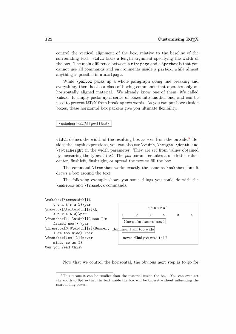
122 Customising LATEX

control the vertical alignment of the box, relative to the baseline of thesurrounding text. width takes a length argument specifying the width ofthe box. The main difference between a minipage and a \parbox is that youcannot use all commands and environments inside a parbox, while almostanything is possible in a minipage.

While \parbox packs up a whole paragraph doing line breaking andeverything, there is also a class of boxing commands that operates only onhorizontally aligned material. We already know one of them; it’s called\mbox. It simply packs up a series of boxes into another one, and can beused to prevent LATEX from breaking two words. As you can put boxes insideboxes, these horizontal box packers give you ultimate flexibility.

\makebox[width][pos]text

width defines the width of the resulting box as seen from the outside.5 Be-sides the length expressions, you can also use \width, \height, \depth, and\totalheight in the width parameter. They are set from values obtainedby measuring the typeset text. The pos parameter takes a one letter value:center, flushleft, flushright, or spread the text to fill the box.

The command \framebox works exactly the same as \makebox, but itdraws a box around the text.

The following example shows you some things you could do with the\makebox and \framebox commands.

\makebox[\textwidth]%c e n t r a l\par

\makebox[\textwidth][s]%s p r e a d\par

\framebox[1.1\width]Guess I’mframed now! \par

\framebox[0.8\width][r]Bummer,I am too wide \par

\framebox[1cm][l]nevermind, so am I

Can you read this?

c e n t r a ls p r e a d

Guess I’m framed now!

Bummer, I am too wide

never mind, so am ICan you read this?

Now that we control the horizontal, the obvious next step is to go for

5This means it can be smaller than the material inside the box. You can even setthe width to 0pt so that the text inside the box will be typeset without influencing thesurrounding boxes.

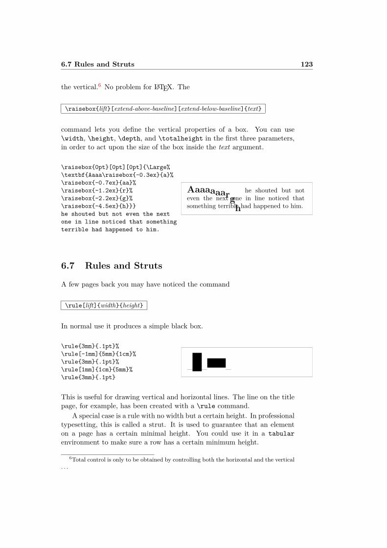
6.7 Rules and Struts 123

the vertical.6 No problem for LATEX. The

\raiseboxlift[extend-above-baseline][extend-below-baseline]text

command lets you define the vertical properties of a box. You can use\width, \height, \depth, and \totalheight in the first three parameters,in order to act upon the size of the box inside the text argument.

\raisebox0pt[0pt][0pt]\Large%\textbfAaaa\raisebox-0.3exa%\raisebox-0.7exaa%\raisebox-1.2exr%\raisebox-2.2exg%\raisebox-4.5exhhe shouted but not even the nextone in line noticed that somethingterrible had happened to him.

Aaaaaaargh

he shouted but noteven the next one in line noticed thatsomething terrible had happened to him.

6.7 Rules and Struts

A few pages back you may have noticed the command

\rule[lift]widthheight

In normal use it produces a simple black box.

\rule3mm.1pt%\rule[-1mm]5mm1cm%\rule3mm.1pt%\rule[1mm]1cm5mm%\rule3mm.1pt

This is useful for drawing vertical and horizontal lines. The line on the titlepage, for example, has been created with a \rule command.

A special case is a rule with no width but a certain height. In professionaltypesetting, this is called a strut. It is used to guarantee that an elementon a page has a certain minimal height. You could use it in a tabularenvironment to make sure a row has a certain minimum height.

6Total control is only to be obtained by controlling both the horizontal and the vertical. . .

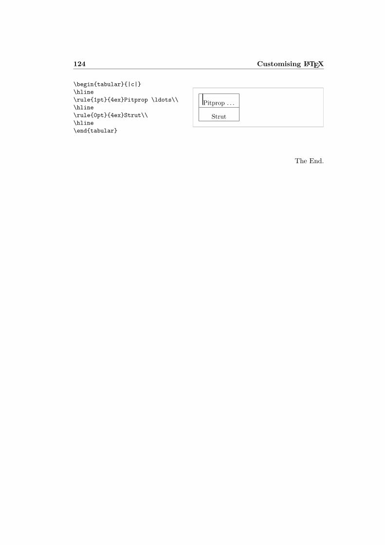
124 Customising LATEX

\begintabular|c|\hline\rule1pt4exPitprop \ldots\\\hline\rule0pt4exStrut\\\hline\endtabular

Pitprop . . .

Strut

The End.

Bibliography

[1] Leslie Lamport. LATEX: A Document Preparation System. Addison-Wesley, Reading, Massachusetts, second edition, 1994, ISBN 0-201-52983-1.

[2] Donald E. Knuth. The TEXbook, Volume A of Computers and Type-setting, Addison-Wesley, Reading, Massachusetts, second edition, 1984,ISBN 0-201-13448-9.

[3] Frank Mittelbach, Michel Goossens, Johannes Braams, David Carlisle,Chris Rowley. The LATEX Companion, (2nd Edition). Addison-Wesley,Reading, Massachusetts, 2004, ISBN 0-201-36299-6.

[4] Michel Goossens, Sebastian Rahtz and Frank Mittelbach. The LATEXGraphics Companion. Addison-Wesley, Reading, Massachusetts, 1997,ISBN 0-201-85469-4.

[5] Each LATEX installation should provide a so-called LATEX Local Guide,which explains the things that are special to the local system. It shouldbe contained in a file called local.tex. Unfortunately, some lazy sysopsdo not provide such a document. In this case, go and ask your localLATEX guru for help.

[6] LATEX3 Project Team. LATEX2ε for authors. Comes with the LATEX2εdistribution as usrguide.tex.

[7] LATEX3 Project Team. LATEX2ε for Class and Package writers. Comeswith the LATEX2ε distribution as clsguide.tex.

[8] LATEX3 Project Team. LATEX2ε Font selection. Comes with the LATEX2εdistribution as fntguide.tex.

[9] D. P. Carlisle. Packages in the ‘graphics’ bundle. Comes with the‘graphics’ bundle as grfguide.tex, available from the same source yourLATEX distribution came from.

[10] Rainer Schöpf, Bernd Raichle, Chris Rowley. A New Implementationof LATEX’s verbatim Environments. Comes with the ‘tools’ bundle as

126 BIBLIOGRAPHY

verbatim.dtx, available from the same source your LATEX distributioncame from.

[11] Vladimir Volovich, Werner Lemberg and LATEX3 Project Team. Cyrilliclanguages support in LATEX. Comes with the LATEX2ε distribution ascyrguide.tex.

[12] Graham Williams. The TeX Catalogue is a very complete listing ofmany TEX and LATEX related packages. Available online from CTAN:/tex-archive/help/Catalogue/catalogue.html

[13] Keith Reckdahl. Using EPS Graphics in LATEX2ε Documents, whichexplains everything and much more than you ever wanted to knowabout EPS files and their use in LATEX documents. Available onlinefrom CTAN:/tex-archive/info/epslatex.ps

[14] Kristoffer H. Rose. XY-pic User’s Guide. Downloadable from CTANwith XY-pic distribution

[15] John D. Hobby. A User’s Manual for METAPOST. Downloadable fromhttp://cm.bell-labs.com/who/hobby/

[16] Alan Hoenig. TEX Unbound. Oxford University Press, 1998, ISBN0-19-509685-1; 0-19-509686-X (pbk.)

[17] Urs Oswald. Graphics in LATEX2ε, containing some Java source filesfor generating arbitrary circles and ellipses within the picture en-vironment, and METAPOST - A Tutorial. Both downloadable fromhttp://www.ursoswald.ch

Index

Symbols\!, 59", 21"’, 34"-, 34"---, 34"<, 34"=, 34">, 34"‘, 34$, 49\,, 51, 58-, 22−, 22\-, 21–, 22—, 22., space after, 34. . . , 23\:, 58\;, 59\@, 34\[, 50\\, 19, 39, 40, 42, 118\\*, 19\], 50~, 34

AA4 paper, 11A5 paper, 11å, 24abstract, 40accent, 24Acrobat Reader, 80acute, 24

\addtolength, 120advantages of LATEX, 3æ, 24aeguill, 81align, 57\Alph, 33\alph, 33\Alpha, 63American Mathematical Society, 49amsbsy, 61amsfonts, 60, 67amsmath, 49, 55–59, 61amssymb, 52, 60, 63amsthm, 61, 62\and, 36ansinew, 26apostrophe, 54\appendix, 35, 36applemac, 26\ar, 103\arccos, 54\arcsin, 54\arctan, 54\arg, 54array, 57, 58arrow symbols, 54article class, 10\Asbuk, 33\asbuk, 33\author, 36, 85

BB5 paper, 11babel, 20, 25, 33, 34\backmatter, 36backslash, 5

128 INDEX

\backslash, 5\bar, 54base font size, 11beamer, 88, 89\begin, 38, 92, 101\Beta, 63\bibitem, 73bibliography, 73\Big, 56\big, 56\Bigg, 56\bigg, 56\bigskip, 118binary relations, 55\binom, 55binomial coefficient, 55blackboard bold, 52block, 90bm, 61Bmatrix, 58bmatrix, 58\bmod, 54bold face, 112bold symbols, 52, 60\boldmath, 61\boldsymbol, 61book class, 10brace

horizontal, 53braces, 56brazilian, 27

Ccalc, 120\caption, 45, 46cases, 58\cdot, 53\cdots, 53center, 39\chapter, 35\chaptermark, 76\ci, 107\circle, 96\circle*, 96

\cite, 73CJK package, 30\cleardoublepage, 46\clearpage, 46\cline, 42color, 88coloured text, 10comma, 23commands, 5

\!, 59\,, 51, 58\-, 21\:, 58\;, 59\@, 34\[, 50\\, 19, 39, 40, 42, 118\\*, 19\], 50\addtolength, 120\Alph, 33\alph, 33\Alpha, 63\and, 36\appendix, 35, 36\ar, 103\arccos, 54\arcsin, 54\arctan, 54\arg, 54\Asbuk, 33\asbuk, 33\author, 36, 85\backmatter, 36\backslash, 5\bar, 54\begin, 38, 92, 101\Beta, 63\bibitem, 73\Big, 56\big, 56\Bigg, 56\bigg, 56\bigskip, 118

INDEX 129

\binom, 55\bmod, 54\boldmath, 61\boldsymbol, 61\caption, 45, 46\cdot, 53\cdots, 53\chapter, 35\chaptermark, 76\ci, 107\circle, 96\circle*, 96\cite, 73\cleardoublepage, 46\clearpage, 46\cline, 42\cos, 54\cosh, 54\cot, 54\coth, 54\csc, 54\date, 36\ddots, 53\DeclareMathOperator, 54\deg, 54\depth, 122, 123\det, 54\dfrac, 55\dim, 54\displaystyle, 60\documentclass, 9, 14, 20\dq, 29\dum, 107\emph, 38, 112\end, 38, 92\enumBul, 33\enumEng, 33\enumLat, 33\eqref, 50\exp, 54\fbox, 21\flq, 29\flqq, 29\foldera, 100

\folderb, 100\footnote, 37, 46\footskip, 119\frac, 55\framebox, 122\frenchspacing, 33, 34\frontmatter, 36\frq, 29\frqq, 29\fussy, 20\gcd, 54\hat, 53\headheight, 119\headsep, 119\height, 122, 123\hline, 42\hom, 54\href, 85, 88\hspace, 109, 116\hyphenation, 20\idotsint, 59\ifpdf, 87\ignorespaces, 109, 110\ignorespacesafterend, 110\iiiint, 59\iiint, 59\iint, 59\include, 14, 15\includegraphics, 72, 83, 87,

121\includeonly, 15\indent, 116\index, 75, 76\inf, 54\input, 15\int, 55\item, 39\ker, 54\label, 37, 46, 50\LaTeX, 21\LaTeXe, 21\ldots, 23, 53\left, 56\leftmark, 76

130 INDEX

\lg, 54\lim, 54\liminf, 54\limsup, 54\line, 94, 100\linebreak, 19\linespread, 115\linethickness, 97, 98, 100\listoffigures, 45\listoftables, 45\ln, 54\log, 54\mainmatter, 36, 86\makebox, 122\makeindex, 75\maketitle, 36\marginparpush, 119\marginparsep, 119\marginparwidth, 119\mathbb, 52\max, 54\mbox, 21, 24, 122\min, 54\multicolumn, 43\multiput, 93, 97\newcommand, 59, 108, 109\newenvironment, 109\newline, 19\newpage, 19\newsavebox, 99\newtheorem, 61\noindent, 116\nolinebreak, 19\nonumber, 57\nopagebreak, 19\not, 64\oddsidemargin, 119\oval, 98, 100\overbrace, 53\overleftarrow, 54\overline, 53\overrightarrow, 54\pagebreak, 19\pageref, 37, 79

\pagestyle, 13\paperheight, 119\paperwidth, 119\par, 112\paragraph, 35\parbox, 121, 122\parindent, 115\parskip, 115\part, 35\partial, 55\phantom, 46, 59\pmod, 54\Pr, 54\printindex, 76\prod, 55\protect, 46\providecommand, 109\ProvidesPackage, 111\put, 93–99\qbezier, 91, 93, 100\qedhere, 62\qquad, 51, 59\quad, 51, 59\raisebox, 123\ref, 37, 46, 79\renewcommand, 108\renewenvironment, 109\right, 56, 58\right., 56\rightmark, 76\rule, 109, 123\savebox, 99\scriptscriptstyle, 60\scriptstyle, 60\sec, 54\section, 35, 46\sectionmark, 76\selectlanguage, 25\setlength, 92, 115, 120\settodepth, 120\settoheight, 120\settowidth, 120\sin, 54\sinh, 54

INDEX 131

\sloppy, 20\smallskip, 118\smash, 51\sqrt, 53\stackrel, 55\stretch, 109, 117\subparagraph, 35\subsection, 35\subsectionmark, 76\substack, 56\subsubsection, 35\sum, 55\sup, 54\tableofcontents, 35\tag, 50\tan, 54\tanh, 54\TeX, 21\texorpdfstring, 86, 87\textcelsius, 22\texteuro, 23\textheight, 119\textstyle, 60\textwidth, 119\tfrac, 55\theoremstyle, 61\thicklines, 95, 98, 100\thinlines, 98, 100\thispagestyle, 13\title, 36\tnss, 108\today, 21\topmargin, 119\totalheight, 122, 123\ud, 59\underbrace, 53\underline, 38, 53\unitlength, 92, 94\usebox, 99\usepackage, 10, 13, 23, 25, 26,

111\vdots, 53\vec, 54\vector, 95

\verb, 41\verbatiminput, 78\vspace, 117\widehat, 53\widetilde, 53\width, 122, 123\xymatrix, 103

comment, 6comments, 6\cos, 54\cosh, 54\cot, 54\coth, 54cp1251, 26cp850, 26cp866nav, 26cross-references, 37\csc, 54curly braces, 5, 112

Ddash, 22\date, 36dcolumn, 43\ddots, 53decimal alignment, 43\DeclareMathOperator, 54\deg, 54degree symbol, 22delimiters, 56\depth, 122, 123description, 39\det, 54Deutsch, 29\dfrac, 55diagonal dots, 53\dim, 54dimensions, 116display style, 49, 51displaymath, 50\displaystyle, 60doc, 12document font size, 11document title, 11

132 INDEX

\documentclass, 9, 14, 20dot, 53dotless ı and , 24dots, 53

three, 53double line spacing, 115double sided, 11\dq, 29\dum, 107

Eeepic, 91, 96ellipsis, 23em-dash, 22\emph, 38, 112empty, 13en-dash, 22Encapsulated PostScript, 71, 83encodings

fontLGR, 27OT1, 26T1, 27, 33T2*, 33T2A, 27, 33T2B, 27T2C, 27X2, 27

inputansinew, 26applemac, 26cp1251, 26cp850, 26cp866nav, 26koi8-ru, 26, 33latin1, 26macukr, 26utf8x, 26

\end, 38, 92\enumBul, 33\enumEng, 33enumerate, 39\enumLat, 33environments

Bmatrix, 58Vmatrix, 58abstract, 40align, 57array, 57, 58block, 90bmatrix, 58cases, 58center, 39comment, 6description, 39displaymath, 50enumerate, 39eqnarray, 57equation*, 50equation, 50figure, 44, 45flushleft, 39flushright, 39frame, 90itemize, 39lscommand, 107matrix, 58minipage, 121, 122parbox, 122picture, 91, 92, 96, 97pmatrix, 58proof, 62pspicture, 92quotation, 40quote, 40table, 44, 45tabular, 41, 121thebibliography, 73verbatim, 41, 78verse, 40vmatrix, 58

epic, 91eqnarray, 57\eqref, 50equation, 49

LATEX, 50amsmath, 50multiple, 57

INDEX 133

equation, 50equation system, 57equation*, 50eurosym, 23executive paper, 11\exp, 54exponent, 52exscale, 12extension, 13

.aux, 14

.cls, 14

.dtx, 13

.dvi, 14, 72

.eps, 72

.fd, 14

.idx, 14, 75

.ilg, 14

.ind, 14, 76

.ins, 14

.lof, 14

.log, 14

.lot, 14

.sty, 13, 78

.tex, 8, 13

.toc, 14

Ffancyhdr, 76–78\fbox, 21figure, 44, 45file types, 13floating bodies, 44\flq, 29\flqq, 29flushleft, 39flushright, 39foiltex, 10\foldera, 100\folderb, 100font, 111

\footnotesize, 112\Huge, 112\huge, 112\LARGE, 112

\Large, 112\large, 112\mathbf, 113\mathcal, 113\mathit, 113\mathnormal, 113\mathrm, 113\mathsf, 113\mathtt, 113\normalsize, 112\scriptsize, 112\small, 112\textbf, 112\textit, 112\textmd, 112\textnormal, 112\textrm, 112\textsc, 112\textsf, 112\textsl, 112\texttt, 112\textup, 112\tiny, 112

font encoding, 12font encodings, 26

LGR, 27OT1, 26T1, 27, 33T2*, 33T2A, 27, 33T2B, 27T2C, 27X2, 27

font size, 111, 112fontenc, 12, 26, 33footer, 13\footnote, 37, 46\footnotesize, 112\footskip, 119formulae, 49\frac, 55fraction, 55fragile commands, 46frame, 90

134 INDEX

\framebox, 122French, 28\frenchspacing, 33, 34\frontmatter, 36\frq, 29\frqq, 29\fussy, 20

G\gcd, 54geometry, 78German, 25, 29GhostScript, 71graphics, 10, 71graphicx, 71, 83, 88grave, 24Greek, 32Greek letters, 52grouping, 112

HHLATEX, 30hLATEXp, 30\hat, 53header, 13\headheight, 119textttheadings, 13\headsep, 119\height, 122, 123\hline, 42\hom, 54horizontal

brace, 53dots, 53line, 53space, 116

\href, 85, 88\hspace, 109, 116\Huge, 112\huge, 112hyperref, 80, 83, 87, 88hypertext, 79hyphen, 22hyphenat, 78

\hyphenation, 20

I\idotsint, 59ifpdf, 87\ifpdf, 87ifthen, 12\ignorespaces, 109, 110\ignorespacesafterend, 110\iiiint, 59\iiint, 59\iint, 59\include, 14, 15\includegraphics, 72, 83, 87, 121\includeonly, 15\indent, 116indentfirst, 116index, 75\index, 75, 76\inf, 54\input, 15input encodings

ansinew, 26applemac, 26cp1251, 26cp850, 26cp866nav, 26koi8-ru, 26, 33latin1, 26macukr, 26utf8x, 26

input file, 7inputenc, 12, 26, 33\int, 55integral operator, 55international, 25italic, 112\item, 39itemize, 39

K\ker, 54Knuth, Donald E., 1koi8-ru, 26, 33

INDEX 135

Korean, 29Korean font

UHC font, 31Korean input files, 29

L\label, 37, 46, 50Lamport, Leslie, 2language, 25\LARGE, 112\Large, 112\large, 112\LaTeX, 21LATEX3, 4\LaTeXe, 21latexsym, 12latin1, 26layout, 118\ldots, 23, 53\left, 56left aligned, 39\leftmark, 76legal paper, 11letter paper, 11\lg, 54LGR, 27ligature, 24\lim, 54\liminf, 54\limsup, 54line

horizontal, 53\line, 94, 100line break, 19line spacing, 115\linebreak, 19\linespread, 115\linethickness, 97, 98, 100\listoffigures, 45\listoftables, 45\ln, 54\log, 54long equations, 57longtable, 43

lscommand, 107

Mmacukr, 26\mainmatter, 36, 86\makebox, 122makeidx, 12, 75makeidx package, 75\makeindex, 75makeindex program, 75\maketitle, 36\marginparpush, 119\marginparsep, 119\marginparwidth, 119margins, 118math mode, 51math spacing, 58\mathbb, 52\mathbf, 113\mathcal, 113mathematical

accents, 53delimiter, 56functions, 54minus, 22

mathematics, 49\mathit, 113\mathnormal, 113\mathrm, 113mathrsfs, 67\mathsf, 113mathtext, 33\mathtt, 113matrix, 58matrix, 58\max, 54\mbox, 21, 24, 122METAPOST, 83mhchem, 60\min, 54minimal class, 10minipage, 121, 122minus sign, 22Mittelbach, Frank, 2

136 INDEX

mltex, 81mltex, 81modulo function, 54\multicolumn, 43\multiput, 93, 97

N\newcommand, 59, 108, 109\newenvironment, 109\newline, 19\newpage, 19\newsavebox, 99\newtheorem, 61\noindent, 116\nolinebreak, 19\nonumber, 57\nopagebreak, 19\normalsize, 112\not, 64ntheorem, 62

O\oddsidemargin, 119œ, 24one column, 11option, 9optional parameters, 5OT1, 26\oval, 98, 100\overbrace, 53overfull hbox, 20\overleftarrow, 54\overline, 53\overrightarrow, 54

Ppackage, 7, 10, 107packages

aeguill, 81amsbsy, 61amsfonts, 60, 67amsmath, 49, 55–59, 61amssymb, 52, 60, 63amsthm, 61, 62babel, 20, 25, 33, 34

beamer, 88, 89bm, 61calc, 120color, 88dcolumn, 43doc, 12eepic, 91, 96epic, 91eurosym, 23exscale, 12fancyhdr, 76–78fontenc, 12, 26, 33geometry, 78graphicx, 71, 83, 88hyperref, 80, 83, 87, 88hyphenat, 78ifpdf, 87ifthen, 12indentfirst, 116inputenc, 12, 26, 33latexsym, 12layout, 118longtable, 43makeidx, 12, 75mathrsfs, 67mathtext, 33mhchem, 60mltex, 81ntheorem, 62ppower4, 88prosper, 88pstricks, 91, 92, 96pxfonts, 82showidx, 76syntonly, 12, 15textcomp, 22, 23txfonts, 82ucs, 26verbatim, 6, 78xy, 102

page layout, 118page style, 13

empty, 13headings, 13

INDEX 137

plain, 13\pagebreak, 19\pageref, 37, 79\pagestyle, 13paper size, 11, 80, 118\paperheight, 119\paperwidth, 119\par, 112paragraph, 17\paragraph, 35parameter, 5\parbox, 121, 122parbox, 122\parindent, 115\parskip, 115\part, 35\partial, 55partial derivative, 55PDF, 79PDFLATEX, 88pdfLATEX, 81, 88pdfLATEX, 80pdfTEX, 80period, 23\phantom, 46, 59picture, 91, 92, 96, 97piecewise function, 58placement specifier, 45plain, 13pmatrix, 58\pmod, 54Português, 27Portuguese, 27PostScript, 3, 9, 31, 46, 71, 72, 81,

82, 92Encapsulated, 71, 83

ppower4, 88\Pr, 54preamble, 7prime, 54\printindex, 76proc class, 10\prod, 55product operator, 55

proof, 62prosper, 88\protect, 46\providecommand, 109\ProvidesPackage, 111pspicture, 92pstricks, 91, 92, 96\put, 93–99pxfonts, 82

Q\qbezier, 91, 93, 100\qedhere, 62\qquad, 51, 59\quad, 51, 59quotation, 40quotation marks, 21quote, 40

R\raisebox, 123\ref, 37, 46, 79\renewcommand, 108\renewenvironment, 109report class, 10reserved characters, 5\right, 56, 58right-aligned, 39\right., 56\rightmark, 76roman, 112\rule, 109, 123

Ssans serif, 112\savebox, 99Scandinavian letters, 24\scriptscriptstyle, 60\scriptsize, 112\scriptstyle, 60\sec, 54\section, 35, 46\sectionmark, 76\selectlanguage, 25\setlength, 92, 115, 120

138 INDEX

\settodepth, 120\settoheight, 120\settowidth, 120showidx, 76\sin, 54single sided, 11\sinh, 54slanted, 112slides class, 10\sloppy, 20\small, 112Small Caps, 112\smallskip, 118\smash, 51space, 4spacing

math mode, 51special character, 24\sqrt, 53square brackets, 5square root, 53\stackrel, 55\stretch, 109, 117structure, 7strut, 123\subparagraph, 35subscript, 52\subsection, 35\subsectionmark, 76\substack, 56\subsubsection, 35\sum, 55sum operator, 55\sup, 54syntonly, 12, 15

TT1, 27, 33T2*, 33T2A, 27, 33T2B, 27T2C, 27table, 41table, 44, 45

table of contents, 35\tableofcontents, 35tabular, 41, 121\tag, 50\tan, 54\tanh, 54\TeX, 21\texorpdfstring, 86, 87text style, 49, 51\textbf, 112\textcelsius, 22textcomp, 22, 23\texteuro, 23\textheight, 119\textit, 112\textmd, 112\textnormal, 112\textrm, 112\textsc, 112\textsf, 112\textsl, 112\textstyle, 60\texttt, 112\textup, 112\textwidth, 119\tfrac, 55thebibliography, 73\theoremstyle, 61\thicklines, 95, 98, 100\thinlines, 98, 100\thispagestyle, 13tilde, 22, 53tilde ( ~), 34\tiny, 112title, 11, 36\title, 36\tnss, 108\today, 21\topmargin, 119\totalheight, 122, 123two column, 11txfonts, 82

INDEX 139

Uucs, 26\ud, 59umlaut, 24\underbrace, 53underfull hbox, 20\underline, 38, 53\unitlength, 92, 94units, 116, 117upright, 112URL, 22\usebox, 99\usepackage, 10, 13, 23, 25, 26, 111utf8x, 26

V\vdots, 53\vec, 54\vector, 95vectors, 54\verb, 41verbatim, 6, 78verbatim, 41, 78\verbatiminput, 78verse, 40vertical

dots, 53vertical space, 117Vmatrix, 58vmatrix, 58\vspace, 117

Wwhitespace, 4

after commands, 5at the start of a line, 4

\widehat, 53\widetilde, 53\width, 122, 123Word, 76www, 22WYSIWYG, 2, 3

XX2, 27

Xpdf, 80xy, 102\xymatrix, 103