SJP QM 3220 Ch. 2, part 1 Page 1 Once again, the...

SJP QM 3220 Ch. 2, part 1

(S. Pollock, taken from M. Dubson) with thanks to J. Anderson for typesetting. Fall 2008

Once again, the Schrödinger equation:

↑ (which can also be written Ĥ ψ(x,t) if you like.)

And once again, assume V = V(x) (no t in there!) We can start to solve the PDE by SEPARATION OF VARIABLES. Assume (hope? wonder if?) we might find a solution of form Ψ (x,t) = u(x) φ(t). Griffiths calls u(x) ≡ ψ(x), but I can't distinguish a "small ψ" from the "capital Ψ" so easily in my handwriting. You’ll find different authors use both of these notations…)

So Note full derivative on right hand side!

So Schrödinger equation reads (with

€

dφdt

≡ φ•

, and dudx

≡ u' )

Now divide both sides by Ψ = u • φ.

€

i φ(t)•

φ(t)functionoftimeonly

= −2

2mu' '(x)u(x)

+V (x)

functionofspaceonly

This is not possible unless both sides are constants. Convince yourself; that is the key to the "method of separation of variables". Let's name this constant "E".

[Note units of E are or simply V(x), either way, check, it's Energy!]



So (1)

(2) These are ordinary O.D.E.'s

Equation (1) is about as simple as ODE's get! Check

any constant, it's a linear ODE. (1st order linear ODE is supposed to give one undetermined constant, right?) This is "universal", no matter what V(x) is, once we find a u(x), we'll have a corresponding But be careful, that u(x) depends on E,

(2) .

↑ this is This is the "time independent Schrödinger equation". You can also write this as which is an "eigenvalue equation". Ĥ = "Hamiltonian" operator = In general, has many possible solutions.

eigenfunctions eigenvalues u1(x), u2(x), … un(x) may all work, each corresponding to some particular eigenvalue E1, E2, , … En. (What we will find is not any old E is possible if you want u(x) to be normalizable and well behaved. Only certain E's, the En's, will be ok.) Such a un(x) is called a "stationary state of Ĥ". Why? Let’s see…



Notice that Ψn(x,t) corresponding to un is

◄══ go back a page!

So ◄══ no time dependence (for the probability density). It's not evolving in time; it's "stationary". (Because ) Convince yourself! (If you think back to de Broglie's free particle

with E = , it looks like we had stationary states Ψn(x,t) with this (same) simple time dependence, eiωt , with . This will turn out to be quite general)

If you compute

€

ˆ Q (the expectation value of any operator “Q” for a stationary state) the

€

e−iEnt / in Ψ multiplies the

€

eiEnt / in Ψ*, and goes away… (This is assuming the operator Q depends on x or p, but not time explicitly)

again, no time dependence. Stationary state are dull, nothing about them (that's measurable) changes with time. (Hence, they are "stationary"). ──►(Not all states are stationary … just these special states, the Ψn's) And remember, ◄─ Time Indep. Schröd. eq'n (2) and also This is still the Schrödinger Equation! (after plugging in our time solution for φ(t). )

€

ψfree = Aeikxe−iωt

€



Check this out though: for a state Ψn (x,t)

In stationary Ψn

constants come out this is normalization! of integrals So the state Ψn "has energy eigenvalue En" and has expectation value of energy En. and so Think about this – there is zero “uncertainty” in the measurement of H for this state. Conclusion: Ψn is a state with a definite energy En. (no uncertainty!) (that's really why we picked the letter E for this eigenvalue!) Remember, is linear, so … If Ψ1 and Ψ2 are solutions, so is (aΨ1 + bΨ2 .) But, this linear combo is not stationary! It does not have any "energy eigenvalue" associated with it!



The most general solutions of

€

ˆ H Ψn = i ∂Ψ∂t

(given V= V(x)) is thus

. energy eigenstate , or "stationary state" . any constants you like, real or complex, Just so long as you ensure Ψ is normalized. .

If you measure energy on a stationary state, you get En, (definite value), (But if you measure energy on a mixed or general state,…we need to discuss this further! Hang on …)

not an energy eigenstate not stationary It's a "mixed energy!"

Simple time dependence for each term

Any/every physical state can be expressed in this way, as a combination of the more special stationary states, or "eigenstates".



The Infinite Square Well: Let's make a choice for V(x) which is solvable that has some (approximate) physical relevance.

It's like the limit of

Classically,

€

F = −

dVdx

is 0 in the middle (free) but big at the edges. Like walls at the edges.

(Like an electron in a small length of wire:

free to move inside, but stuck, with large force at the ends prevents it from leaving.) Given V(x), we want to find the special stationary states (and then we can construct any physical state by some linear combination of those!)

a

|

V(x)

as this gets big (height)

x

V(x)

0 a x

V(x) = 0 for 0 < x < a = ∞ elsewhere

and this gets small (distance where it rises)



Recall, we're looking for un(x) such that

€

ˆ H un (x) = Enun (x) (and then

€

Ψn (x, t) = un (x)e−iEnt )

(or, dropping "n" for a sec) (and then at last)

€

−2

2mu' '(x) +V (x)u(x) = E ⋅ u(x)

€

Ψgeneral (x, t) = cnn∑ Ψn (x, t)

Inside the well, 0 < x < a, and V(x) = 0, so in that region

€

d2udx 2

= −2mE2 u(x) ≡ −k 2u(x) Here, I simply defined

€

k ≡ 2mE

It's just shorthand,

€

k ≡2mE

so

€

E =2

2mk 2

(However, I have used the fact that E > 0, you can't ever get E < Vmin = 0! Convince yourself!) I know this 2nd order ODE, and its general solution is u(x) = A sin kx + B cos kx or α eikx + β e-ikx But Postulate I says u(x) should be continuous. Now, outside 0 < x < a, V(x) ─►∞. This is unphysical, the particle can't be there! So u(x) = 0 at x = 0 and x = a. This is a BOUNDARY CONDITION. u(x = 0) = A • 0 + B • 1 = 0 so B = 0. (required!) u(x = a) = A • sin ka = 0. But now, I can't set A = 0 'cause then u(x) = 0 and that's not normalized. So sin ka = 0, i.e. k = nπ / a with n = 1, 2, 3, …

Ah ha! The boundary condition forced us to allow only certain k's. Call them

€

kn =nπa

Then since

€

E =2

2mk 2 ,we get

€

En =n2π 22

2ma2

(Note: negative n's just re-define "x", it's not really a different state, A sin (kx) is the same function as A sin (-kx)). (Note: n = 0 no good, because sin (0x) = 0 is not normalizable!)



Thus, our solutions, the "energy eigenstates" are

€

un (x) = Asin(kn x) = Asin nπxa

n= 1, 2, 3, … (0 < x < a)

(and 0 elsewhere)

and

€

En = n2 π 22

2ma2

For normalization,

€

un (x)2dx =1⇒ A 2

⋅∫ sin20

a∫ nπx

adx =1

Convince yourself, then,

€

A 2=2a

is required.

So

€

un (x) =2asin nπx

a

(for 0<x<a)

(Note sign/phase* out front is not physically important. If you multiply un(x) by eiθ, you have a wavefunction with the same |u(x)|2, it's physically indistinguishable. So e.g. un(x) and –un(x) are not "different eigenstates".

Energy is quantized (due to boundary condition on U) Energies grow like n2 Lowest energy is not 0! (You cannot put an electron in a box and have it be at

rest!)

0

E1

4E1

En

n=1

n=2

n=3 These are excited states

This is ground state

Energies are E1, 4E1, 9E1, …

n=2 n=3

etc.

n=1



Key properties to note (many of which will be true for most potentials, not just this one!) Energy eigenstates un(x) are …

"even" or "odd" with respect to center of box (n=1 is even, n=2 is odd, this alternates)

oscillatory, and higher energy ◄═► more nodes or zero crossings. (Here, un has (n-1) intermediate zeros)

orthogonal:

€

un0

a

∫ (x)um (x)dx = δnm =0 if n ≠ m1 if n = m

check this, if you don't know why

€

sin nπxa

forms orthogonal states, work it out.

complete: Dirichlet's Theorem, the basis of "Fourier series" says ANY function f(x) which is 0 at x = 0 and x = a can be written, uniquely,

€

f (x) = cnun (x)n=1

∞

∑ can always find the cn's:

(Recall,

€

un =2asin nπx

a here)

Fourier's trick finds those cn's, given an f(x): If

€

f (x) = cnψ n (x)n∑ then do "the trick" …

Multiply both sides by "psi*",

€

f (x)ψ m* (x) = cnψ n (x)ψ m

* (x)n∑

Then integrate, so

€

f (x)0

a

∫ ψ m* (x)dx = cn ψ n (x)ψ m

* (x)0

a

∫This is δ nm . Here our ψ is real, so * isn' t important in this example

n∑ dx

Note that only ONE term, the one with n =m,contributes in this sum. All others vanish!

This tells us (flipping left and right sides)

€

cm = f (x)ψ m* (x)dx

0

a

∫ ◄─ this is how you figure out cm's!

(The above features are quite general! Not just this problem!)



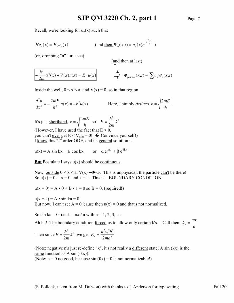
And last but not least, this was all for un(x), but the full time-dependent stationary states

are

€

un (x)e−iEnt , or writing it out:

€

Ψn (x, t) =

2asin nπx

a

e−in 2π 2 2 / 2ma 2

t

this particular functional form is specific to "particle in box" This is still a stationary state, full solution to "Schröd in a box" with definite energy En. These are special, particular states, "eigenstates of Ĥ". The most general possible state of any "electron in a 1-D box", then, would be any linear combo of these:

€

ψ (x, t) = cnΨn (x, t)n∑ = cnun (x)e

−iEnt /

n∑

You can pick any cn's you like (even complex!) and this will give you all possible physical states. You might choose the cn's to give a particular Ψ(x,t=0) that you start with, using Fourier's trick! If

€

Ψ(x,0) = cnunn∑ is given, find the cn's,

and then the formula at top of page tells you Ψ(x,t). [So given initial conditions, we know the state at all times. That's the goal of physics!] For other potentials, game is same: find un(x)'s and corresponding En's, then form a linear combo at t=0 to match your starting state, and let it evolve,

€

ψ (x, t) = cnun (x)e−iEnt /

n∑ …



One last comment: If

€

ψ(x, t) = cnun (x)e−iEnt /

n∑

then normalization says

€

Ψ*Ψdx =1∫ But when you expand Ψ* and Ψ, all cross terms vanish after integration,

€

un* (x)um∫ (x)dx = δnm , leaving only the terms with n=m, which integrate simply.

Work it out:

€

Ψ*Ψdx =1∫ tells you

€

1=m∑

n∑ cm

* cn um* (x)un (x)

ei(Em −En )t / dx∫

Note: this collapses the whole integral to δmn, (thus ei(stuff)… ─►1)

€

= cm* cnδmn

mn∑

€

= cn2

n∑ ◄── convince yourself.

Similarly (try it!) use Ĥψn = Enψn, to get

€

H = Ψ* ˆ H Ψ = En cnn∑∫

2

Interpretation (which we'll develop more formally)

€

ψ (x, t) = cnun (x)e−iEnt /

n∑ = cnΨn (x, t)

n∑

says "the state Ψ is a linear combination of the special stationary states, the Ψn's." The cn's carry information,

€

H = cnn∑

2En which looks like

€

Pnn∑ En

|cn|2 = Probability that this particle's energy would be measured En. (so

€

cnn∑

2= 1 is just "conservation of probability".)

This is a central concept in QM, we'll come back to it often.



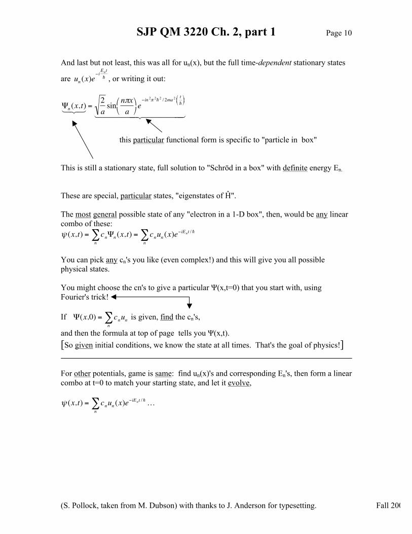
The Harmonic Oscillator: Many objects experience a (classical) force F = -k x , Hooke's Law. This is the harmonic oscillator, and V(x) = ½ k x2. Note that almost any V(x) with a minimum will look at least approximately like this, at least for small x, so it's physically a very common situation! Classically, x(t) = A sin ωt + B cos ωt for Harm. Osc. with ω ≡√k/m (so V = ½ m ω 2 x2 ) ↑ a defined quantity, but it tells you period T = 2π / ω. So let's consider the Quantum Harmonic Oscillator. As before, separate x and t, and look for solutions not 0.

€

−

2

2mu' '(x) +

12mω 2x 2u(x) = E u(x) these u's will give us stationary states.

(then, if you find such a u,

€

ψ (x, t) = u(x)e−iEt / gives the time dependence.) Just like before, we will find that, if we insist

€

u(x)→x→∞

0 , (i.e. our "boundary cond."), then we will find only certain E's, called En, will, and the corresponding un(x) will be unique. So just like in the box, we'll have Ψn(x,t)'s, each n corresponding to a stationary state with discrete energy. This differential equation is a 2nd order ODE but that "x2" term makes it hard to solve. There are tricks. (*See aside, next page) Trick #1: For large x, x2 dominates, so

€

−

2

2mu' '(x) = (E - 1

2mω 2x 2)u ≈

largex

- 12mω 2x 2u

Solution (check, it's not familiar)

€

u(x) = Ae−mωx 2

2 2 + Be+mωx 2

2 2 (Note: 2 undetermined constants for 2nd order ODE, nice!) (↑ This B term is very nasty as x → ∞, toss is as unphysical! Next comes trick #1 part 2, which is to "factor out" this large x behavior:



Let's now assume (hope, wonder if?)

€

u(x) = h(x)e−mω2x 2 / 2 2 , and hope that maybe h(x)

will be "simple". Indeed, use the (love this name!) Method of Frobenius: try h(x) =? a0 + a1x + a2x2 + … Plug in, see what happens… For now, I'm going to skip this algebraically tedious exercise and skip to the punchline: If you insist that u(x) stays normalizable, you find that series for h(x) needs to end, it must be a finite order polynomial. And that will happen if and only if E takes on special

values, namely

€

En = n +12

ω (where "n" is an integer)

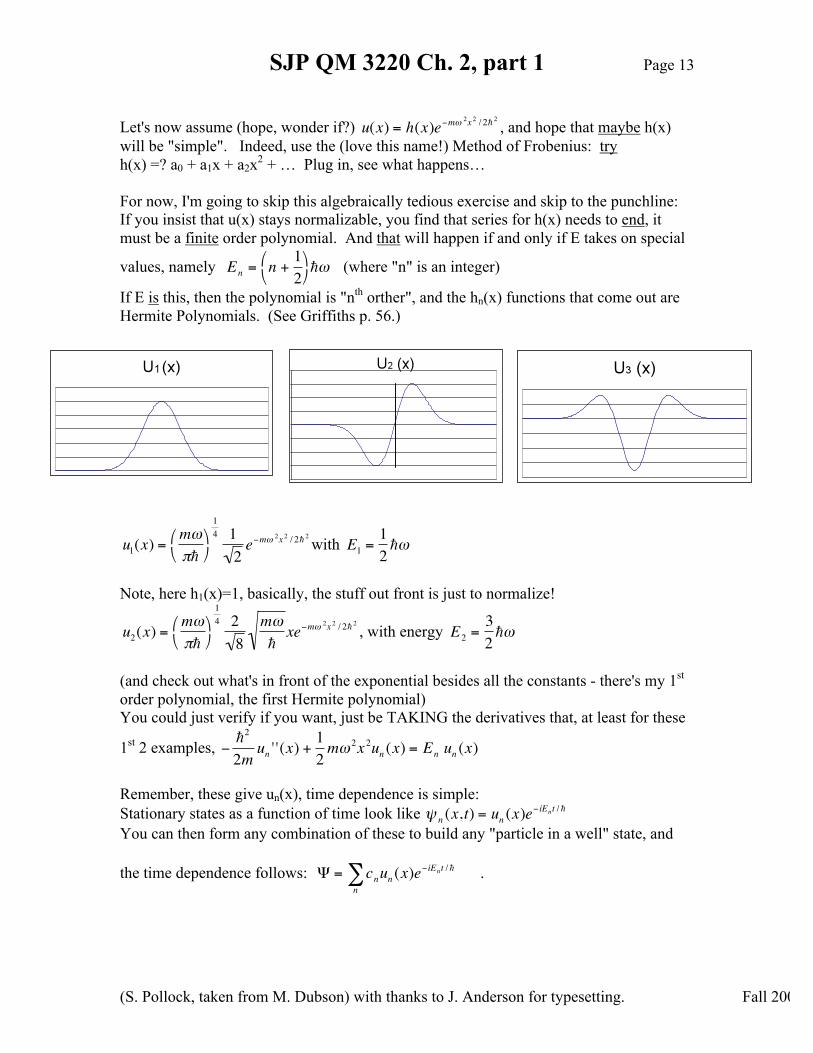
If E is this, then the polynomial is "nth orther", and the hn(x) functions that come out are Hermite Polynomials. (See Griffiths p. 56.)

€

u1(x) =mωπ

14 12e−mω

2x 2 / 2 2 with

€

E1 =12ω

Note, here h1(x)=1, basically, the stuff out front is just to normalize!

€

u2(x) =mωπ

14 28

mωxe−mω

2x 2 / 2 2 , with energy

€

E2 =32ω

(and check out what's in front of the exponential besides all the constants - there's my 1st order polynomial, the first Hermite polynomial) You could just verify if you want, just be TAKING the derivatives that, at least for these

1st 2 examples,

€

−

2

2mun ' '(x) +

12mω 2x 2un (x) = En un (x)

Remember, these give un(x), time dependence is simple: Stationary states as a function of time look like

€

ψ n (x,t) = un (x)e− iEnt /

You can then form any combination of these to build any "particle in a well" state, and the time dependence follows:

€

Ψ = cnn∑ un (x)e

−iEnt / .



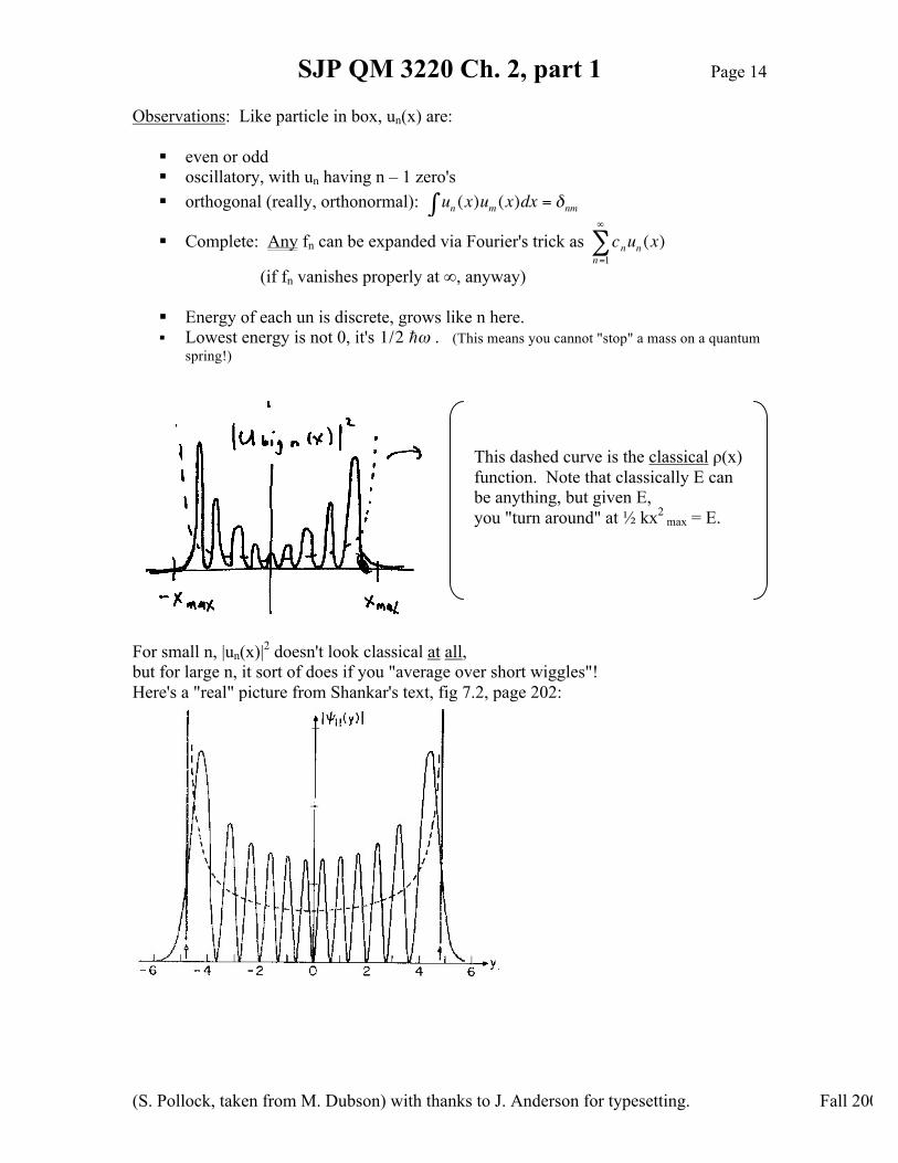
Observations: Like particle in box, un(x) are:

even or odd oscillatory, with un having n – 1 zero's orthogonal (really, orthonormal):

€

un (x)um∫ (x)dx = δnm

Complete: Any fn can be expanded via Fourier's trick as

€

cnn=1

∞

∑ un (x)

(if fn vanishes properly at ∞, anyway)

Energy of each un is discrete, grows like n here. Lowest energy is not 0, it's

€

1/2 ω . (This means you cannot "stop" a mass on a quantum spring!)

For small n, |un(x)|2 doesn't look classical at all, but for large n, it sort of does if you "average over short wiggles"! Here's a "real" picture from Shankar's text, fig 7.2, page 202:

This dashed curve is the classical ρ(x) function. Note that classically E can be anything, but given E, you "turn around" at ½ kx2

max = E.



--- AnAside --- Another method to know of, you might call it Trick #2: Numerical solutions!

How to solve

€

u' '= − 2m

2 (E -V(x))u(x) ? (without yet knowing E!)

Even solutions: Guess an E (use a similar situation, or just units? For Harmonic Oscillator,

€

ω has units of energy, so maybe just try it as a starting guess, call it

€

˜ E .) Let u(0) = 1, u'(0) = 0 ◄─ flat at origin, since I'm looking for the even solution! u(0) may not be 1, but we'll normalize later! Now, pick a "step-size" ε (tiny!) We'll "step along" in x, finding u(x) point by point…

Use S.E. to tell you u''(0).

€

u' '(0) = −2m

2 ( ˜ E - V(0))u(0)

Use u'(0) = u(ε) – u(0) to compute u(ε) ε

Use u''(0) = u'(ε) – u'(0) to compute u'(ε) ε Now repeat, stepping across x in stops of ε. If u starts to blow up, you need more curvature at start, so raise

€

˜ E and start again. If u blows down you need less curvature, lower

€

˜ E For odd solutions, start with u(0) = 0, u'(0) = 1 (again, u'(0) may not be 1, but we'll renormalize later) Otherwise, it's the same game … So basically you pick an E, numerically "shoot" from the origin, and keep fixing E till you get a solution which behaves well at large x. In this way, you can plot/compute u(x) and find the energies, for essentially any V(x). (In this sense, you don't have to feel bad that only a few V(x)'s yield analytic solutions for un(x) and En. All V's can be "solved" numerically.)

--- EndAside ---



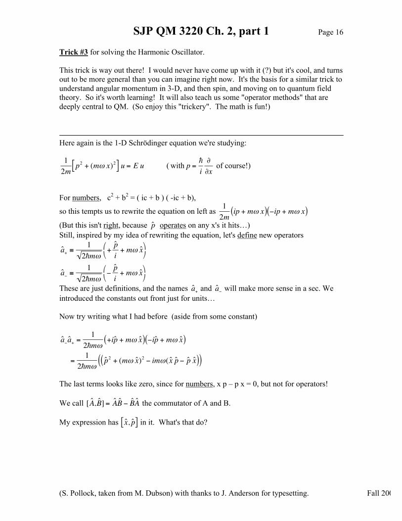
Trick #3 for solving the Harmonic Oscillator. This trick is way out there! I would never have come up with it (?) but it's cool, and turns out to be more general than you can imagine right now. It's the basis for a similar trick to understand angular momentum in 3-D, and then spin, and moving on to quantum field theory. So it's worth learning! It will also teach us some "operator methods" that are deeply central to QM. (So enjoy this "trickery". The math is fun!) Here again is the 1-D Schrödinger equation we're studying:

€

12m

p2 + (mω x)2[ ] u = E u (

€

with p =

i∂∂x

of course!)

For numbers, c2 + b2 = ( ic + b ) ( -ic + b),

so this tempts us to rewrite the equation on left as

€

12m

ip + mω x( ) −ip + mω x( )

(But this isn't right, because

€

ˆ p operates on any x's it hits…) Still, inspired by my idea of rewriting the equation, let's define new operators

€

ˆ a + ≡1

2mω+

ˆ p i

+ mω ˆ x

ˆ a − ≡1

2mω−

ˆ p i

+ mω ˆ x

These are just definitions, and the names

€

ˆ a + and

€

ˆ a − will make more sense in a sec. We introduced the constants out front just for units… Now try writing what I had before (aside from some constant)

€

ˆ a − ˆ a + =1

2mω+iˆ p + mω ˆ x ( ) −iˆ p + mω ˆ x ( )

=1

2mωˆ p 2 + (mω ˆ x )2 − imω( ˆ x ˆ p − ˆ p ˆ x ( )( )

The last terms looks like zero, since for numbers, x p – p x = 0, but not for operators! We call

€

[ ˆ A , ˆ B ] = ˆ A ̂ B − ˆ B ̂ A the commutator of A and B. My expression has

€

ˆ x , ˆ p [ ] in it. What's that do?



What does

€

ˆ x , ˆ p [ ] mean? It's an operator, so consider acting it on any old function f(x) :

€

ˆ x , ˆ p [ ] f (x) = ( ˆ x ̂ p − ˆ p ̂ x ) f = x

i∂∂x

f −

i∂∂x

this operateson (xf )!

x f

but

€

∂∂x(xf ) = f + x

∂f∂x

. The term

€

x∂f∂x

explicitly cancels, leaving

(please check this for yourself)

€

ˆ x , ˆ p [ ] f = −

if .

Since f(x) is totally arbitrary, this is try for ANY f, we say

€

ˆ x , ˆ p [ ] = −

i

This is very important,

€

ˆ x , ˆ p [ ] = i , it's not zero! (we'll talk much more about this!) OK, back to our problem: looking again at that product of

€

ˆ a − and

€

ˆ a + , we have

€

ˆ a − ˆ a + =1

2mω( ˆ p 2 + (mω ˆ x )2) − imω

2mω⋅ (i)

=1ω

ˆ H +12

or ˆ H = ω( ˆ a − ˆ a + −12

)

Now go through yourself and convince yourself that if instead we had written down that product in the opposite order, we would have gotten

€

ˆ H = ω( ˆ a + ˆ a −oppositeorder

+

12

) (note the other sign for the 1/2 term at the end)

And indeed, we can easily compute the commutor of

€

ˆ a − and

€

ˆ a + (which you could do directly by writing out

€

ˆ a − and

€

ˆ a + in detail, but it's easier to use the expressions just above):

€

ˆ a −, ˆ a +[ ] =1ω

ˆ H +12

−

1ω

ˆ H −12

= 1

OK, but why have we done all this?? Here comes the crux (#1 ) . . . Suppose u(x) is a solution to Ĥ u = E u i.e. suppose we knew the u's ( which is what we're after, remember!) Let's consider acting H on

€

ˆ a + which in turn is acting on u. (Why? You'll see!)



€

ˆ H ( ˆ a +u) = ω( ˆ a + ˆ a − +12

)

This is just ˆ H

( ˆ a +u)

= ω( ˆ a + ˆ a − ˆ a + +12

ˆ a +)u

= ωˆ a +( ˆ a − ˆ a + +12

)u

€

= ˆ a +ωConstants slide past a + , right?

( ˆ a + ˆ a − +1

Here I used [a - , a + ]=1So a -a + -a +a - = 1

+

12

)u

= ˆ a +(ω ( ˆ a + ˆ a − +12

)

But, this is just ˆ H again!

+ ω u

Look over all the steps, these tricks are not hard, but require some practice. This is "operator methods", we'll play this sort of game more often later in the course! OK, one more step: now use Ĥ u = Eu Thus

€

ˆ H ( ˆ a +u) = ˆ a +(E + ω) u or

€

ˆ H ( ˆ a +u) = (E + ω) (ˆ a +u) So

€

(ˆ a +u) is an eigenfunction of H with eigenvalue

€

(E + ω) Given u, I found a new, different eigenfunction with a different eigenvalue. Now you try it, this time with Ĥ ( â- u ). I claim you'll get

€

(E − ω) ( ˆ a −u) . So now we see the use of â+ or â-: they generate new solutions, different eigenvalues and eigenfunctions. â+ = "raising operator" because it raises E by

€

ω . â- = "lowering operator" because it lowers E by

€

ω . They are "ladder operators" because E changes in steps of

€

ω .



Now for crux #2 … If you apply

€

ˆ a − ˆ a − ˆ a −… ˆ a −m of these

u you create a state with

€

E − mω .

You can always pile up enough a-'s to get a negative energy… but there's a theorem that says E can never be lower than the minimum of V(x), which is 0. ACK! This is bad … unless there is a bottom state u0, such that a- u0 = 0. (That's the ONLY way out! If there was no such "bottom state", then we could always find a physical state which is impossible - one with negative energy) Note that 0 "solves" the S. Eq., it's just not interesting. And from then on applying more â-'s doesn't cause any new troubles:

€

ˆ a − ˆ a −u0 = ˆ a −0 = 0… OK, so

€

ˆ a −u0(x) = 0 . Let's write this equation out in detail, because we know what â- is:

€

12mω

ddx

+ mω x

u0 = 0

That's no problem to solve! See Griffiths, or just check for yourself:

€

u0(x) = Ae−mωx2 / 2works (for any x) And it's a 1st order ODE, so with one unedtermined

coefficient (A) here, that's the most general solution.

We can even find A: pick it to normalize u0(x) (use the handy relation

€

e−x2

dx = π−∞

∞

∫ )

So

€

u0(x) =mωπ

14e−mωx

2 / 2 .

This solves S.E., just plug it in! On the right, you'll see E0 pop out,

€

E0 =12ω.

Indeed, there's a very cute operator trick to see this directly:

€

ˆ H u0 = E0u0 ⇒ ω( ˆ a + ˆ a −this "kills" u0

+1/2)u0 = E0u0

so 12ω u0 = E0u0

_________



OK, we found the "bottom of the ladder". But now, â+ u0 gives another state, (call it u1),

with

€

E1 = E0 + ω =32ω. (although, you may have to normalize again!)

And in general, climbing back up the ladder,

€

un (x) = An ( ˆ a +)n u0(x) with En = (n +12

)ω

(Although you must normalize each one separately - see Griffiths or homework!) ______ Question: could we have missed some solutions in this way? Might there be a

€

˜ u (x) which is not "discovered" by repeated applications of â+ to u0? Fortunately no. If there were,

€

( ˆ a −)n ˜ u (x) would still have to give 0 for some n, and thus there'd be a "lowest"

€

˜ u (x)… but we found the unique lowest state already! Griffiths has a cute trick to normalize the states, see p. 47 - 48. He also has an elegant trick to prove

€

um*

−∞

∞

∫ (x)un (x)dx = δmn (see page 49) But let's leave this for now: Bottom line: By "Frobenius" or "ladder operators", we found all the stationary states

un(x), with

€

En = (n +12)ω.

(In general, potentials V(x) give "bound states", with discrete energies.) But let's move on to a qualitatively different problem, where we're not bound!



The Free Particle: Consider V(x) = 0. No PE, just a free particle. We talked about this at the start, (de Broglie's ideas). Now we can tackle it with the Schrödinger Equation. There is some funny business here, but clearly this too is an important physics case, we need to describe quantum systems that aren't bound!

)()('' xuExum

⋅=−2

2 That looks easy enough!

Define )()('' xukxumEk 2so ,2−==

I can solve that 2nd order ODE by inspection…

ikxikxk BeAexu −+=)( (The label "k" identifies u, different k's different u's)

There is no boundary condition, so k (thus E) is not quantized. Free particles can have any energy! And

Ψk (x,t) = (Ae

ikx + Be− ikx )e− iEt / (Let's define ω = E / , as usual) )/ mkE 2(with 22

=

Rewriting:

Ψk (x,t) = Aeik (x−ω

kt )

this is a fn of x-vtright-moving wave!speed v=ω /k

+ Be− ik (x+ω

kt )

this is a fn of x+vtleft moving wave!speed ω /k

(The speed of a simple plane wave is also called "phase velocity". Go back to our chapter 1 notes on classical waves to see why v=ω/k)

Here,

v =ωk=E / k

= 2k2 / 2mk

=k2m

Is that right? What did we expect? I'm thinking p = k* so v =

pm= k

m

* [ For the function Ψk (x,t) = Ae

i(kx− k2

2mt )

, you get

p̂Ψk =

i∂

∂xΨk = kΨk

So this Ψk is an eigenfunction of p̂with eigenvalue k . Just exactly as our "de Broglie intuition" says . (The Ψk at the top of the page, (with k > 0 only) is a mix of +k and -k, which means a mix of right moving and left moving plane waves….)]

But wait, What's with that funny factor of 2, then? Why did I get

v =k2m

? We're going to

need to consider this more carefully, coming soon!



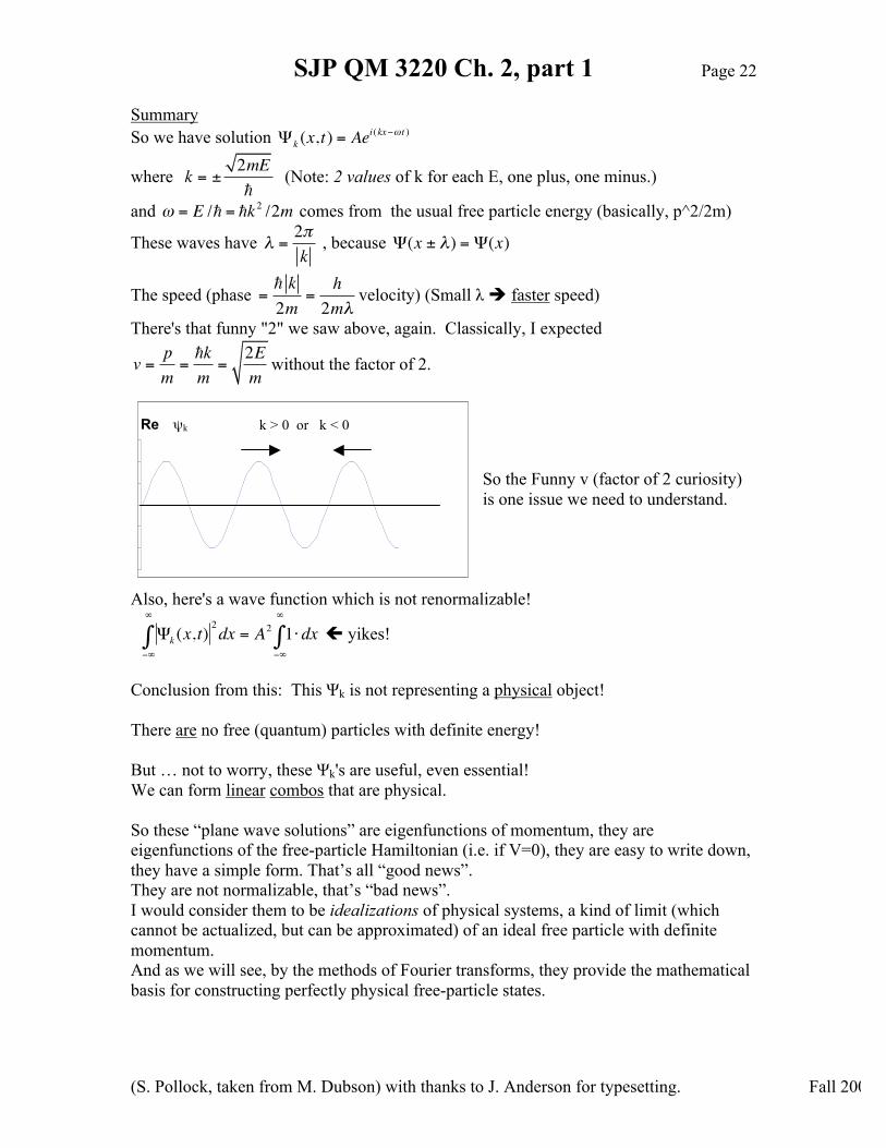
Summary So we have solution Ψk (x,t) = Ae

i(kx−ω t )

where

k = ±2mE

(Note: 2 values of k for each E, one plus, one minus.)

and

€

ω = E / = k 2 /2m comes from the usual free particle energy (basically, p^2/2m)

These waves have λ =2πk

, because Ψ(x ± λ) = Ψ(x)

The speed (phase

= k2m

=h2mλ

velocity) (Small λ faster speed)

There's that funny "2" we saw above, again. Classically, I expected

v =pm=km=

2Em

without the factor of 2.

So the Funny v (factor of 2 curiosity) is one issue we need to understand.

Also, here's a wave function which is not renormalizable!

€

Ψk (x,t)2dx = A2 1⋅ dx

−∞

∞

∫−∞

∞

∫ yikes!

Conclusion from this: This Ψk is not representing a physical object! There are no free (quantum) particles with definite energy! But … not to worry, these Ψk's are useful, even essential! We can form linear combos that are physical. So these “plane wave solutions” are eigenfunctions of momentum, they are eigenfunctions of the free-particle Hamiltonian (i.e. if V=0), they are easy to write down, they have a simple form. That’s all “good news”. They are not normalizable, that’s “bad news”. I would consider them to be idealizations of physical systems, a kind of limit (which cannot be actualized, but can be approximated) of an ideal free particle with definite momentum. And as we will see, by the methods of Fourier transforms, they provide the mathematical basis for constructing perfectly physical free-particle states.

k > 0 or k < 0 Re _ (k) k > 0 or k < 0 ψk



Since k is a continuous variable, combining Ψk's requires not a sum over k, but an integral over k!

Consider

€

Ψgeneralfree (x, t) =

12π

φ(k)Ψk (x,t)dk−∞

∞

∫ =12π

φ(k)ei(kx−Ek t )dk−∞

∞

∫

This looks a little scary, but it’s just the continuous analogue of our old familiar "Fourier" formula:

€

Ψgeneralsquare well (x,t) = cn

n∑ Ψn

square well (x,t) , where we basically replace

€

cn →φ(k)dk

This Ψ has many k's (momenta, energies) superposed.

If I give you

€

Ψgeneral (x,0) =12π

φ(k)eikxdk−∞

∞

∫

then you can figure out φ(k) (like Fourier's trick!) and given φ(k), you then know, from equation at top of page, Ψ at all future times. So we need to review "Fourier's trick" for continuous k! Note Ψk(x,0) = eikx simple enough …

Suppose I give you f(x), and ask "what φ(k) is needed" so that

€

f (x) =12π

φ(k)eikxdx−∞

∞

∫

This is our problem: Given Ψgen(x, t=0), find φ(k). Because once you've got it, you know Ψ at all times.

stuck this in for later convenience

This plays the role of cn before, it's a function of k

Sum over all k's, + or - .

This is the “plane wave”, the eigenstate of energy for a free particle



The answer is Plancherel's Theorem, also known as the "Fourier Transform".

€

φ(k) =12π

f (x)e−ikxdx−∞

∞

∫ (Note the minus sign in the exponential here!)

Recall that if

€

f (x) = cn2asin nπx

an∑ ,then Fourier's trick gave

€

cn = f (x)∫2asin nπx

adx

It's rather similar; the coefficients are integrals of the desired function with our "orthogonal basis" functions.

φ(k) is the "Fourier transform" of f(x) here. If f(x) (here Ψ(x, t=0) is normalizable to start with, Ψ(x,t) will be too, as will φ(k). You can "build" almost ANY FUNCTION f(x) you want this way!!

Digression – Some examples of Fourier transforms. Griffiths (p. 62) has "width" is

€

≈ 2a.

then

€

φ(k) =12π


∞

∫ is easy,

you get

€

φ(k) =1πasinkak

(Do it, try it yourself!)

If a → 0, Need many momenta to build a narrow wave packet If a → ∞, One (sharp) momentum broad wave packet, where is it?

-a -a

f(x)

x

π/a is "width", roughly

f(x) localized

φ(k) ~ constant spread out

f(x) spread out



Digression continued: Let's do another:

€

f (x) = Ae−x2 / 4α

Here

€

12π

f (x)e− ikxdx−∞

∞

∫ can be done analytically (guess what's on the next homework?)

€

φ(k) =A2π

e−

x 2

4α+ ikx )

dx =

−∞

∞

∫A2π

e−k2αe−k

2α e−

x2 α

− ik α

2

dx−∞

∞

∫

(That little trick on the right is called "completing the square", you need to DO that algebra yourself to see exactly how it works, it's a common and useful trick)

Basically, letting

€

x'= x2 α

− ik α ; dx '= dx2 α

; e-x ' 2

dx '= π-∞

∞

∫

you then get

€

φ(k) =2 α2Ae−k

2α

Once again, narrow in f wide in φ, and vice versa. ▪ If f is centered around x0,

€

f (x) = Ae−(x−x0 )2 / 4α

work it out… This will add (well, really multiply!) a phase

€

eikx0 to φ(k). So the phase of φ(k) does carry some important information (but not about momentum itself!) (Puzzle for you: what does a phase

€

eik0x multiplying f(x) do? …)

width ~ 2α

width ~ 1/√α



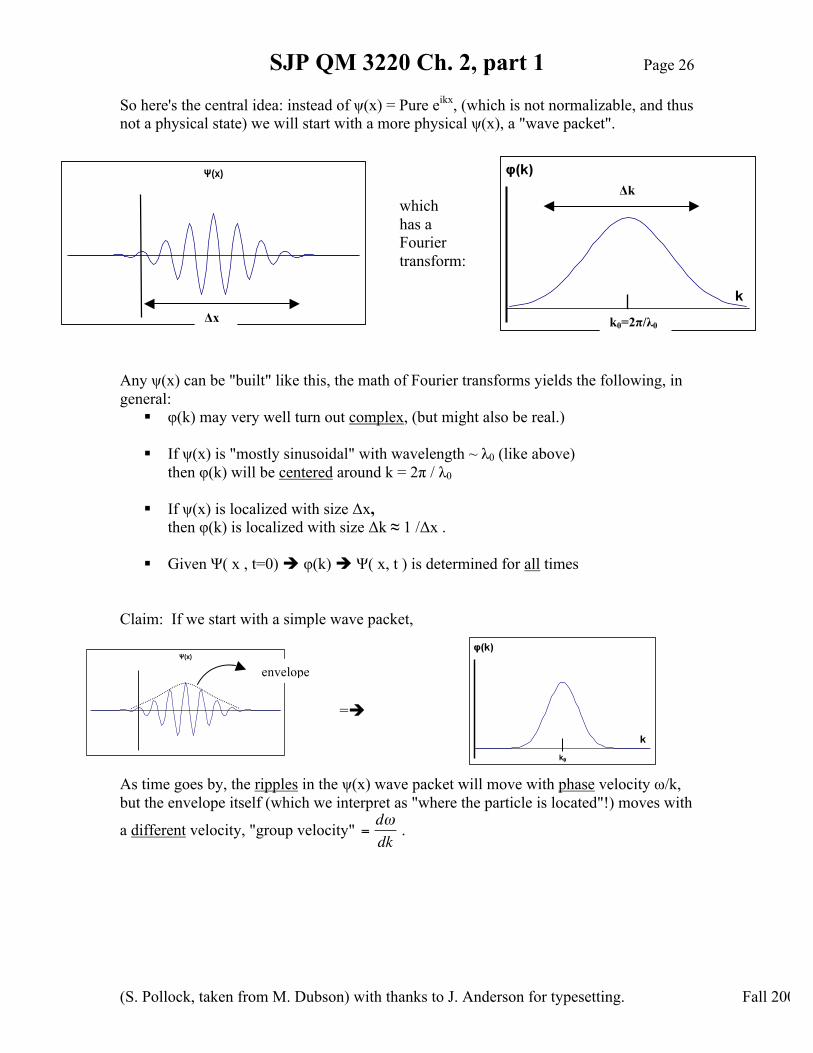
So here's the central idea: instead of ψ(x) = Pure eikx, (which is not normalizable, and thus not a physical state) we will start with a more physical ψ(x), a "wave packet".

Any ψ(x) can be "built" like this, the math of Fourier transforms yields the following, in general:

φ(k) may very well turn out complex, (but might also be real.)

If ψ(x) is "mostly sinusoidal" with wavelength ~ λ0 (like above) then φ(k) will be centered around k = 2π / λ0

If ψ(x) is localized with size Δx, then φ(k) is localized with size Δk ≈ 1 /Δx .

Given Ψ( x , t=0) φ(k) Ψ( x, t ) is determined for all times Claim: If we start with a simple wave packet,

=

As time goes by, the ripples in the ψ(x) wave packet will move with phase velocity ω/k, but the envelope itself (which we interpret as "where the particle is located"!) moves with

a different velocity, "group velocity"

€

=dωdk

.

λ0

which has a Fourier transform:

Δk

k0=2π/λ0

envelope

Δx



DIGRESSION on “phase and group velocity”, and the resolution of the “speed” puzzle. Let’s look more at this last statement, about phase and group velocity.

In our case (a free particle),

€

ω =E

=

2mk 2 , so

dωdk

=km

, no funny factor of 2 present!

This resolves both our "free particle issues":

1) The packet moves with

€

υclassical =km

2) The Ψ( x, t ) is perfectly normalizable. ▪ And something else happens: different k's move with different speeds, so the ripples tend to spread out the packet as time goes by, So → → So Δx grows with time! Let me go back, and make a casual proof of the "claim" above about the time development of a wave packet:

€

Ψgeneral (x, t) =12π

φ(k)ei(kx−ωt )dk−∞

∞

∫

Recall ω is itself dependent on k,

€

ω =k 2

2min this case of a free

particle, it's just a consequence of E = p^2/2m. Let's consider a wave packet where φ(k) is peaked near k0. So we have a "reasonably well-defined momentum, (this is what you think of when you have a real particle like an electron in a beam …) ( If you had many k's, each k travels at different speeds packet spreads, not really a "particle" …) So this is a special case, but a common/practical one … So if k's are localized, consider Taylor expanding ω(k) ω( k ) = ω( k0 ) + ω'(k0 ) ( k - k0 ) + . . . This should be a fine approximation for the ω( k ) in that integral we need to do at the top of the page! Let's define k' ≡ k - k0 as a better integration variable, so dk' = dk, but ω ≈ ω( k0 ) + ω'( k0 ) k' + . . .

higher k's move up front



€

Ψgen (x,t) =12π

φ(k '+k0)eik'xe−iω (k0 )te−w' (k0 )k' t

−∞

∞

∫

= eik0xe− iω (k0 )t 12π

φ(k'+k0)eik' xe−iω ' (k0 )⋅k'⋅t

−∞

∞

∫

= ei(k0x−ω 0t )

12π

φ(k0 + k')eik' (x−ω ' 0 t )

−∞

∞

∫ dk'

These are ripples, This is a function of (x - ω'0 t .) a function of This is the time-evolving envelope, (x – ω0/k0 · t) which travels at speed ω'0

They travel with vphase= ω0/k0 That's the group velocity,

So the quantum free wave packet moves with

€

υ =ω '0 ≅k0

m

Just as you'd expect classically. The ripples travel at vphase, but | ψ |2 don't care about the ripples, really. Wave packets do "spread out" in time, we could compute this (turns out it spreads faster if starts out narrower!) END OF DIGRESSION. (Which showed how group and phase velocities are different, how wave packets DO behave classically, and how they represent physical particles) At this point we're armed to solve a variety of general quantum mechanics problems: Given V(x), (and ψ(t=0)), find Ψ( x, t ). That’s huge! → Bound states will generate discrete En's and un's (this is the story we started the term with – like the harmonic oscillator, or the infinite square well) The time dependence is especially interesting when you start with “mixed states” → Free particles will become "scattering states". This is what we’ve just gotten started. We'll talk more about this soon, at which point we’ll go back and tackle a few more simple problems, to get familiar with the Ψ's for “scattering states”.



But first, let’s talk about the INTERPRETATION of our Fourier transform: what does φ(k) mean? It plays an important role in Quantum Mechanics, and will lead us to even more powerful ways of thinking about wave functions. We’ve already danced around it - φ(k) is the “momentum distribution”, it tells you about the particle in “momentum space”, it’s a probability distribution for momentum! Let’s see how this works: To begin, consider again the general (math!) formulas for Fourier transform and inverse:

€

f (x) =12π

φ(k)e+ikxdk−∞

∞

∫

€

φ(k) =12π


∞

∫

Now, consider the Fourier transform of a δ function, i.e. let f(x)=δ(x), so (from above)

€

φ(k) =12π

δ(x)e−ikxdx−∞

∞

∫ =12π

(The last step is pure math - integrating δ(x) gives

you the rest of the integrand evaluated at the point where the argument of δ(x) vanishes) But now the inverse of this (just read it off from the Fourier formulas above!) says:

€

f (x) = δ(x) =12π

φ(k)e+ ikxdk−∞

∞

∫ =12π

e+ ikxdk−∞

∞

∫ Let me “name” this relation (1)

It’s strange - the integral on the right looks awful. It oscillates forever, is it really defined? Well, it’s a little dicey (you do need to be careful how you apply it), but basically, if x is NOT 0 the “oscillating integrand” gives zero (think of real and imaginary parts separately, the area under a “sinusoidal function” is zero), but if x is zero, you integrate “1” over all space and get infinity. That’s the delta function! OK, armed with this identity, consider any normalized wave function Ψ(x), for which

€

Ψ* (x)−∞

∞

∫ Ψ(x)dx =1 . Let’s write Ψ(x)=

€

12π

φ(k)e+ ikxdk−∞

∞

∫ (which you can

ALWAYS do), so here φ(k) is just the usual Fourier transform of Ψ(x). We’ll put this formula for Ψ(x), into the normalization integral, (twice, once for Ψ(x) and once for Ψ∗(x).) Just be careful to change dummy indices for the second one!

€

12π

φ(k)e+ikxdk−∞

∞

∫

*

−∞

∞

∫ 12π

φ(k')e+ik'xdk '−∞

∞

∫

dx =1

That’s a triple integral (ack!) but check it out, the only x-dependence is in TWO places, the two exponentials. So let’s pull that x dependence aside and do the x-integration first:

€

e−ikxe+ik'xdx 12π

φ(k)dk−∞

∞

∫

*

−∞

∞

∫ 12π

φ(k ')dk '−∞

∞

∫

=1

(Note the “–“ sign in the ikx term came from the complex conjugation. Follow the algebra here, don’t take my word for anything!)



But I can DO that integral over x: just use our cute integral (1) to simplify. Let me first take integral (1) and rewrite it, flipping x’s and k’s:

€

δ(k) =12π

e+ikxdx−∞

∞

∫ (1’) (Convince yourself, treat x and k as pure symbols!)

But this is precisely what I have in my triple integral, except instead of k I have (k’-k). Substitute this in (getting rid of the dx integral, which “eats up” the Sqrt[2π] terms too!)

€

δ(k'−k)φ * (k)φ(k ')dk dk '∫∫ =1 (It’s easy to “glaze over” this kind of math. Pull out a piece of paper and DO it, the steps are not hard, and you’ll use these tricks many times. Check that you see what happened to the 2π‘s and the integral over x) There’s still a double integral over k and k’, but with the δ(k’-k) it’s easy enough to do, I love integrating over δ’s! Let’s integrate over k’, and collapse it with the δ, giving

€

φ * (k)φ(k)dk−∞

∞

∫ =1 Ah – this is important. We started with a normalized wave function Ψ(x), and what I just showed is that the Fourier transform, φ(k) , is ALSO normalized. But there’s more! Consider now

€

p = Ψ* (x)−∞

∞

∫

i∂∂x

Ψ(x)dx . Play the exact same game as before, but with that

derivative (d/dx) inside. All it will do will pull out an ik’ (convince yourself), everything else looks like what I just did, and we get

€

p = (k)φ * (k)φ(k)dk−∞

∞

∫ . Now, deBroglie identifies

€

k with p. So just stare at this until you realize what it’s saying. I would expect (from week 1!) that

€

p = p Prob density(p)dp−∞

∞

∫ . So here it is, apparently (other than annoying factors of

€

, since p and k are essentially the same thing, p=

€

k) we know what the “Probability density for momentum” is, it’s just

€

φ * (k)φ(k) = φ(k) 2 .

To get the

€

’s right, I would define

€

Φ(p) =1φ(k) , again with p=

€

k . I’ll let you

convince yourself that Φ(p) is properly normalized too,

€

1= Φ* (p)Φ(p)dp−∞

∞

∫ , and

€

p = pΦ* (p)−∞

∞

∫ Φ(p)dp We’ve just done a lot of math, so let’s pull this all together and summarize



Bottom line: We’d gotten used to thinking about Ψ(x) as “the wave function”. When you square it, you learn the probability density to find a particle at position x. Expectation values tell us about OTHER things (any other operator/measurable you want.) Ψ(x) contains ALL information about a quantum particle. Now we have the

Fourier transform, φ(k), or equivalently

€

Φ(p) =1φ(k) . This function depends on “p”.

It contains the SAME information as Ψ(x)! It just lives in “momentum space” instead of “position space”. It’s a function of p.

• Φ(p) is normalized, just like Ψ(x) was. • |Φ(p)|^2 tells the “probability density of finding the particle with momentum p” • Φ(p) is the wave function too. There’s nothing special about x! Φ(p) is called the

“momentum space wave function”. • We can compute expectation values in momentum space to learn about anything,

just like we could before. Let’s now consider this in more detail: We already know

€

p = pΦ* (p)−∞

∞

∫ Φ(p)dp In fact, it shouldn’t be hard to convince yourself that for any function of momentum f(p),

€

f (p) = f (p)Φ* (p)−∞

∞

∫ Φ(p)dp. How about <x>? Here again, start with the usual old formula in terms of Ψ(x) and play the same math game as on the previous pages: expand Ψ(x) as a Fourier transform, you get a triple integral, do the “δ-function” trick, and (try this, it’s not so hard!) you find

€

x = Φ* (p) i ∂∂p−∞

∞

∫ Φ(p)dp.

Look at that for a second. There’s a lovely symmetry here:

In position space, we’ve used

€

ˆ x = x and

€

ˆ p = −i ∂∂x

. Now we’re seeing that

in momentum space,

€

ˆ x = i ∂∂p

, and

€

ˆ p = p .

It’s almost perfect “symmetry” (except for a minus sign, but don’t forget, the inverse Fourier transform has an extra minus sign in front of the “ikx”, which is the source) We will discover there are other “spaces” we might live in. Energy-space comes to mind, but pretty much any-operator-you-like-space can be useful too! The momentum-space example will be the first of many! But for now we move back to our central problem, solving the Schrodinger equation. We’ve done two “bound states”, and the free particle. Next we will consider particles with positive energy (so, they’re still “free”) but where V is not just simply 0 everywhere. This is still a lot LIKE the free particle, it’s a “free particle interacting with things”. This is getting to be real physics, like the beam of protons at LHC interacting with nuclei! We’ll still stick to one dimension (your beam can only go forward and backward, you can only transmit or reflect – no “scattering off at 27 degrees” just yet!) And, at the same time, we will tackle other “bound state” problems too - to keep the math simple, we’ll consider examples with “piecewise constant” V(x), like in the picture on the next page:



Back to our problem, in general, of solving the TISE, Schrodinger‘s equation:

€

ˆ H un (x) = Enun (x), or writing it out : − 2

2md2

dx 2 u(x) + V (x)u(x) = Eu(x)

€

u' '(x) = −2m2 (E −V (x))u(x). So u and u' need to be continuous, at least if V is finite.

If E > V(x), that means u'' = - (k2) u Classically, KE > 0

€

k 2 ≡2m(E −V )

2 , or E −V =

2k 2

2m

De Broglie=

p2

2m

asusual!

u'' = - k2 u => curvature is towards axis. This is a wiggly function! If k2 is constant, u = A sin kx + B cos kx or = A' eikx + B' e-ikx Big K.E. Big k2 more wiggly (smaller λ) Classically Big K.E. faster speed less likely to be found there. This is very different, it corresponds in QM not to λ, but amplitude. ← (well, usually, but there are exceptions) So as a specfic example:

V(x)

x L

slow fast

V(x)

I expect ===

E smaller k longer λ

Big k small λ

L x

low prob small | ψ|

higher prob big |ψ|

V(x)

x

V(x)

E<v

(KE) E>V E



What if E < V? Classically this never happens (negative K.E.?!)

In Q.M.,

€

u' '(x) = −2m2 (E −V (x)) ⋅ u(x)

If E < V, define

€

κ = +2m(V − E)

, so u' '= +κ 2u

This is not wiggly, curvature is away from axis. If κ2 = constant (constant V in a region) u(x) = C e- κx + D e + κx . The other signs, e.g. e + κx for x > 0 blow up at ∞, no good! So in the "classically forbidden" regions, can have u(x) ≠ 0. But, u → 0 exponentially fast. So e.g. d= "Penetration depth"

€

= 1κ = 2m(V − E) If V>>E, rapid decay!

E

classical turning point

E < V here

V(x)

x L

E

V(x)

x L (L+d)

e-κx sinusoidal here

e+ κx is good if x < 0

e- κx is good if x > 0



With just these ideas, you can guess/sketch u(x) in many cases: u, u' continuous always (if V, E finite) E>V sinusoidal. Bigger E – V smaller λ and usually smaller | ψ | E < V decaying exponential. Bigger V – E faster decay Example: Finite square well continuous spectrum (free) Discrete spectrum (bound) u1(x) x u2(x) Let's work this out more rigorously to check, ok? Let V(x) = 0 - a < x < a Note: I shifted the +V0 outside zero w.r.t Griffiths Assume 0 < E < V0 , i.e. bound state

E2

V(x)

E1

Ground state, even about center Turns out, you can prove, if V(x) is even, V(x)=V(-x), then u(x) must be even or odd, so |u(x)|2 is symmetric!

Very rapid decay (exponential)

1st excited state, 1 node, odd

less rapid decay, more "leaking"

sinusoidal



Let's start with even solutions for u(x): Region Region Region Boundary conditions: Continuity of u at x=+a:

€

uIII(x) |x=+a= uII(x) |x=a Continuity of u' at x=+a:

€

u'III (x) |x=+a= u'II (x) |x=a

(Conditions at x = - a add no new info, since we've already used fact that u is even!) coefficients We have 3 unknowns: E and (A and C) The energy eigenvalue. We have 2 boundary conditions and normalization, so we can solve for 3 unknowns! Continuity of u says

€

Ce−Ka = Acoska Continuity of u' says

€

−KCe-Ka = −Ak sinka Dividing these

€

−K = −k tanka

€

tan2mE

a

−

Kk

=V0 − EE

(A nasty, transcendental equation with one variable, E)

E

V(x)

-a a x

I

II

III

Region

We've solved for u(x) in each region already

I

No good, blows up

II

No good, looking for even solution right now

III

Same C, 'cause looking for even solution!



Can solve that transcendental equation numerically, or graphically,

€

Let z ≡ ka =2mE

2 a

Let z0 =2mV0

2 a

so

€

V0E

=z0z

2

So we want

€

tan z = (z0 /z)2 −1

I see there are solutions for z (which in turn means E, remember, z and E are closely related, by definition, if you know one you know the other) They are discrete. There is a finite number of them. No matter what z0 is, there's always at least solution. (Look at the graph!) If V0 → ∞, solutions are near π/2, 3 π/2, …

Giving

€

E =

2

2ma2 Z2 =

2π 2

2m(2a)2 (12, or 32, …)

which is exactly the even solutions for our ∞ well with width 2a. Knowing z E k and K , our B.C.'s give A in terms of C, and normalization fixes C. I leave the odd solutions to you. The story is similar and you will get, as your

transcendental equation,

€

cot(ka) = −Kk

This time, it's not always the case there's even a single solution. (The well needs to be deep enough to get a 1st excited state, but even a shallow well has one bound state.)



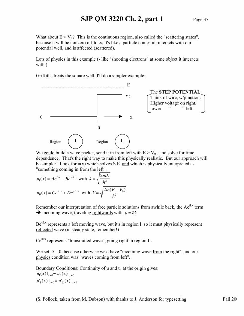
What about E > V0? This is the continuous region, also called the "scattering states", because u will be nonzero off to ∞, it's like a particle comes in, interacts with our potential well, and is affected (scattered). Lots of physics in this example (- like "shooting electrons" at some object it interacts with.) Griffiths treats the square well, I'll do a simpler example: We could build a wave packet, send it in from left with E > V0 , and solve for time dependence. That's the right way to make this physically realistic. But our approach will be simpler. Look for u(x) which solves S.E. and which is physically interpreted as "something coming in from the left".

€

uI(x) = Aeikx + Be− ikx with k =2mE2

uII(x) = Ceik'x + De−ik'x with k'= 2m(E −V0)2

Remember our interpretation of free particle solutions from awhile back, the Aeikx term incoming wave, traveling rightwards with

€

p = k Be-ikx represents a left moving wave, but it's in region I, so it must physically represent reflected wave (in steady state, remember!) Ceik'x represents "transmitted wave", going right in region II. We set D = 0, because otherwise we'd have "incoming wave from the right", and our physics condition was "waves coming from left". Boundary Conditions: Continuity of u and u' at the origin gives:

€

uI(x) |x=0= uII(x) |x=0

u'I (x) |x=0= u'II (x) |x=0

E

V0

Region

x

I

II

0

0

Region

The STEP POTENTIAL. Think of wire, w/junction: Higher voltage on right, lower ˝ ˝ left.



What about normalization? These are not normalizable u's, (like the free particle, you must make a "wave packet" if you want it to be normalized.) But wait, what are we after? Well, given A (= amplitude entering) I want to know, T, "Transmission Coefficient" and R, "Reflection Coefficient", how much of an incident wave moves on, and how much "bounces"? Intuitively, B/A will tell us about R and C/A will tell us about T. Really, R, and T are "the physics" we're after. We need to be careful, I said "tell us about", but it's not "equal", we'll have to come back to R and T in a minute…Let's first compute these ratios, though. Boundary condition on u(x) at x=0 gives A + B = C (Because

€

e± ik⋅0 = 1 ) B.C. on u' gives k ( A - B ) = k' C Now divide by k, add the two equations,

So I get (check!) 2 A = C ( 1 + k'/k) or

€

CA

=2

1+ k' /k

Put this back into 1st equation:

€

A + B = C =2

1+ k' /kA , which then means (again, check

that you follow this algebra, it's not hard, and worth doing)

€

BA

=2

1+ k' /k−1=

1− k ' /k1+ k ' /k

with

€

k'k

=E −V0E

OK, so we know what B/A and C/A are. Now we can talk about interpreting these coefficients of (non-normalizable) "plane waves".



Probability Current J(x,t). |ψ|2 evolves with time, smoothly. So probability "flows" in (and out) of this region!

I claim

€

∂∂tψ (x,t) 2 = −

∂∂x

J(x, t)( ) , and this J function is called "Probability current"*

where

€

J(x, t) =i2m

ψ∂ψ *

∂x−ψ * ∂ψ

∂x

You need to do the algebra in prev. equation!

Let's rewrite the first "claimed" equation as

€

∂P∂t

+∂J∂x

= 0where P = Prob. density = | ψ |2

or, integrating a → b

€

∂∂t

P ⋅ dxa

b

∫

= −∂J∂xdx = − (J(b) − J(a)) = J(a) − J(b)

a

b

∫

rate of "buildup" = "current in at a " – "current out at b" in (a,b) region * Just like electric charge, the name "current" is good!

Note that

€

J(x, t) =i2m

(−2i) ⋅ Im ψ * ∂ψ∂x

=

mIm ψ * ∂ψ

∂x

For a plane wave ,

€

Ψ = Aei(kx−ωt )

€

∂Ψ∂x

= ikΨ, so J =

mIm ikΨ*Ψ( ) , which means (again, for a plane wave),

€

J =

mA 2k

This is key:

€

km

looks like pm

= v

So "flow of probability" in a plane wave is like v · |A|2 Think of electric current, where j = ρ v Very similar! |A|2 plays the role of "charge density" here.

large amp. lots of flow fast movement

lots of flow

charge density

speed of charge



So back to our scattering problem, with particles coming in from the left and hitting a "step up" potential, but with E>V: If J = "probability current", then

R= reflection coefficient =

€

JrefJinc

€

which is just B 2 /A 2 , do you see that from the formula

for J we got on the previous page?

T= Transmission coefficient =

€

JtransJinc

, which is NOT

€

C 2 /A 2 , it is

€

JtransJinc

=C 2

A 2k'k

(Think a little about the presence of the k'/k term there - I might not have expected it at first, thinking maybe T = C2/A2, but when you look at our probability current formula, you realize it makes sense, the waves have a different speed over there on the right side, and probability current depends not JUST on amplitude, but ALSO on speed!) We solved for B/A and C/A, so here

€

R =1− k '

k1+ k '

k

2

T =4

1 + k 'k( )2 ⋅

k 'k

convince yourself then, that R + T =1 (!) Convince yourself

Note: If V0 → 0 ,

€

k'k

=E −V0E

→1 (Convince yourself!) and then check, from the

formulas above, that R → 0 and T → 1 . This makes sense to me - there's no barrier in this limit!

On the other hand, if E → V0, I claim

€

k'k→ 0 (again, do you see why?), and in THIS

limit, the formulas above tell us that R→1 and T→0. Again, this makes sense - in this limit, it is "forbidden" to go past the barrier. (Classically, if E > V0, R = 0. QM gives something new here.)

E0

V0

Jref

C Jtransmitted

Jinc

B

A



Other examples: Pain, but can compute R, T. E < V0: T is not 0, even though classically it would be. This is tunneling. E > V0: Classically, T=1, but QM some reflection.

E V0 V

SJP QM 3220 Ch. 2, part 1 Page 1 Once again, the...

Documents

Transcript of SJP QM 3220 Ch. 2, part 1 Page 1 Once again, the...