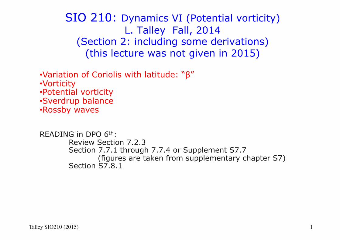
SIO 210: Dynamics VI (Potential vorticity) L. Talley Fall, 2014

(Section 2: including some derivations) (this lecture was not given in 2015)

Talley SIO210 (2015) 1

• Variation of Coriolis with latitude: “β” • Vorticity • Potential vorticity • Sverdrup balance • Rossby waves

READING in DPO 6th: Review Section 7.2.3 Section 7.7.1 through 7.7.4 or Supplement S7.7 (figures are taken from supplementary chapter S7) Section S7.8.1

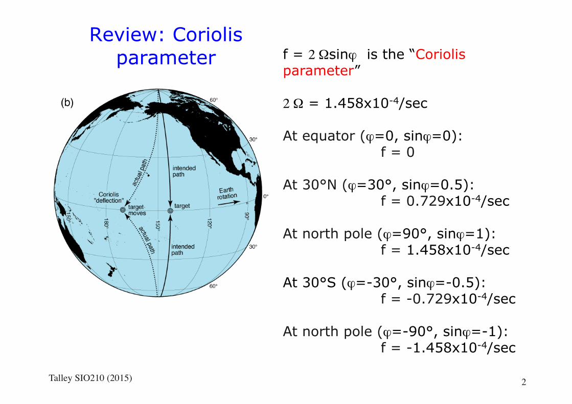
Review: Coriolis parameter f = 2 Ωsinϕ is the “Coriolis

parameter”

2 Ω = 1.458x10-4/sec

At equator (ϕ=0, sinϕ=0): f = 0

At 30°N (ϕ=30°, sinϕ=0.5): f = 0.729x10-4/sec

At north pole (ϕ=90°, sinϕ=1): f = 1.458x10-4/sec

At 30°S (ϕ=-30°, sinϕ=-0.5): f = -0.729x10-4/sec

At north pole (ϕ=-90°, sinϕ=-1): f = -1.458x10-4/sec

Talley SIO210 (2015) 2

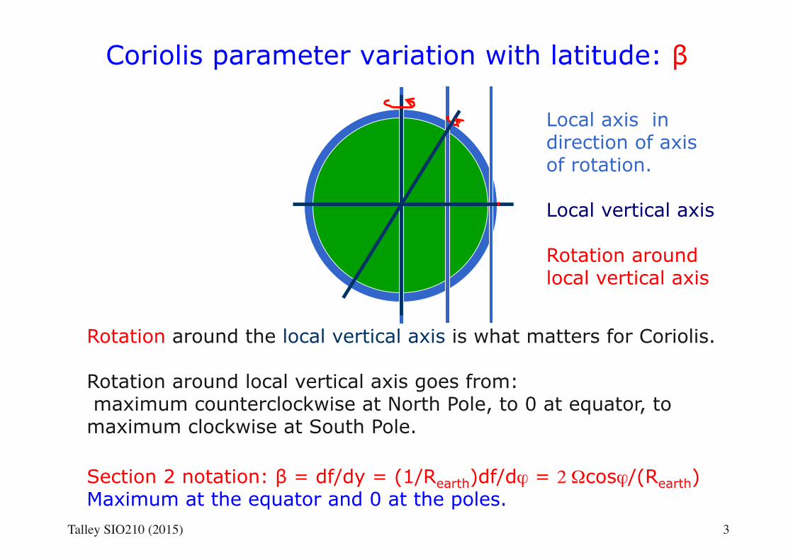
Coriolis parameter variation with latitude: β

Talley SIO210 (2015) 3

Rotation around the local vertical axis is what matters for Coriolis.

Rotation around local vertical axis goes from: maximum counterclockwise at North Pole, to 0 at equator, to maximum clockwise at South Pole.

Section 2 notation: β = df/dy = (1/Rearth)df/dϕ = 2 Ωcosϕ/(Rearth) Maximum at the equator and 0 at the poles.

Local axis in direction of axis of rotation.

Local vertical axis

Rotation around local vertical axis

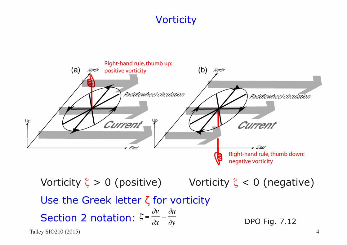
Vorticity

Vorticity ζ > 0 (positive)

Use the Greek letter ζ for vorticity

Section 2 notation:

Vorticity ζ < 0 (negative)

DPO Fig. 7.12 Talley SIO210 (2015) 4

€

ζ =∂v∂x

−∂u∂y

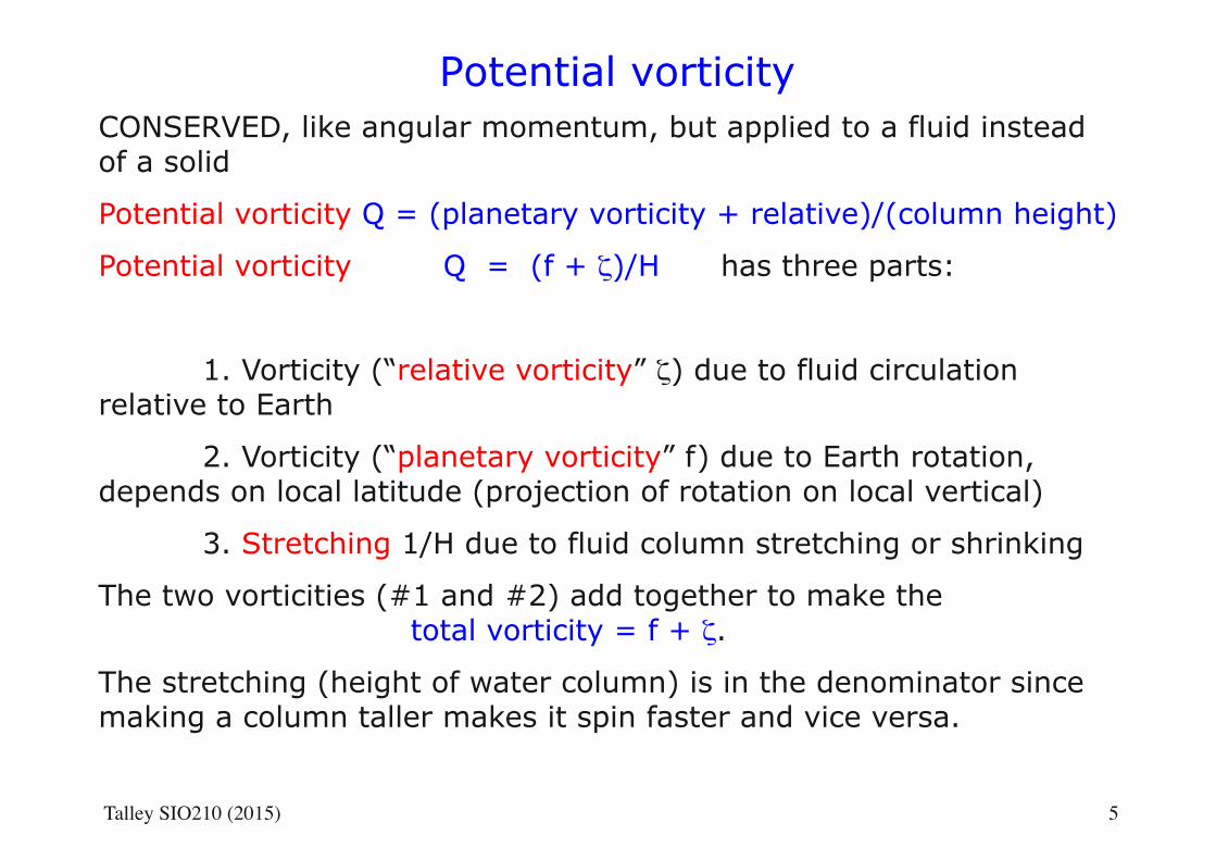
Potential vorticity CONSERVED, like angular momentum, but applied to a fluid instead of a solid

Potential vorticity Q = (planetary vorticity + relative)/(column height)

Potential vorticity Q = (f + ζ)/H has three parts:

1. Vorticity (“relative vorticity” ζ) due to fluid circulation relative to Earth

2. Vorticity (“planetary vorticity” f) due to Earth rotation, depends on local latitude (projection of rotation on local vertical)

3. Stretching 1/H due to fluid column stretching or shrinking

The two vorticities (#1 and #2) add together to make the total vorticity = f + ζ.

The stretching (height of water column) is in the denominator since making a column taller makes it spin faster and vice versa.

Talley SIO210 (2015) 5

Vorticity equation (Section 2 derivations)

Talley SIO210 (2015) 6

€

DuDt

− fv = −1ρo

∂p∂x

+ AH∇H2u + AV

∂ 2u∂z2

DvDt

+ fu = −1ρo

∂p∂y

+ AH∇H2v + AV

∂ 2v∂z2

x, y momentum equations(Boussinesq approximation, using ρo in x,y)

To form vorticity equation: cross-differentiate and subtract to eliminate the pressure terms. (Have approximated the D/Dt as horizontal terms only.)

€

−∂∂y∂∂x

€

DζDt

+ ( f +ζ)(ux + vy ) + βv = AH∇2ζ + AV

∂ 2ζ∂z2

+O(Ro)

ζ = (vx-uy)

Use continuity ux+vy+wz= 0 to substitute and yield

€

DζDt

− ( f +ζ)wz + βv = 0 + AH∇2ζ + AV

∂ 2ζ∂z2

Vorticity equation

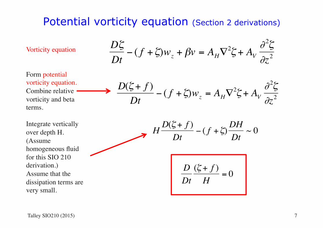
Potential vorticity equation (Section 2 derivations)

Talley SIO210 (2015) 7

€

DζDt

− ( f +ζ)wz + βv = AH∇2ζ + AV

∂ 2ζ∂z2

Vorticity equation

Form potential vorticity equation. Combine relative vorticity and beta terms.

Integrate vertically over depth H. (Assume homogeneous fluid for this SIO 210 derivation.)Assume that the dissipation terms are very small.

€

D(ζ + f )Dt

− ( f +ζ)wz = AH∇2ζ + AV

∂ 2ζ∂z2

€

H D(ζ + f )Dt

− ( f +ζ)DHDt

~ 0

€

DDt(ζ + f )H

= 0

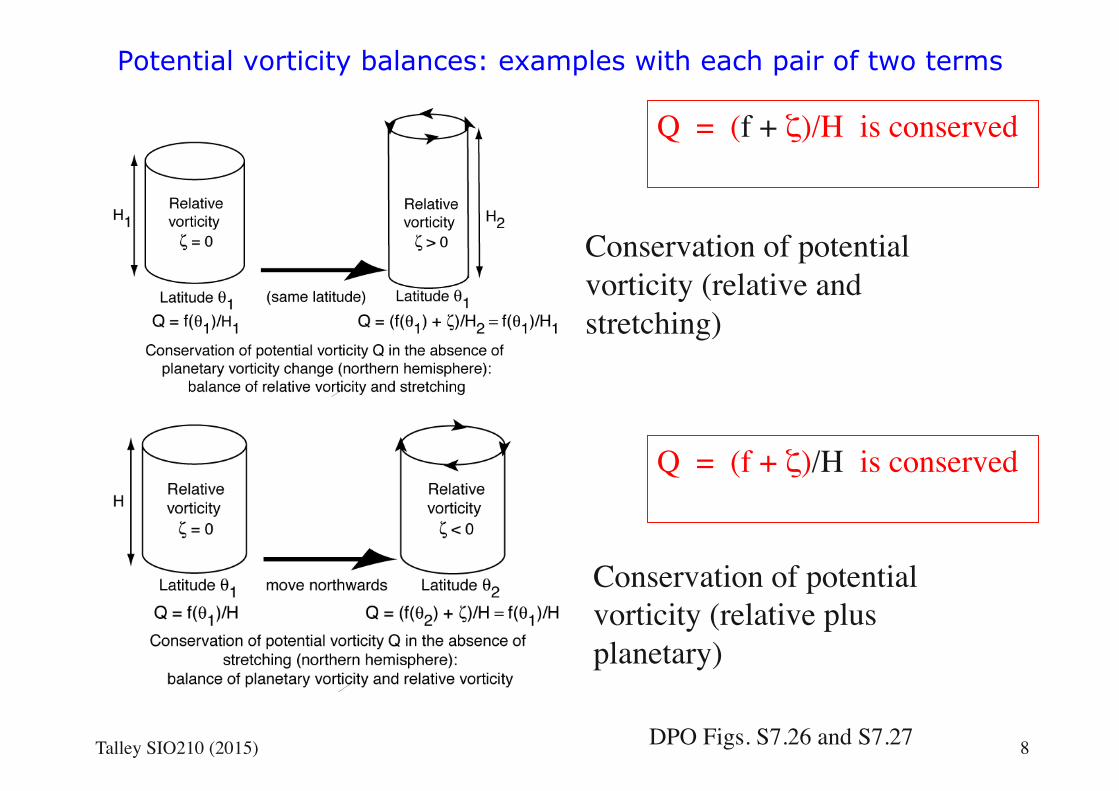
Potential vorticity balances: examples with each pair of two terms

Conservation of potential vorticity (relative plus planetary)

Conservation of potential vorticity (relative and stretching)

DPO Figs. S7.26 and S7.27

Q = (f + ζ)/H is conserved

Talley SIO210 (2015)

Q = (f + ζ)/H is conserved

8

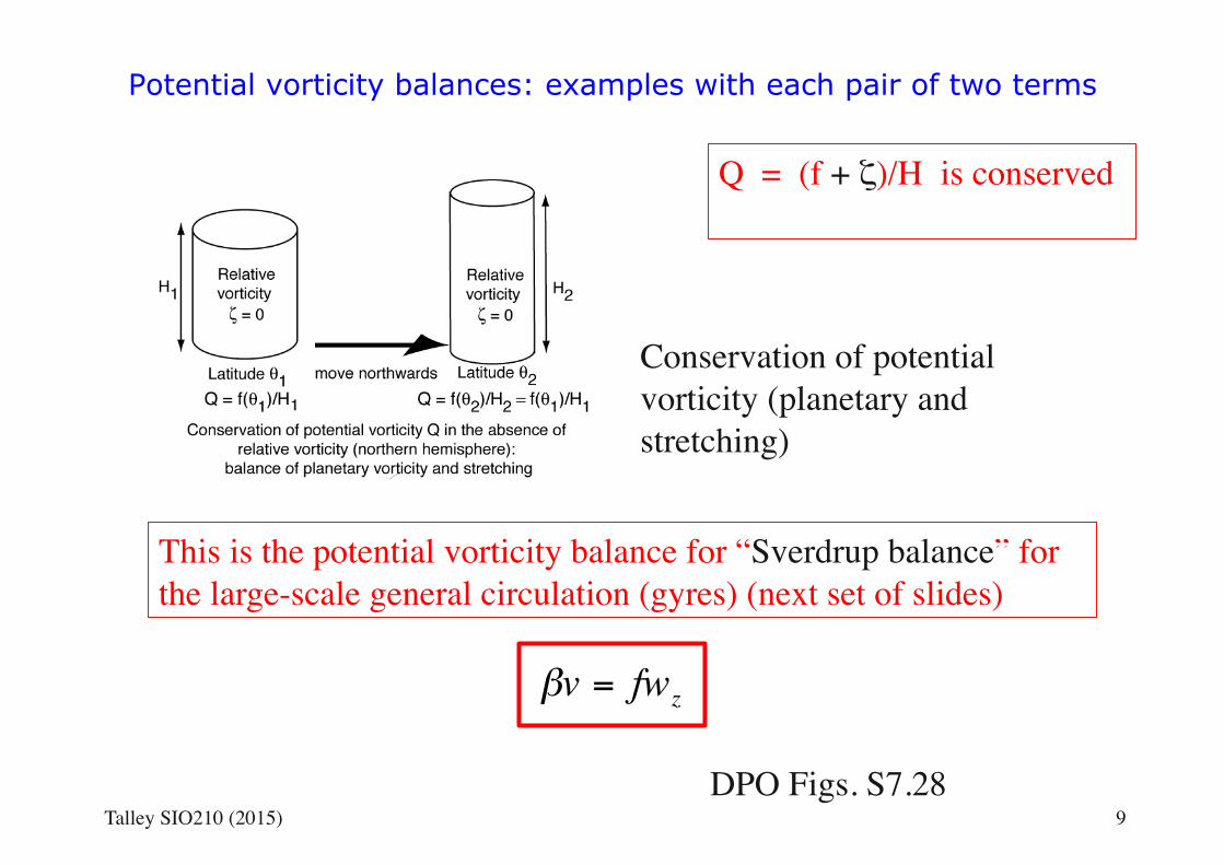
Potential vorticity balances: examples with each pair of two terms

Conservation of potential vorticity (planetary and stretching)

This is the potential vorticity balance for “Sverdrup balance” for the large-scale general circulation (gyres) (next set of slides)

DPO Figs. S7.28Talley SIO210 (2015)

Q = (f + ζ)/H is conserved

9

€

βv = fwz

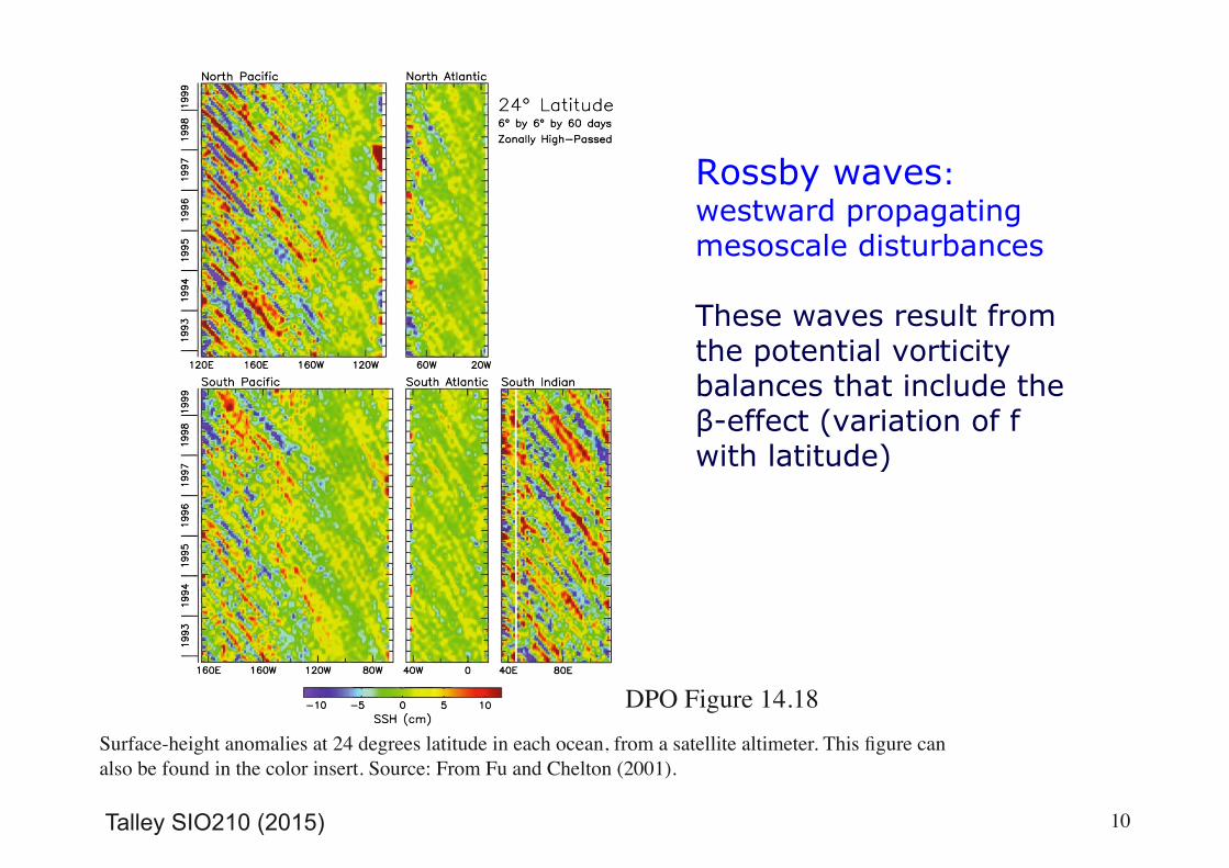
Rossby waves: westward propagating mesoscale disturbances

These waves result from the potential vorticity balances that include the β-effect (variation of f with latitude)

Talley SIO210 (2015)

Surface-height anomalies at 24 degrees latitude in each ocean, from a satellite altimeter. This figure can also be found in the color insert. Source: From Fu and Chelton (2001).

10

DPO Figure 14.18

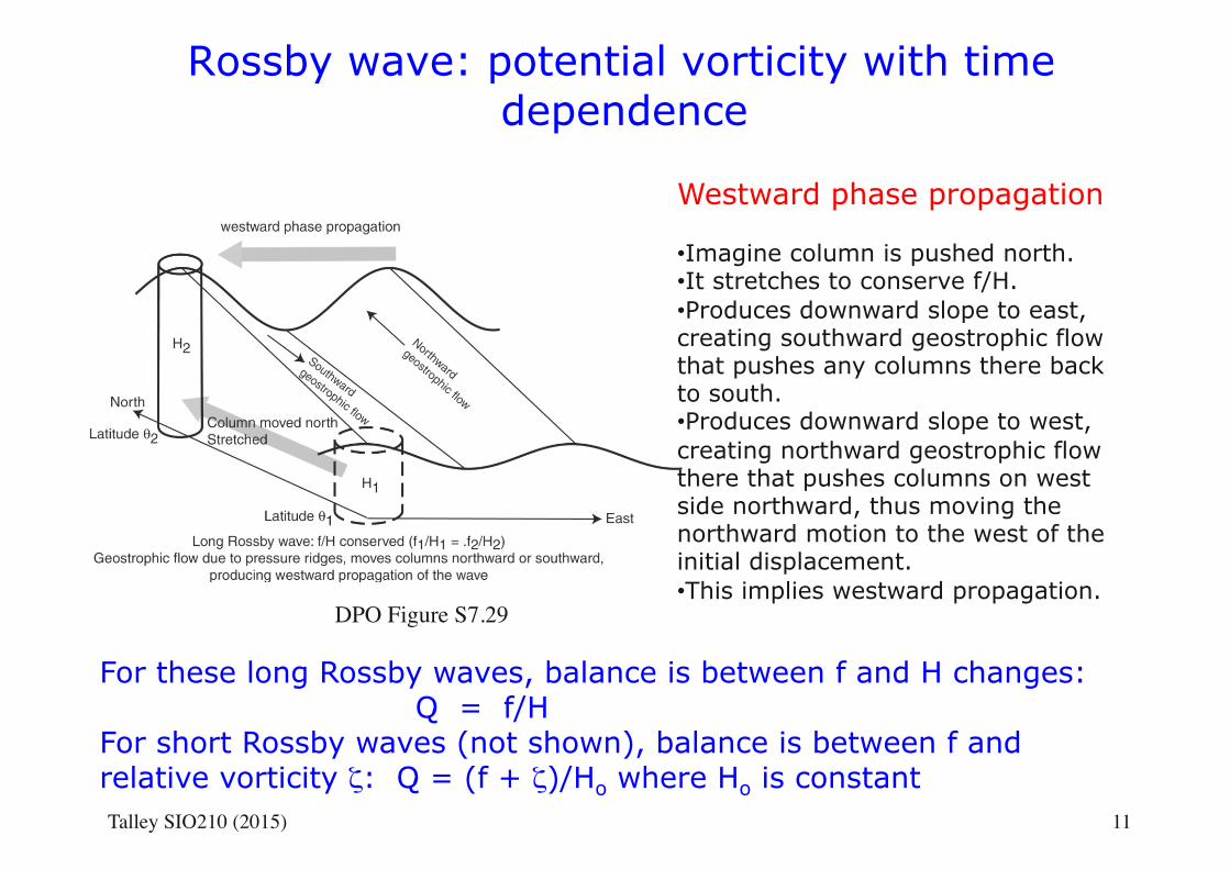
Rossby wave: potential vorticity with time dependence

For these long Rossby waves, balance is between f and H changes: Q = f/H

For short Rossby waves (not shown), balance is between f and relative vorticity ζ: Q = (f + ζ)/Ho where Ho is constant

11Talley SIO210 (2015)

Westward phase propagation

• Imagine column is pushed north. • It stretches to conserve f/H. • Produces downward slope to east, creating southward geostrophic flow that pushes any columns there back to south. • Produces downward slope to west, creating northward geostrophic flow there that pushes columns on west side northward, thus moving the northward motion to the west of the initial displacement. • This implies westward propagation.

DPO Figure S7.29

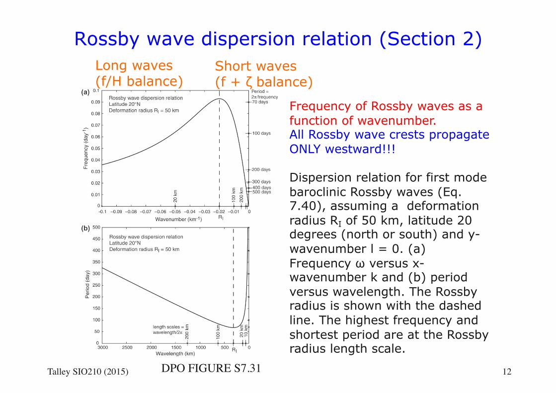
DPO FIGURE S7.31

Frequency of Rossby waves as a function of wavenumber. All Rossby wave crests propagate ONLY westward!!!

Dispersion relation for first mode baroclinic Rossby waves (Eq. 7.40), assuming a deformation radius RI of 50 km, latitude 20 degrees (north or south) and y-wavenumber l = 0. (a) Frequency ω versus x-wavenumber k and (b) period versus wavelength. The Rossby radius is shown with the dashed line. The highest frequency and shortest period are at the Rossby radius length scale.

Rossby wave dispersion relation (Section 2) Long waves (f/H balance)

Short waves (f + ζ balance)

12Talley SIO210 (2015)

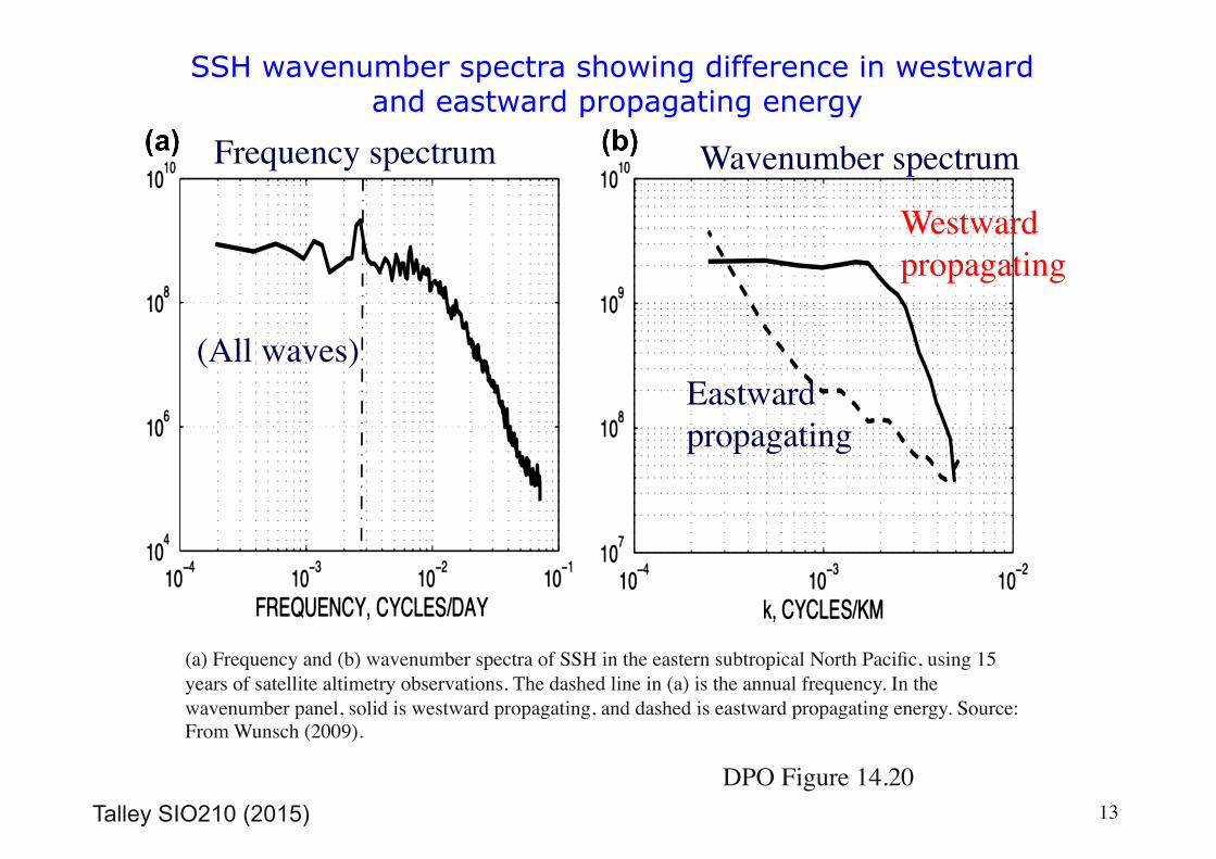
SSH wavenumber spectra showing difference in westward and eastward propagating energy

Talley SIO210 (2015)

(a) Frequency and (b) wavenumber spectra of SSH in the eastern subtropical North Pacific, using 15 years of satellite altimetry observations. The dashed line in (a) is the annual frequency. In the wavenumber panel, solid is westward propagating, and dashed is eastward propagating energy. Source: From Wunsch (2009).

13DPO Figure 14.20

Westward propagating

Eastward propagating

Wavenumber spectrumFrequency spectrum

(All waves)

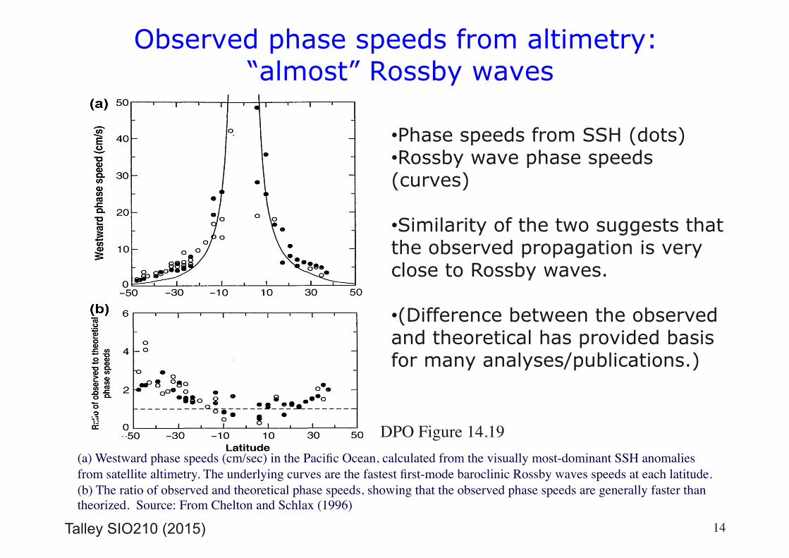
Observed phase speeds from altimetry: “almost” Rossby waves

Talley SIO210 (2015)

TALLEY

14

• Phase speeds from SSH (dots) • Rossby wave phase speeds (curves)

• Similarity of the two suggests that the observed propagation is very close to Rossby waves.

• (Difference between the observed and theoretical has provided basis for many analyses/publications.)

DPO Figure 14.19(a) Westward phase speeds (cm/sec) in the Pacific Ocean, calculated from the visually most-dominant SSH anomalies from satellite altimetry. The underlying curves are the fastest first-mode baroclinic Rossby waves speeds at each latitude. (b) The ratio of observed and theoretical phase speeds, showing that the observed phase speeds are generally faster than theorized. Source: From Chelton and Schlax (1996)

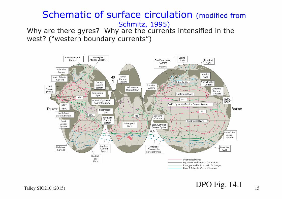
Schematic of surface circulation (modified from Schmitz, 1995)

Why are there gyres? Why are the currents intensified in the west? (“western boundary currents”)

DPO Fig. 14.1Talley SIO210 (2015) 15

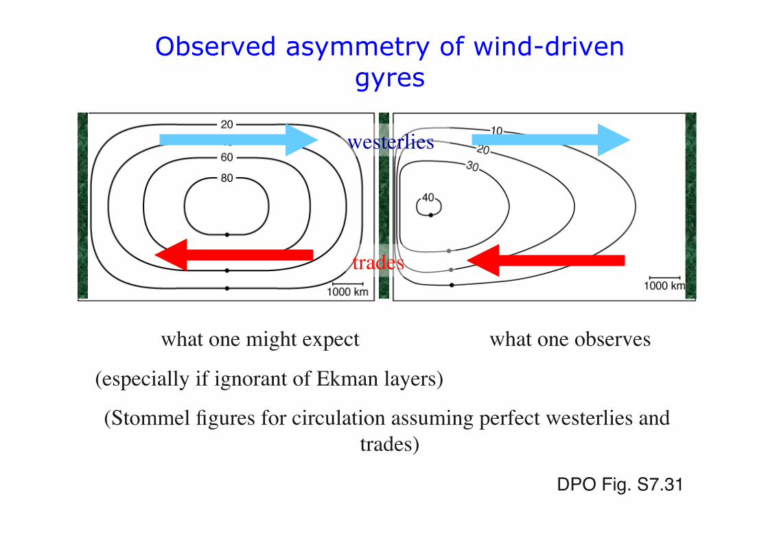
Observed asymmetry of wind-driven gyres

what one might expect what one observes

(especially if ignorant of Ekman layers)

(Stommel figures for circulation assuming perfect westerlies and trades)

DPO Fig. S7.31

westerlies

trades

= LAND

Talley SIO210 (2015) 16

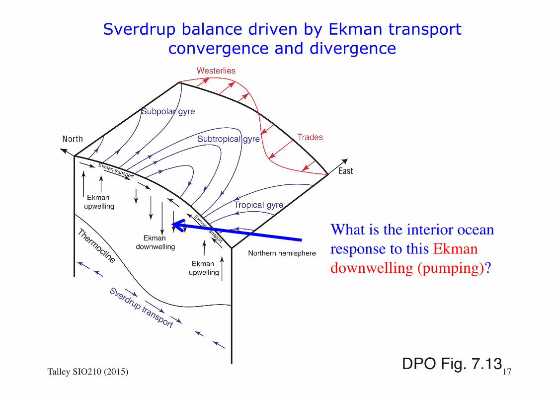
Sverdrup balance driven by Ekman transport convergence and divergence

DPO Fig. 7.13Talley SIO210 (2015)

What is the interior ocean response to this Ekman downwelling (pumping)?

17

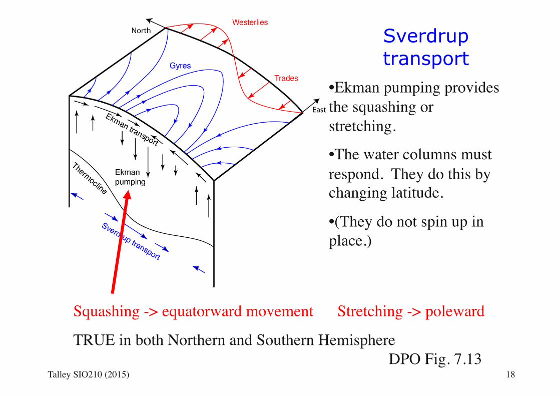
Sverdrup transport

• Ekman pumping provides the squashing or stretching.

• The water columns must respond. They do this by changing latitude.

• (They do not spin up in place.)

Squashing -> equatorward movement Stretching -> poleward

TRUE in both Northern and Southern HemisphereDPO Fig. 7.13

Talley SIO210 (2015) 18

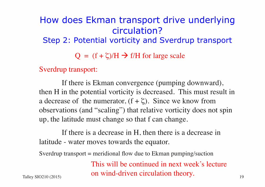
How does Ekman transport drive underlying circulation?

Step 2: Potential vorticity and Sverdrup transport

Q = (f + ζ)/H ! f/H for large scale

Sverdrup transport:

If there is Ekman convergence (pumping downward), then H in the potential vorticity is decreased. This must result in a decrease of the numerator, (f + ζ). Since we know from observations (and “scaling”) that relative vorticity does not spin up, the latitude must change so that f can change.

If there is a decrease in H, then there is a decrease in latitude - water moves towards the equator.Sverdrup transport = meridional flow due to Ekman pumping/suction

Talley SIO210 (2015) 19

This will be continued in next week’s lecture on wind-driven circulation theory.

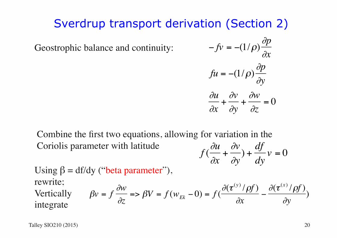
Sverdrup transport derivation (Section 2)

Geostrophic balance and continuity:

€

− fv = −(1/ρ)∂p∂x

fu = −(1/ρ)∂p∂y

∂u∂x

+∂v∂y

+∂w∂z

= 0

Combine the first two equations, allowing for variation in the Coriolis parameter with latitude

€

f (∂u∂x

+∂v∂y) +

dfdyv = 0

Using β = df/dy (“beta parameter”), rewrite;Verticallyintegrate

€

βv = f ∂w∂z

=> βV = f (wEk − 0) = f (∂(τ(y ) /ρf )∂x

−∂(τ (x ) /ρf )

∂y)

Talley SIO210 (2015) 20

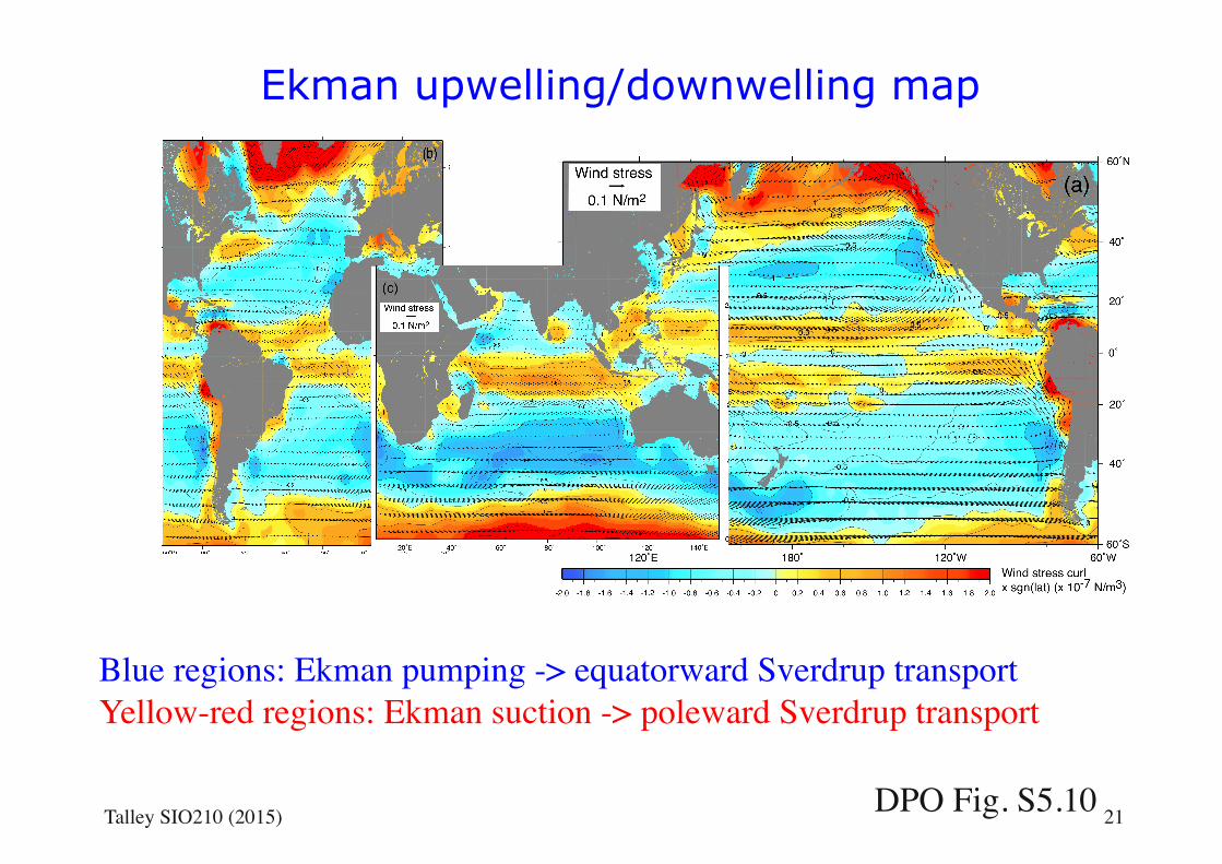
Ekman upwelling/downwelling map

DPO Fig. S5.10

Blue regions: Ekman pumping -> equatorward Sverdrup transportYellow-red regions: Ekman suction -> poleward Sverdrup transport

Talley SIO210 (2015) 21

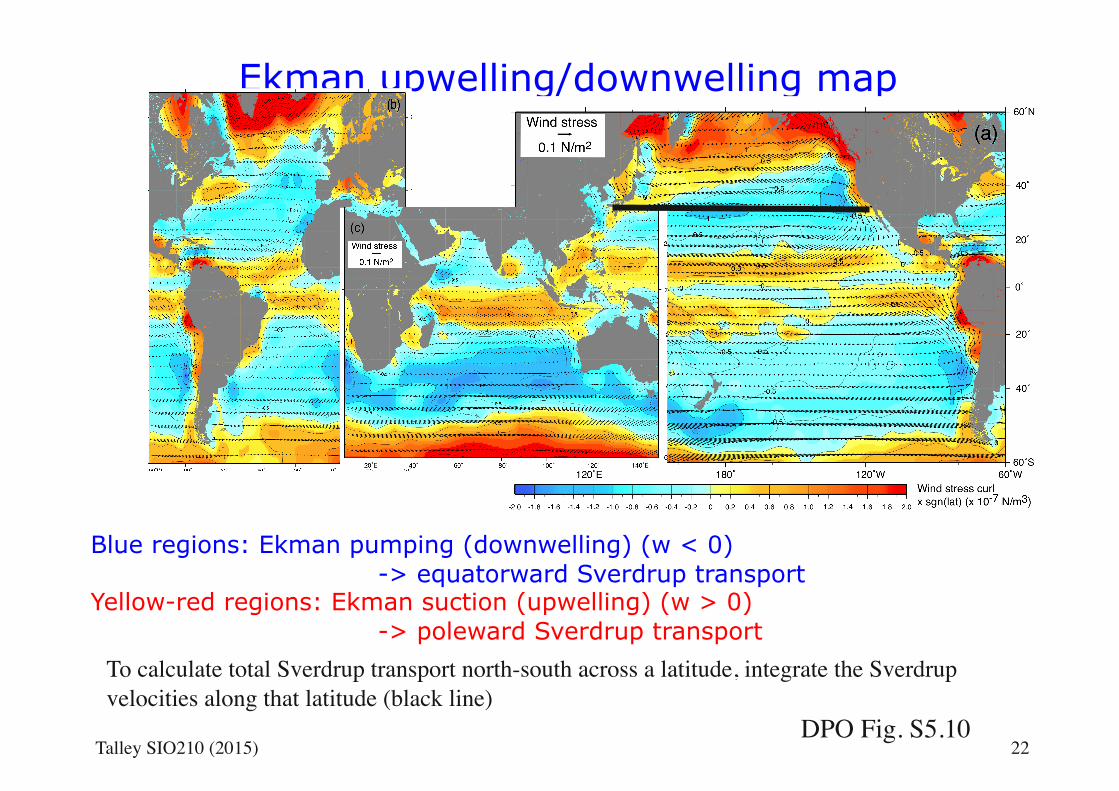
Ekman upwelling/downwelling map

DPO Fig. S5.10

Blue regions: Ekman pumping (downwelling) (w < 0) -> equatorward Sverdrup transport

Yellow-red regions: Ekman suction (upwelling) (w > 0) -> poleward Sverdrup transport

Talley SIO210 (2015) 22

To calculate total Sverdrup transport north-south across a latitude, integrate the Sverdrup velocities along that latitude (black line)

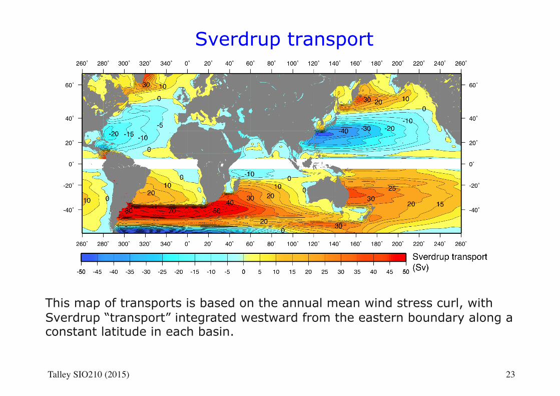
Sverdrup transport DPO Fig. 5.17

This map of transports is based on the annual mean wind stress curl, with Sverdrup “transport” integrated westward from the eastern boundary along a constant latitude in each basin.

Talley SIO210 (2015) 23

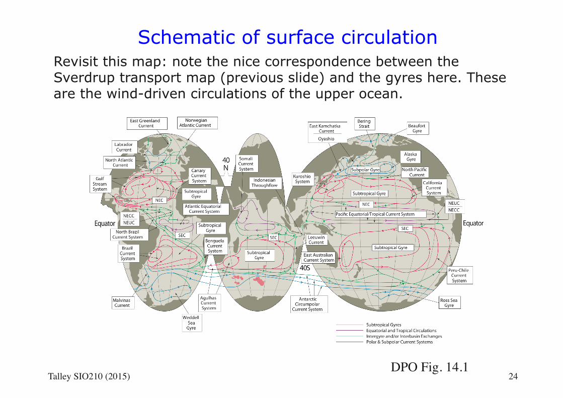
Schematic of surface circulation Revisit this map: note the nice correspondence between the Sverdrup transport map (previous slide) and the gyres here. These are the wind-driven circulations of the upper ocean.

DPO Fig. 14.1Talley SIO210 (2015) 24