Computational Fluid Dynamics JOURNAL 14(4):42 January 2006 (pp.359–378)

SIMULATION OF UNSTEADY TURBULENT FLOWOVER A STALLED AIRFOIL

B. STOCKDILL † G. PEDRO † A. SULEMAN †

F. MAGAGNATO ‡ N. DJILALI †

Abstract

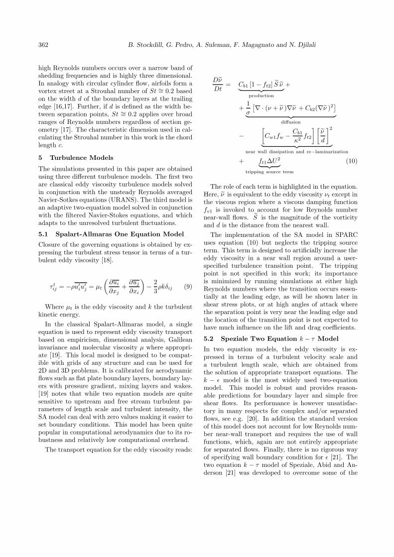
Unsteady, turbulent flow simulations are carried out for a NACA 0012 airfoil. The objective is toassess the performance of various turbulence models for application to fluid-structure interactionand airfoil optimization problems. Unsteady simulations are carried out at an angle of attack of 20degrees and a chord Reynolds number of 105. The Spalart Allmaras and Speziale k− τ models areused in unsteady Reynolds-Averaged Navier-Stokes (URANS) simulations. Filtered Navier Stokessimulations in conjunction with an adaptive k−τ model proposed by Magagnato are also presented.This adaptive model can be used at all grid or temporal resolutions and tends assymptotically toDNS or RANS in the limit of fine grid resolution or steady state simulations. This model producesphysically realistic flow patterns, rich vortex dynamics and non-periodic lift and drag signals. Thek − τ model also yields unsteady flow patterns, but these remain purely periodic, whereas onlysteady state solutions are obtained with the Spalart Allmaras model.Key Words: Unsteady RANS; Turbulence model; Flow separation; Stall

1 INTRODUCTION

Simulation of massively separated flows over an airfoilbeyond stall is, along with prediction of stall itself, avery challenging problem. Panel methods [1]and invis-cid Euler computations, which up until recently havebeen the work horses of aerodynamic design in Indus-try, are unable to predict flow separation and stall,and extensive reliance on wind tunnel measurementsis still required to characterize these flow regimes [2].

These regimes are characterized by unsteadinessand complex turbulence dynamics. Though in princi-ple represented in the Navier-Stokes (NS) equations,the computational resolution of these processes is pro-hibitive for most aerodynamic flows of practical im-portance. The practical limit of a Direct NumericalSimulation (DNS) is Rec = 104, two orders of magni-tude less than an airfoil in the landing configuration[3].

Since designers are primarily interested in the timeaveraged values of shear stress, pressure and veloc-

Received on December 6, 2005.

† Department of Mechanical Engineering, Universityof Victoria; Victoria, BC, V8W 3P6, Canada

‡ Dep. of Fluid Machinery, University of Karlsruhe,Karlsruhe, Germany

ity rather than the time dependent details, practi-cal information and design assessment can often beobtained using the Reynolds Averaged Navier Stokes(RANS) simulations in conjunction with appropriateclosure models to represent the effect of turbulentstresses. Engineering turbulence models, such as theclassical k−ε model, often achieve this via a turbulenteddy viscosity. A weakness common to both eddy-viscosity and Reynolds stress RANS models is the as-sumption that a single time (or length) scale char-acterizes both turbulence transport and dissipationof turbulent kinetic energy, and the energy cascadefrom large to small eddies is not accounted for. Someof these shortcomings can be addressed using multi-ple scale models (e.g. [4]),but it is clear that LargeEddy Simulations (LES) offer a more satisfactory rep-resentation of turbulence transport by resolving mostof the dynamics of the flow and confining turbulencemodelling to unresolved small scale fluctuations only[5].Very encouraging progress has been made in LEScomputations coupled with dynamic subgrid models,but this approach is computationally expensive andis not viable for routine engineering applications, par-ticularly at higher Reynolds numbers. Consequently,intermediate approaches based on Unsteady ReynoldsAveraged Navier-Stokes methods (URANS) as well ashybrid URANS/LES methods [5]are seen as the most

359

360 B. Stockdill, G. Pedro, A. Suleman, F. Magagnato and N. Djilali

viable short and mid-term alternative.Major efforts have been devoted to simulation and

turbulence model validation for airfoil flows near max-imum lift, and an overview of these is provided in thenext Section. In this paper we investigate the abil-ity of three turbulence models to predict massivelyseparated flows and vortex shedding in the post stallregime. Unsteady simulations are presented using twoclassical eddy viscosity models (Spalart Allmaras one-equation, Speziale k − τ two-equation), and a newadaptive turbulence model [7]which has the propertyof adapting to all cell Reynolds numbers and whichreduces the simulations to a DNS in the limit of fullyresolved Kolmogorov scales, and to RANS in the limitof steady state simulations. To keep the computa-tional requirements reasonable, and, in the interest ofpredicting NACA 0012 characteristics at a Reynoldsnumber for which there is little experimental data, theset of simulations is carried out at Rec = 105. The flowover the NACA 0012 airfoil flow remains laminar atlow angles of attack (α < 10◦) for Rec = 105, whereasseparation, Kelvin Helmholtz instabilities, turbulenceand vortex shedding are induced at post stall anglesof attack [8].

2 Overview of CFD Methods for AirfoilAerodynamics

Recent CFD airfoil validation projects include the Eu-ropean Initiative on Validation of CFD Codes (EU-ROVAL), see [9,10]and the European ComputationalAerodynamics Research Project (ECARP). The goalof these projects was to determine the ability of vari-ous turbulence models to predict separation and maxi-mum lift just before stall. Aerospatiale’s A-Airfoil, forwhich there is extensive experimental data, was usedfor validation in both projects. A standard grid with96,512 grid points was used for all simulations. HighReynolds number flow in these conditions is one of themost challenging cases for CFD. ECARP concludedthat algebraic and standard eddy viscosity models failto correctly predict separation and therefore maxi-mum lift at high angles of attack.

Weber and Ducros [10] conducted RANS and LESsimulations over the A-Airfoil near stall at Rec =2.1 × 106. They used the ECARP C type grid with512 points along the airfoil surface, 64 points in thecross stream direction and 498 points in the down-stream direction. They allowed 10 chord lengths tofar field boundaries in the upstream and cross streamdirections. Wall functions were not used; the firstgrid point from the wall was located at approximatelyy+ = 2. While the classic turbulence models were ableto predict many features such as a laminar boundary

layer close to the leading edge, separation at the trail-ing edge and the interaction of two shear layers inthe wake, they failed to correctly predict the separa-tion zone at high angles of attack. Spalart Allmarasmodel results were found to be quantitatively closeto LES, which required 140 times more computer re-sources than the Spalart Allmaras model on the samegrid. Convergence with RANS was however not ob-tained at high angles of attack, and neither RANS norLES were able to predict boundary layer separationwith the correct back flow characteristics.

Chaput [9] carried out validations of turbulencemodels under ECARP using the EUROVAL Aerospa-tiale A-Airfoil grid. Sixteen partners are involved inthe project, including BAe, DLR, Dornier/Dasa-LMand SAAB. The focus is a comparison between theperformance of various turbulence models at maxi-mum lift. The extensive database of numerical andexperimental data from the EUROVAL project is usedas a starting point. The project does not include thealgebraic Baldwin Lomax and the standard k−ε mod-els. While these models are widely used in industry,their widespread failure to predict separation is welldocumented. Examples include Refs.[11,12].

EUROVAL and ECARP found that Navier Stokesmethods are capable of accurate prediction of bound-ary layer separation in pre-stall conditions but thataccurate prediction of maximum lift is not achieved.Good results can be obtained by using turbulencemodels which take into account the strong nonlin-ear equilibrium processes at high angles of attack.Transition to turbulence near the leading edge is stillproblematic; turbulence models do not reliably predicttransition on their own.

trailing edge

x= 0 x= c

x

y

Ufree strea m

α

NAC A 0012

chord

leading edge

Fig.1: Layout of NACA 0012 Airfoil showing Chord,Leading Edge (LE) and Trailing Edge (TE)

3 Definitions

3.1 Airfoil Dimensionless Parameters

The forces which act on an airfoil are functions of den-sity ρ, molecular viscosity μ, free stream velocity U∞and chord length c. Through dimensional analysis,these variables can be combined into a single non-dimensional parameter, the chord Reynolds numberRec which is a measure of the ratio of inertial to vis-

Simulation of Unsteady Turbulent Flow over a Stalled Airfoil 361

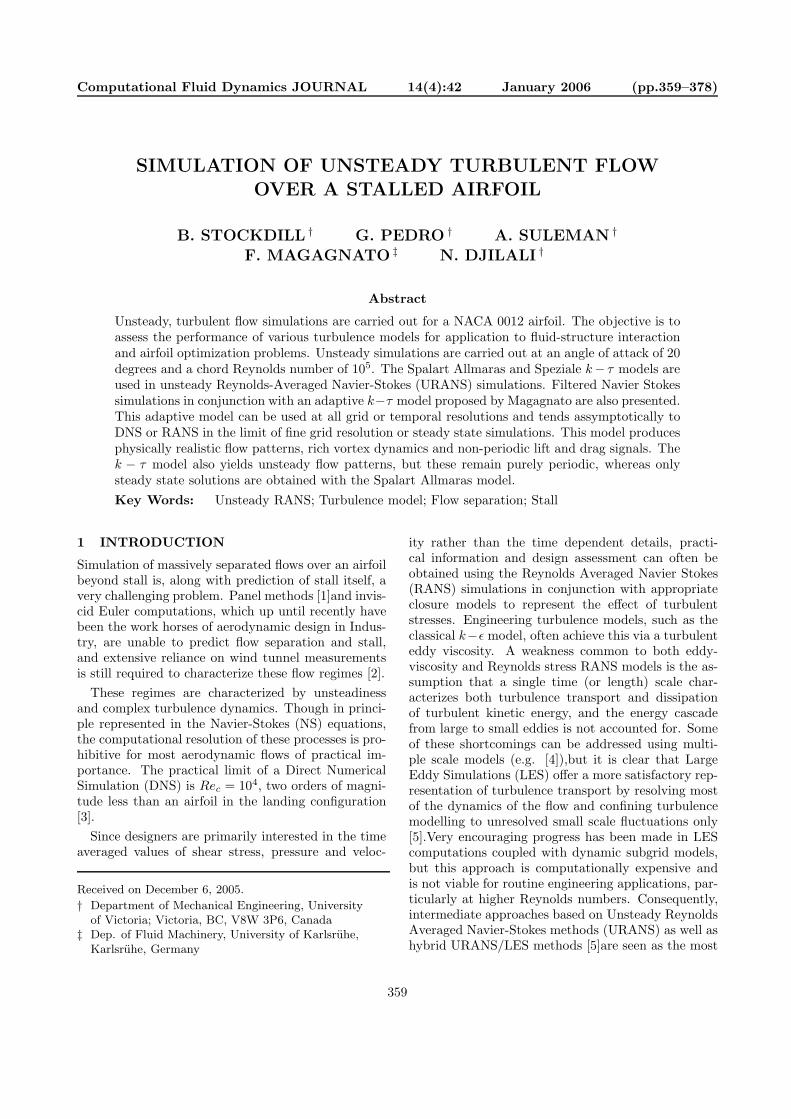
Ufree stream

α

separation bubble

point of separation

NACA 0012

Fig.2: Nomenclature of Flow Separation and Associ-ated Velocity Profiles

cous forces:

Rec =ρU∞c

μ=

U∞c

ν(1)

where ν = μρ is the kinematic viscosity. In analogy

to the Reynolds number, the lift, drag and frictionforces can also be written as non-dimensional coeffi-cients. These are the coefficient of lift Cl, the coeffi-cient of drag Cd, the coefficient of pressure drag Cdp,the coefficient of friction drag Cdf and the skin frictioncoefficient Cf . Forces are non-dimensionalized by thedynamic pressure 1

2 (ρU2∞) and the wing area S. Inthis work S is set to 1 since the simulations are twodimensional.

Cl =lift

12ρU2∞S

(2)

Cd =drag

12ρU2∞S

(3)

Cdf =friction drag

12ρU2∞S

(4)

Cdp =pressure drag

12ρU2∞S

(5)

Cf =shear stress

12ρU2∞

(6)

Pressure forces can also be non-dimensionalized us-ing the difference between the local pressure P , thefree stream pressure P∞ and the dynamic pressure:

Cp =P − P∞12ρU2∞

(7)

Figure 1 shows the geometry of a symmetric NACA0012 airfoil.

• Chord (c): straight line joining the leading andtrailing edges.

• Leading Edge (LE): point at the front of the airfoilwhere the chord line intersects the airfoil surface.

• Trailing Edge (TE): point at the rear of the airfoilwhere the chord line intersects the airfoil surface

• Angle of Attack (α): Angle between the chord lineand the free stream velocity vector U∞.

Only the symmetric (zero camber) NACA 0012 air-foil is used in this work.

4 Vortex Shedding and Stall

It is well established that many structures, particu-larly bluff bodies, shed vortices in subsonic flow [13].Vortex street wakes tend to be very similar regardlessof the body geometry. A well documented example ofvortex shedding is the flow around circular cylinders(see, e.g. [14]). The characteristic non-dimensionalfrequency or Strouhal number St for such flows is de-fined as:

fs =StU∞

L(8)

where fs is the vortex shedding frequency, U∞ thewind speed, and L the characteristic length scale:

Vortex shedding is caused by flow separation, a vis-cous flow phenomenon associated with either abruptchanges in geometry or adverse pressure gradients.There are two main separated flow regimes for theNACA 0012 airfoil. The first corresponds to a lami-nar separation bubble form the leading edge (at aboutCl

∼= 0.9 and α ∼= 9◦ for Rec∼= 3× 106 [15]). The sep-

arated shear layer undergoes transition prior to reat-tachment.

The second separated flow regime corresponds tomassive stall at about α ≈ 16◦; a large separationbubble begins to form at the trailing edge and grad-ually moves forward. This regime is associated withthe shedding of large vortices.

Stall for the NACA 0012 section is difficult to quan-tify experimentally. Gregory and O’Reilly [15] foundthat for Rec

∼= 3 × 106, the stall may originate fromthe collapse of the leading edge laminar separationbubble. However, for higher Rec, the stall appears tooriginate entirely from the forward propagation of thetrailing edge separation bubble.

Whereas vortex shedding for cylinders at lowReynolds numbers in the laminar regime is a station-ary, harmonic two-dimensional phenomenon, this isnot the case for turbulent flow. Vortex shedding at

362 B. Stockdill, G. Pedro, A. Suleman, F. Magagnato and N. Djilali

high Reynolds numbers occurs over a narrow band ofshedding frequencies and is highly three dimensional.In analogy with circular cylinder flow, airfoils form avortex street at a Strouhal number of St ∼= 0.2 basedon the width d of the boundary layers at the trailingedge [16,17]. Further, if d is defined as the width be-tween separation points, St ∼= 0.2 applies over broadranges of Reynolds numbers regardless of section ge-ometry [17]. The characteristic dimension used in cal-culating the Strouhal number in this work is the chordlength c.

5 Turbulence Models

The simulations presented in this paper are obtainedusing three different turbulence models. The first twoare classical eddy viscosity turbulence models solvedin conjunction with the unsteady Reynolds averagedNavier-Sotkes equations (URANS). The third model isan adaptive two-equation model solved in conjunctionwith the filtered Navier-Stokes equations, and whichadapts to the unresolved turbulent fluctuations.

5.1 Spalart-Allmaras One Equation Model

Closure of the governing equations is obtained by ex-pressing the turbulent stress tensor in terms of a tur-bulent eddy viscosity [18].

τ tij = −ρu′

iu′j = μt

(∂ui

∂xj+

∂uj

∂xi

)− 2

3ρkδij (9)

Where μt is the eddy viscosity and k the turbulentkinetic energy.

In the classical Spalart-Allmaras model, a singleequation is used to represent eddy viscosity transportbased on empiricism, dimensional analysis, Galileaninvariance and molecular viscosity μ where appropri-ate [19]. This local model is designed to be compat-ible with grids of any structure and can be used for2D and 3D problems. It is calibrated for aerodynamicflows such as flat plate boundary layers, boundary lay-ers with pressure gradient, mixing layers and wakes.[19] notes that while two equation models are quitesensitive to upstream and free stream turbulent pa-rameters of length scale and turbulent intensity, theSA model can deal with zero values making it easier toset boundary conditions. This model has been quitepopular in computational aerodynamics due to its ro-bustness and relatively low computational overhead.

The transport equation for the eddy viscosity reads:

Dν

Dt= Cb1 [1 − ft2] S ν︸ ︷︷ ︸

production

+

+1σ

[∇ · (ν + ν )∇ν + Cb2(∇ν )2]

︸ ︷︷ ︸diffusion

−[Cw1fw − Cb1

κ2ft2

] [ν

d

]2

︸ ︷︷ ︸near wall dissipation and re−laminarization

+ ft1ΔU2︸ ︷︷ ︸tripping source term

(10)

The role of each term is highlighted in the equation.Here, ν is equivalent to the eddy viscosity νt except inthe viscous region where a viscous damping functionfv1 is invoked to account for low Reynolds numbernear-wall flows. S is the magnitude of the vorticityand d is the distance from the nearest wall.

The implementation of the SA model in SPARCuses equation (10) but neglects the tripping sourceterm. This term is designed to artificially increase theeddy viscosity in a near wall region around a user-specified turbulence transition point. The trippingpoint is not specified in this work; its importanceis minimized by running simulations at either highReynolds numbers where the transition occurs essen-tially at the leading edge, as will be shown later inshear stress plots, or at high angles of attack wherethe separation point is very near the leading edge andthe location of the transition point is not expected tohave much influence on the lift and drag coefficients.

5.2 Speziale Two Equation k − τ Model

In two equation models, the eddy viscosity is ex-pressed in terms of a turbulent velocity scale anda turbulent length scale, which are obtained fromthe solution of appropriate transport equations. Thek − ε model is the most widely used two-equationmodel. This model is robust and provides reason-able predictions for boundary layer and simple freeshear flows. Its performance is however unsatisfac-tory in many respects for complex and/or separatedflows, see e.g. [20]. In addition the standard versionof this model does not account for low Reynolds num-ber near-wall transport and requires the use of wallfunctions, which, again are not entirely appropriatefor separated flows. Finally, there is no rigorous wayof specifying wall boundary condition for ε [21]. Thetwo equation k − τ model of Speziale, Abid and An-derson [21] was developed to overcome some of the

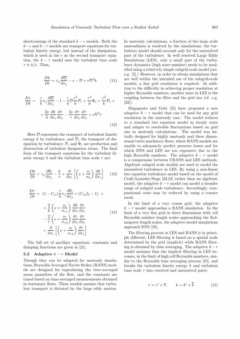
Simulation of Unsteady Turbulent Flow over a Stalled Airfoil 363

shortcomings of the standard k − ε models. Both thek−ε and k−τ models use transport equations for tur-bulent kinetic energy, but instead of the dissipation,which is used in the ε as the second transport equa-tion, the k − τ model uses the turbulent time scaleτ ≡ k/ε. Thus,

Dk

Dt= τij

∂ui

∂xj− ε −D + ν∇2k (11)

Dτ

Dt=

τ

kτij

∂ui

∂xj− 1 − τ

kD τ2

kPε +

τ2

kΦε +

τ2

kDε +

+2ν

k

∂k

∂xi

∂τ

∂xi− 2ν

τ

∂τ

∂xi

∂τ

∂xi+ ν∇2τ

(12)

Here D represents the transport of turbulent kineticenergy k by turbulence, and Dε the transport of dis-sipation by turbulence; Pε and Φε are production anddestruction of turbulent dissipation terms. The finalform of the transport equations for the turbulent ki-netic energy k and the turbulent time scale τ are:

Dk

Dt= τij

∂ui

∂xj− k

τ+

∂

∂xi

[(ν +

νt

σk

)∂k

∂xi

](13)

Dτ

Dt= (1 − Cε1)

τ

kτij

∂ui

∂xj+ (Cε2f2 − 1) +

+2k

(ν +

νt

στ1

)∂k

∂xi

∂τ

∂xi

− 2τ

(ν +

νt

στ2

)∂τ

∂xi

∂τ

∂xi

+∂

∂xi

[(ν +

νt

στ2

)∂τ

∂xi

](14)

The full set of ancillary equations, constants anddamping functions are given in [21].

5.3 Adaptive k − τ Model

Though they can be adapted for unsteady simula-tions, Reynolds Averaged Navier Stokes (RANS) mod-els are designed for reproducing the time-averagedmean quantities of the flow, and the constants aretuned based on time-averaged measurements obtainedin stationary flows. These models assume that turbu-lent transport is dictated by the large eddy motion.

In unsteady calculations, a fraction of the large scaleunsteadiness is resolved by the simulations; the tur-bulence model should account only for the unresolvedpart of the turbulence. In well resolved Large EddySimulations (LES), only a small part of the turbu-lence dynamics (high wave number) needs to be mod-elled using a relatively simple subgrid scale model (see.e.g. [5].) However, in order to obtain simulations thatare well within the intended use of the subgrid-scalemodels, a fine grid resolution is required. In addi-tion to the difficulty in achieving proper resolution athigher Reynolds numbers, another issue in LES is thecoupling between the filter and the grid size (cf. e.g.[22]).

Magagnato and Gabi [25] have proposed a newadaptive k − τ model that can be used for any gridresolution in the unsteady case. The model reducesto a standard two equation model in steady stateand adapts to resolvable fluctuations based on gridsize in unsteady calculations. The model was ini-tially designed for highly unsteady and three dimen-sional turbo machinery flows, where RANS models areunable to adequately predict pressure losses and forwhich DNS and LES are too expensive due to thehigh Reynolds numbers. The adaptive k − τ modelis a compromise between URANS and LES methods.Algebraic subgrid scale models are used to model theunresolved turbulence in LES. By using a non-lineartwo equation turbulence model based on the model ofCraft/Launder/Suga [23,24] rather than an algebraicmodel, the adaptive k− τ model can model a broaderrange of subgrid scale turbulence. Accordingly, com-puational costs may be reduced by using a coarsermesh.

In the limit of a very coarse grid, the adaptivek − τ model approaches a RANS simulation. In thelimit of a very fine grid in three dimensions with cellReynolds number length scales approaching the Kol-mogorov length scales, the adaptive model simulationsapproach DNS [25].

The filtering process in LES and RANS is in princi-ple different; LES filtering is based on a spatial scaledetermined by the grid (implicit) while RANS filter-ing is obtained by time averaging. The adaptive k− τmodel assumes that the implicit filtering in LES be-comes, in the limit of high cell Reynolds numbers, sim-ilar to the Reynolds time averaging process [25], andbreaks the turbulent kinetic energy k and turbulenttime scale τ into resolved and unresolved parts:

τ = τ ′ + τ, k = k′ + k (15)

364 B. Stockdill, G. Pedro, A. Suleman, F. Magagnato and N. Djilali

The resolved part of the turbulent kinetic energy kis obtained as part of the numerical solution. The un-resolved part k′ is modelled with an additional trans-port equation. The resolved time scale is obtained aposteriori using a model for isotropic high Reynoldsnumber flows where τ is determined by the unresolvedturbulent kinetic energy k′ and the filter length scaleLΔ:

τ =LΔ√

k′ (16)

The filter length scale (LΔ) is determined by takingthe maximum of the grid length scale (LS) and thetime step or temporal length scale (Lt):

LS = 2 ·√

Δx · Δy · Δz, Lt = |u| · Δt (17)

LΔ = max(LS , Lt) (18)

The subgrid scale stresses are obtained as follows:

−ρu′iu

′j = ρcμk′τ ′Sij − 2

3ρk′δij − ρv′iv

′j +

23ρk′δij

(19)

where v′i are random velocities estimated at eachtime step using a Langevin-type equation. An impor-tant feature of the adaptive model is that it accountsfor backscatter (second half of the RHS of equation19).

The transport equations for the unresolved turbu-lent kinetic energy k′ and time scale τ ′ are obtainedby recasting the model of [23]. Further details on theadaptive model can be found in [25].

6 Computational Procedure

The research code SPARC (Structured PArallelResearch Code) developed at the University ofKarlsruhe, Germany [25]. is used in this study. Themodular structure of SPARC is particularly suited tomulti-team developments and collaboration, and thecode is being integrated into a fluid-structure interac-tion framework at UVic.

SPARC is a finite-volume, structured, parallelmulti-block code. In the simulations presented here,the full compressible form of the RANS equations aresolved for the Spalart Allmaras and Speziale k−τ tur-bulence models [26], and the full weakly compressible

Navier Stokes equations with implicit filtering set bythe grid resolution are solved for the adaptive k − τmodel. A two stage semi-discrete method process isused. The first stage is a central difference (cell cen-tered) finite volume discretization in space, and thesecond stage is an explicit Runge-Kutta discretizationin time. The space discretization reduces the partialdifferential equations to a set of ordinary differentialequations continuous in time.

A numerical dissipation term is introduced in thecentral differencing scheme to account for high fre-quency cascading. The dissipation term is a blend ofsecond and fourth order differences where the secondorder differences are designed to prevent spurious os-cillations, particularly around shocks in compressibleflow, and the fourth order terms are designed to im-prove stability and steady state convergence [25].

An efficient full multigrid solver with implicit aver-aging technique is used. The multigrid implementa-tion in SPARC has been found to yield up to tenfoldconvergence acceleration [25].

7 Simulation Results

Prior to discussing the results it should be noted thatthe choice of Rec = 3 × 105 for the simulations wasdictated by computational costs as well as a focus forthe eventual application of this work to investigatelow-intermediate Reynolds number fluid-structure in-teraction problems in flapping propulsion [14] and forsmall aerial vehicles such as gliders and very high alti-tude aircraft (greater than 30,000 m) operating in thisregime [27,28]. Also low Reynolds number airfoil datais of interest since little experimental data is availableat Rec = 105, particularly in stall conditions.

For the NACA 0012 airfoil at low angles of attack(α < 10◦) there is no appreciable separation of themean flow and the time averaged shear stress at everypoint on the airfoil surface is positive. There are ofcourse small scale velocity fluctuations in the turbu-lent boundary layer and some negative instantaneousvelocities, but their time average remains positive.

As the angle of attack increases above 13◦, the ad-verse pressure gradient on the upper side of the airfoilleads to flow separation. The mean velocity close tothe wall becomes negative in certain locations. Largevortices whose diameters are similar in scale to thechord length are shed; there is significant variation inthe coefficients of lift (Cl) and drag (Cd) with time.The physics of such separated flows become muchmore complex and are therefore much more challeng-ing for the turbulence models [12,29].

Since the Reynolds number is Rec = 105, the mesh

Simulation of Unsteady Turbulent Flow over a Stalled Airfoil 365

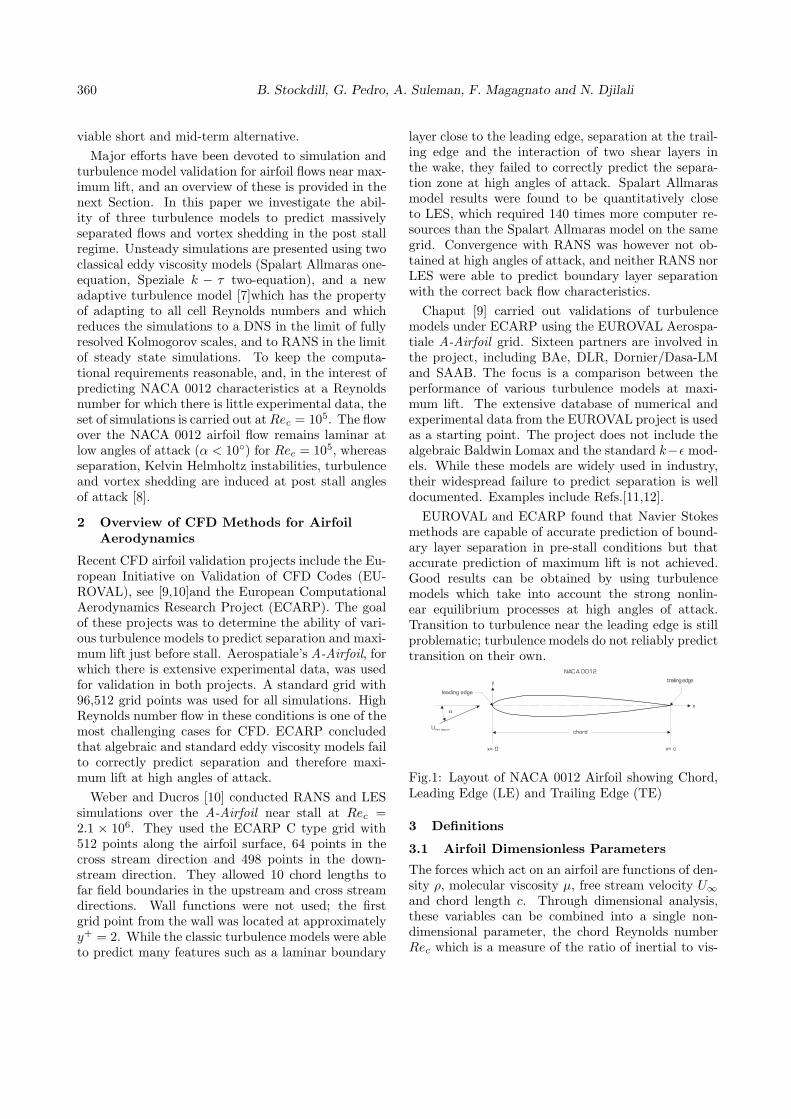
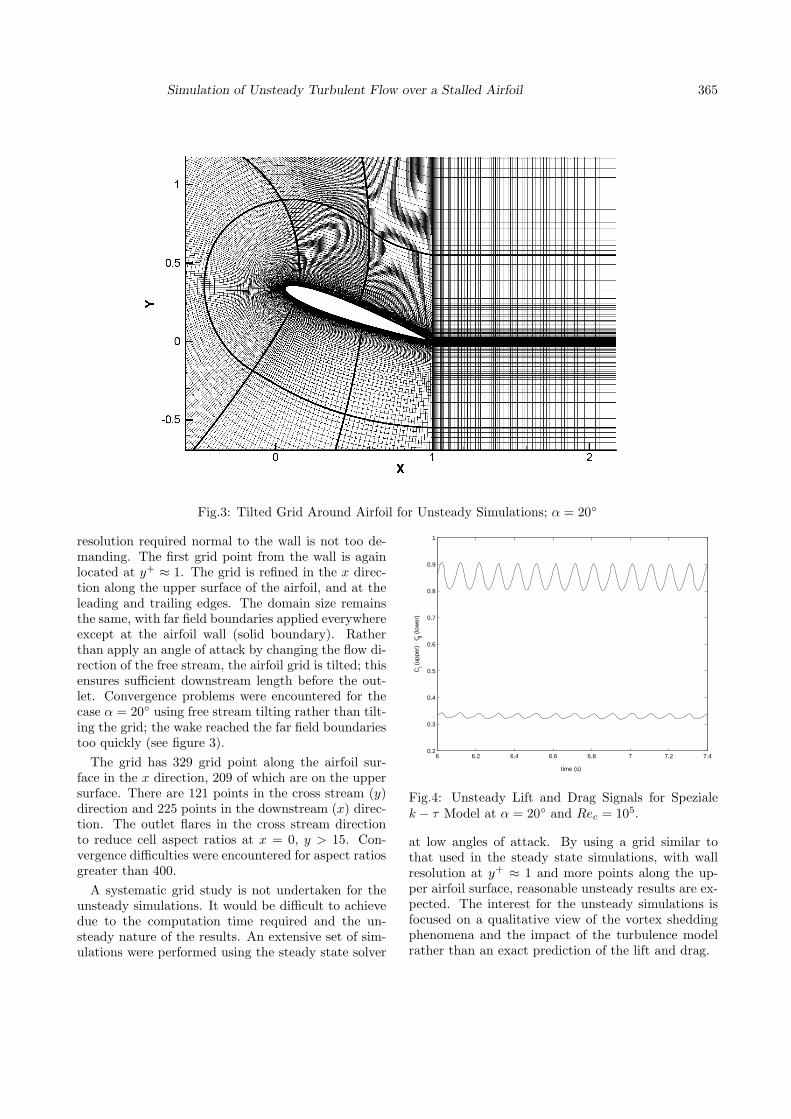
Fig.3: Tilted Grid Around Airfoil for Unsteady Simulations; α = 20◦

resolution required normal to the wall is not too de-manding. The first grid point from the wall is againlocated at y+ ≈ 1. The grid is refined in the x direc-tion along the upper surface of the airfoil, and at theleading and trailing edges. The domain size remainsthe same, with far field boundaries applied everywhereexcept at the airfoil wall (solid boundary). Ratherthan apply an angle of attack by changing the flow di-rection of the free stream, the airfoil grid is tilted; thisensures sufficient downstream length before the out-let. Convergence problems were encountered for thecase α = 20◦ using free stream tilting rather than tilt-ing the grid; the wake reached the far field boundariestoo quickly (see figure 3).

The grid has 329 grid point along the airfoil sur-face in the x direction, 209 of which are on the uppersurface. There are 121 points in the cross stream (y)direction and 225 points in the downstream (x) direc-tion. The outlet flares in the cross stream directionto reduce cell aspect ratios at x = 0, y > 15. Con-vergence difficulties were encountered for aspect ratiosgreater than 400.

A systematic grid study is not undertaken for theunsteady simulations. It would be difficult to achievedue to the computation time required and the un-steady nature of the results. An extensive set of sim-ulations were performed using the steady state solver

6 6.2 6.4 6.6 6.8 7 7.2 7.40.2

0.3

0.4

0.5

0.6

0.7

0.8

0.9

1

time (s)

Cl (

uppe

r)

C d (lo

wer

)

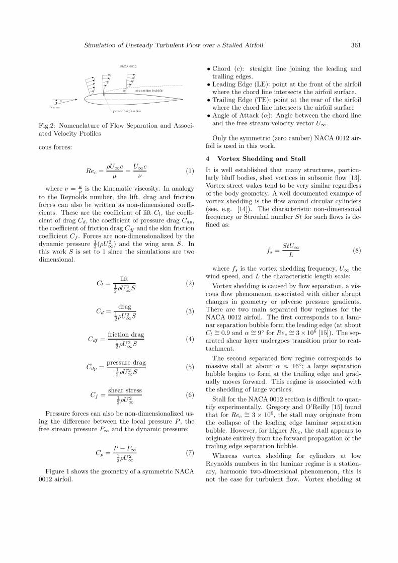
Fig.4: Unsteady Lift and Drag Signals for Spezialek − τ Model at α = 20◦ and Rec = 105.

at low angles of attack. By using a grid similar tothat used in the steady state simulations, with wallresolution at y+ ≈ 1 and more points along the up-per airfoil surface, reasonable unsteady results are ex-pected. The interest for the unsteady simulations isfocused on a qualitative view of the vortex sheddingphenomena and the impact of the turbulence modelrather than an exact prediction of the lift and drag.

366 B. Stockdill, G. Pedro, A. Suleman, F. Magagnato and N. Djilali

7.1 Spalart Allmaras

The Spalart Allmaras model did not produce an un-steady flow pattern at α = 0◦ and Rec = 105 withthe free stream eddy viscosity set to 1. At a lowfree stream eddy viscosity of 10−6, oscillations werepresent in the lift and drag signals but there were largeeddy viscosity gradients near the domain boundaries.It was not possible to converge the solution at eachtime step. To overcome the problems at the bound-aries and to stabilize the solution, the eddy viscositywas set to 1. For the sake of consistency, this matchesthe boundary conditions applied to the adaptive k− τand Speziale k−τ models. It should also be noted thatthe Spalart Allmaras model implemented in SPARChas been tuned for steady state solutions; it appearsthat applying it to unsteady problem would requireat least adjustment of the model constants to avoidexcessive damping. The poor ability of this model incapturing the dynamics of recirculating flows was alsonoted recently by [6]. To allow comparison, contourplots of the Spalart Allmaras results at α = 20◦ andRec = 105 are presented with time averaged resultsfor the Speziale k − τ and adaptive k − τ models.

7.2 Speziale k − τ

Figure 4 shows the lift and drag signals for the KTSmodel at Rec = 105 and α = 20◦. The frequencyand phase of the lift and drag are identical; the signalis periodic. The period is approximately 0.1 secondswhich corresponds to a Strouhal number of St = 0.55based on the chord length c, the free stream veloc-ity U∞ = 18.125m/s and the shedding frequency.The mean values of the lift and drag coefficients areCl ≈ 0.85 and Cd ≈ 0.33. The time step for thesecomputations is 0.005 seconds; this corresponds to 20time steps per shedding cycle.

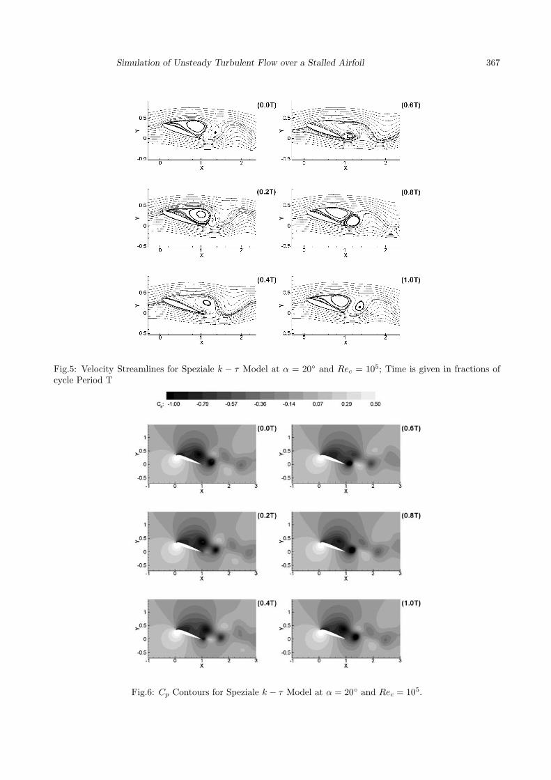
Streamlines for the vortex shedding cycle are shownin Figure 5 with time increments of 0.2T where T isthe cycle period. The large separated clockwise ro-tating vortex in the 0T frame gradually moves down-stream. It detaches from the airfoil at approximately0.4T . Note that a counterclockwise rotating vorteximmediately downstream of the clockwise rotating onehas already separated. At 0.6T a counterclockwise ro-tating trailing edge vortex edge appears. It is shed at0.8T and a clockwise rotating vortex is re-establishedat the leading edge. Two vortices are shed in eachcycle, one generated at the leading edge and the otherat the trailing edge.

Figure 6 shows the pressure contours. Note thatthere is a low pressure region at the centre of eachvortex.

9 9.2 9.4 9.6 9.8 10 10.2 10.4 10.6 10.8 110.2

0.4

0.6

0.8

1

1.2

1.4

1.6

1.8

time (s)

Cl (

uppe

r)

Cd (

low

er)

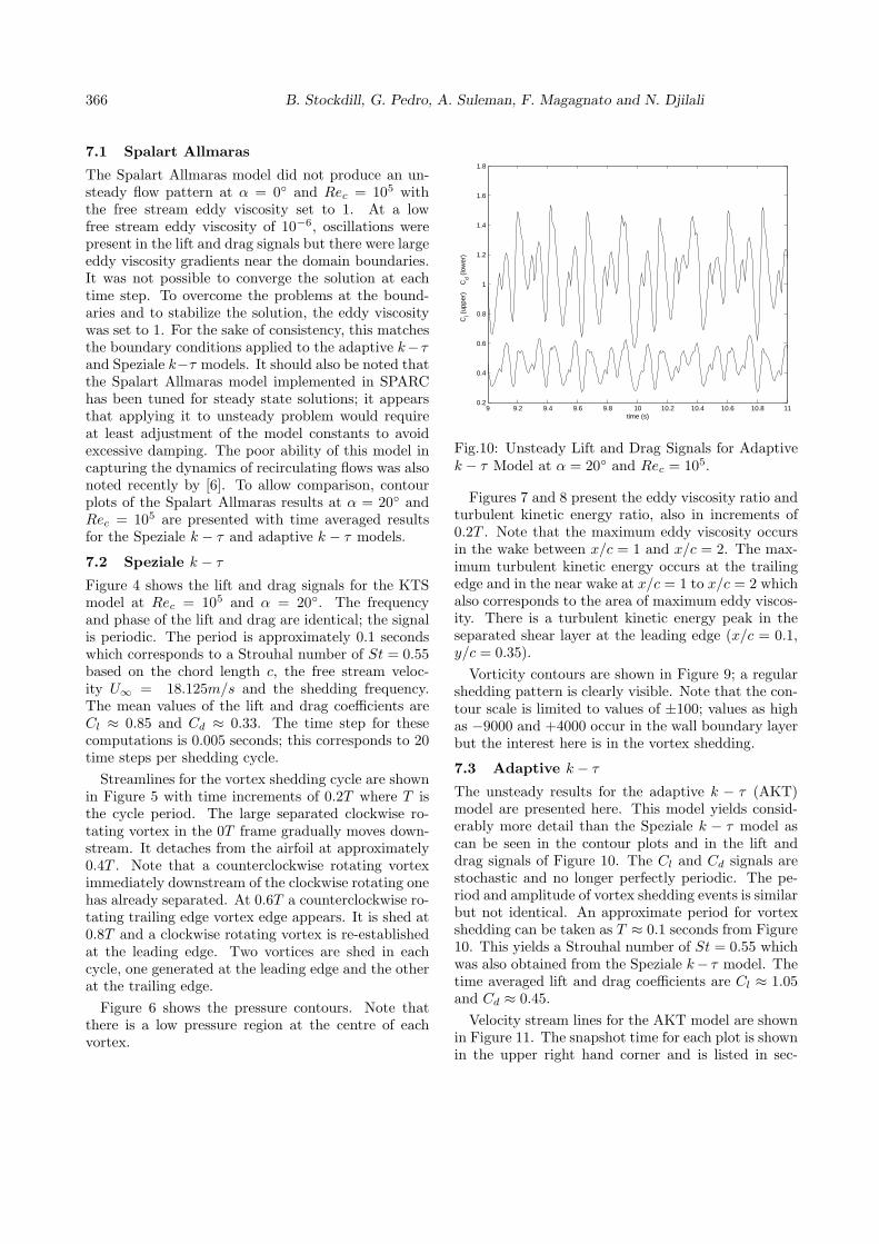
Fig.10: Unsteady Lift and Drag Signals for Adaptivek − τ Model at α = 20◦ and Rec = 105.

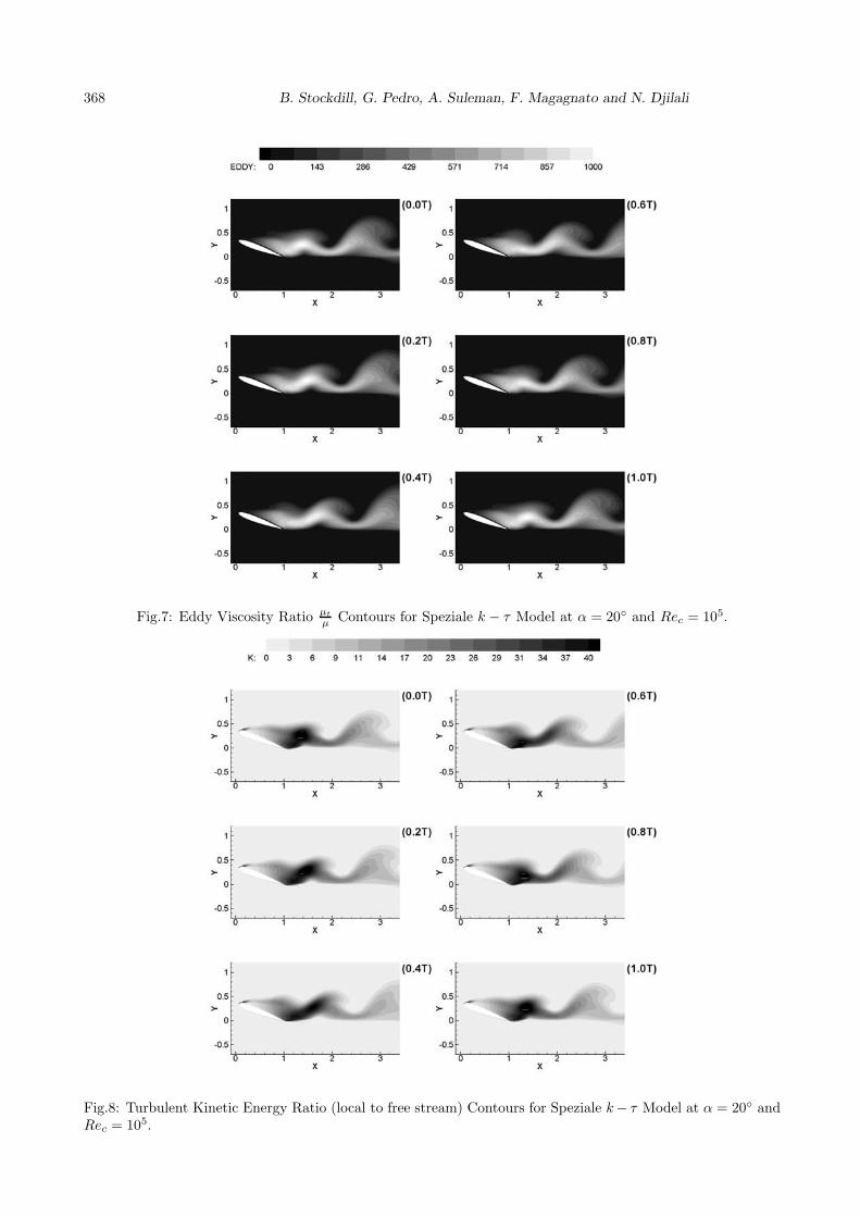
Figures 7 and 8 present the eddy viscosity ratio andturbulent kinetic energy ratio, also in increments of0.2T . Note that the maximum eddy viscosity occursin the wake between x/c = 1 and x/c = 2. The max-imum turbulent kinetic energy occurs at the trailingedge and in the near wake at x/c = 1 to x/c = 2 whichalso corresponds to the area of maximum eddy viscos-ity. There is a turbulent kinetic energy peak in theseparated shear layer at the leading edge (x/c = 0.1,y/c = 0.35).

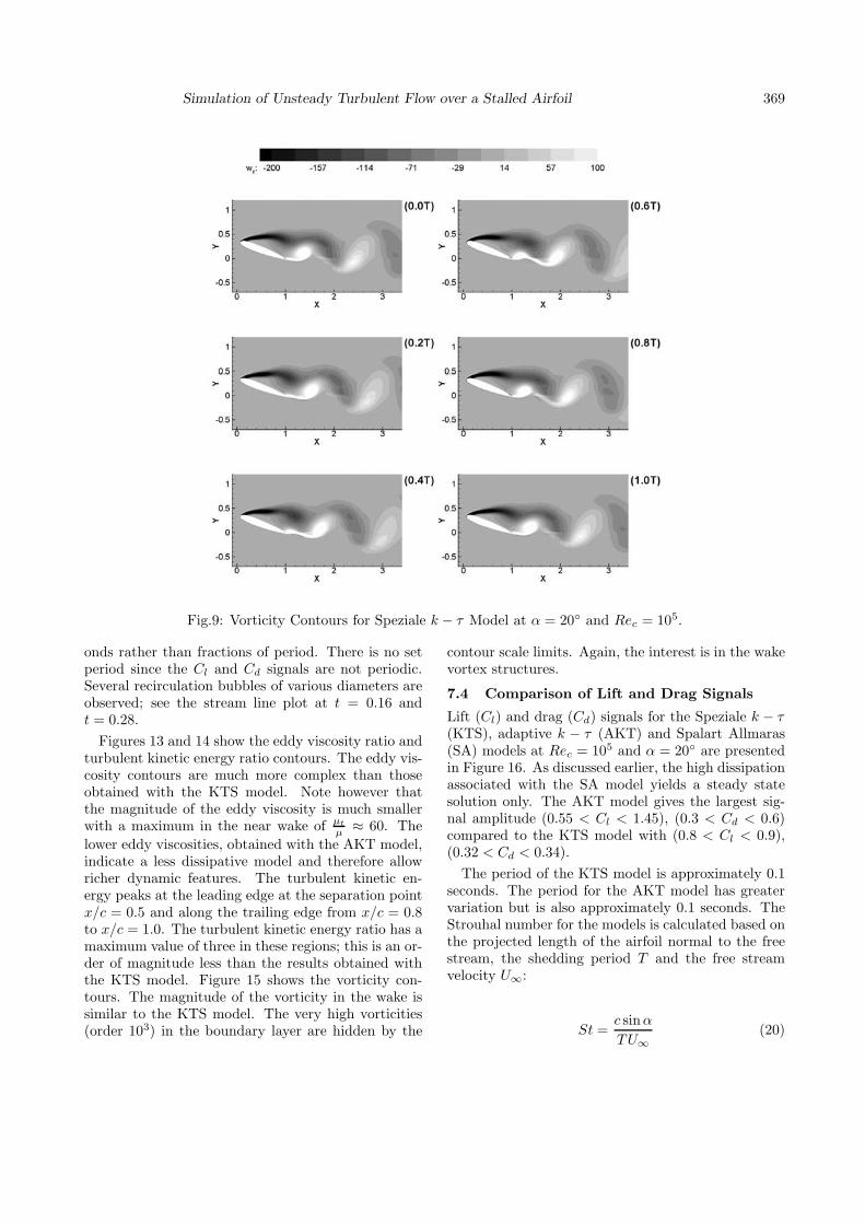
Vorticity contours are shown in Figure 9; a regularshedding pattern is clearly visible. Note that the con-tour scale is limited to values of ±100; values as highas −9000 and +4000 occur in the wall boundary layerbut the interest here is in the vortex shedding.

7.3 Adaptive k − τ

The unsteady results for the adaptive k − τ (AKT)model are presented here. This model yields consid-erably more detail than the Speziale k − τ model ascan be seen in the contour plots and in the lift anddrag signals of Figure 10. The Cl and Cd signals arestochastic and no longer perfectly periodic. The pe-riod and amplitude of vortex shedding events is similarbut not identical. An approximate period for vortexshedding can be taken as T ≈ 0.1 seconds from Figure10. This yields a Strouhal number of St = 0.55 whichwas also obtained from the Speziale k− τ model. Thetime averaged lift and drag coefficients are Cl ≈ 1.05and Cd ≈ 0.45.

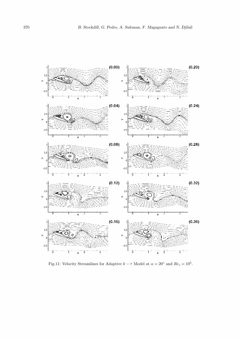
Velocity stream lines for the AKT model are shownin Figure 11. The snapshot time for each plot is shownin the upper right hand corner and is listed in sec-

Simulation of Unsteady Turbulent Flow over a Stalled Airfoil 367

Fig.5: Velocity Streamlines for Speziale k − τ Model at α = 20◦ and Rec = 105; Time is given in fractions ofcycle Period T

Fig.6: Cp Contours for Speziale k − τ Model at α = 20◦ and Rec = 105.

368 B. Stockdill, G. Pedro, A. Suleman, F. Magagnato and N. Djilali

Fig.7: Eddy Viscosity Ratio μt

μ Contours for Speziale k − τ Model at α = 20◦ and Rec = 105.

Fig.8: Turbulent Kinetic Energy Ratio (local to free stream) Contours for Speziale k− τ Model at α = 20◦ andRec = 105.

Simulation of Unsteady Turbulent Flow over a Stalled Airfoil 369

Fig.9: Vorticity Contours for Speziale k − τ Model at α = 20◦ and Rec = 105.

onds rather than fractions of period. There is no setperiod since the Cl and Cd signals are not periodic.Several recirculation bubbles of various diameters areobserved; see the stream line plot at t = 0.16 andt = 0.28.

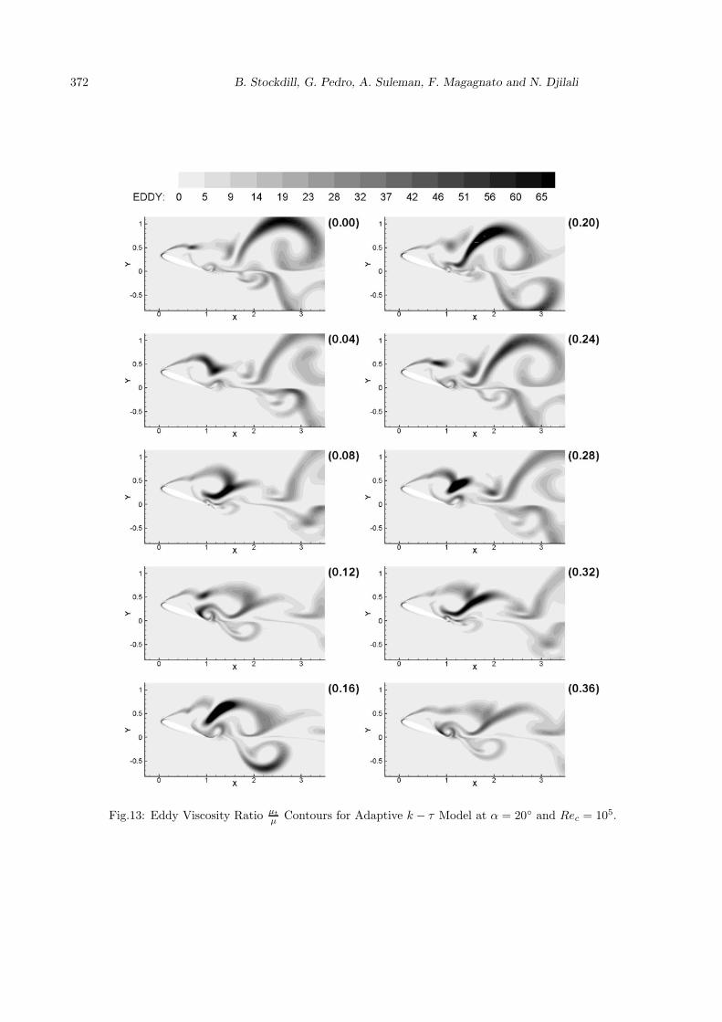
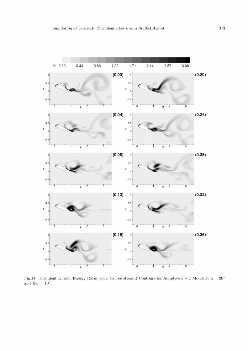
Figures 13 and 14 show the eddy viscosity ratio andturbulent kinetic energy ratio contours. The eddy vis-cosity contours are much more complex than thoseobtained with the KTS model. Note however thatthe magnitude of the eddy viscosity is much smallerwith a maximum in the near wake of μt

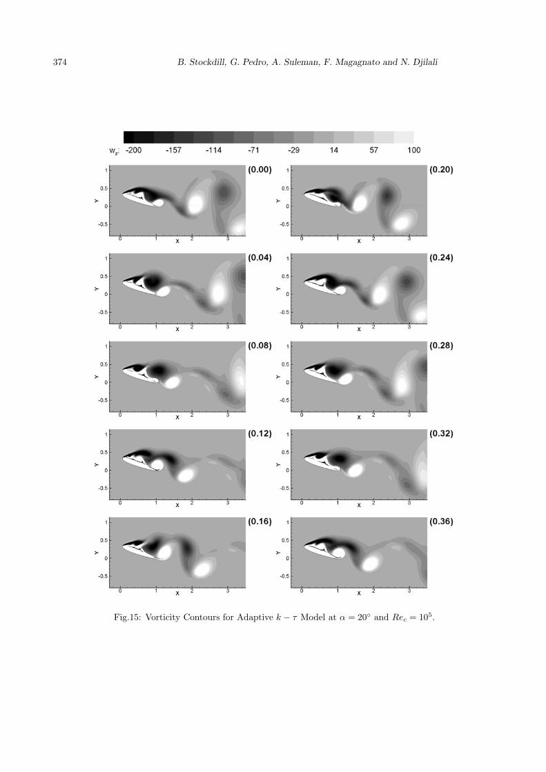
μ ≈ 60. Thelower eddy viscosities, obtained with the AKT model,indicate a less dissipative model and therefore allowricher dynamic features. The turbulent kinetic en-ergy peaks at the leading edge at the separation pointx/c = 0.5 and along the trailing edge from x/c = 0.8to x/c = 1.0. The turbulent kinetic energy ratio has amaximum value of three in these regions; this is an or-der of magnitude less than the results obtained withthe KTS model. Figure 15 shows the vorticity con-tours. The magnitude of the vorticity in the wake issimilar to the KTS model. The very high vorticities(order 103) in the boundary layer are hidden by the

contour scale limits. Again, the interest is in the wakevortex structures.

7.4 Comparison of Lift and Drag Signals

Lift (Cl) and drag (Cd) signals for the Speziale k − τ(KTS), adaptive k − τ (AKT) and Spalart Allmaras(SA) models at Rec = 105 and α = 20◦ are presentedin Figure 16. As discussed earlier, the high dissipationassociated with the SA model yields a steady statesolution only. The AKT model gives the largest sig-nal amplitude (0.55 < Cl < 1.45), (0.3 < Cd < 0.6)compared to the KTS model with (0.8 < Cl < 0.9),(0.32 < Cd < 0.34).

The period of the KTS model is approximately 0.1seconds. The period for the AKT model has greatervariation but is also approximately 0.1 seconds. TheStrouhal number for the models is calculated based onthe projected length of the airfoil normal to the freestream, the shedding period T and the free streamvelocity U∞:

St =c sinα

TU∞(20)

370 B. Stockdill, G. Pedro, A. Suleman, F. Magagnato and N. Djilali

Fig.11: Velocity Streamlines for Adaptive k − τ Model at α = 20◦ and Rec = 105.

Simulation of Unsteady Turbulent Flow over a Stalled Airfoil 371

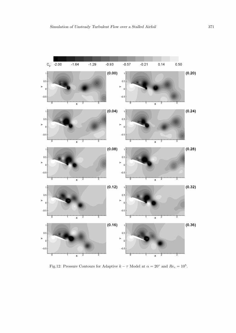
Fig.12: Pressure Contours for Adaptive k − τ Model at α = 20◦ and Rec = 105.

372 B. Stockdill, G. Pedro, A. Suleman, F. Magagnato and N. Djilali

Fig.13: Eddy Viscosity Ratio μt

μ Contours for Adaptive k − τ Model at α = 20◦ and Rec = 105.

Simulation of Unsteady Turbulent Flow over a Stalled Airfoil 373

Fig.14: Turbulent Kinetic Energy Ratio (local to free stream) Contours for Adaptive k − τ Model at α = 20◦

and Rec = 105.

374 B. Stockdill, G. Pedro, A. Suleman, F. Magagnato and N. Djilali

Fig.15: Vorticity Contours for Adaptive k − τ Model at α = 20◦ and Rec = 105.

Simulation of Unsteady Turbulent Flow over a Stalled Airfoil 375

6 6.1 6.2 6.3 6.4 6.5 6.6 6.7 6.8 6.9 70.5

0.6

0.7

0.8

0.9

1

1.1

1.2

1.3

1.4

1.5

time (s)

Cl

Spalart AllmarasSpeziale K−τAdaptive K−τ

Fig.16: Comparison of Unsteady Lift Signals forSpalart Allmaras, Speziale k − τ and Adaptive k − τmodels at α = 20◦ and Rec = 105.

6 6.1 6.2 6.3 6.4 6.5 6.6 6.7 6.8 6.9 70.2

0.3

0.4

0.5

0.6

0.7

time (s)

Cd

Spalart AllmarasSpeziale k−τAdaptive k−τ

Fig.17: Comparison of Unsteady Drag Signals forSpalart Allmaras, Speziale k − τ and Adaptive k − τmodels at α = 20◦ and Rec = 105.

This yields a Strouhal number of 0.19 for the KTSmodel and 0.17 for the AKT model. Experimentally,bluff bodies, including airfoils at high angles of attack,have Strouhal numbers of approximately 0.21; this isslightly higher than predicted here.

7.5 Comparison of Time Averaged ContourPlots

Plots of the time averaged streamlines, velocity, pres-sure, eddy viscosity, turbulent time scale and turbu-lent kinetic energy are presented. Averaging was doneover 2000 time steps; this removes the effect of thestarting and stopping points in the vortex shedding

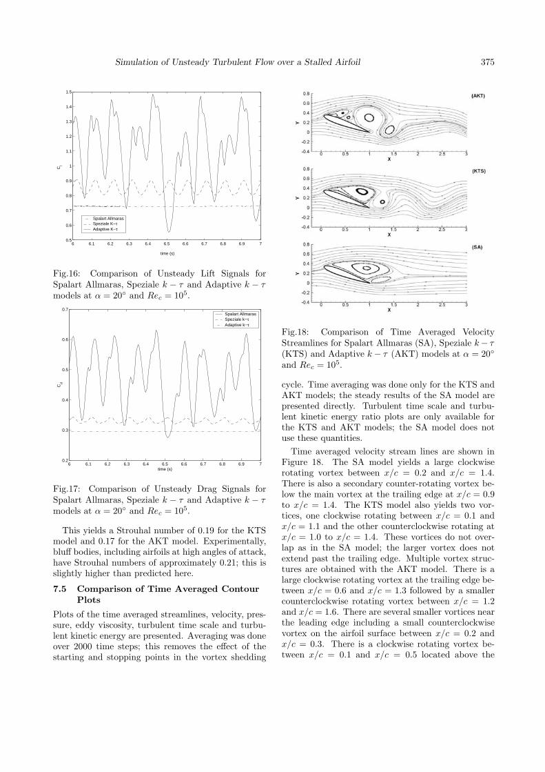
Fig.18: Comparison of Time Averaged VelocityStreamlines for Spalart Allmaras (SA), Speziale k− τ(KTS) and Adaptive k − τ (AKT) models at α = 20◦

and Rec = 105.

cycle. Time averaging was done only for the KTS andAKT models; the steady results of the SA model arepresented directly. Turbulent time scale and turbu-lent kinetic energy ratio plots are only available forthe KTS and AKT models; the SA model does notuse these quantities.

Time averaged velocity stream lines are shown inFigure 18. The SA model yields a large clockwiserotating vortex between x/c = 0.2 and x/c = 1.4.There is also a secondary counter-rotating vortex be-low the main vortex at the trailing edge at x/c = 0.9to x/c = 1.4. The KTS model also yields two vor-tices, one clockwise rotating between x/c = 0.1 andx/c = 1.1 and the other counterclockwise rotating atx/c = 1.0 to x/c = 1.4. These vortices do not over-lap as in the SA model; the larger vortex does notextend past the trailing edge. Multiple vortex struc-tures are obtained with the AKT model. There is alarge clockwise rotating vortex at the trailing edge be-tween x/c = 0.6 and x/c = 1.3 followed by a smallercounterclockwise rotating vortex between x/c = 1.2and x/c = 1.6. There are several smaller vortices nearthe leading edge including a small counterclockwisevortex on the airfoil surface between x/c = 0.2 andx/c = 0.3. There is a clockwise rotating vortex be-tween x/c = 0.1 and x/c = 0.5 located above the

376 B. Stockdill, G. Pedro, A. Suleman, F. Magagnato and N. Djilali

Fig.19: Comparison of Time Averaged U/U∞ Velocityfor Spalart Allmaras (SA), Speziale k − τ (KTS) andAdaptive k − τ (AKT) models at α = 20◦ and Rec =105.

surface vortex, and another counterclockwise rotatingvortex downstream of it from x/c = 0.4 to x/c = 0.7.

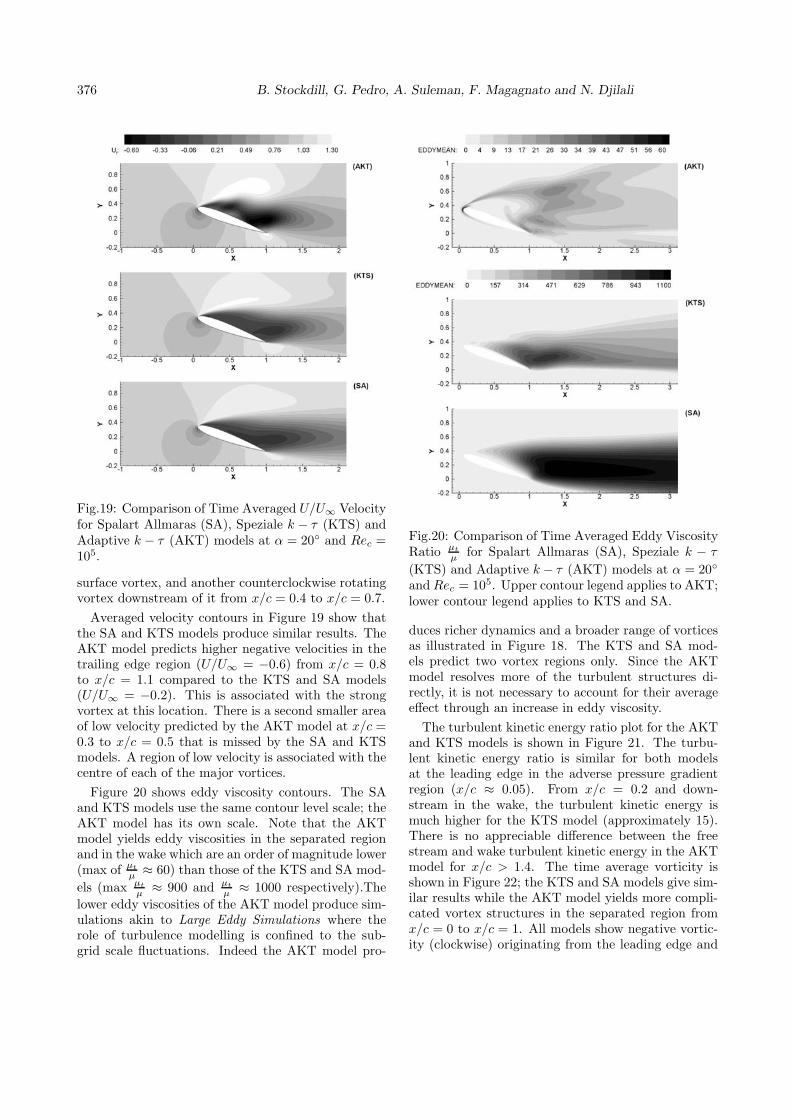
Averaged velocity contours in Figure 19 show thatthe SA and KTS models produce similar results. TheAKT model predicts higher negative velocities in thetrailing edge region (U/U∞ = −0.6) from x/c = 0.8to x/c = 1.1 compared to the KTS and SA models(U/U∞ = −0.2). This is associated with the strongvortex at this location. There is a second smaller areaof low velocity predicted by the AKT model at x/c =0.3 to x/c = 0.5 that is missed by the SA and KTSmodels. A region of low velocity is associated with thecentre of each of the major vortices.

Figure 20 shows eddy viscosity contours. The SAand KTS models use the same contour level scale; theAKT model has its own scale. Note that the AKTmodel yields eddy viscosities in the separated regionand in the wake which are an order of magnitude lower(max of μt

μ ≈ 60) than those of the KTS and SA mod-els (max μt

μ ≈ 900 and μt

μ ≈ 1000 respectively).Thelower eddy viscosities of the AKT model produce sim-ulations akin to Large Eddy Simulations where therole of turbulence modelling is confined to the sub-grid scale fluctuations. Indeed the AKT model pro-

Fig.20: Comparison of Time Averaged Eddy ViscosityRatio μt

μ for Spalart Allmaras (SA), Speziale k − τ

(KTS) and Adaptive k − τ (AKT) models at α = 20◦

and Rec = 105. Upper contour legend applies to AKT;lower contour legend applies to KTS and SA.

duces richer dynamics and a broader range of vorticesas illustrated in Figure 18. The KTS and SA mod-els predict two vortex regions only. Since the AKTmodel resolves more of the turbulent structures di-rectly, it is not necessary to account for their averageeffect through an increase in eddy viscosity.

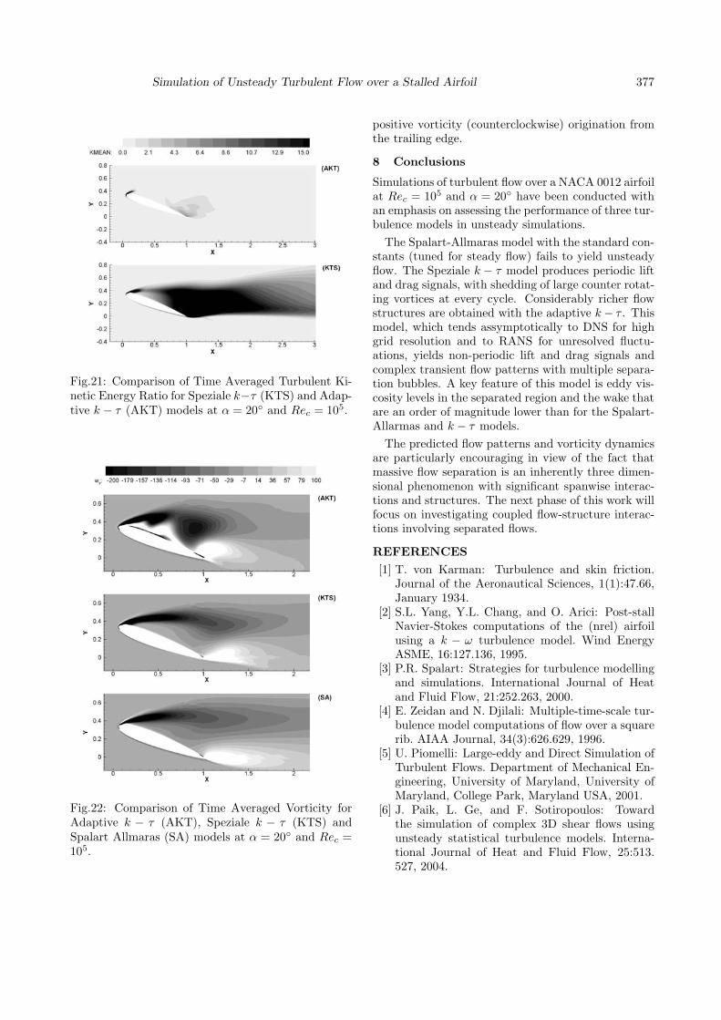
The turbulent kinetic energy ratio plot for the AKTand KTS models is shown in Figure 21. The turbu-lent kinetic energy ratio is similar for both modelsat the leading edge in the adverse pressure gradientregion (x/c ≈ 0.05). From x/c = 0.2 and down-stream in the wake, the turbulent kinetic energy ismuch higher for the KTS model (approximately 15).There is no appreciable difference between the freestream and wake turbulent kinetic energy in the AKTmodel for x/c > 1.4. The time average vorticity isshown in Figure 22; the KTS and SA models give sim-ilar results while the AKT model yields more compli-cated vortex structures in the separated region fromx/c = 0 to x/c = 1. All models show negative vortic-ity (clockwise) originating from the leading edge and

Simulation of Unsteady Turbulent Flow over a Stalled Airfoil 377

Fig.21: Comparison of Time Averaged Turbulent Ki-netic Energy Ratio for Speziale k−τ (KTS) and Adap-tive k − τ (AKT) models at α = 20◦ and Rec = 105.

Fig.22: Comparison of Time Averaged Vorticity forAdaptive k − τ (AKT), Speziale k − τ (KTS) andSpalart Allmaras (SA) models at α = 20◦ and Rec =105.

positive vorticity (counterclockwise) origination fromthe trailing edge.

8 Conclusions

Simulations of turbulent flow over a NACA 0012 airfoilat Rec = 105 and α = 20◦ have been conducted withan emphasis on assessing the performance of three tur-bulence models in unsteady simulations.

The Spalart-Allmaras model with the standard con-stants (tuned for steady flow) fails to yield unsteadyflow. The Speziale k − τ model produces periodic liftand drag signals, with shedding of large counter rotat-ing vortices at every cycle. Considerably richer flowstructures are obtained with the adaptive k − τ . Thismodel, which tends assymptotically to DNS for highgrid resolution and to RANS for unresolved fluctu-ations, yields non-periodic lift and drag signals andcomplex transient flow patterns with multiple separa-tion bubbles. A key feature of this model is eddy vis-cosity levels in the separated region and the wake thatare an order of magnitude lower than for the Spalart-Allarmas and k − τ models.

The predicted flow patterns and vorticity dynamicsare particularly encouraging in view of the fact thatmassive flow separation is an inherently three dimen-sional phenomenon with significant spanwise interac-tions and structures. The next phase of this work willfocus on investigating coupled flow-structure interac-tions involving separated flows.

REFERENCES[1] T. von Karman: Turbulence and skin friction.

Journal of the Aeronautical Sciences, 1(1):47.66,January 1934.

[2] S.L. Yang, Y.L. Chang, and O. Arici: Post-stallNavier-Stokes computations of the (nrel) airfoilusing a k − ω turbulence model. Wind EnergyASME, 16:127.136, 1995.

[3] P.R. Spalart: Strategies for turbulence modellingand simulations. International Journal of Heatand Fluid Flow, 21:252.263, 2000.

[4] E. Zeidan and N. Djilali: Multiple-time-scale tur-bulence model computations of flow over a squarerib. AIAA Journal, 34(3):626.629, 1996.

[5] U. Piomelli: Large-eddy and Direct Simulation ofTurbulent Flows. Department of Mechanical En-gineering, University of Maryland, University ofMaryland, College Park, Maryland USA, 2001.

[6] J. Paik, L. Ge, and F. Sotiropoulos: Towardthe simulation of complex 3D shear flows usingunsteady statistical turbulence models. Interna-tional Journal of Heat and Fluid Flow, 25:513.527, 2004.

378 B. Stockdill, G. Pedro, A. Suleman, F. Magagnato and N. Djilali

[7] F. Magagnato and M. Gabi: A new adaptive tur-bulence model for unsteady flow fields in rotatingmachinery. International Journal of Rotating Ma-chinery, 8(3):175.183, 2002.

[8] J.C. Muti Lin and L.L. Pauley: Low-Reynoldsnumber separation on an airfoil. AIAA Journal,34(8):1570.1577, August 1996.

[9] E. Chaput: Aerospatiale-a airfoil. Contribution inecarp-european computational aerodynamics re-search project: Validation of cfd codes and as-sessment of turbulent model. Notes on Numeri-cal Fluid Mechanics, Vieweg Verlag, 58:327.346,1997.

[10] C. Weber and F. Ducros: Large eddy andReynolds-averaged Navier-Stokes simulations ofturbulent flow over an airfoil. IJCFD, 13:327.355,2000.

[11] L. Davidson: Navier-Stokes stall predictions us-ing an algebraic Reynolds-stress model. Journalof Spacecraft and Rockets, 29(6):794.800, Decem-ber 1992.

[12] C.M. Rhie and W.L. Chow: Numerical studyof the turbulent flow past an airfoil with trail-ing edge separation. AIAA Journal, 21(11):1525.1532, November 1983.

[13] A. Roshko: On the drag and shedding frequencyof two-dimensional bluff bodies. Technical ReportNACA TN 3169, California Institute of Technol-ogy, 1954.

[14] G. Pedro, A. Suleman, and N. Djilali: A numer-ical study of the propulsive efficiency of a flap-ping hydrofoil. International Journal of NumericalMethods in Fluids, 42:493.526, 2003.

[15] N. Gregory and C.L. OfReilly: Low-speed aerody-namic characteristics of NACA0012 aerofoil sec-tion, including the effects of upper surface rough-ness simulating hoar frost. Technical report, Na-tional Physical Laboratory Aerodynamics Divi-sion, 1970.

[16] K.B.M.Q. Zaman, D.J. McKinzie, and C.L. Rum-sey: A natural low-frequency oscillation of theflow over an airfoil near stalling conditions. Jour-nal of Fluid Mechanics, 202:403.442, 1989.

[17] R.D. Blevins: Flow Induced Vibration. Van Nos-trand Reinhold, New York, second edition, 1990.

[18] H. Schlichting: Boundary-Layer Theory.McGraw-Hill, sixth edition, 1968.

[19] P.R. Spalart and S.R. Allmaras: A one-equationturbulence model for aerodynamic flows. AIAAPaper 92-0439, 1992.

[20] N. Djilali, I.S. Gartshore, and M. Salcudean: Tur-bulent flow around a bluff rectangular plate. PartII: Numerical predictions. ASME Journal of Flu-

ids Engineering, 113:60.67, 1991.[21] C.G. Speziale, R. Abid, and E.C. Anderson: Crit-

ical evaluation of two-equation models for near-wall turbulence. AIAA Journal, 30(2):324.331,1992.

[22] S.T. Johansen, J. Wu, and W. Shyy: Filterbased unsteady RANS computations. Interna-tional Journal of Heat and Fluid Flow, 25:10.21,2004.

[23] T.J. Craft, B.E. Launder, and K. Suga: Devel-opment and application of a cubic eddy-viscositymodel of turbulence. International Journal ofHeat and Fluid Flow, 17:108.115, 1995.

[24] T.J. Craft, B.E. Launder, and K. Suga: Pre-diction of turbulent transitional phenomena witha nonlinear eddy-viscosity model. InternationalJournal of Heat and Fluid Flow, 18:15.28, 1997.

[25] F. Magagnato: SPARC Structured PArallelResearch Code. Department of Fluid Machin-ery, University of Karlsruhe (TH), Kaiserstrasse12,D76131 Karlsruhe, Germany, 1998.

[26] R.H. Pletcher and K-H Chen: On solving thecompressible Navier-Stokes equations for un-steady flows at very low Mach numbers. AIAA,1993.

[27] D. Greer and P. Hamroy: Design and predic-tions for a high-altitude (low-Reynolds-number)aerodynamic flight experiment. Technical ReportTM1999-206579, NASA, 1999.

[28] F-B Hsiao, C-F Liu, and Z. Tang: Aerodynamicperformance and flow structure studies of a lowReynolds number airfoil. AIAA Journal, 27(2),February 1989.

[29] R. Horn and P.G. Vicente: Comprehensive anal-ysis of turbulent flows around an NACA0012 pro-file, including dynamics stall effects. InternationalJournal of Computer Applications in Technology,11(3):230.251, 1998.