Short Introduction to the Lambda-calculus - Mbox.dmi.unict.it
46
15/11/2005 11:46 AM Lambda-calculus Pagina 1 di 46 http://www.dmi.unict.it/~barba/LinguaggiII.html/READING_MATERIAL/LAMBDACALCULUS/LAMBDACALCULUS.1.HTM Short Introduction to the Lambda-calculus Franco Barbanera with the collaboration of Claudia & Tiziana Genovese and Massimiliano Salfi
Transcript of Short Introduction to the Lambda-calculus - Mbox.dmi.unict.it
15/11/2005 11:46 AMLambda-calculus
Pagina 1 di 46http://www.dmi.unict.it/~barba/LinguaggiII.html/READING_MATERIAL/LAMBDACALCULUS/LAMBDACALCULUS.1.HTM
ShortIntroduction
to the Lambda-calculus
Franco Barbanera
with the collaboration of Claudia & Tiziana Genovese
and Massimiliano Salfi
15/11/2005 11:46 AMLambda-calculus
Pagina 2 di 46http://www.dmi.unict.it/~barba/LinguaggiII.html/READING_MATERIAL/LAMBDACALCULUS/LAMBDACALCULUS.1.HTM
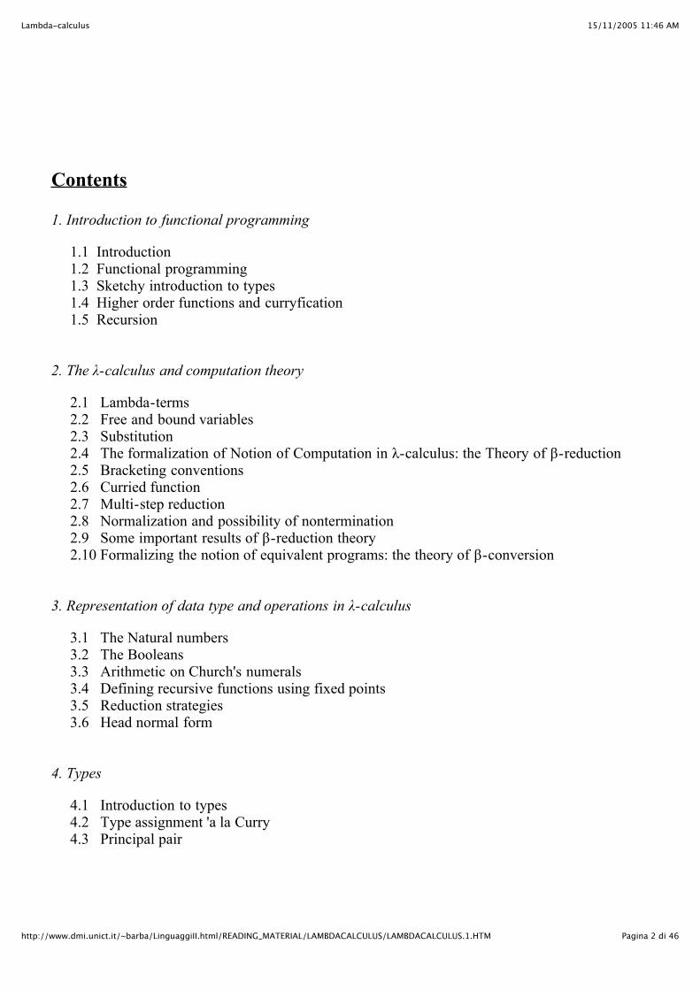
Contents
1. Introduction to functional programming
1.1 Introduction 1.2 Functional programming 1.3 Sketchy introduction to types 1.4 Higher order functions and curryfication 1.5 Recursion
2. The λ-calculus and computation theory
2.1 Lambda-terms 2.2 Free and bound variables 2.3 Substitution 2.4 The formalization of Notion of Computation in λ-calculus: the Theory of β-reduction 2.5 Bracketing conventions 2.6 Curried function 2.7 Multi-step reduction 2.8 Normalization and possibility of nontermination 2.9 Some important results of β-reduction theory 2.10 Formalizing the notion of equivalent programs: the theory of β-conversion
3. Representation of data type and operations in λ-calculus
3.1 The Natural numbers 3.2 The Booleans 3.3 Arithmetic on Church's numerals 3.4 Defining recursive functions using fixed points 3.5 Reduction strategies 3.6 Head normal form
4. Types
4.1 Introduction to types 4.2 Type assignment 'a la Curry 4.3 Principal pair
15/11/2005 11:46 AMLambda-calculus
Pagina 3 di 46http://www.dmi.unict.it/~barba/LinguaggiII.html/READING_MATERIAL/LAMBDACALCULUS/LAMBDACALCULUS.1.HTM
1. Introduction to functional programming
1.1 Introduction
What does computing mean? Roughly, to transform information from an implicit into an explicit form.
But this notion means nothing unless we make it precise, formal, by defining a computationalmodel. What is a Computational model? A particular formalization of the notions connected to the concept of "computing". The rather vague concept of computing can be formalized in several different ways, that is bymeans of several different computational models: the Lambda-calculus, the Turing machine, etc. "To program" means to specify a particular computation process, in a language based on aparticular computational model.
Functional programming languages are based on the Lambda-calculus computational model. Imperative programming languages are based on the Turing-machine computational model.
The fundamental concepts in imperative programming languages (coming from the TuringMachine model) are:
storevariable - something it is possible to modify ("memory cell")assignmentiteration
In functional programming these concepts are absent (or, in case they are present, have adifferent meaning). Instead, in it we find:
expressionrecursion - different from the notion of iterationevaluation - different from the notion of execution:
when we evaluate a mathematical expression we do not modify anything.variable - intended in a mathematical sense:
unknown entityabstraction from a concrete value
15/11/2005 11:46 AMLambda-calculus
Pagina 4 di 46http://www.dmi.unict.it/~barba/LinguaggiII.html/READING_MATERIAL/LAMBDACALCULUS/LAMBDACALCULUS.1.HTM
1.2 Functional programming
A program in a functional language is a set of function definitions and an expression usuallyformed using the defined functions. The Interpreter of the language evaluates this expression bymeans of a discrete number of computation steps, in such a way its meaning turns out to berepresented in an explicit way. In general in programming we have not to produce anything; infunctional programming, in particular, what we modify is only the representation of theinformation.
A function can be defined in several ways.
Example:
f: R -> R , g: R -> R f '' - 6g' = 6 sen x 6g'' + a2 f ' = 6 cos x f(0) = 0, f '(0) = 0, g(0) = 1, g'(0) = 1
This set of equations precisely identify two precise f and g.
A function definition in a functional programming language, however, has not simply to uniquelyidentify a mathematical function on a domain of objects, but it is also necessary that such adefinition provides a means to compute the function on a given argument.
Example: function definition in Scheme and in Haskell
(define Inctwo (lambda (n) (+ n 2)))
Inctwo n = n + 2
To evaluate an expression in Scheme (as in Haskell) means to look for a sub-expression whichis the application of a function to some arguments and then to evaluate the body of the functionin which the formal parameter is replaced by the actual parameter. In this way, in a sense, wemake the meaning of such sub-expression more explicit.
Example: let us evaluate Inctwo 3
Inctwo 3 Inctwo is a user defined function, and it is applied to an argument, so we take thebody of the function, replace the formal parameter n by the actual parameter 3, obtaining 3+2, and then we evaluate 3+2 obtaining 5
In the example above we have seen two kinds of computational steps from Inc 3 to 5. In the firstone we have simply substituted in the body of the function the formal parameter by the actualparameter, the argument, and in the second one we have computed a predefined function. Weshall see that the essence of the notion of computation in functional programming is indeedembodied by the first type of computational step. The simple operation of replacing thearguments of a function for its formal parameters in its body contains all the computing power offunctional programming. Any sort of computation in functional programming could indeed be
15/11/2005 11:46 AMLambda-calculus
Pagina 5 di 46http://www.dmi.unict.it/~barba/LinguaggiII.html/READING_MATERIAL/LAMBDACALCULUS/LAMBDACALCULUS.1.HTM
functional programming. Any sort of computation in functional programming could indeed bedefined in terms of this one. We shall see this later, when we shall represent this sort ofcomputational step with the beta-reduction rule in the lambda calculus and we shall see that, ifone wish, any possible computation can be defined in terms of this beta-rule.
When we evaluate an expression there are sometimes more than one sub-expression one canchoose and hence different possible evaluation paths can be followed. An evaluation strategy isa policy enabling to decide on which sub-expression we shall perform the next evaluation step.Some evaluation strategies could led me in a never ending path (this fact is unavoidable); but Iwould like to be sure that all finite path lead me to the very same value (this will be guaranteedby the Church-Rosser Theorem of the Lambda-calculus).
Example: In Haskell
inf = inf // definition of the value inf alwayseven x = 7 // definition of the function alwayseven alwayseven inf // expression to be evaluated
Two possible choices in the evaluation of alwayseven Inf:
. 1 We evaluate inf first (the evaluation strategy of Scheme).
. 2 We evaluate alwayseven inf first (the evaluation strategy of Haskell, a lazy language).case 1. Replace inf by inf => we go on endlessly case 2. Replace alwayseven inf by 7 => we terminate in a single step.
One of the distinguishing features in a programming language is the evaluation strategy it uses.
We know how to define the function factorial in a recursive way. Let us give now an example ofmutually recursive functions.
even x=if x=0 then true else odd(x-1) odd x=if x=0 then false else even(x-1)
With our recursive definitions we do not only specify functions, but we also provide a method tocompute then: a recursive definition definition says that the left-hand side part of the equation isequivalent (has the same "meaning") of the right-hand side. The right-hand side, however, has itsmeaning expressed in a more explicit way. We can replace the left-hand side part with the right-hand one in any expression without modifying its meaning. We can notice that in order to evaluate "even 3" we can follow different evaluation strategies. Itis also possible to perform more reductions in parallel, that is to replace two or more sub-expressions with equivalent sub-expression (reduction step) at the same time. A similar thing isnot possible in imperative languages since we need to take into account the problem of sideeffects: running in parallel the instructions of the subprograms computing two functions F1 and F2 canproduce strange results, since the two subprograms could use (and modify) the value of globalvariables which can affect the results produced by the two functions. Of course, because of thepresence of global variables, the value of a function can depend on time and on how many timeswe have computed it before. (in general in imperative languages it is difficult to be sure that weare programming actual mathematical functions). We have not the above mentioned problems infunctional programming languages, since there not exists side effects (there are no global
15/11/2005 11:46 AMLambda-calculus
Pagina 6 di 46http://www.dmi.unict.it/~barba/LinguaggiII.html/READING_MATERIAL/LAMBDACALCULUS/LAMBDACALCULUS.1.HTM
functional programming languages, since there not exists side effects (there are no globalmodifyable variables). What we define are therefore actual mathematical functions; hence in anexpression the value of any sub-expression does not depend on the way we evaluate it or otherones, that is the same expression always denotes the same value (a property called referentialtransparency).
1.3 Sketchy introduction to types
Some functional programing languages are typed. A type, in general, can be looked at as apartial specification of a program. These partial specifications, according to the particular typesytem of the language considered, can be more or less detailed.
By means of types we can avoid errors like:
true + 3
in fact the interpreter knows that
+:: int x int → int
In (strongly) typed languages this error is detected by the interpreter, hence before the program isrun. In not (strongly) typed languages this error is detected at run-time (the program stops duringits run). In some typed functional languages it is possible to define polymorphic functions, that iswhich, roughly, have the same behaviour on arguments of different types (these functions have apolymorphic type: a type describing a whole set of (uniform) behaviours).
Example:
ident:: a → a (where a is a type-variable, it denotes a "generic" type.) ident x = x
We shall study very simple types, like int->bool (it simply specifies that a function (program)with this type has an integer as an argument and a boolean as result). Notice, however, that thereexist type systems so expressive that they can specify in a very precise way what a functioncomputes. For istance
Forall x : Int Exists y: Int . y=x+1
saying that a function with this type have integers as argument, integers as results, and that itcomputes the successor function (of course it does not specify how the successor of a giveninteger is computed).
1.4 Higher order functions and curryfication
15/11/2005 11:46 AMLambda-calculus
Pagina 7 di 46http://www.dmi.unict.it/~barba/LinguaggiII.html/READING_MATERIAL/LAMBDACALCULUS/LAMBDACALCULUS.1.HTM
In functional programming languages functions are treated as any other object. Hence they can begiven as argument to other functions or be the result of a function. Function that can havefunctions as argument or result are called higher-order functions. This enables us to introduce thenotion of curryfication, a relevant concept in functional languages. To currify means to transforma function f of arity n, in an higher-order function fcur of arity 1 such that also fcur(a1) is a higherorder function of arity 1, and so are fcur(a1)(a2) up to fcur(a1)(a2)..(an-1) and such thatf(a1,..,an)=fcur(a1)..(an). A binary function of type:
A x B → C
is currifyed to a function of type:
A → (B → C)
where any function arity is 1. (Higher-order functions and curryfication are treated in Section1.7 of the reference below.)
Note: Also in imperative languages it is possible to program functions which have functions as arguments, but in general what isgiven as argument is simply a pointer to some code (which needs to be treated as such).
1.5 Recursion
The computational power of functional languages is provided by the recursion mechanism; henceit is natural that in functional languages it is much easier to work on recursively defineddatatypes.
Example:
the datatype List is recursively defined as follows: an element of List is either [] or elem : list.
BinaryTree (unlabelled) is another example: an element of BinaryTree is either EmptyTree or a root at the top of two elements ofBinaryTree.
Notice that there is a strong relation between the Induction principle as a mathematical proof tooland Recursion a computation tool.
One starts from the basis case;By assuming a property to hold for n, one shows the property for n+1
(this is the principle of numerical induction; it corresponds to the mechanism of defining afunction on numbers by recursion; We shall see that induction principles on complex inductivedata types correspond to the general mechanism of defining function by recursion)
Disadvantages of functional programming We are used to work on data structures that are intrinsically tied to the notion of "modification",
15/11/2005 11:46 AMLambda-calculus
Pagina 8 di 46http://www.dmi.unict.it/~barba/LinguaggiII.html/READING_MATERIAL/LAMBDACALCULUS/LAMBDACALCULUS.1.HTM
We are used to work on data structures that are intrinsically tied to the notion of "modification",so we usually thing that an element of a data type can be modified. We need to be careful, infunctional programming a function that, say, take a numerically labeled tree and increment itslabels, does not modify the input. It simply builds a new tree with the needed characteristics. Thesame when we push or pop elements from a stack: each time a new stack is created. This cause agreat waste of memory (the reason why in implementations of functional programming languagesa relevant role is played by the Garbage Collector). Of course there can be optimizations andtricks used in implementation that can limit this phenomenon.
Text to use: R. Plasmeijer, M. van Eekelen, "Functional Programming and Parallel Graph Rewriting", Addison-Wesley, 1993.Cap. 1 (basic concepts)
2. The λ-calculus and computation theory
2.1 Lambda-terms
The fundamental concepts the Lambda-calculus is based on are:
variable ( formalisable by x, y ,z,…)abstraction (formalisable by λx.M where M is a term and x a variable)application (formalizable by M N, where M and N are terms )
We have seen that these are indeed fundamental notions in functional programming. It seems thatthere are other important notions: basic elements, basic operators and the possibility of givingnames to expressions, but we shall see that the three above notions, are the real fundamental onesand we can found our computational model just on these concepts. Out of the formalization ofthese three concepts we form the lambda-terms. These terms will represent both programs anddata in our computational model (whose strenght is indeed also the fact it does not distinguishbetween "programs" and "data".)
The formal definition of the terms of the Lambda-calculus (lambda-terms) is given by thefollowing grammar:
Λ ::= X | (ΛΛ) | λX.Λ
where Λ stands for the set of lambda-terms and X is a metavariable that ranges over the(numerable) set of variables (x, y, v, w, z, x2, x2,...) Variable and application are well-known concepts, but what is abstraction ? In our sense it is a notion tied to that of "abstracting from a concrete value" (disregarding thespecific aspects of a particular object, that in our case is an input.) It is needed to formalize thenotion of anonymous functions creation (when we have given the example of definition inHaskell of the function fact, we have done indeed two things: we have specified a function andwe have given to it a name, fact. To be able to specify a function is essential in ourcomputational model, but we can avoid to introduce in our model the notion of "giving a name toa function". But how is it possible to define a function like fact without being able to refer to ittrought its name??? We shall see)
Example of (functional) abstraction:
15/11/2005 11:46 AMLambda-calculus
Pagina 9 di 46http://www.dmi.unict.it/~barba/LinguaggiII.html/READING_MATERIAL/LAMBDACALCULUS/LAMBDACALCULUS.1.HTM
We can specify the square function by saying that it associates 1 to 1*1, 2 to 2*2, 3 to 3*3,ecc. In the specification of the function the actual values of the possible particular inputs arenot needed, that is we can abstract from the actual values of the input by simply saying thatthe function square associates the generic input x to x*x. We can use the mathematical notation x |— x*x to specify a particular relation betweendomain and codomain; this is a mathematical notation to specify a function without assigningto it a particular name (an anonymous function).
In Lambda-calculus we describe the relation input-output by means of the lambda-abstractionoperator: λx. x*x (anonymous function associating x to x*x). Other notions, usually consideredas primitive, like basic operators (+, *, -, ...) or natural numbers are not necessary in thedefinition of the terms of our functional computational model (indeed we shall see that they canbe considered, in our model, as derived concepts.)
2.2 Free and bound variables
Definition of free variable (by induction on the structure of the term) We define the FV (Free Variables), the function which gives the free variables of a term as:
FV(x) = x FV(PQ) = FV(P) U FV(Q) FV(λx.P) = FV(P) \ x
Definition of bound variable (by induction on the structure of the term) The function BV (Bound Variables) is defined by:
BV(x) = Φ (the emptyset)BV(PQ) = BV(P) U BV(Q) BV(λx.P) = x U BV(P)
In a term M we abstract with respect to the variable x (λx.M) then x is said to be bound in M.
2.3 Substitution
With the notation M [L / x] we denote the term M in which any free variable x in M is replacedby the term L.
Definition of substitution (by induction on the structure of the term) 1. If M is a variable (M = y) then:
y [L/x] ≡L if x=y
y if x≠y
15/11/2005 11:46 AMLambda-calculus
Pagina 10 di 46http://www.dmi.unict.it/~barba/LinguaggiII.html/READING_MATERIAL/LAMBDACALCULUS/LAMBDACALCULUS.1.HTM
2. If M is an application (M = PQ) then:
PQ [L/x] = P[L/x] Q[L/x]
3. If M is a lambda-abstraction (M = λy.P) then:
λy.P [L/x] ≡λy.P if x=y
λy.(P [L /x]) if x≠y
Notice that in a lambda abstraction a substitution is performed only in case the variable tosubstitute is not bound.
This definition, however, is not completely correct. Indeed it does not prevent some harmfulambiguities and errors:
Example:
(λx.z) and (λy.z) they both represent the constant function which returns z for anyargument
Let us assume we wish to apply to both these terms the substitution [x / z] (we replace x forthe free variable z). If we do not take into account the fact that the variable x is free in theterm x and bound in (λx.z) we get:
(λx.z) [x / z] => λx.(z[x / z]) => λx.x representing the identity function (λy.z) [x / z] => λy.(z[x/ z]) => λy.x representing the function that returns always x
This is absurd, since both the initial terms are intended to denote the very same thing (aconstant function returning z), but by applying the substitution we obtain two terms denotingvery different things.
Hence a necessary condition in order the substitution M[L/x] be correctly performed isFV(L) and BV(M) be disjunct sets.
Example:
let us consider the following substitution:
(λz.x) [zw/x]
The free variable z in the term to be substituted would become bound after the substitution.This is meaningless. So, what it has to be done is to rename the bound variables in the termon which the substitution is performed, in order the condition stated above be satisfied:
(λq.x) [zw/x]; now, by performing the substitution, we correctly get: (λq.zw)
15/11/2005 11:46 AMLambda-calculus
Pagina 11 di 46http://www.dmi.unict.it/~barba/LinguaggiII.html/READING_MATERIAL/LAMBDACALCULUS/LAMBDACALCULUS.1.HTM
2.4 The formalization of the notion of computation in λ-calculus: TheTheory of β-reduction
In a functional language to compute means to evaluate expressions, making the meaning of theexpression itself more and more explicit. In our computational model for functionalprogramming, the Lambda-calculus, we then need to formalize also what a computation is. Inparticular we need to formalize the notion of "basic computational step".
Formalization of the notion of computational step (the notion of β-reduction):
(λx.M) N →β M [N/x]
This notion of reduction expresses what we intend by "computational step": Inside the body M ofthe function λx.M the formal parameter x is replaced by the actual parameter (argument) given tothe function.
Note: A term like (λx.M)N is called redex, while M[N/x] is its contractum.
What does it mean that a computation step is performed on a term? It means that the term contains a subterm which is a redex and such a redex is substituted by itscontractum (β-reduction is applied on that redex.)More formally, a term M β-reduces in one-step to a term N if N can be obtained out of M byreplacing a subterm of M of the form (λx.P)Q by P[Q/x]
Example:
(λx. x*x) 2 => 2*2 => 4
here the first step is a β-reduction; the following computation is the evaluation of themultiplication function. We shall see how this last computation can indeed be realized bymeans of a sequence of basic computational steps (and how also the number 2 and thefunction multiplication can be represented by λ-terms).
Example:
(λz. (zy) z) (x (xt)) →β (x (xt) y) (x (xt))
Example:
(λy. zy) (xy) →β z(xy) here it could be misleading the fact that the variable y appears once free and once bound. Asa matter of fact these two occurrences of y represent two very different things (in fact thebound occurrence of y can be renamed without changing the meaning of the term, the freeone not). Notice that even if there is this small ambiguity, the beta reduction can be
15/11/2005 11:46 AMLambda-calculus
Pagina 12 di 46http://www.dmi.unict.it/~barba/LinguaggiII.html/READING_MATERIAL/LAMBDACALCULUS/LAMBDACALCULUS.1.HTM
one not). Notice that even if there is this small ambiguity, the beta reduction can beperformed without changing the name of the bound variables. Why?
The notion of alpha-convertibilityA bound variable is used to represent where, in the body of a function, the argument of thefunction is used. In order to have a meaningful calculus, terms which differ just for the names oftheir bound variables have to be considered identical. We could introduce the notion of differingjust for bound variables names in a very formal way, by defining the relation of α-convertibility.Here is an example of two terms in such a relation.
λz.z =α λx.x
We do not formally define here such a relation. For us it is sufficient to know that two terms are α-convertible whenever one can be obtained from the other by simply renaming the boundvariables. Obviously alpha convertibility mantains completely unaltered both the meaning of the term andhow much this meaning is explicit. From now on, we shall implicitely work on λ-terms moduloalpha conversion. This means that from now on two alpha convertible terms like λz.z and λx.x arefor us the very same term.
Example:
(λz. ((λt. tz) z)) z
All the variables, except the rightmost z, are bound, hence we can rename them (apply α-conversion). The rightmost z, instead, is free. We cannot rename it without modifying themeaning of the whole term.
It is clear from the definition that the set of free variables of a term is invariant by α-conversion,the one of bound variables obviously not.
A formal system for beta-reductionIf one wishes to be very precise, it is possible to define a formal system expressing in a detailedway the notion of one-step evaluation of a term, that is of one-step beta reduction. First recall roughly what a formal system is.
Definition A formal system is composed by axioms and inference rules enabling us to deduce "Judgements"
Example:
In logics we have formal systems enabling to infer the truth of some propositions, that is thejudgments we derive are of the form "P is true".
We can now introduce a formal system whose only axiom is the β-rule we have seen before:
15/11/2005 11:46 AMLambda-calculus
Pagina 13 di 46http://www.dmi.unict.it/~barba/LinguaggiII.html/READING_MATERIAL/LAMBDACALCULUS/LAMBDACALCULUS.1.HTM
———————————(λx. M) N →β M [N/x]
and whose inference rules are the following:
if
then we can infer
P →β P'—————————λx. P →β λx. P'
P →β P'—————————
L P →β L P'
P →β P'—————————
P L →β P' L
The judgements we derive in the formal system defined above have the form M →β M' and areinterpreded as "the term M reduces to the term M' in one step of computation (β-reduction)".
Example:
in this formal system we can have the following derivation:
(λx.x) y → y —————————— (zz) ((λx.x) y) → (zz) y
——————————————— λw.((zz) ((λx.x) y)) → λw ((zz) y)
This is a (very formal) way to show that the term λw.((zz) ((λx.x) y)) reduces in one step to theterm λw.((zz) y) (less formally, and more quickly, we could have simply spotted the redex(λx.x) y inside the term and replaced it by its contractum y)
Actually we are defining a binary relation on lambda-terms, beta reduction, and we have seenthat this can be done informally by saying that a term M is in the relation →β with a term N ( Mβ-reduces with one step to N) if N can be obtained by replacing a subterm of M of the form(λx.P)Q by P[Q/x]
2.5 Bracketing conventions
Abbreviating nested abstractions and applications will make curried function easier to write. Weshall abbreviate
(λx1.(λx2. ... . (λxn.M) ... ) by (λx1x2 ... xn.M)
( ... ((M1M2)M3) ... Mn) by (M1M2M3 ... Mn)
We also use the convention of dropping outermost parentheses and those enclosing the body ofan abstraction.
Example:
15/11/2005 11:46 AMLambda-calculus
Pagina 14 di 46http://www.dmi.unict.it/~barba/LinguaggiII.html/READING_MATERIAL/LAMBDACALCULUS/LAMBDACALCULUS.1.HTM
(λx.(x (λy.(yx)))) can be written as λx.x(λy.yx)
2.6 Curried functions
Let us see what's the use of the notion of curryfication in the lambda-calculus.
As we mentioned before, if we have, say, the addition function, is is always possible to use itscurrified version AddCurr : N → (N → N) and any time we need to use it, say Add(3,5), wecan use instead ((AddCurr(3)) 5). This means that it is not strictly needed to be able to definefunctions of more than one argument, but it is enough to be able to define one argumentfunctions. That is why the λ-calculus, that contains only the strictly essential notions offunctional programming, has only one-argument abstraction.
Notice that not only the use of curried functions does not make us lose computational power, butinstead, can give us more expressive power, since, for instance, if we wish to use a function thatincrements an argument by 3, instead of defining it we can simply use AddCurr(3).
Not all the functional languages have a built-in curryfication feature. Scheme has it not. InScheme any function you define has a fixed arity, 1 or more. If you wish to use a curryfiedversion of a function you have to define it explicitely. In Haskell instead, all function areimplicitly intended to be currified: when you define Add x y = x + y you are indeed definingAddCurr.
2.7 Multi-step reduction
Strictly speaking, M → N means that M reduces to N by exactly one reduction step. Frequently,we are interested in whether M can be reduced to N by any number of steps.
we write M —» N if M → M1 → M2 → ... → Mk ≡ N (K ≥ 0)
It means that M reduces to N in zero or more reduction steps.
Example:
((λz.(zy))(λx.x)) —» y
2.8 Normalization and possibility of non termination
Definition If a term contains no β-redex it is said to be in normal form. For example, λxy.y and xyz are innormal form.
15/11/2005 11:46 AMLambda-calculus
Pagina 15 di 46http://www.dmi.unict.it/~barba/LinguaggiII.html/READING_MATERIAL/LAMBDACALCULUS/LAMBDACALCULUS.1.HTM
normal form.
A term is said to have a normal form if it can be reduced to a term in normal form.
For example:
(λx.x)y
is not in normal form, but it has the normal form y.
Definition: A term M is normalizable (has a normal form, is weakly normalizable) if there exists a term Qin normal form such that
M —» Q
A term M is strongly normalizable, if there exists no infinite reduction path out of M, that is anypossible sequence of β-reductions eventually leads to a normal form.
Example:
(λx.y)((λz.z)t)
is a term not in normal form, normalizable and strongly normalizable too. In fact, the twopossible reduction sequences are:
1. (λx.y)((λz.z) t) → y
2. (λx.y)((λz.z) t) → (λx.y) t) → y
To normalize a term means to apply reductions until a normal form (if any) is reached. Many λ-terms cannot be reduced to normal form. A term that has not normal form is:
(λx.xx)(λx.xx)
This term is usually called Ω.
Although different reduction sequences cannot yield different normal forms, they can yieldcompletely differend outcomes: one could terminate while the other could run forever. Typically,if M has a normal form and admits an infinite reduction sequence, it contains a subterm L havingno normal form, and L can be erased by some reductions. The reduction
(λy.a)Ω → a
reaches a normal form, by erasing the Ω. This corresponds to a call-by-name treatment ofarguments: the argument is not reduced, but substituted 'as it is' into the body of the abstraction. Attempting to normalize the argument generate a non terminating reduction sequence:
15/11/2005 11:46 AMLambda-calculus
Pagina 16 di 46http://www.dmi.unict.it/~barba/LinguaggiII.html/READING_MATERIAL/LAMBDACALCULUS/LAMBDACALCULUS.1.HTM
(λy.a)Ω →(λy.a)Ω → ...
Evaluating the argument before substituting it into the body correspons to a call-by-valuetreatment of function application. In this examples, a call-by-value strategy never reaches thenormal form.
One is naturally led to think that the notion of normal form can be looked at as the abstractformalization in the lambda-calculus of the notion of value in programming languages. In factfor us, intuitively, a value is something that cannot be further evaluated. But we cannot state a-priori what is, in general, a value, since there can be different possible interpretations of thenotion of value. In Scheme, for instance, a lambda expression is a value, that is it cannot beevaluated anymore. Why does the interpreter of Scheme choose to consider a lambda abstraction as a valueindependently from what there is in its body? Well, otherwise it would not be possible to definein Scheme, say, a function that takes an argument and then never stops. So we cannot formalize in general the notion of value, but what is a value has to be specifiedaccording to the context we are in. When we define a functional programming language we needto specify, among other things, also what we intend by value in our language.
2.9 Some important results of β-reduction theory
The normal order reduction strategy consists in reducing, at each step, the leftmost outermost β-redex. Leftmost means, for istance, to reduce L (if it is reducible) before N in a term LN.Outermost means, for instance, to reduce (λx.M) N before reducing M or N (if reducible).Normal order reduction is a call-by-name evaluation strategy.
Theorem (Standardization) If a term has normal form, it is always reached by applying the normal order reduction strategy.
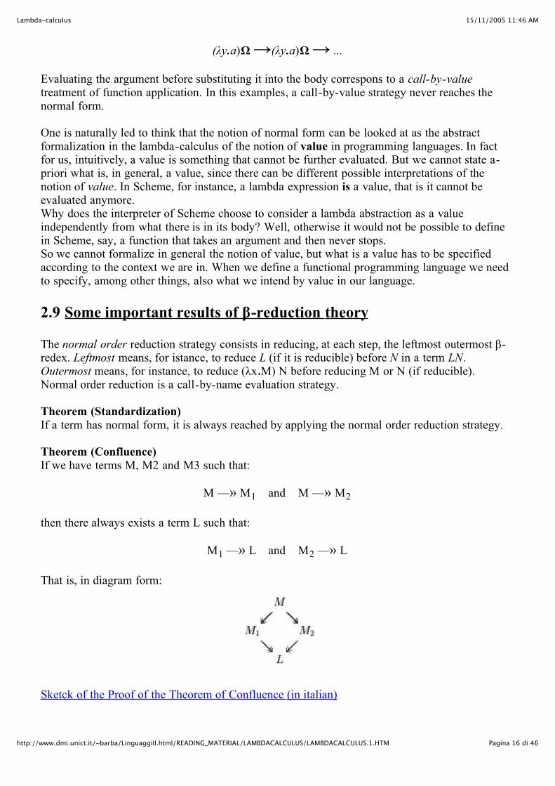
Theorem (Confluence) If we have terms M, M2 and M3 such that:
M —» M1 and M —» M2
then there always exists a term L such that:
M1 —» L and M2 —» L
That is, in diagram form:
Sketck of the Proof of the Theorem of Confluence (in italian)
15/11/2005 11:46 AMLambda-calculus
Pagina 17 di 46http://www.dmi.unict.it/~barba/LinguaggiII.html/READING_MATERIAL/LAMBDACALCULUS/LAMBDACALCULUS.1.HTM
Corollary (Uniqueness of normal form) If a term has a normal form, it is unique.
Proof:Let us suppose to have a generic term M, and let us suppose it has two normal forms N andN'. It means:
M —» N and M —» N'Let us apply, now, the Confluence theorem. Then there exists a term Q such that:
N —» Q and N' —» QBut N and N' are in normal form, then they have not any redex. It means:
N —» Q in 0 steps
then N ≡ Q. Analogously you can prove N' ≡ Q, then N ≡ N'.
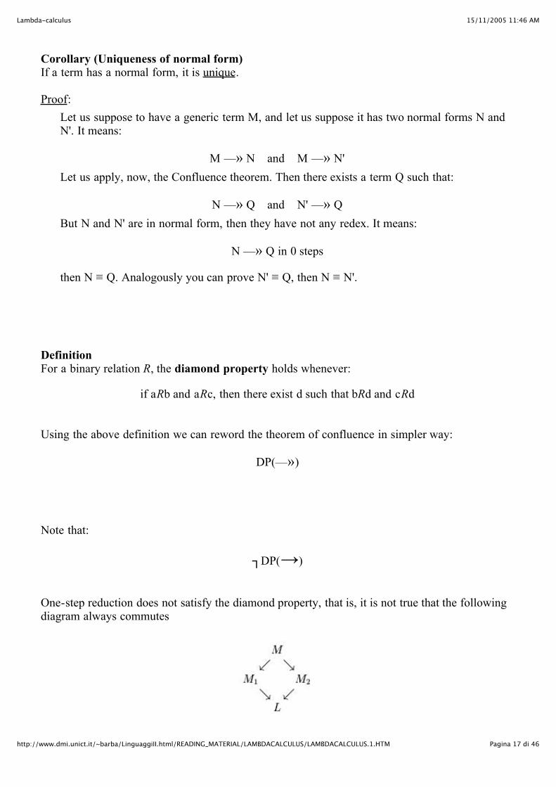
Definition For a binary relation R, the diamond property holds whenever:
if aRb and aRc, then there exist d such that bRd and cRd
Using the above definition we can reword the theorem of confluence in simpler way:
DP(—»)
Note that:
DP(→)
One-step reduction does not satisfy the diamond property, that is, it is not true that the followingdiagram always commutes
15/11/2005 11:46 AMLambda-calculus
Pagina 18 di 46http://www.dmi.unict.it/~barba/LinguaggiII.html/READING_MATERIAL/LAMBDACALCULUS/LAMBDACALCULUS.1.HTM
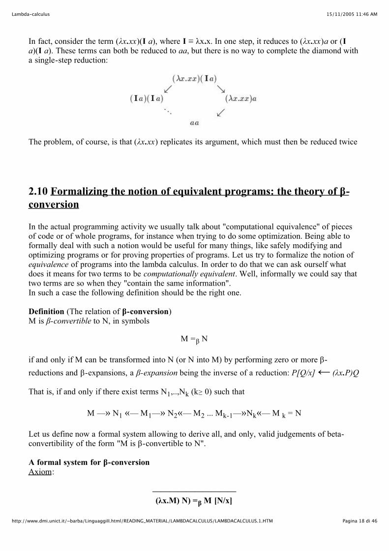
In fact, consider the term (λx.xx)(I a), where I ≡ λx.x. In one step, it reduces to (λx.xx)a or (Ia)(I a). These terms can both be reduced to aa, but there is no way to complete the diamond witha single-step reduction:
The problem, of course, is that (λx.xx) replicates its argument, which must then be reduced twice
2.10 Formalizing the notion of equivalent programs: the theory of β-conversion
In the actual programming activity we usually talk about "computational equivalence" of piecesof code or of whole programs, for instance when trying to do some optimization. Being able toformally deal with such a notion would be useful for many things, like safely modifying andoptimizing programs or for proving properties of programs. Let us try to formalize the notion ofequivalence of programs into the lambda calculus. In order to do that we can ask ourself whatdoes it means for two terms to be computationally equivalent. Well, informally we could say thattwo terms are so when they "contain the same information". In such a case the following definition should be the right one.
Definition (The relation of β-conversion) M is β-convertible to N, in symbols
M =β N
if and only if M can be transformed into N (or N into M) by performing zero or more β-reductions and β-expansions, a β-expansion being the inverse of a reduction: P[Q/x] ← (λx.P)Q
That is, if and only if there exist terms N1,..,Nk (k≥ 0) such that
M —» N1 «— M1—» N2«— M2 ... Mk-1—»Nk«— M k = N
Let us define now a formal system allowing to derive all, and only, valid judgements of beta-convertibility of the form "M is β-convertible to N".
A formal system for β-conversion Axiom:
——————————(λx.M) N) =β M [N/x]
15/11/2005 11:46 AMLambda-calculus
Pagina 19 di 46http://www.dmi.unict.it/~barba/LinguaggiII.html/READING_MATERIAL/LAMBDACALCULUS/LAMBDACALCULUS.1.HTM
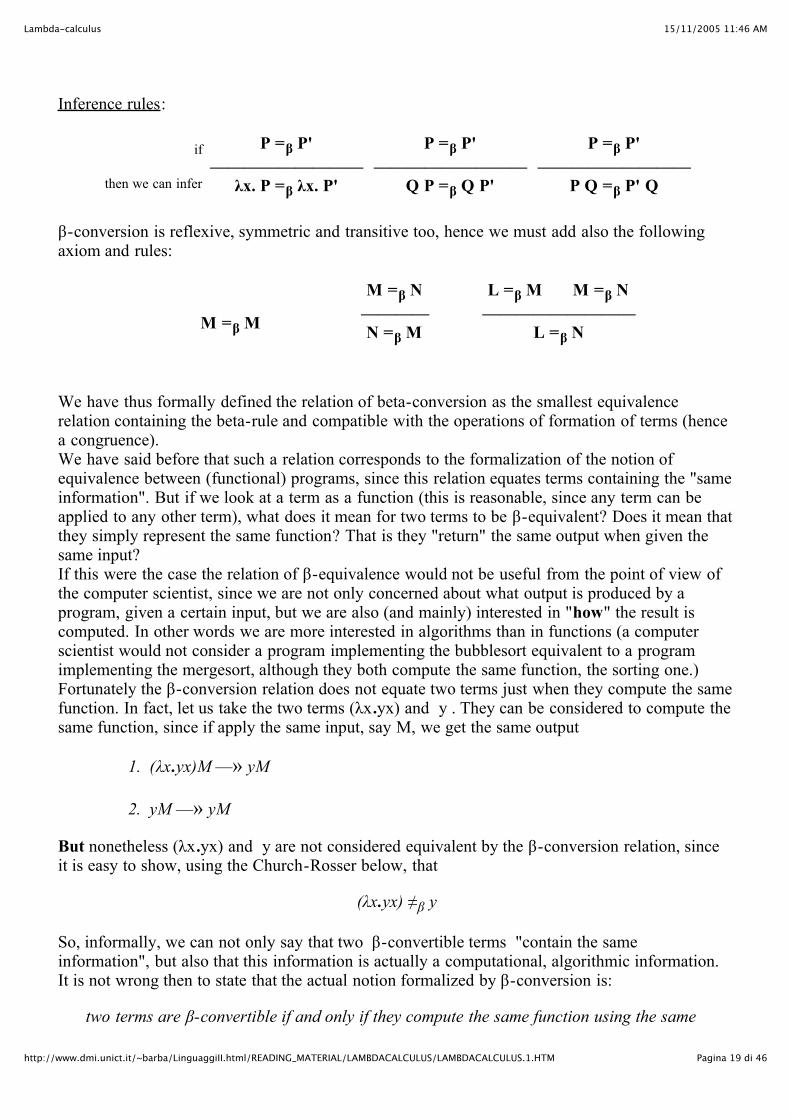
Inference rules:
if
then we can infer
P =β P'—————————λx. P =β λx. P'
P =β P'—————————
Q P =β Q P'
P =β P'—————————
P Q =β P' Q
β-conversion is reflexive, symmetric and transitive too, hence we must add also the followingaxiom and rules:
M =β M
M =β N————N =β M
L =β M M =β N—————————
L =β N
We have thus formally defined the relation of beta-conversion as the smallest equivalencerelation containing the beta-rule and compatible with the operations of formation of terms (hencea congruence).We have said before that such a relation corresponds to the formalization of the notion ofequivalence between (functional) programs, since this relation equates terms containing the "sameinformation". But if we look at a term as a function (this is reasonable, since any term can beapplied to any other term), what does it mean for two terms to be β-equivalent? Does it mean thatthey simply represent the same function? That is they "return" the same output when given thesame input?If this were the case the relation of β-equivalence would not be useful from the point of view ofthe computer scientist, since we are not only concerned about what output is produced by aprogram, given a certain input, but we are also (and mainly) interested in "how" the result iscomputed. In other words we are more interested in algorithms than in functions (a computerscientist would not consider a program implementing the bubblesort equivalent to a programimplementing the mergesort, although they both compute the same function, the sorting one.)Fortunately the β-conversion relation does not equate two terms just when they compute the samefunction. In fact, let us take the two terms (λx.yx) and y . They can be considered to compute thesame function, since if apply the same input, say M, we get the same output
1. (λx.yx)M —» yM
2. yM —» yM
But nonetheless (λx.yx) and y are not considered equivalent by the β-conversion relation, sinceit is easy to show, using the Church-Rosser below, that
(λx.yx) ≠β y
So, informally, we can not only say that two β-convertible terms "contain the sameinformation", but also that this information is actually a computational, algorithmic information.It is not wrong then to state that the actual notion formalized by β-conversion is:
two terms are β-convertible if and only if they compute the same function using the samealgorithm.
15/11/2005 11:46 AMLambda-calculus
Pagina 20 di 46http://www.dmi.unict.it/~barba/LinguaggiII.html/READING_MATERIAL/LAMBDACALCULUS/LAMBDACALCULUS.1.HTM
algorithm.
For a more convincing example, when later on we shall represent numerical mathematicalfunction in the lambda-calculus, you will be able to check that both λnfx.(f(nfx)) and λnfx.(nf(fx)) compute the successor function on natural numbers. Nonetheless, being two distinctnormal forms, they cannot be β-convertible (by the Church-Rosser theorem). You can notice infact that they represent different "algorithms".
And in case we would like to look at lambda-terms from an extensional point of view? (that isfrom a mathematical point of view, looking at them as functions). Well, in case we wereinterested in equating terms just when they produce the same output on the same input, we shouldconsider a different relation: the beta-eta-conversion.
The theory of beta-eta-conversion (=βη) The formal system for =βη is like the one for =β, but it contains an extra axiom:
λx.Mx =η M if x is not in FV(M)
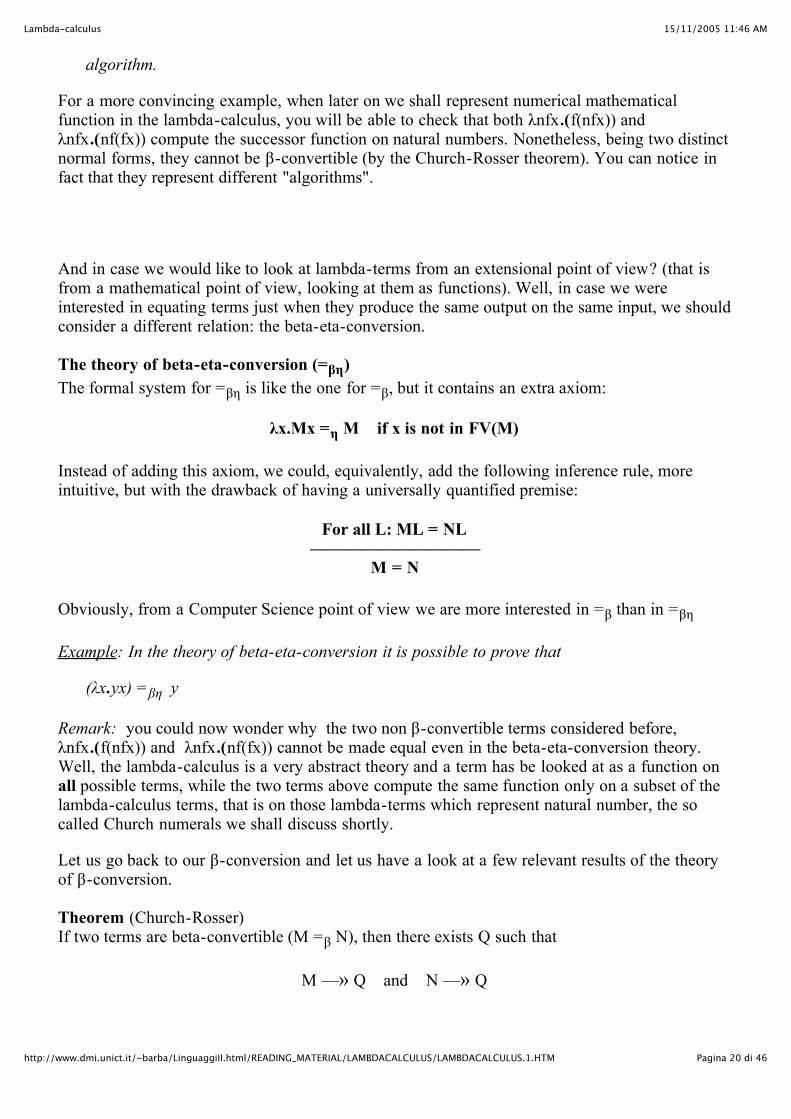
Instead of adding this axiom, we could, equivalently, add the following inference rule, moreintuitive, but with the drawback of having a universally quantified premise:
For all L: ML = NL——————————
M = N
Obviously, from a Computer Science point of view we are more interested in =β than in =βη
Example: In the theory of beta-eta-conversion it is possible to prove that
(λx.yx) =βη y
Remark: you could now wonder why the two non β-convertible terms considered before,λnfx.(f(nfx)) and λnfx.(nf(fx)) cannot be made equal even in the beta-eta-conversion theory.Well, the lambda-calculus is a very abstract theory and a term has be looked at as a function onall possible terms, while the two terms above compute the same function only on a subset of thelambda-calculus terms, that is on those lambda-terms which represent natural number, the socalled Church numerals we shall discuss shortly.
Let us go back to our β-conversion and let us have a look at a few relevant results of the theoryof β-conversion.
Theorem (Church-Rosser) If two terms are beta-convertible (M =β N), then there exists Q such that
M —» Q and N —» Q
The Church-Rosser theorem enables to prove that the theory of β-conversion is consistent. In a
15/11/2005 11:46 AMLambda-calculus
Pagina 21 di 46http://www.dmi.unict.it/~barba/LinguaggiII.html/READING_MATERIAL/LAMBDACALCULUS/LAMBDACALCULUS.1.HTM
The Church-Rosser theorem enables to prove that the theory of β-conversion is consistent. In alogic with negation, we say that a theory is consistent, if one cannot prove a proposition P andalso its negation P. In general, a theory is consistent if not all judgements are provable. Thanksto the Church-Rosser theorem, we can show that the λ-calculus is consistent.
Corollary (Consistency of =β) There exist at least two terms that are not β-convertible
Proof:Using the Church-Rosser theorem, we can prove:
(λx.yx) ≠β y
The two terms (λx.yx) and y are both in normal form. So, by the definition of β-conversion,they can be β-convertible only if
(λx.yx) ≡ y
But that is not the case, so they are not β-convertible.
The Church-Rosser theorem and the Confluence theorem are equivalent and in fact are often usedand referred to interchangedly:
The Church-Rosser theorem (C-R) and the Theorem of confluence (CONF) are logicallyequivalent, that is it is possible to prove one using the other
Proof:
C-R => CONF
Let us assume the Church-Rosser theorem and prove Confluence. In order to prove confluence let us take M, M1 and M2 such that
M —» M1 and M —» M2
By definition of β-conversion we have then that M1 =β M2. We can now use theChurch-Rosser theorem that guarantees that, whenever M1 =βM2, there exists L such that
M1 —» L and M2 —» L
CONF => C-R
Let us assume the Confluence theorem and prove the Church-Rosser one. We thenconsider two terms M and M' such that
M =β M'
By definition of beta-conversion, it means that I can transform M into M', by performingzero or more β-reductions / expansions:
15/11/2005 11:46 AMLambda-calculus
Pagina 22 di 46http://www.dmi.unict.it/~barba/LinguaggiII.html/READING_MATERIAL/LAMBDACALCULUS/LAMBDACALCULUS.1.HTM
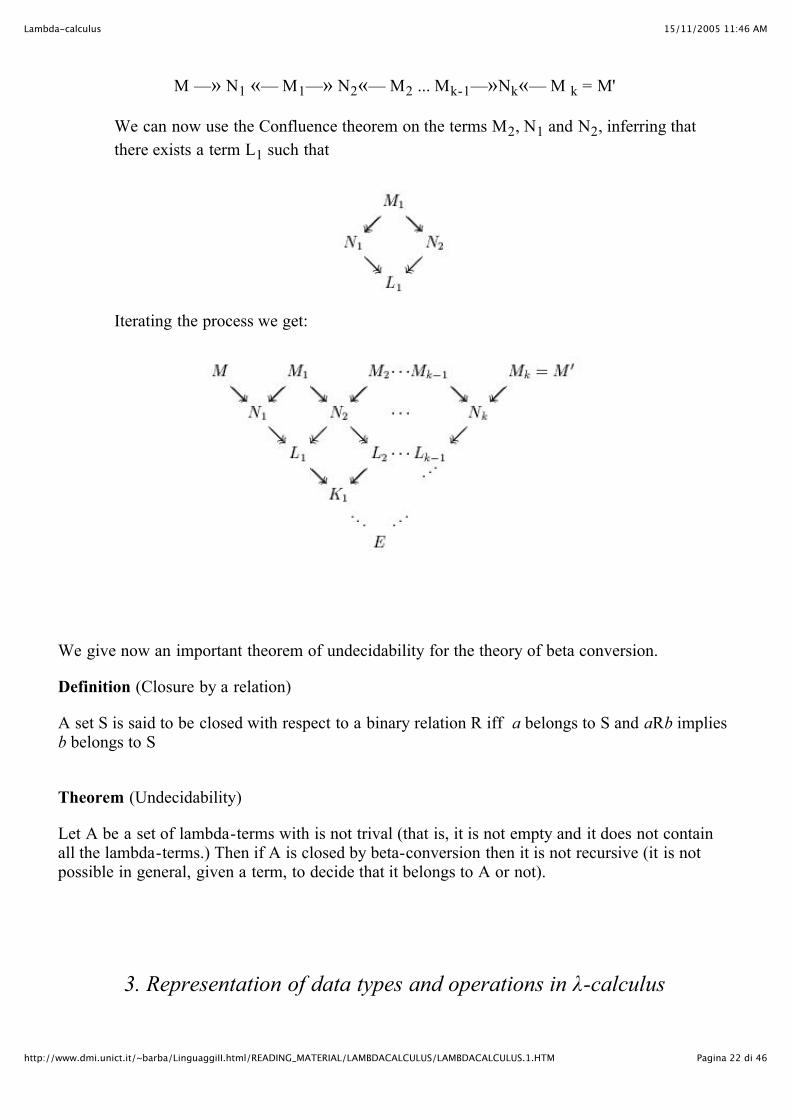
M —» N1 «— M1—» N2«— M2 ... Mk-1—»Nk«— M k = M'
We can now use the Confluence theorem on the terms M2, N1 and N2, inferring thatthere exists a term L1 such that
Iterating the process we get:
We give now an important theorem of undecidability for the theory of beta conversion.
Definition (Closure by a relation)
A set S is said to be closed with respect to a binary relation R iff a belongs to S and aRb impliesb belongs to S
Theorem (Undecidability)
Let A be a set of lambda-terms with is not trival (that is, it is not empty and it does not containall the lambda-terms.) Then if A is closed by beta-conversion then it is not recursive (it is notpossible in general, given a term, to decide that it belongs to A or not).
3. Representation of data types and operations in λ-calculus
15/11/2005 11:46 AMLambda-calculus
Pagina 23 di 46http://www.dmi.unict.it/~barba/LinguaggiII.html/READING_MATERIAL/LAMBDACALCULUS/LAMBDACALCULUS.1.HTM
3.1 The Natural numbers
In the syntax of the λ-calculus we have not considered primitive data types (the natural numbers,the booleans and so on), or primitive operations (addition, multiplication and so on), because theyindeed do not represent so primitive concepts. As a matter of fact we can represent them usingthe essential notions already contained in the λ-calculus, namely variable, application andabstraction.
The question now is: how can we represent in the λ-calculus a concept like that of naturalnumber?We stressed that the λ-calculus is a theory of functions as algorithms. This means that if we wishto represent natural numbers in the λ-calculus, we need to look at them as algorithms. How can itbe possible???? A number is a datum, not an algorithm! Well... but we could look at a numberas an algorithm. For instance, we could identify a natural number with the procedure we use to"build" it. Let us consider the number 2. How can we "build" it? Well, give me the successor,give me the zero and I can get the number 2 by iterating twice the successor function on thezero. How can I represent this procedure? By the lambda-term λfx. f (fx) !! Notice that the algorithm to build the number 2 is independent from what the zero and theconstructor actually are. We can abstract from what they actually are (fortunately, since nobodyreally knows what be zero and what be the successor. Do you?).
So, in general we can represent natural numbers as lambda-terms as follows
0 ≡ λfx. x (it represents the natural number 0) 1 ≡ λfx. f x (it represents the natural number 1) 2 ≡ λfx. f (f x) (it represents the natural number 2) 3 ≡ λfx. f (f (f x)) (it represents the natural number 3) ....................................................................................... n ≡ λfx. f nx (it represents the natural number n)
where we define f nx as follows: f 0x = x ; f k+1x = f(f kx) n denotes the lambda-representation of the number n.
The above encoding of the natural numbers is the original one developed by Church and theterms just defined are called Church's numerals. Church's encoding is just one among the manyone that it is possible to devise.
The technique to think of data as algorithms, can be extended to all the (inductively defined)data.
Example:
I can represent an unlabelled binary tree by the function that takes two inputs (the empty treeand the constructor that adds a root on top of two binary trees) and that returns as output theexpression that represents how to build the desired tree out of the emptytree and theconstructor.
15/11/2005 11:46 AMLambda-calculus
Pagina 24 di 46http://www.dmi.unict.it/~barba/LinguaggiII.html/READING_MATERIAL/LAMBDACALCULUS/LAMBDACALCULUS.1.HTM
In order to be sure that the representation of natural numbers we have given is a reasonable one,we have to show that it is also possible to represent in the lambda-calculus the operations onnumbers. But what does it means for a function on natural numbers to be definable in thelambda-calculus?
Definition (λ-definability) A function f: N → N is said to be λ-definible (representable in the λ-calculus) iff there exists aλ-term F such that:
F n =β f(n)
The term F is said to represent the function f.
Example:To represent the function factorial, we need to find a λ-term (let us call it fact) such that,whenever applied to the Church's numeral that represents the natural number n, we get aterm that is β-convertible to the Church's numeral representing the factorial of n, that is
fact 3 =β 6 Why have we not defined how to represent in the lambda-calculus the numerical functions withmore that one argument? Well, since it is enough to be able to represent their curryfied versions.So the definition given is enough.We shall see shortly how to define binary numerical functions like addition. What we shall do isto look at addition as AddCurr : N → (N → N)
Before seeing how to lambda-represent some numerical functions, let us see how we canrepresent the Booleans.
3.2 The Booleans
An encoding of the booleans corresponds to defining the terms true, false and if, satisfying (forall M and N):
if true M N = M if false M N = N
The following encoding is usually adopted:
true ≡ λxy.x false ≡ λxy.y if ≡ λpxy.pxy
Check that if actually works.
15/11/2005 11:46 AMLambda-calculus
Pagina 25 di 46http://www.dmi.unict.it/~barba/LinguaggiII.html/READING_MATERIAL/LAMBDACALCULUS/LAMBDACALCULUS.1.HTM
We have true ≠ false by the Church-Rosser theorem, since true and false are distinct normalforms. All the usual operations on truth values can be defined using the conditional operator.Here are negation, conjunction and disjunction:
and ≡ λpq. if p q false or ≡ λpq. if p true q not ≡ λp. if p false true
3.3 Arithmetic on Church's numerals
Using Church's encoding of natural numbers, addition, multiplication and exponentiation can bedefined very easily as follows:
add ≡ λmnfx.mf (nfx) mult ≡ λmnfx.m (nf) x expt ≡ λmnfx.nmfx
Addition is not hard to check. In fact:
add m n ≡ (λmnfx.mf (nfx)) m n →β (λnfx. m f (nfx)) n →β
→β λfx. m f (n f x) ≡ λfx.(λgx.gm x) f ((λhx.hn x) fx) →β
→β λfx.(λgx.gm x) f ((λx. f n x) x) →β λfx.(λgx.gm x) f (f n x) →β
→β λfx.(λx.f m x)(f n x) →β λfx.fm (f n x) ≡ λfx.f m+n x ≡ ≡ m+n
Multiplication is slightly more difficult:
mult m n ≡ (λmnfx.m(nf) x) m n →β (λnfx. m (nf) x) n →β
→β λfx. m (n f) x ≡ λfx.(λgx.gm x) (n f) x→β →β
→β λfx.(n f)m x → λfx.((λhx.hn x) f)m x →β λfx.(f n)m x ≡ λfx.f mx n x ≡ ≡ m x n
These reductions hold for all Church's numerals m and n,.
Here are other simple definitions:
succ ≡ λnfx. f (nfx) iszero ≡ λn.n (λx. false) true
The following reductions, as you can check by yourself, hold for any Church's numeral n:
succ n —» n+1 iszero 0 —» true iszero (n+1) —» false
15/11/2005 11:46 AMLambda-calculus
Pagina 26 di 46http://www.dmi.unict.it/~barba/LinguaggiII.html/READING_MATERIAL/LAMBDACALCULUS/LAMBDACALCULUS.1.HTM
iszero (n+1) —» false
Of course it is also possible to define the predecessor function (pred) in the lambda calculus, butwe do not do that here.
Now we can easily give the representation of the following mathematical function un naturalnumbers
f(n,m)=3+(m*5) if n=2 or n=0
(n+(3*m)) otherwise
by means of the following lambda-term:
λnm. if (or (iszero (pred (pred n))) (iszero n)) (add 3 (mult m 5)) (add n (mult 3 m))
3.4 Defining recursive functions using fixed points
In the syntax of the λ-calculus there is no primitive oparation that enables us to give names tolambda terms. However, that of giving names to expressions seems to be an essential features ofprogramming languages in order to define functions by recursion, like in Scheme
(define fact (lambda (x) (if (= x 0) 1 (* x (fact (- x 1))))))
or in Haskell
fact 0 = 1
fact n = n * fact (n-1)
Then, in order to define recursive functions, it would seem essential to be able to give names toexpressions, so that we can recursively refer to them.Surprisingly enough, however, that's not true at all. In fact, we can define recursive functions inthe lambda-calculus by using the few ingredients we have already at hand, exploiting the conceptof fixed point.
Definition Given a function f: A → A , a fixed point of f is an element a of A such that f (a) = a.
In the lambda-calculus, since we can look at any term M as a function from lambda-terms tolambda-terms, i.e. M : Λ → Λ, we can define a fixed point of M, if any, to be any term Qsuch that:
M Q =β Q
15/11/2005 11:46 AMLambda-calculus
Pagina 27 di 46http://www.dmi.unict.it/~barba/LinguaggiII.html/READING_MATERIAL/LAMBDACALCULUS/LAMBDACALCULUS.1.HTM
To see how we can fruitfully exploit the concept of fixed point, let us consider an example. Lesus take the definition of factorial using a generic sintax
factorial x = if (x=0) then 1 else x * factorial(x-1)
The above equation can be considered a definition because it identifies a precise function. Infact the function factorial is the only function which satisfies the following equation where fcan be looked at as an "unknown" function
f x = if x=0 then 1 else x * f(x-1)
The above equation can be rewritten as follows, by using the lambda notation
f =λx. if x=0 then 1 else x * f(x-1)
The function we are defining is hence a fixpoint, the fixpoint of the functional
λf.λx. if x=0 then 1 else x * f(x-1)
In fact it can be checked that
(λf.λx. if x=0 then 1 else x * f(x-1)) factorial = factorial
Now, we want to lambda-represent the factorial function. It is easy to see that the functional
λf.λx. if x=0 then 1 else x * f(x-1)
can be easily lambda-represented:
λ f.λx.if (iszero x) 1 (mult (f(sub x 1)) x)
Then, a lambda term F that lambda-represents the factorial function must be a fixed point ofthe above term. Such an F would in fact satisfy the following equation
F x =β if (iszero x) 1 (mult x (F(sub x 1)))
and hence would be really the lambda-representation of the factorial.
But is it possible to find fixed points of lambda-terms? And for which lambda-terms? Well, thefollowing theorem settles the question once and for all, by showing us that all lambda-termsindeed have a fixed point. Moreover, in the proof of the theorem it will be shown how easy it ispossible to find a fixed point for a lambda term.
Theorem Any λ-term has at least one fixed point.
Proof.We prove the theorem by showing that there exist lambda terms (called fixed point operators)which,
15/11/2005 11:46 AMLambda-calculus
Pagina 28 di 46http://www.dmi.unict.it/~barba/LinguaggiII.html/READING_MATERIAL/LAMBDACALCULUS/LAMBDACALCULUS.1.HTM
which,given an arbitrary lambda term, produce a fixed point of its. One of those operators (combinators) is the combinator Y discovered by Haskell B. Curry.It is defined as follows:
Y ≡ λf. (λx. f(xx)) (λx. f(xx))
It is easy to prove that Y is a fixed point combinator. Let F be an arbitrary λ-term. We have that
Y F → (λf. (λx. f(xx)) (λx. f(xx))) F → (λx. F(xx)) (λx. F(xx)) →
→ F ((λx. F(xx)) (λx. F(xx))) → (3)
= F (Y F)
That is
F (Y F) =β (Y F)
Then the λ-term that represents the factorial function is:
Y(λf.λx.if (iszero x) 1 (mult x (f(sub x 1))))
Let us consider another example of recursively defined function.
g x = if (x=2) then 2 else g x (*) What is the function defined by this equation? Well, it is the function that satisfies the equation,where g is considered an "unknown" function.
Ok, but we have a problem here, since it is possible to show that there are many functions thatsatisfy this equation. In fact, it is easy to check that
factorial x = if (x=2) then 2 else factorial x
And also the identity function satisfies the equation, sknce
identity x = if (x=2) then 2 else identity x
And many more. For instance, let us consider the function gee that returns 2 when x=2 and that isundefined otherwise. Well, also gee satisfies the equation:
gee x = if (x=2) then 2 else gee x
So, which one among all the possible solutions of (*), that is which one among all the possiblefixed point of the functorial
15/11/2005 11:46 AMLambda-calculus
Pagina 29 di 46http://www.dmi.unict.it/~barba/LinguaggiII.html/READING_MATERIAL/LAMBDACALCULUS/LAMBDACALCULUS.1.HTM
λg.λx. if x=2 then 2 else g x
do we have to consider as the function identified by the definition (*). We all know that it is gee the intended function defined by (*). Why? Because implicitely, when we give a definition like (*), we are considering a computationalprocess that identifies the least among all the possible solutions of the equation (least in the senseof "the least defined"). This means that, in order to correctly lambda-define the functionidentified by an equation like (*), we cannot consider any fixed point, but the least fixed point(the one that corresponds to the least defined function that respects the equation.)
The question now is: does the Y combinator picks the right fixed point? If a lambda term hasmore than one fixed point, which is the one picked up Y? Well, Y is really a great guy. It not only returns a fixed point of a term, but the least fixed point,where informally for least we mean the one that contains only the information strictly needed inorder to be a fixed point. Of course we could be more precise in what we mean by a term "havingless information" than another one and in what we mean by least fixed-point, but we would gobeyond the scope of out introductory notes.
It is enough for us to know that the least fixed point of the functional
λf. λx. if iszero (pred (pred x)) 2 (f x) and hence the lambda term lambda-representing the function gee is
Y(λf. λx. if iszero (pred (pred x)) 2 (f x))
Let us look at some other easy exampleExample:
Let us consider the λ-term:
λx.xAny other term M is a fixed point of λx.x (the function identity) because:
λx.x =β M
The least fixed point, between all the ones fixed points of λx.x, is Ω (intuitively you can seethat this is the term that has no information at all in it). IWe can check that
Y (λx.x) = Ω
Example:Let us consider, now, a function indefinite in all the domain, that is the one define by theequation:
h x = h xThe λ-term that represents that, is the solution of the equation:
h = λx. h xThat is the least fixed point of:
15/11/2005 11:46 AMLambda-calculus
Pagina 30 di 46http://www.dmi.unict.it/~barba/LinguaggiII.html/READING_MATERIAL/LAMBDACALCULUS/LAMBDACALCULUS.1.HTM
λf. λx. f x
the least fixed point of this term is the function indefinite in every value.
If we consider the (3), there we have two β-reductions (the first two), then a β-expansion. Itmeans that it's impossible to have:
Y F —» F (Y F)
There is another fixed point combinator: Alan Turing's Θ:
A ≡ λxy.y (xxy) Θ ≡ AA
Its peculiarity is that we have that
Θ F —» F (Θ F)
Then I can get the relation above, using only β-reductions.
The Why of Y.
Let us see intuitively noy why the combinator Y (and the fixed point combinators in general)works.
Let us consider once again the factorial function
factorial x = if (x=0) then 1 else x * factorial(x-1)
You see, in a sense this definition is equivalent to
factorial x = if (x=0) then 1 else x * ( if (x-1=0) then 1 else (x-1) * factorial(x-1-1) )
and also to
factorial x = if (x=0) then 1 else x * (if (x-1=0) then 1 else (x-1) * (if (x-1-1=0) then 1 else (x-1-1) * factorial(x-1-1-1) ) )
and so on....
To compute the factorial, in a sense, we unwind its definition as many times as it is needed bythe argument, that is until x-1-1-1...-1 gets equal to 0. That is exactly what the Y combinatordoes, in fact
Y F =β F(Y F) =β F(F(Y F)) =β F(F(F(Y F))) =β F(F(F(F(Y F)))) =β ... and so on
15/11/2005 11:46 AMLambda-calculus
Pagina 31 di 46http://www.dmi.unict.it/~barba/LinguaggiII.html/READING_MATERIAL/LAMBDACALCULUS/LAMBDACALCULUS.1.HTM
If you take as F the lambda term λf.λx.if (iszero x) 1 (mult x (f (sub x 1))) , by applying a beta-reduction you get
Y F =β λx.if (iszero x) 1 (mult x ((Y F)(sub x 1)))
but you can also get
Y F =β λx.if (iszero x) 1 (mult x ((if (iszero (sub x 1)) 1 (mult (sub x 1) ((Y F)(sub (sub x 1) 1)))
and so and so on
That is (Y F) is beta-convertible to all the possible "unwindings" of the factorial definition. Thenif you apply 2 to (Y F) you can get, by a few beta-reduction
(Y F)2 =β if (iszero 2) 1 (mult 2 ((if (iszero (sub 2 1)) 1 (mult (sub 2 1) (if (iszero (sub (sub x1) 1)) 1 (mult (sub (sub x 1) 1) ((Y F)(sub (sub (sub x 1) 1) 1)))))
you can now easily see that the right term is beta convertible to 2 that is the factorial of 2.
Then, why Y works? Because, in a sense, it is an "unwinder", an "unroller" of definitions.
Using Y (and hence recursion) to define infinite objects.
In lambda calculus it is easy to represent also the data type List. In fact it is possible to representthe empty list and the operators of list (we do not give here their precise representation).
Let us consider now the following λ-term:
Y (λl. cons x l) (*)
It represent a fixed point. We used Y before to represent recursively defined function in lambda-calculus, but it is not the only way to use Y. Here we use it to represent the fixed-point of thefunction λl. cons x l, whose fixed point, you can check is an infinite list, the infinite list of x's.This means that the term Y (λl. cons x l) indeed represent an infinite object!Of course we cannot completely evaluate this term (i.e. get all the information it contains), sincethe value of this term would be an infinitely long term in normal form, but we can evaluate it inorder to get all possible finite approximation of the infinite list of x's.You see, after a few beta reductions and beta conversions you can obtain:
(cons x (cons x ( cons x (Y F)))) where F represents the term (*)
and this term is a finite approximation of the infinite list of x's. Of course the term (*) isconvertible to all the possible finite approximations of the infinite list of x's. This means that it ispossible to use and work with terms representing infinite object. In fact let us consider
car (Y (λl. cons x l)) =β x (**)
where car is the λ-representation of the function that, taken a list, returns its first element. Wecan see thatit is possible manipulate the term (*), even if it represent an infinite object. This possibility show
15/11/2005 11:46 AMLambda-calculus
Pagina 32 di 46http://www.dmi.unict.it/~barba/LinguaggiII.html/READING_MATERIAL/LAMBDACALCULUS/LAMBDACALCULUS.1.HTM
it is possible manipulate the term (*), even if it represent an infinite object. This possibility showthat in functional programming it is possible to deal also with infinite objects. This possibility,however is not present in all functional languages, since to evaluate an expression in a functionallanguage we precise reduction strategies, and not all the reduction strategies enable to handleinfinite objects. In Scheme it is not possible since, in a term like (**) above Sheme would keepon evaluating the argument of the car, going on to the infinite. In Haskell instead, the evaluationof a term like (**) terminates.In order to better understand this fact, see the section below on evaluation strategies.
3.5 Reduction strategies
One of the aspects that characterizes a functional programming language is the reduction strategyit uses Let us define such notion in the lambda-calculus.
Definition A reduction strategy is a "policy" that, given a term, permits to choose a β-redex among all thepossible ones present in the term. Abstractly, we can consider a strategy like a function
S: Λ → Λ
(where Λ is the set of all the λ-terms), such that:
if S(M) = N then M →β N
(M reduces to N in one step). Let us see, now, same classes of strategy.
Call-by-value strategies
These are all the strategies that never reduce a redex when the argument is not a value (that is,when we can still reduce the argument). OF course we need to precisely formalize what weintend for "value".In the following example we consider a value to be a lambda term in normal form.
Example:Let us suppose to have:
((λx.x)((λy.y) z)) ((λx.x)((λy.y) z))
A call-by-value strategy never reduce the term (λx.x)((λy.y) z) because the argument it is nota value. In a call-by-value strategy, then, I reduce only one of the redex underlined.
Scheme uses a specific call-by-value strategy, and a particular notion of value. Informally, up to now we have considered as "values" the terms in normal form. For Scheme,instead, also a function is considered to be a value (an expression like λx.M, in Scheme, is avalue). Then, if I have:
15/11/2005 11:46 AMLambda-calculus
Pagina 33 di 46http://www.dmi.unict.it/~barba/LinguaggiII.html/READING_MATERIAL/LAMBDACALCULUS/LAMBDACALCULUS.1.HTM
(λx.x) (λz.(λx.x) x)
Scheme's reduction strategy considers the biggest redex (all the term), reduces it and then stopsbecause it get something that is a value for Scheme (for Scheme the term λz.((λx.x) x) is a valueand hence it is left as it is by the interpreter.).
Call-by-name strategies
These are all the strategies that reduce a redex without checking whether its argument is a valueor not. One of its subclasses is the set of lazy strategies. Generally, in programming languages astrategy is lazy if it is call-by-name and reduces a redex only if it's strictly necessary to get thefinal value (this strategy is called call-by-need too). One possible strategy call-by-name is theleftmost-outermost one: it takes, in the set of the possible redex, the leftmost and outermost one.
Example:Let us denote by I the identity function and let us consider the term:
(I (II)) ( I (II))
the leftmost-outermost strategy first reduces the underlined redex.
This strategy is very important because if a term has a normal form, it finds that. The problem isthat the number of reduction steps is sometimes greater then the strictly necessary ones.
If a language uses a call-by-value strategy, we have to be careful because if an expression hasnot normal form, the search could go ahead to the infinite.
Example:Let us consider the functional F that has the factorial function as fixed point. Then, we cansay that:
(Θ F) 3 —» 6Let us suppose to use a call-by-value strategy. I get:
(Θ F) 3 → (F (Θ F)) 3 → (F (F (Θ F))) 3 → ...If we would like to use the above fixed point operator to define recursive function in Scheme (wedo not do that when we program in Scheme, of course), we have this problem. We could overcome this problem, however, by defining a new fixed point combinator, H, that Icould use in Scheme and any aty I have a reduction strategy like that used by Scheme. Let usconsider the following λ-term:
H = λg.((λf.ff) (λf.(gλx.ffx)))
It's easy to prove that this term is a fixed point operator. In fact we have that:
(H F) —» F (λx. AAx)
15/11/2005 11:46 AMLambda-calculus
Pagina 34 di 46http://www.dmi.unict.it/~barba/LinguaggiII.html/READING_MATERIAL/LAMBDACALCULUS/LAMBDACALCULUS.1.HTM
where A is (λf.F λx.ffx) and (HF) —» AA. From the point of view of the computations, we canwrite it in this form:
(H F) —» F (λx. H Fx)
Functionally, F (λx. H Fx) has the same behaviour of HF, but scheme does not reduce it becausethat's a value for scheme. Then if, for example, F is the functional whose fixed-point representsthe function factorial, in order to compute fact 5 we have to evaluate the term ((HF)5).That is wehave to evaluate
(F (λx. H Fx)) 5
and this evaluation is possible withouth getting an an infinite reduction sequence.
3.6 Head Normal Form
In the previous sections, we have implicitly assumed that in λ-calculus if a term has not a normalform, then it represents no information at all. For example:
Ω has not normal form and it represents the indefinite value
But this is not always true, that is it is possible to have terms that have no normal form butnonetheless represent ("contain") some information. Let us consider the following λ-term:
Y (λl. cons x l) (*)
which represents the infinite list of x's. We cannot completely evaluate this term (i.e. get all theinformation it contains), since the value of this term would be an infinitely long term in normalform. The term above does not have a normal form but nonetheless it has a "meaning" (the infinite listof x´s). In fact after some β-reductions I can get a finite approximation of its "meaning". Youcan see that after a few beta reductions we can obtain:
(cons x (cons x ( cons x (Y F)))) where F represents the term (*)
and this term is a finite approximation of the infinite list of x's.
It is possible to use and work with terms that have no normal form but nonetheless posses a"meaning. In fact, let us consider:
hd (Y (λl. cons x l)) —» x
where hd is the λ-representation of the function that, taken a list, returns its first element. We cansee thatit is possible manipulate the term (*), even if it represent an infinite object.
15/11/2005 11:46 AMLambda-calculus
Pagina 35 di 46http://www.dmi.unict.it/~barba/LinguaggiII.html/READING_MATERIAL/LAMBDACALCULUS/LAMBDACALCULUS.1.HTM
Note:In this case, I have to be careful about the strategy I intend to use. If I use a call-by-valuestrategy, where I consider as values the terms in normal form, I get an infinite chain of β-reductions where in every step I reduce the subterm
Y (λl. cons x l)
In a language like Haskell, instead, I obtain x (When you begin to have a look at Haskell,read also the notes [HASK] on laziness and infinite objects, available in the readingmaterial)
How it is possible to formalize in lambda-calculus the notion we have informally discussedabove? that is, the notion of a term that contains some information even if it could also have nonormal form.We do that by introducing the concept of head normal form, representing the notion of finiteapproximation of the meaning of a term.
Definition A term is in head normal form (hnf) if, and only if, it looks like this:
λx1...xk.yM1...Mn (n,k≥ 0)
where y can be any variable, also one of the xi's. If this term had normal form, that it will be of the form:
λx1...xk.yN1...Nn
where N1,...,Nn would be the normal form of M1,...,Mn. Instead, if the term had no normal form,I'm sure that in any case the portion of the term
λx1...xk.y
will stay always the same in any possible reduction sequence.(Let us note that a term in normal form is also in head normal form).
Example:Let us consider the term:
λxyz.z(λx.x)(λzt.t(zz))(λt.t(λ (λxx)))
it is in normal form, but it is in head normal form too.
Let us consider, now, Ω. It is not in head normal form and it has no head normal form.
Now, going back to the notion of term containing no information (term representing theindeterminate), we have just seen that some information can be contained also in terms having nonormal form. So when can I say that a term contain no information? Well, now we can answer:when a term has no head normal form!Are we sure this to be the right answer? Well, the following fact confirms that it is really theright answer:
15/11/2005 11:46 AMLambda-calculus
Pagina 36 di 46http://www.dmi.unict.it/~barba/LinguaggiII.html/READING_MATERIAL/LAMBDACALCULUS/LAMBDACALCULUS.1.HTM
right answer:Let us take two terms not having head normal form, for example:
Ω and Ωx
Using Church-Rosser theorem I can prove they are not β-convertible. Now If I add to the β-conversion theory the axiom:
Ω = β Ωx
the theory of beta-conversion does remain consistent. It is no surprise, since this axiom is statingthat a term that contains no information is equivalent to a term that contains no information, nocontradiction in that!Then, we can rightly represent the indeterminate with any term that has not head normal form. Indeed I could consistently add to the theory of the beta-conversion the axiom stating that all theterms with no head normal form are β-convertible (pratically we could consistently "collapse" allthe possible representations of the indeterminate into one element).
4. Types
4.1 Introduction to types
The functional programming languages can be typed or not typed. A typed one is, for example,Haskell, while one not typed is Scheme. Let us introduce the concept of type in λ-calculus. Wecan look at types as predicates on programs or, better, as partial specifications about thebehaviour of a program. By means of types a number of programming errors can be prevented.
There are two different approach to the use of types.
the approach a' la Curry (the one used in Haskell)the approach a' la Church (the one used in Pascal)
In the Curry approach, I usually first write a program and then I check whether it satisfies aspecification. Instead, in the Church approach the types are included in the syntax of the language and, in asense, represent some constraints I have to follow during the writing of my code (they prevent meto write wrong terms).In the approach a' la Curry, checking if a term M satisfies a specification represented by a type t, it is usually referred to as "assigning the type t to the term M".
4.2 Type assignment 'a la Curry
In this approach we write a program and then we check if the program satisfies the specificationhe have in mind for it. It means that we have two distinct sets: programs and partialspecifications. If we wish to talk in a general and abstract way about types (a' la Curry) in functionalprogramming languages we can proceed with the following formalization:
15/11/2005 11:46 AMLambda-calculus
Pagina 37 di 46http://www.dmi.unict.it/~barba/LinguaggiII.html/READING_MATERIAL/LAMBDACALCULUS/LAMBDACALCULUS.1.HTM
programming languages we can proceed with the following formalization:
Programs : the set of λ-terms, i.e. / Partial specifications: the set of types, i.e.Λ T ::= φ | T → T
where φ is a meta-variable which value is defined over a set of type variables (φ, φ', φ'', a, b, ...etc.). In this formalization we have considered the simplest form of type (in fact this types arecalled "simple types"). Elements of T in general will be denoted by σ, τ , ρ, etc.
There are now a whole bunch of questions we would like to answer:
1) How can I formally show that, given a program (a term) M and a specification (a type) σ,M satisfies the specification σ, that is that M has type σ?
2) Is it decidable, given a M and a σ, that M is of type σ?
3) Do types play any role during a computation?
4) Is it possible to "compare" types, that is to formalize the notion that a type is "moregeneral" than another one?
5) What is the intrinsic meaning of having type variables in our system? has the use of typevariable some implication for our system?
6) Is it possible that among all the possible types I can give to a term M, there exists the mostgeneral one? If so, can it be algorithmically found?
Let us start with question 1). So, what we need to do is to device a formal system whose judgments are of the form
M : σ
whose meaning is: the program M respects the specification σ (the term M has type σ).
Thinking about it better, however, the judgments we need should be a bit richer that simply M : σ. In fact, let us consider the term λx.yx. It is possible to infer that this terms has type, for instance:
φ → something
But how can we determine what something is if we do not have any information about the freevariable y?This means that the (typing) judgments we are looking for need to be of the shape:
B |—M:σ
where B provide informations about the free variables of M. The meaning of B |— M : σ is then"using the informations given by the basis B, the term M has type σ" (M has type σ in the basisB).The basis B contains informations about the types of the free variables of M.
15/11/2005 11:46 AMLambda-calculus
Pagina 38 di 46http://www.dmi.unict.it/~barba/LinguaggiII.html/READING_MATERIAL/LAMBDACALCULUS/LAMBDACALCULUS.1.HTM
The basis B contains informations about the types of the free variables of M.Formally B will be a set of pairs of the form : variable : type
Example:One example of basis is:
B = x : τ , z : ρ
Let us introduce now the formal system.
Definition (Curry type assignment system)
Axiom—————
B |— x : σ if x : σ is in B
(a variable x has type σ if the statement x : σ is in B).
Inference rules
These rules allow to derive all the possible valid typing judgements.
B |— M : σ → τ B |— N : σ———————————————
B |— MN : τ
This rule says that if, using the assumptions in B, I can prove that M has type σ → τ and Nhas type σ, then I can prove that in the basis B the application MN has type τ. This rule isusually called (→E): "arrow elimination". Of course this rule can be "read" also bottom-up,that is: if we wish to prove that MN has type τ in B, then we need to prove that M has type σ → τ in B for some σ and that N has type σ in B.
B, x : σ |— M : τ
————————— B |— λx.M : σ → τ
This rule says that if, using the assumptions in B and the further assumption "x has type σ", I can prove that M has type τ, then I can prove that in B λx.M has type σ → τ. Thisrule is called (→I) : "arrow introduction". Also this rule can be "read" bottom-up. Do it asexercise.
We remark that the above formal system is the core of the type systems of languages likeHaskell, ML and others. This is the main motivation for which we are studying it.
15/11/2005 11:46 AMLambda-calculus
Pagina 39 di 46http://www.dmi.unict.it/~barba/LinguaggiII.html/READING_MATERIAL/LAMBDACALCULUS/LAMBDACALCULUS.1.HTM
Haskell, ML and others. This is the main motivation for which we are studying it.
Example:
In Haskell, before the definition of a function, I can declare what type the function isintended to have:
fact :: Int → Int
Once I have defined the function fact, the Haskell interpreter checks if the program satisfiesthe specification I had given, that is it tries to derive, in a formal system like the one seenbefore, a typing judgement. Note: In Haskell we have not the concept of basis, because all correct programs have to beclosed expressions (without free variables). That is, better, all the free variables in a programmust have been associated previously to some value.
Example:
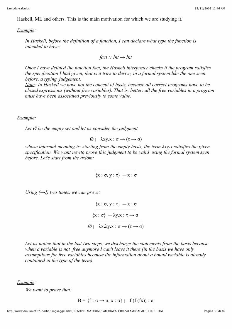
Let Ø be the empty set and let us consider the judgment
Ø |— λxy.x : σ → (τ → σ)whose informal meaning is: starting from the empty basis, the term λxy.x satisfies the givenspecification. We want nowto prove this judgment to be valid using the formal system seenbefore. Let's start from the axiom:
————————x : σ, y : τ |— x : σ
Using (→I) two times, we can prove:
x : σ, y : τ |— x : σ————————
x : σ |— λy.x : τ → σ ——————————— Ø |— λx.λy.x : σ → (τ → σ)
Let us notice that in the last two steps, we discharge the statements from the basis becausewhen a variable is not free anymore I can't leave it there (in the basis we have onlyassumptions for free variables because the information about a bound variable is alreadycontained in the type of the term).
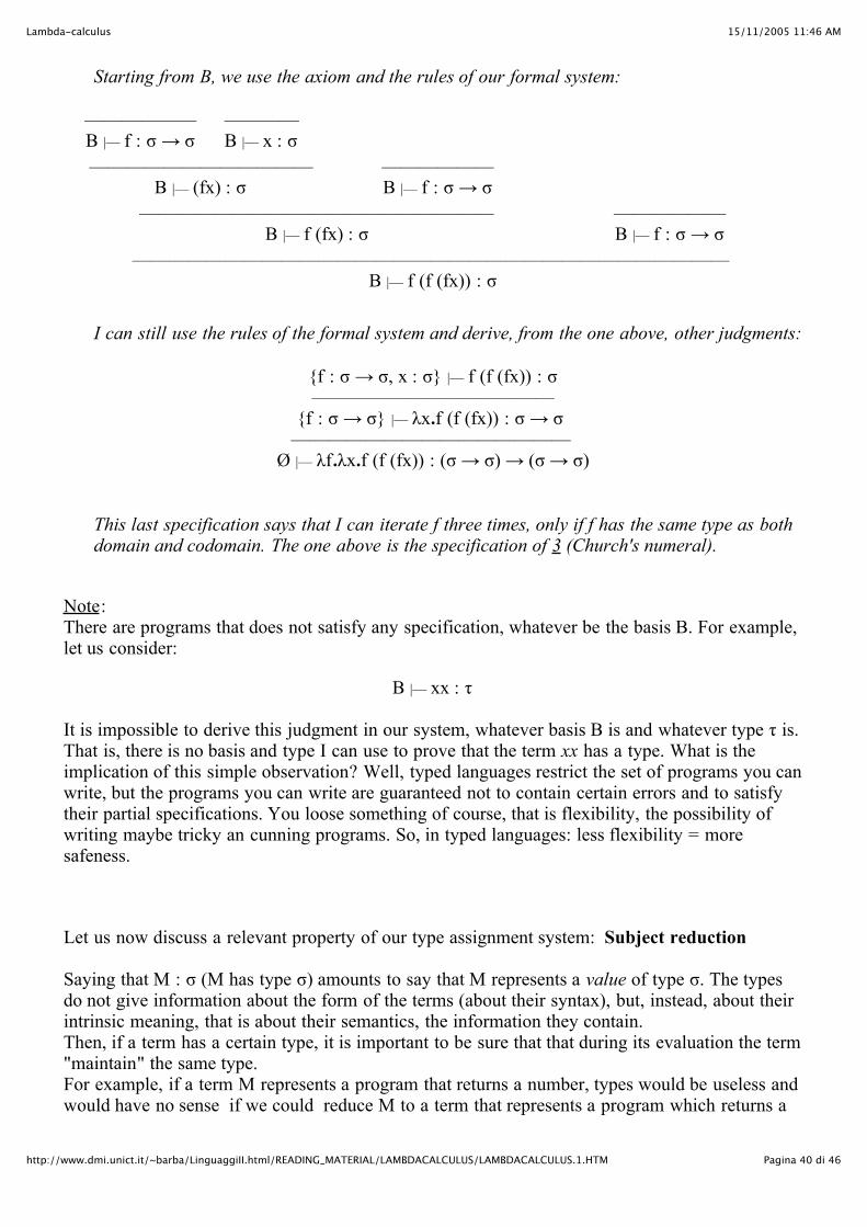
Example:We want to prove that:
B = f : σ → σ, x : σ |— f (f (fx)) : σ
15/11/2005 11:46 AMLambda-calculus
Pagina 40 di 46http://www.dmi.unict.it/~barba/LinguaggiII.html/READING_MATERIAL/LAMBDACALCULUS/LAMBDACALCULUS.1.HTM
Starting from B, we use the axiom and the rules of our formal system:
——————B |— f : σ → σ
————B |— x : σ
————————————B |— (fx) : σ
——————B |— f : σ → σ
———————————————————B |— f (fx) : σ
——————B |— f : σ → σ
———————————————————————————————— B |— f (f (fx)) : σ
I can still use the rules of the formal system and derive, from the one above, other judgments:
f : σ → σ, x : σ |— f (f (fx)) : σ—————————————
f : σ → σ |— λx.f (f (fx)) : σ → σ ———————————————
Ø |— λf.λx.f (f (fx)) : (σ → σ) → (σ → σ)
This last specification says that I can iterate f three times, only if f has the same type as bothdomain and codomain. The one above is the specification of 3 (Church's numeral).
Note: There are programs that does not satisfy any specification, whatever be the basis B. For example,let us consider:
B |— xx : τ
It is impossible to derive this judgment in our system, whatever basis B is and whatever type τ is.That is, there is no basis and type I can use to prove that the term xx has a type. What is theimplication of this simple observation? Well, typed languages restrict the set of programs you canwrite, but the programs you can write are guaranteed not to contain certain errors and to satisfytheir partial specifications. You loose something of course, that is flexibility, the possibility ofwriting maybe tricky an cunning programs. So, in typed languages: less flexibility = moresafeness.
Let us now discuss a relevant property of our type assignment system: Subject reduction
Saying that M : σ (M has type σ) amounts to say that M represents a value of type σ. The typesdo not give information about the form of the terms (about their syntax), but, instead, about theirintrinsic meaning, that is about their semantics, the information they contain. Then, if a term has a certain type, it is important to be sure that that during its evaluation the term"maintain" the same type.For example, if a term M represents a program that returns a number, types would be useless andwould have no sense if we could reduce M to a term that represents a program which returns alist.
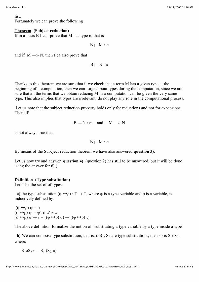
15/11/2005 11:46 AMLambda-calculus
Pagina 41 di 46http://www.dmi.unict.it/~barba/LinguaggiII.html/READING_MATERIAL/LAMBDACALCULUS/LAMBDACALCULUS.1.HTM
list. Fortunately we can prove the following
Theorem (Subject reduction)If in a basis B I can prove that M has type σ, that is
B |— M : σ
and if M —» N, then I ca also prove that
B |— N : σ
Thanks to this theorem we are sure that if we check that a term M has a given type at thebeginning of a computation, then we can forget about types during the computation, since we aresure that all the terms that we obtain reducing M in a computation can be given the very sametype. This also implies that types are irrelevant, do not play any role in the computational process.
Let us note that the subject reduction property holds only for reductions and not for expansions.Then, if:
B |— N : σ and M —» N
is not always true that:
B |— M : σ By means of the Subcject reduction theorem we have also answered question 3).
Let us now try and answer question 4). (question 2) has still to be answered, but it will be doneusing the answer for 6) )
Definition (Type substitution)Let T be the set of of types:
a) the type substitution (φ ρ) : T → T, where φ is a type-variable and ρ is a variable, isinductively defined by:
(φ ρ) φ = ρ (φ ρ) φ' = φ', if φ' ≠ φ (φ ρ) σ → τ = ((φ ρ) σ) → ((φ ρ) τ)
The above definition formalize the notion of "substituting a type variable by a type inside a type"
b) We can compose type substitution, that is, if S1, S2 are type substitutions, then so is S1oS2,where:
S1oS2 σ = S1 (S2 σ)
15/11/2005 11:46 AMLambda-calculus
Pagina 42 di 46http://www.dmi.unict.it/~barba/LinguaggiII.html/READING_MATERIAL/LAMBDACALCULUS/LAMBDACALCULUS.1.HTM
c) A type substitution can also be applied to a basis: SB = x : Sτ | x : τ is in B
d) A type substitution can also be applied to pairs of basis and type (it will be useful later on)
S <B, σ> = <SB, Sσ>
Example: if we apply the type substitution (φ σ) to the type φ → (τ→ φ), we obtain thetype σ → (τ→ σ)
- If for σ,τ there is a substitution S such that Sσ = τ, then τ is a (substitution) instance of σ.
We answer to question 2) above by giving the following definition.
Definition (more general type)Given two types τ and σ, τ is more general than σ if the latter can be obtained from the former bymeans of a type substitution, i.e. if there exists S such that τ = S(σ).
The following lemma show that if we can give a type to a term, we can give infinitely many andindeed it will provide an answer also to question 5).
Lemma (substitution lemma) If starting from a basis B we can prove that M has type σ, that is
B |— M : σ
then, for all possible substitutions S, we can also prove that:
S(B) |— M : S(σ)
Example:It's easy to prove that:
x : φ → ψ |— λy .xy : φ → ψThe lemma above says that if I apply any substitution S, I can prove that:
S(x : φ → ψ) |— λy .xy : S(φ → ψ)For example, if I consider the following substitution:
(φ (φ' → φ)) o (ψ ξ)then it is possible to prove that:
x : (φ' → φ) → ξ |— (λy .xy) : (φ' → φ) → ξ
So if a term satisfies a specification, then it satisfies infinitely many ones because we can haveinfinite possible substitutions.
15/11/2005 11:46 AMLambda-calculus
Pagina 43 di 46http://www.dmi.unict.it/~barba/LinguaggiII.html/READING_MATERIAL/LAMBDACALCULUS/LAMBDACALCULUS.1.HTM
infinite possible substitutions.
Example:If we have derived
Ø |— λx.x : φ → φby the lemma of substitution I am also sure that also the following is derivable
Ø |— λx.x : (ψ → φ) → (ψ → φ)
But there are infinite substitutions that I can apply, so if a term satisfies a specification, itsatisfies infinite specifications.
What we have just seen means that in our formal system we have polymorphic functions (afunction is called polymorphic if it can be correctly applied to objects of different types).So, by using type variables, we have implicitly introduced a notion of polymorphism in our typeassignment system.Since this system is the core of the type system of Haskell this implies that Haskell is a languagewith polimorphism. (In Haskell type variables have names like a, b, c etc.)
The polymorphism of our system can be said to be implicit, since the fact that a term has moretypes it is not explicitly expressed in the syntax but it is expressed by results like the substitutionlemma. One example of a syntax for explicit polymorphism could be the following:
λx.x : for all φ.φ → φ
In this case the polymorphic behaviour of the term is explicitely described by the sintax.
We have just said that if I have a term M, it has infinite specifications. It is possible to prove thatexists a relation among all the types that a given term can have (i.e. all the possible partialspecifications of a program are connected). We are then trying to give an answer to question 6).The answer will also provide an answer to question 2) that we had left unanswered.
4.3 Principal pairs
Theorem Given a term M, if M is typeable then it has a Principal Pair <P, π>, where P is a basis and π atype such that:
1) I can derive the following typing for M
P |— M : π
2) the principal pair represents the most generic typing possible for M. That is, I can get anyother basis and type from that. It means that if:
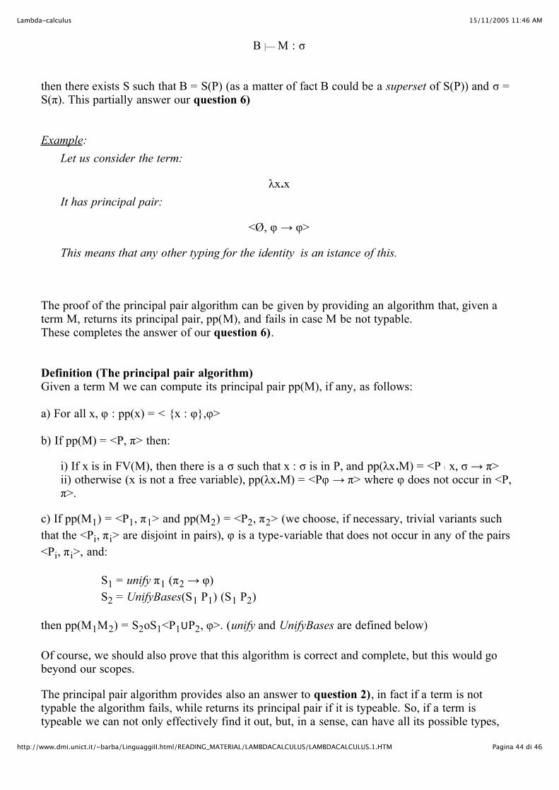
15/11/2005 11:46 AMLambda-calculus
Pagina 44 di 46http://www.dmi.unict.it/~barba/LinguaggiII.html/READING_MATERIAL/LAMBDACALCULUS/LAMBDACALCULUS.1.HTM
B |— M : σ
then there exists S such that B = S(P) (as a matter of fact B could be a superset of S(P)) and σ =S(π). This partially answer our question 6)
Example:Let us consider the term:
λx.xIt has principal pair:
<Ø, φ → φ>
This means that any other typing for the identity is an istance of this.
The proof of the principal pair algorithm can be given by providing an algorithm that, given aterm M, returns its principal pair, pp(M), and fails in case M be not typable.These completes the answer of our question 6).
Definition (The principal pair algorithm)Given a term M we can compute its principal pair pp(M), if any, as follows:
a) For all x, φ : pp(x) = < x : φ,φ>
b) If pp(M) = <P, π> then:
i) If x is in FV(M), then there is a σ such that x : σ is in P, and pp(λx.M) = <P \ x, σ → π> ii) otherwise (x is not a free variable), pp(λx.M) = <Pφ → π> where φ does not occur in <P, π>.
c) If pp(M1) = <P1, π1> and pp(M2) = <P2, π2> (we choose, if necessary, trivial variants suchthat the <Pi, πi> are disjoint in pairs), φ is a type-variable that does not occur in any of the pairs<Pi, πi>, and:
S1 = unify π1 (π2 → φ) S2 = UnifyBases(S1 P1) (S1 P2)
then pp(M1M2) = S2oS1<P1UP2, φ>. (unify and UnifyBases are defined below)
Of course, we should also prove that this algorithm is correct and complete, but this would gobeyond our scopes.
The principal pair algorithm provides also an answer to question 2), in fact if a term is nottypable the algorithm fails, while returns its principal pair if it is typeable. So, if a term istypeable we can not only effectively find it out, but, in a sense, can have all its possible types,since any possible typing can be got out of the principal pair.
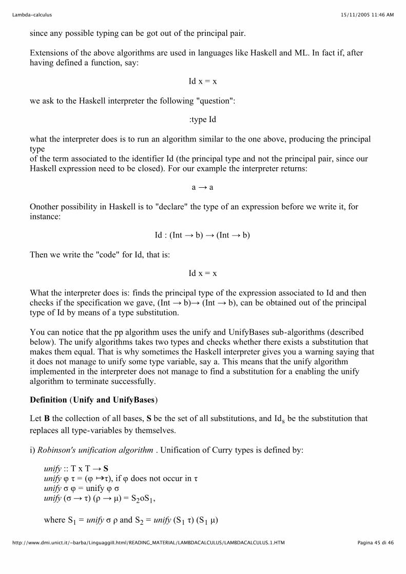
15/11/2005 11:46 AMLambda-calculus
Pagina 45 di 46http://www.dmi.unict.it/~barba/LinguaggiII.html/READING_MATERIAL/LAMBDACALCULUS/LAMBDACALCULUS.1.HTM
since any possible typing can be got out of the principal pair.
Extensions of the above algorithms are used in languages like Haskell and ML. In fact if, afterhaving defined a function, say:
Id x = x
we ask to the Haskell interpreter the following "question":
:type Id
what the interpreter does is to run an algorithm similar to the one above, producing the principaltypeof the term associated to the identifier Id (the principal type and not the principal pair, since ourHaskell expression need to be closed). For our example the interpreter returns:
a → a
Onother possibility in Haskell is to "declare" the type of an expression before we write it, forinstance:
Id : (Int → b) → (Int → b)
Then we write the "code" for Id, that is:
Id x = x
What the interpreter does is: finds the principal type of the expression associated to Id and thenchecks if the specification we gave, (Int → b)→ (Int → b), can be obtained out of the principaltype of Id by means of a type substitution.
You can notice that the pp algorithm uses the unify and UnifyBases sub-algorithms (describedbelow). The unify algorithms takes two types and checks whether there exists a substitution thatmakes them equal. That is why sometimes the Haskell interpreter gives you a warning saying thatit does not manage to unify some type variable, say a. This means that the unify algorithmimplemented in the interpreter does not manage to find a substitution for a enabling the unifyalgorithm to terminate successfully.
Definition (Unify and UnifyBases)
Let B the collection of all bases, S be the set of all substitutions, and Ids be the substitution thatreplaces all type-variables by themselves.
i) Robinson's unification algorithm . Unification of Curry types is defined by:
unify :: T x T → S unify φ τ = (φ τ), if φ does not occur in τ unify σ φ = unify φ σ unify (σ → τ) (ρ → µ) = S2oS1,
where S1 = unify σ ρ and S2 = unify (S1 τ) (S1 µ)
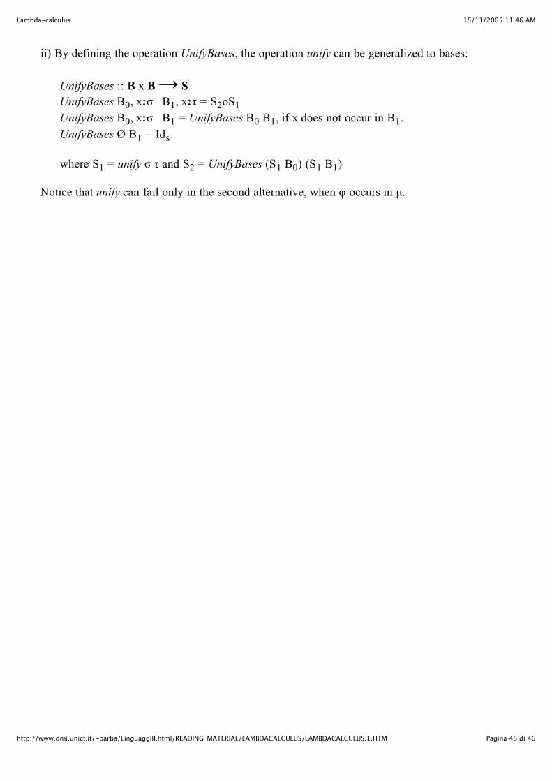
15/11/2005 11:46 AMLambda-calculus
Pagina 46 di 46http://www.dmi.unict.it/~barba/LinguaggiII.html/READING_MATERIAL/LAMBDACALCULUS/LAMBDACALCULUS.1.HTM
ii) By defining the operation UnifyBases, the operation unify can be generalized to bases:
UnifyBases :: B x B → S UnifyBases B0, x:σ B1, x:τ = S2oS1 UnifyBases B0, x:σ B1 = UnifyBases B0 B1, if x does not occur in B1. UnifyBases Ø B1 = Ids.
where S1 = unify σ τ and S2 = UnifyBases (S1 B0) (S1 B1)
Notice that unify can fail only in the second alternative, when φ occurs in µ.


![Lambda Calculus - SJTUyuxi/teaching/lectures/Lambda Calculus.pdf · Lambda Calculus Alonzo Church [14Jun.1903-11Aug.1995] invented the -Calculus with a foundational motivation [1932].](https://static.fdocument.org/doc/165x107/5fb2b5193e095c5efe6ac4f7/lambda-calculus-sjtu-yuxiteachinglectureslambda-calculuspdf-lambda-calculus.jpg)
![COMP4630: [fg]structure-Calculus - 1. BasicsIntroduction Lambda Calculus Terms Alpha Equivalence Substitution Dynamics Beta Reduction Eta Reduction Normal Forms Evaluation Strategies](https://static.fdocument.org/doc/165x107/5fd846ab2233da093f0d9793/comp4630-fgstructure-calculus-1-basics-introduction-lambda-calculus-terms.jpg)