Short Course_Macro-mechanics of Lamina
80
© 2003, P. Joyce
description
Macro Mechanix
Transcript of Short Course_Macro-mechanics of Lamina

© 2003, P. Joyce
MacromechanicalMacromechanical Analysis of a Analysis of a LaminaLamina
© 2003, P. Joyce
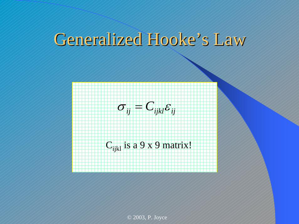
Generalized Generalized Hooke’s Hooke’s LawLaw
ijijklij C εσ =
Cijkl is a 9 x 9 matrix!
© 2003, P. Joyce
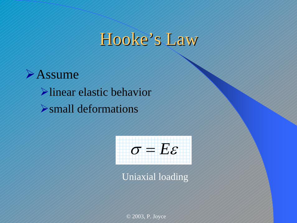
Hooke’sHooke’s LawLaw
Assume linear elastic behaviorsmall deformations
εσ E=
Uniaxial loading
© 2003, P. Joyce
TriaxialTriaxial Stress StateStress State
Shears are omittedConsider shear separatelySuperimpose three uniaxialstresses
x
z
y
x
z
y Uniaxial: σxUniaxial: σx
σx
x
z
y
σx
xxδ
dxE
dx xxxx
σ=ε=δ
Uniaxial: σx
σx
x
z
y
σx
yxδdy
Edy x
xyxσ
υ−=υε−=δ
dxE
dx xxxx
σ=ε=δ
Uniaxial: σx
σx
x
z
y
σx
zxδ
dxE
dx xxxx
σ=ε=δ
dyE
dy xxyx
συ−=υε−=δ
dzE
dz xxzx
συ−=υε−=δ
x
z
y Uniaxial: σyUniaxial: σy
σy
σx
x
z
y σy
dyE
dy yyyy
σ=ε=δ
yyδ
Uniaxial: σy
σy
σx
x
z
y σy
xyδ
dyE
dy yyyy
σ=ε=δ
dxE
dx yyxy
συ−=υε−=δ
Uniaxial: σy
σy
σx
x
z
y σy
zyδ dyE
dy yyyy
σ=ε=δ
dyE
dy yyxy
συ−=υε−=δ
dzE
dz yyzy
συ−=υε−=δ
x
z
y Uniaxial: σzUniaxial: σz
dzE
dz zzzz
σ=ε=δ
σz
x
z
y
zzδσz
Uniaxial: σz
dxE
dx zzxz
συ−=υε−=δ
dzE
dz zzzz
σ=ε=δ
σz
x
z
y
xzδσz
Uniaxial: σz
dxE
dx zzxz
συ−=υε−=δ
dzE
dz zzzz
σ=ε=δ
σz
x
z
y
yzδ
σz
dyE
dy zzyz
συ−=υε−=δ
xzxyxxxx dx δ+δ+δ=ε=δ xzxyxxxx dx δ+δ+δ=ε=δ
dxE
dxE
dxE
dx zyxxx
συ−
συ−
σ=ε=δ
xzxyxxxx dx δ+δ+δ=ε=δ
EEEzyx
xσ
υ−σ
υ−σ
=ε
dxE
dxE
dxE
dx zyxxx
συ−
συ−
σ=ε=δ
xzxyxxxx dx δ+δ+δ=ε=δ
EEEzyx
xσ
υ−σ
υ−σ
=ε
dxE
dxE
dxE
dx zyxxx
συ−
συ−
σ=ε=δ
( )[ ]zyxx E1 σ+συ−σ=ε
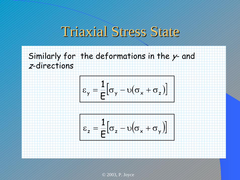
Similarly for the deformations in the y- and z-directions
( )[ ]yxzz E1 σ+συ−σ=ε
( )[ ]zxyy E1 σ+συ−σ=ε
© 2003, P. Joyce
Triaxial Triaxial Stress StateStress State
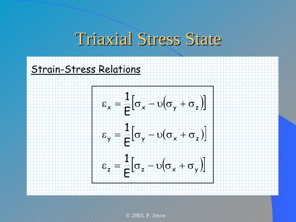
( )[ ]zyxx E1 σ+συ−σ=ε
( )[ ]yxzz E1 σ+συ−σ=ε
( )[ ]zxyy E1 σ+συ−σ=ε
Strain-Stress Relations
© 2003, P. Joyce
Triaxial Triaxial Stress StateStress State
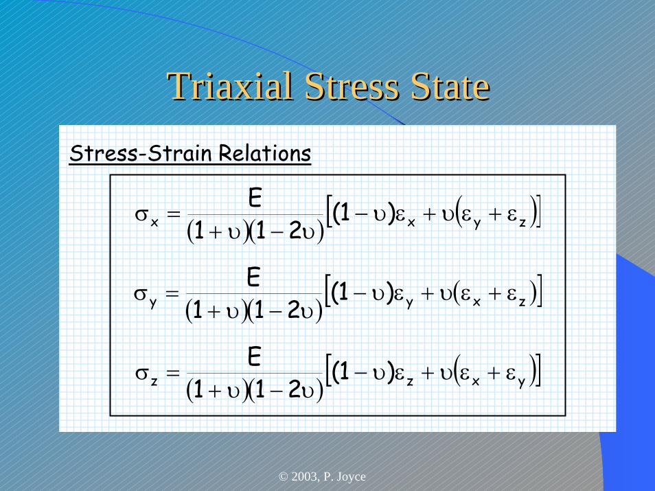
( )( )( )[ ]zyxx )1(
211E ε+ευ+ευ−
υ−υ+=σ
( )( )( )[ ]zxyy )1(
211E ε+ευ+ευ−
υ−υ+=σ
( )( )( )[ ]yxzz )1(
211E ε+ευ+ευ−
υ−υ+=σ
Stress-Strain Relations
© 2003, P. Joyce
Similarly for shear stressesSimilarly for shear stresses
© 2003, P. Joyce
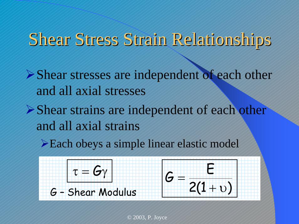
Shear Stress Strain RelationshipsShear Stress Strain Relationships
Shear stresses are independent of each other and all axial stressesShear strains are independent of each other and all axial strains
Each obeys a simple linear elastic model
G – Shear Modulus
γ=τ GG – Shear Modulus
γ=τ G)1(2
EGυ+
=

© 2003, P. Joyce
Shear StressShear Stress--Strain RelationshipsStrain Relationships
xyxyxy )1(2EG γ
υ+=γ=τ
xzxzxz )1(2EG γ
υ+=γ=τ
yzyzyz )1(2EG γ
υ+=γ=τ
© 2003, P. Joyce
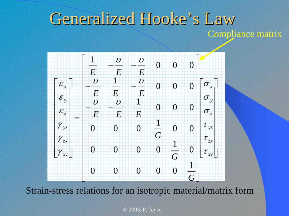
Generalized Generalized Hooke’s Hooke’s LawLaw
Strain-stress relations for an isotropic material/matrix form
⎥⎥⎥⎥⎥⎥⎥⎥
⎦
⎤
⎢⎢⎢⎢⎢⎢⎢⎢
⎣
⎡
⎥⎥⎥⎥⎥⎥⎥⎥⎥⎥⎥⎥⎥
⎦
⎤
⎢⎢⎢⎢⎢⎢⎢⎢⎢⎢⎢⎢⎢
⎣
⎡
−−
−−
−−
=
⎥⎥⎥⎥⎥⎥⎥⎥
⎦
⎤
⎢⎢⎢⎢⎢⎢⎢⎢
⎣
⎡
xy
zx
yz
z
y
x
xy
zx
yz
z
y
x
G
G
G
EEE
EEE
EEE
τττσσσ
υυ
υυ
υυ
γγγεεε
100000
010000
001000
0001
0001
0001
Compliance matrix
© 2003, P. Joyce
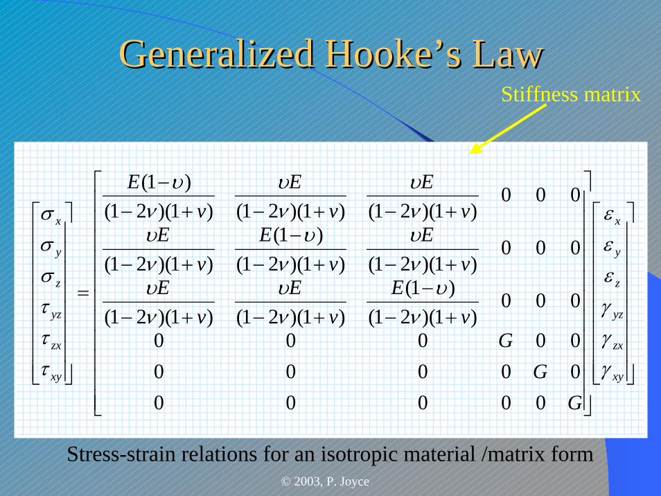
Generalized Generalized Hooke’s Hooke’s LawLaw
Stress-strain relations for an isotropic material /matrix form
⎥⎥⎥⎥⎥⎥⎥⎥
⎦
⎤
⎢⎢⎢⎢⎢⎢⎢⎢
⎣
⎡
⎥⎥⎥⎥⎥⎥⎥⎥⎥⎥⎥
⎦
⎤
⎢⎢⎢⎢⎢⎢⎢⎢⎢⎢⎢
⎣
⎡
+−−
+−+−
+−+−−
+−
+−+−+−−
=
⎥⎥⎥⎥⎥⎥⎥⎥
⎦
⎤
⎢⎢⎢⎢⎢⎢⎢⎢
⎣
⎡
xy
zx
yz
z
y
x
xy
zx
yz
z
y
x
GG
Gv
Ev
Ev
Ev
Ev
Ev
Ev
Ev
Ev
E
γγγεεε
νυ
νυ
νυ
νυ
νυ
νυ
νυ
νυ
νυ
τττσσσ
000000000000000
000)1)(21(
)1()1)(21()1)(21(
000)1)(21()1)(21(
)1()1)(21(
000)1)(21()1)(21()1)(21(
)1(
Stiffness matrix
© 2003, P. Joyce
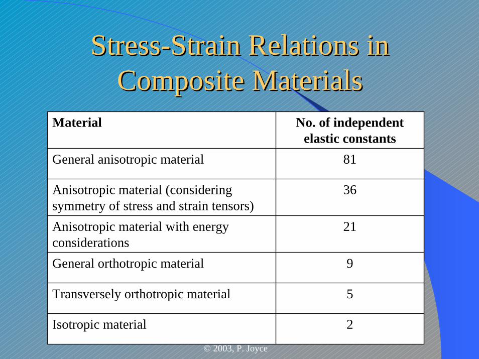
StressStress--Strain Relations in Strain Relations in Composite MaterialsComposite Materials
Material No. of independent elastic constants
General anisotropic material 81
Anisotropic material (considering symmetry of stress and strain tensors)
36
Anisotropic material with energy considerations
21
General orthotropic material 9
Transversely orthotropic material 5
Isotropic material 2
© 2003, P. Joyce
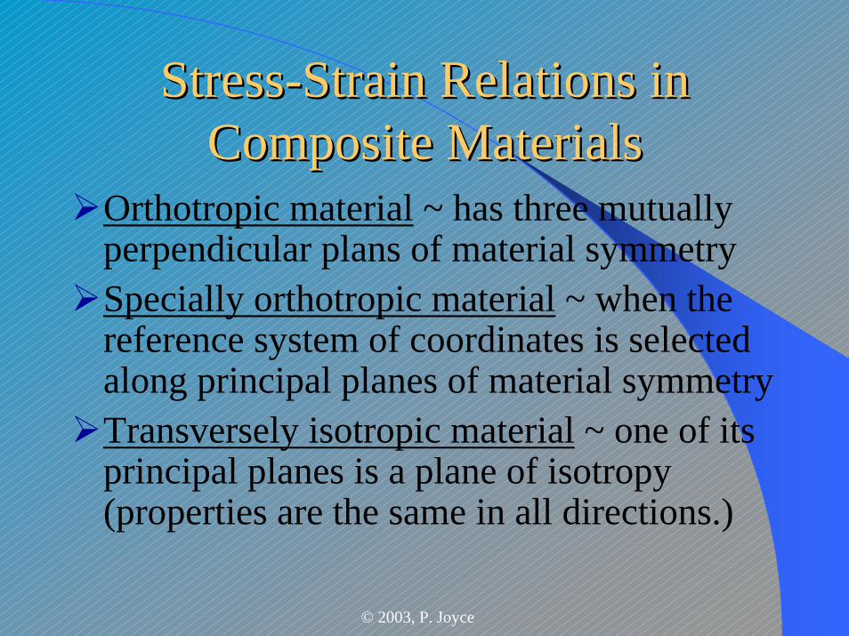
StressStress--Strain Relations in Strain Relations in Composite MaterialsComposite Materials
Orthotropic material ~ has three mutually perpendicular plans of material symmetrySpecially orthotropic material ~ when the reference system of coordinates is selected along principal planes of material symmetryTransversely isotropic material ~ one of its principal planes is a plane of isotropy (properties are the same in all directions.)
© 2003, P. Joyce
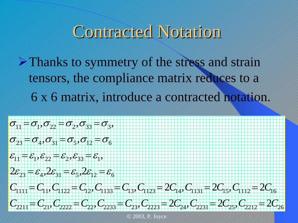
Contracted NotationContracted NotationThanks to symmetry of the stress and strain tensors, the compliance matrix reduces to a6 x 6 matrix, introduce a contracted notation.
262212252231242223232233222222212211
161112151131141123131133121122111111
612531423
133222111
612531423
333222111
2,2,2,,,2,2,2,,,
2,2,2,,,
,,,,,
CCCCCCCCCCCCCCCCCCCCCCCC
============
======
======
εεεεεεεεεεεε
σσσσσσσσσσσσ
© 2003, P. Joyce
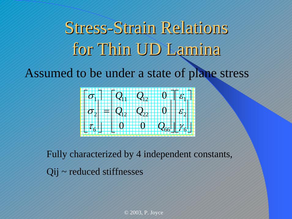
StressStress--Strain RelationsStrain Relationsfor Thin UD Laminafor Thin UD Lamina
Assumed to be under a state of plane stress
⎥⎥⎥
⎦
⎤
⎢⎢⎢
⎣
⎡
⎥⎥⎥
⎦
⎤
⎢⎢⎢
⎣
⎡=
⎥⎥⎥
⎦
⎤
⎢⎢⎢
⎣
⎡
6
2
1
66
2212
1211
6
2
1
0000
γεε
τσσ
QQQQQ
Fully characterized by 4 independent constants,
Qij ~ reduced stiffnesses
© 2003, P. Joyce
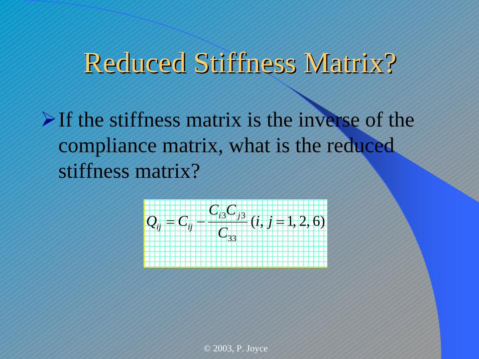
Reduced Stiffness Matrix?Reduced Stiffness Matrix?
If the stiffness matrix is the inverse of the compliance matrix, what is the reduced stiffness matrix?
)6 ,2 ,1,( 33
33 =−= jiC
CCCQ ji
ijij
© 2003, P. Joyce
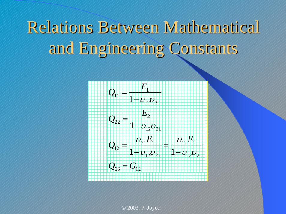
Relations Between Mathematical Relations Between Mathematical and Engineering Constantsand Engineering Constants
1266
2112
212
2112
12112
2112
222
2112
111
11
1
1
GQ
EEQ
EQ
EQ
=−
=−
=
−=
−=
υυυ
υυυ
υυ
υυ
© 2003, P. Joyce
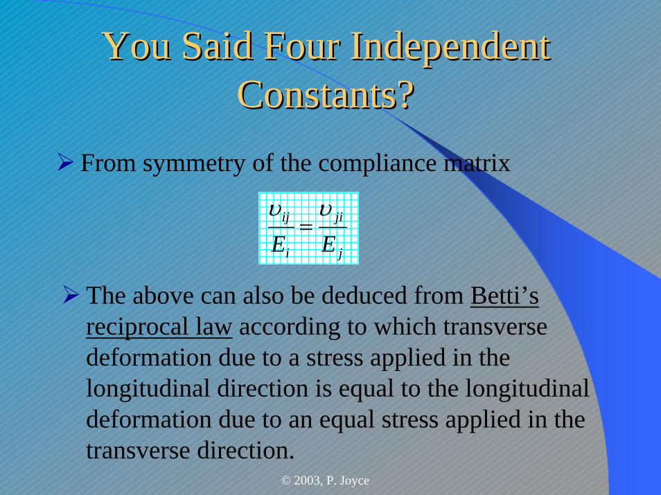
You Said Four Independent You Said Four Independent Constants?Constants?
From symmetry of the compliance matrix
j
ji
i
ij
EEυυ
=
The above can also be deduced from Betti’s reciprocal law according to which transverse deformation due to a stress applied in the longitudinal direction is equal to the longitudinal deformation due to an equal stress applied in the transverse direction.
© 2003, P. Joyce
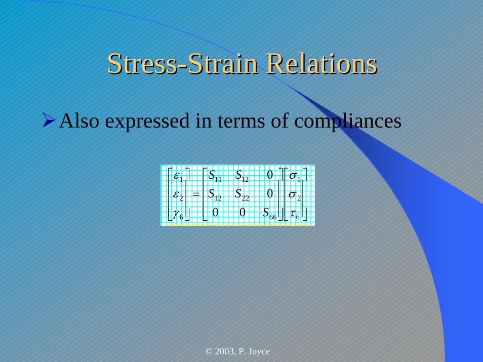
StressStress--Strain RelationsStrain Relations
Also expressed in terms of compliances
⎥⎥⎥
⎦
⎤
⎢⎢⎢
⎣
⎡
⎥⎥⎥
⎦
⎤
⎢⎢⎢
⎣
⎡=
⎥⎥⎥
⎦
⎤
⎢⎢⎢
⎣
⎡
6
2
1
66
2212
1211
6
2
1
0000
τσσ
γεε
SSSSS
© 2003, P. Joyce
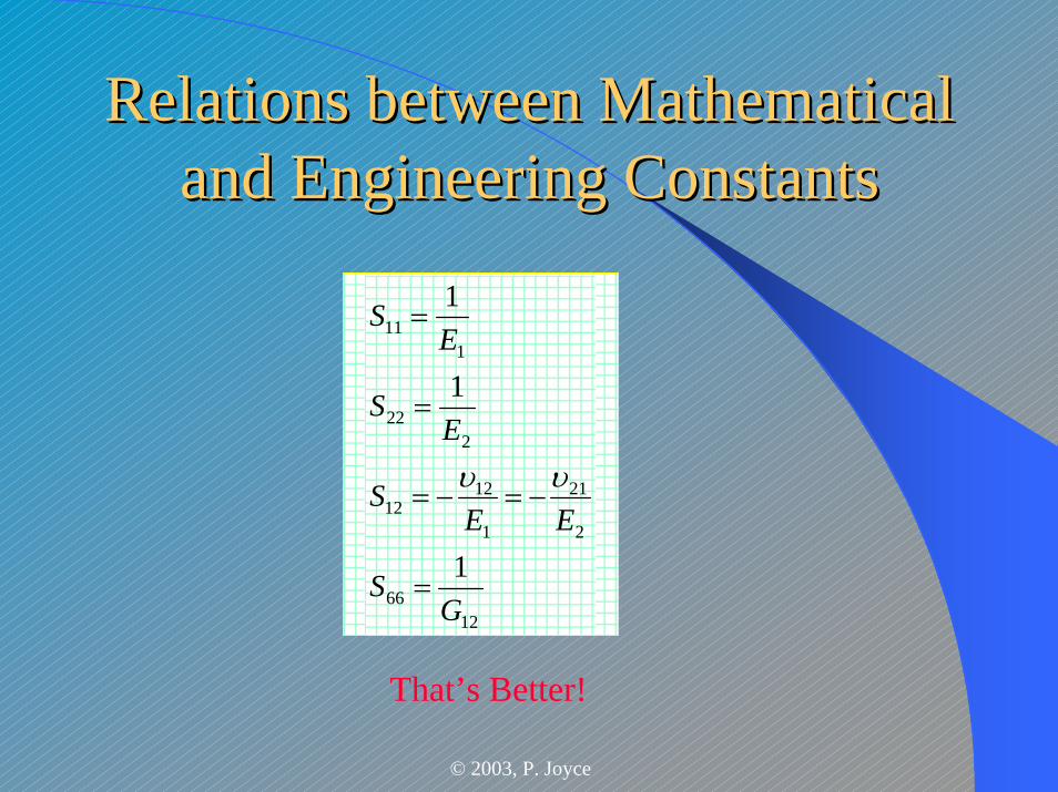
Relations between Mathematical Relations between Mathematical and Engineering Constantsand Engineering Constants
1266
2
21
1
1212
222
111
1
1
1
GS
EES
ES
ES
=
−=−=
=
=
υυ
That’s Better!
© 2003, P. Joyce
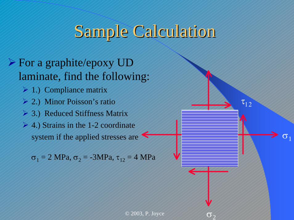
Sample CalculationSample CalculationFor a graphite/epoxy UD laminate, find the following:
1.) Compliance matrix2.) Minor Poisson’s ratio3.) Reduced Stiffness Matrix4.) Strains in the 1-2 coordinate system if the applied stresses are
σ1 = 2 MPa, σ2 = -3MPa, τ12 = 4 MPa
σ1
σ2
τ12
© 2003, P. Joyce
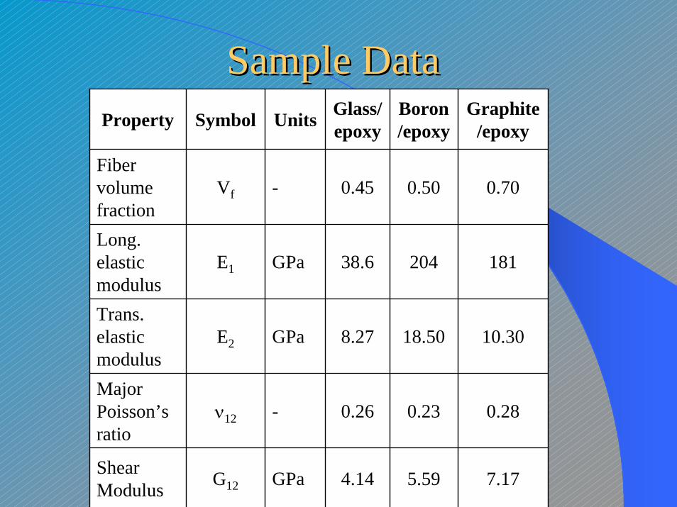
Sample DataSample DataProperty Symbol Units Glass/
epoxyBoron/epoxy
Graphite/epoxy
Fiber volume fraction
Vf - 0.45 0.50 0.70
Long. elastic modulus
E1 GPa 38.6 204 181
Trans. elastic modulus
E2 GPa 8.27 18.50 10.30
Major Poisson’s ratio
ν12 - 0.26 0.23 0.28
Shear Modulus G12 GPa 4.14 5.59 7.17
© 2003, P. Joyce
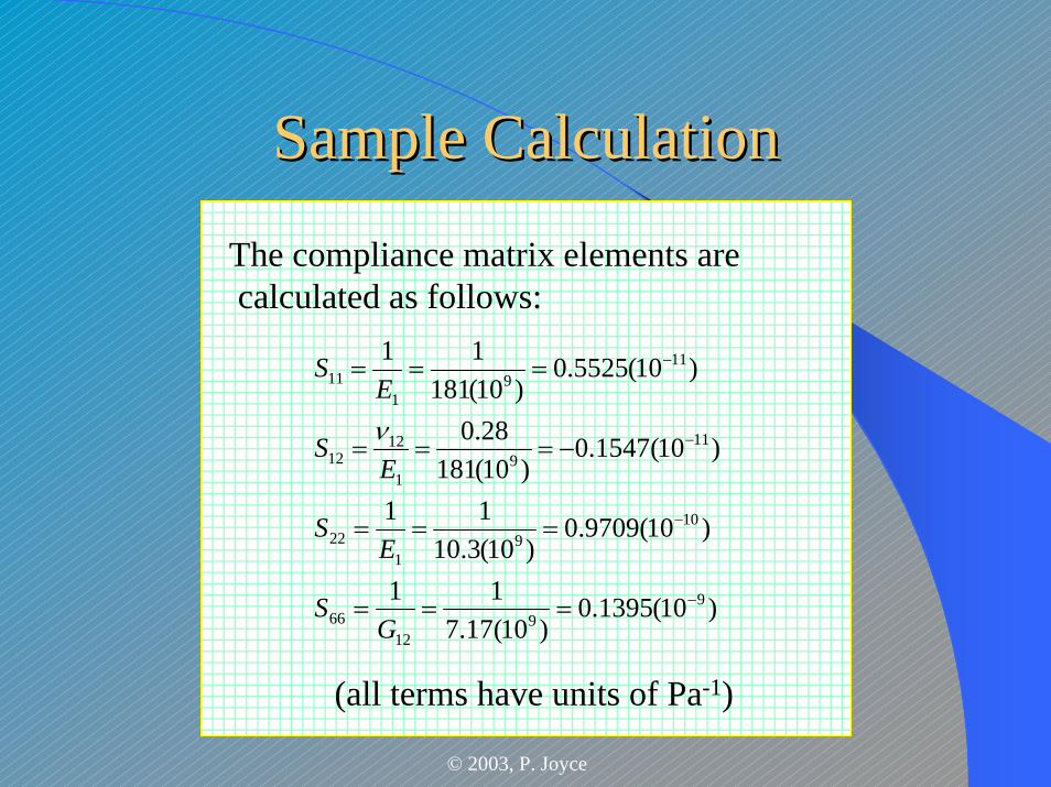
Sample CalculationSample Calculation
)10(1395.0)10(17.7
11
)10(9709.0)10(3.10
11
)10(1547.0)10(181
28.0
)10(5525.0)10(181
11
99
1266
109
122
119
1
1212
119
111
−
−
−
−
===
===
−===
===
GS
ES
ES
ES
ν
The compliance matrix elements arecalculated as follows:
(all terms have units of Pa-1)

© 2003, P. Joyce
Sample CalculationSample Calculation
01593.0)10)(3.10()10(181
)28.0( 9921
1
12
2
21
==
=
ν
ννEE
From Betti’s reciprocal law:
© 2003, P. Joyce
Sample CalculationSample Calculation
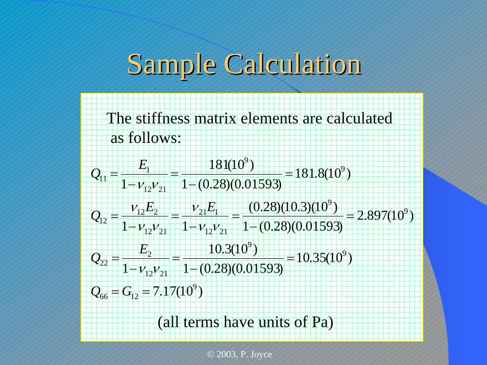
)10(17.7
)10(35.10)01593.0)(28.0(1
)10(3.101
)10(897.2)01593.0)(28.0(1
)10)(3.10)(28.0(11
)10(8.181)01593.0)(28.0(1
)10(1811
91266
99
2112
222
99
2112
121
2112
21212
99
2112
111
==
=−
=−
=
=−
=−
=−
=
=−
=−
=
GQ
EQ
EEQ
EQ
νν
ννν
ννν
νν
The stiffness matrix elements are calculatedas follows:
(all terms have units of Pa)
© 2003, P. Joyce
Sample CalculationSample Calculation
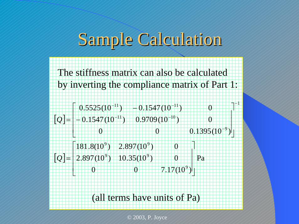
[ ]
[ ] Pa )10(17.700
0)10(35.10)10(897.20)10(897.2)10(8.181
)10(1395.0000)10(9709.0)10(1547.00)10(1547.0)10(5525.0
9
99
99
1
9
1011
1111
⎥⎥⎥
⎦
⎤
⎢⎢⎢
⎣
⎡
=
⎥⎥⎥
⎦
⎤
⎢⎢⎢
⎣
⎡
−−
=
−
−
−−
−−
Q
Q
The stiffness matrix can also be calculatedby inverting the compliance matrix of Part 1:
(all terms have units of Pa)
© 2003, P. Joyce
Sample CalculationSample Calculation
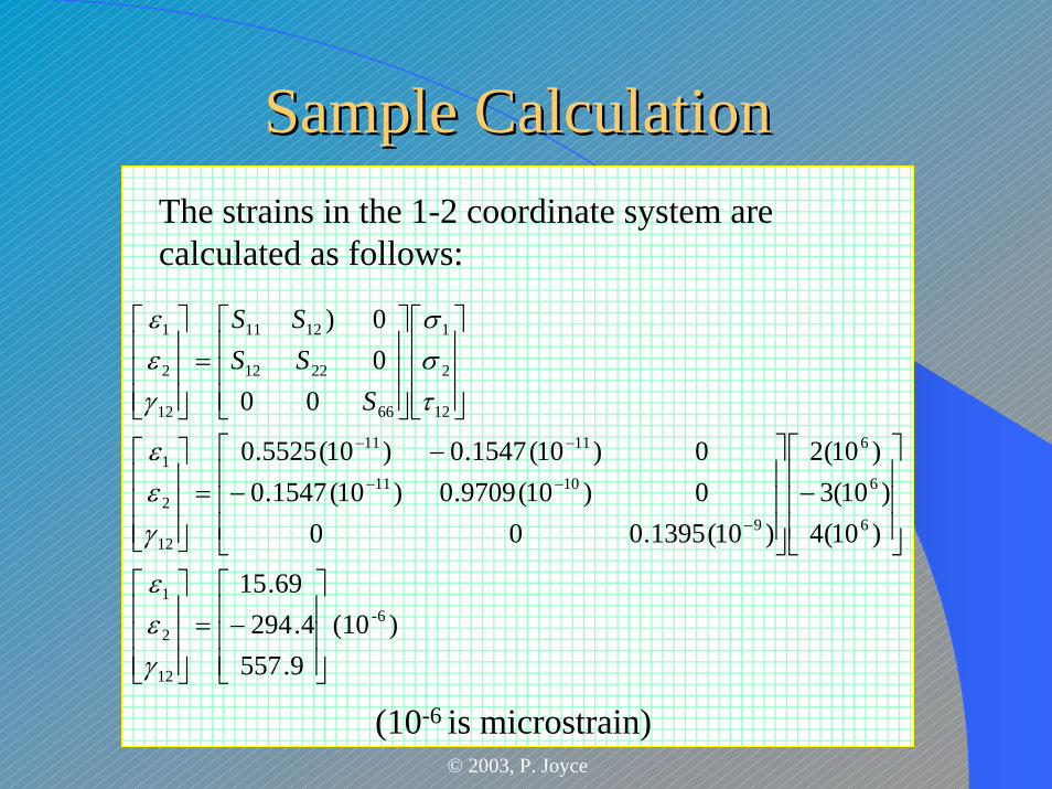
)(10 9.5574.294
69.15
)10(4)10(3
)10(2
)10(1395.0000)10(9709.0)10(1547.00)10(1547.0)10(5525.0
0000)
6-
12
2
1
6
6
6
9
1011
1111
12
2
1
12
2
1
66
2212
1211
12
2
1
⎥⎥⎥
⎦
⎤
⎢⎢⎢
⎣
⎡−=
⎥⎥⎥
⎦
⎤
⎢⎢⎢
⎣
⎡
⎥⎥⎥
⎦
⎤
⎢⎢⎢
⎣
⎡
−⎥⎥⎥
⎦
⎤
⎢⎢⎢
⎣
⎡
−−
=⎥⎥⎥
⎦
⎤
⎢⎢⎢
⎣
⎡
⎥⎥⎥
⎦
⎤
⎢⎢⎢
⎣
⎡
⎥⎥⎥
⎦
⎤
⎢⎢⎢
⎣
⎡=
⎥⎥⎥
⎦
⎤
⎢⎢⎢
⎣
⎡
−
−−
−−
γεε
γεε
τσσ
γεε
SSSSS
The strains in the 1-2 coordinate system arecalculated as follows:
(10-6 is microstrain)
© 2003, P. Joyce
StressStress--Strain RelationsStrain Relationsfor Thin Angle Laminafor Thin Angle Lamina
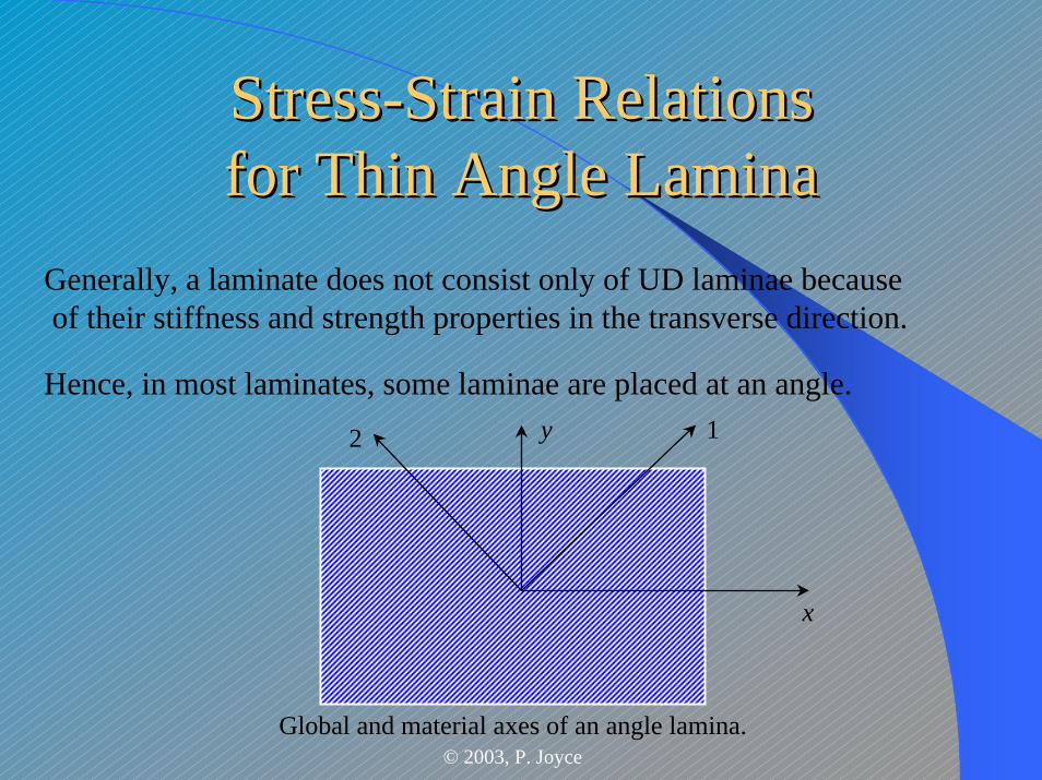
Generally, a laminate does not consist only of UD laminae becauseof their stiffness and strength properties in the transverse direction.
Hence, in most laminates, some laminae are placed at an angle.
x
y 12
Global and material axes of an angle lamina.
© 2003, P. Joyce
StressStress--Strain RelationsStrain Relationsfor Thin Angle Laminafor Thin Angle Lamina
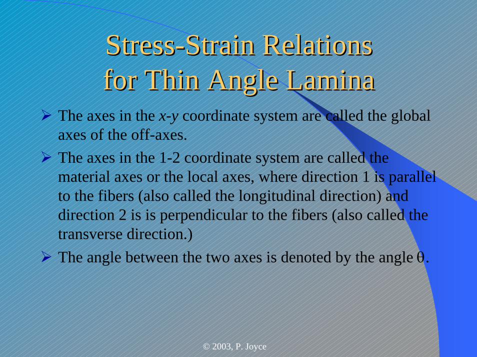
The axes in the x-y coordinate system are called the global axes of the off-axes.The axes in the 1-2 coordinate system are called the material axes or the local axes, where direction 1 is parallel to the fibers (also called the longitudinal direction) and direction 2 is is perpendicular to the fibers (also called the transverse direction.)The angle between the two axes is denoted by the angle θ.
© 2003, P. Joyce
StressStress--Strain RelationsStrain Relationsfor Thin Angle Laminafor Thin Angle Lamina
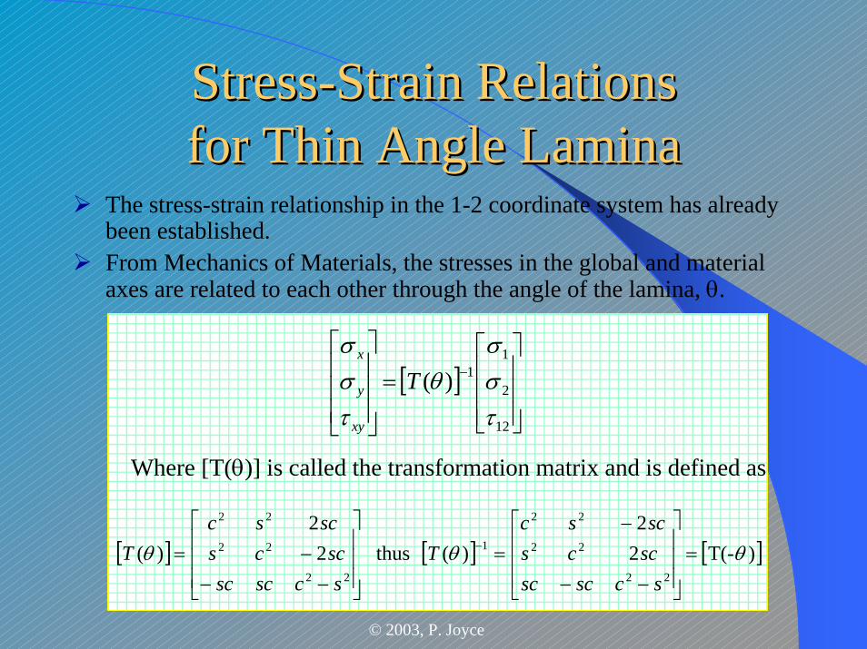
The stress-strain relationship in the 1-2 coordinate system has already been established.From Mechanics of Materials, the stresses in the global and material axes are related to each other through the angle of the lamina, θ.
[ ]⎥⎥⎥
⎦
⎤
⎢⎢⎢
⎣
⎡=
⎥⎥⎥
⎦
⎤
⎢⎢⎢
⎣
⎡−
12
2
11)(
τσσ
θτσσ
T
xy
y
x
Where [T(θ)] is called the transformation matrix and is defined as
[ ] [ ] [ ])T(- 22
)( thus22
)(22
22
22
1
22
22
22
θθθ =⎥⎥⎥
⎦
⎤
⎢⎢⎢
⎣
⎡
−−
−=
⎥⎥⎥
⎦
⎤
⎢⎢⎢
⎣
⎡
−−−= −
scscscsccsscsc
Tscscsc
sccsscsc
T
© 2003, P. Joyce
StressStress--Strain RelationsStrain Relationsfor Thin Angle Laminafor Thin Angle Lamina
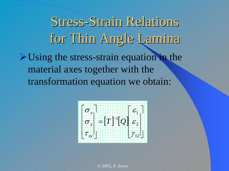
Using the stress-strain equation in the material axes together with the transformation equation we obtain:
[ ] [ ]⎥⎥⎥
⎦
⎤
⎢⎢⎢
⎣
⎡=
⎥⎥⎥
⎦
⎤
⎢⎢⎢
⎣
⎡−
12
2
11
γεε
τσσ
QT
xy
y
x
© 2003, P. Joyce
StressStress--Strain RelationsStrain Relationsfor Thin Angle Laminafor Thin Angle Lamina
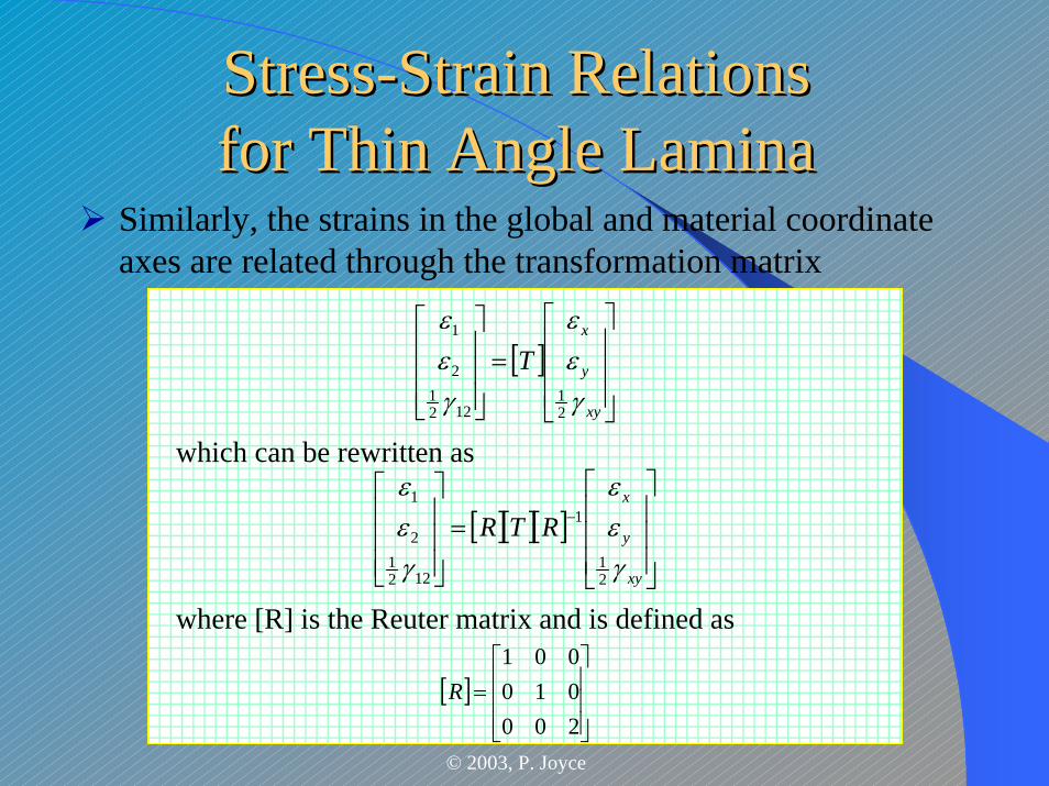
Similarly, the strains in the global and material coordinate axes are related through the transformation matrix
[ ]⎥⎥⎥
⎦
⎤
⎢⎢⎢
⎣
⎡
=⎥⎥⎥
⎦
⎤
⎢⎢⎢
⎣
⎡
xy
y
x
Tγεε
γεε
21
1221
2
1
which can be rewritten as
[ ][ ][ ]⎥⎥⎥
⎦
⎤
⎢⎢⎢
⎣
⎡
=⎥⎥⎥
⎦
⎤
⎢⎢⎢
⎣
⎡−
xy
y
x
RTRγεε
γεε
21
1
1221
2
1
where [R] is the Reuter matrix and is defined as
[ ]⎥⎥⎥
⎦
⎤
⎢⎢⎢
⎣
⎡=
200010001
R
© 2003, P. Joyce
StressStress--Strain RelationsStrain Relationsfor Thin Angle Laminafor Thin Angle Lamina
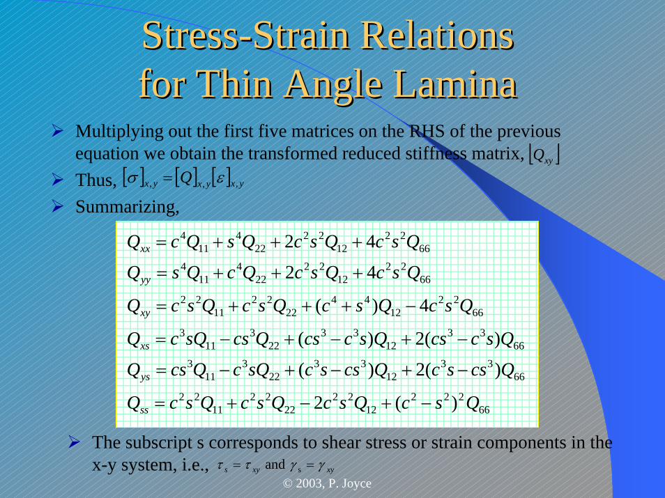
Multiplying out the first five matrices on the RHS of the previous equation we obtain the transformed reduced stiffness matrix, Thus, Summarizing,
66222
1222
2222
1122
6633
1233
223
113
6633
1233
223
113
6622
1244
2222
1122
6622
1222
224
114
6622
1222
224
114
)(2
)(2)(
)(2)(
4)(
42
42
QscQscQscQscQ
QcsscQcsscsQcQcsQ
QsccsQsccsQcssQcQ
QscQscQscQscQ
QscQscQcQsQ
QscQscQsQcQ
ss
ys
xs
xy
yy
xx
−+−+=
−+−+−=
−+−+−=
−+++=
+++=
+++=
[ ]xyQ[ ] [ ] [ ] yxyxyx Q ,,, εσ =
The subscript s corresponds to shear stress or strain components in the x-y system, i.e., xyxys γγττ == s and
© 2003, P. Joyce
StrainStrain--Stress Relations for Thin Stress Relations for Thin Angle LaminaAngle Lamina
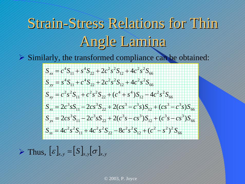
Similarly, the transformed compliance can be obtained:
66222
1222
2222
1122
6633
1233
223
113
6633
1233
223
113
6622
1244
2222
1122
6622
1222
224
114
6622
1222
224
114
)(844
)()(222
)()(222
4)(
42
42
SscSscSscSscS
ScsscScsscsScScsS
SsccsSsccsScssScS
SscSscSscSscS
SscSscScSsS
SscSscSsScS
ss
ys
xs
xy
yy
xx
−+−+=
−+−+−=
−+−+−=
−+++=
+++=
+++=
Thus, [ ] [ ] [ ] yxyxyx S ,,, σε =
© 2003, P. Joyce
StrainStrain--Stress Relations for Thin Stress Relations for Thin Angle LaminaAngle Lamina
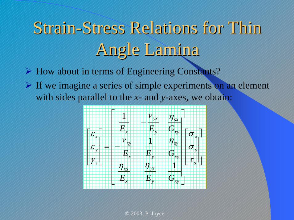
How about in terms of Engineering Constants?If we imagine a series of simple experiments on an element with sides parallel to the x- and y-axes, we obtain:
⎥⎥⎥
⎦
⎤
⎢⎢⎢
⎣
⎡
⎥⎥⎥⎥⎥⎥⎥
⎦
⎤
⎢⎢⎢⎢⎢⎢⎢
⎣
⎡
−
−
=⎥⎥⎥
⎦
⎤
⎢⎢⎢
⎣
⎡
s
y
x
xyy
ys
x
xs
xy
sy
yx
xy
xy
sx
y
yx
x
s
y
x
GEE
GEE
GEE
τσσ
ηη
ην
ην
γεε
1
1
1
© 2003, P. Joyce
StrainStrain--Stress Relations for Thin Stress Relations for Thin Angle LaminaAngle Lamina
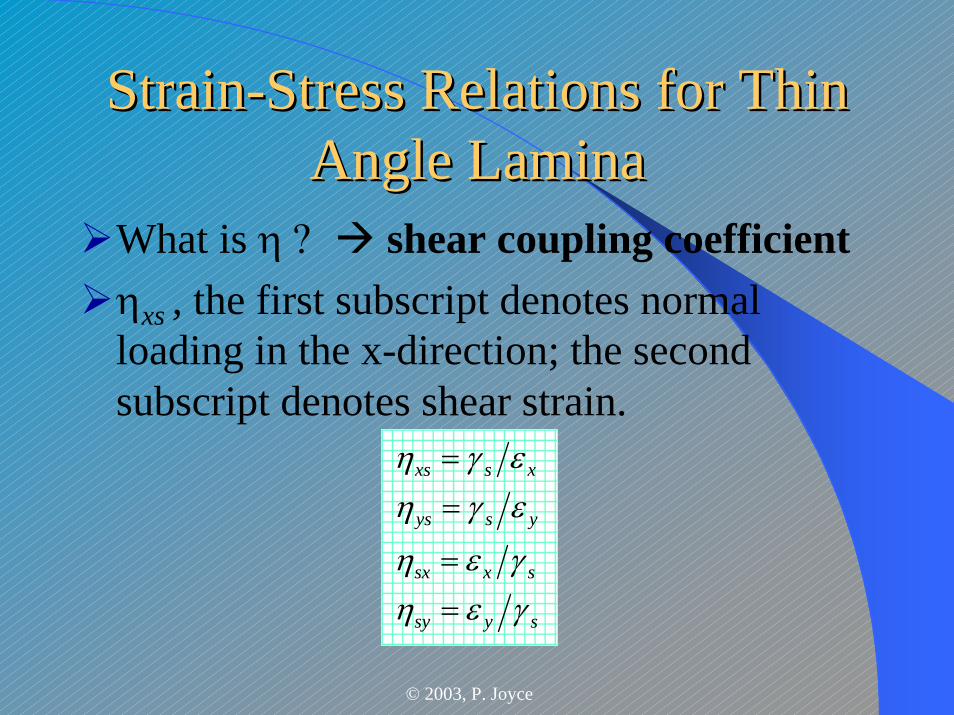
What is η ? shear coupling coefficientηxs , the first subscript denotes normal loading in the x-direction; the second subscript denotes shear strain.
sysy
sxsx
ysys
xsxs
γεηγεη
εγηεγη
==
==
© 2003, P. Joyce
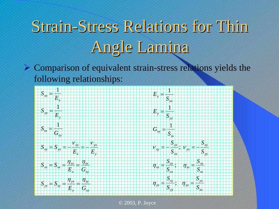
StrainStrain--Stress Relations for Thin Stress Relations for Thin Angle LaminaAngle Lamina
Comparison of equivalent strain-stress relations yields the following relationships:
xy
sy
y
yssyys
xy
sx
x
xssxxs
y
yx
x
xyyxxy
xyss
yyy
xxx
GESS
GESS
EESS
GS
ES
ES
ηη
ηη
νν
===
===
−=−==
=
=
=
1
1
1
ss
ysyx
yy
syys
ss
xssx
xx
sxxs
yy
xyyx
xx
yxxy
ssxy
yyy
xxx
SS
SS
SS
SS
SS
SS
SG
SE
SE
==
==
−=−=
=
=
=
ηη
ηη
νν
;
;
;
1
1
1
© 2003, P. Joyce
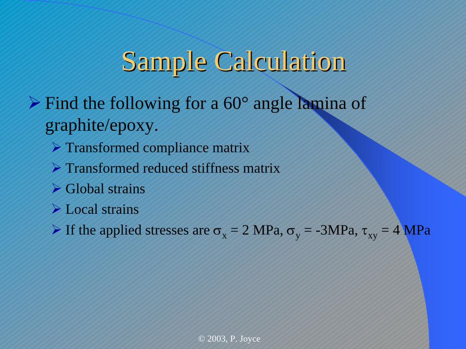
Sample CalculationSample CalculationFind the following for a 60° angle lamina of graphite/epoxy.
Transformed compliance matrixTransformed reduced stiffness matrixGlobal strainsLocal strainsIf the applied stresses are σx = 2 MPa, σy = -3MPa, τxy = 4 MPa
© 2003, P. Joyce
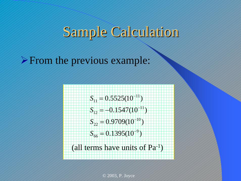
Sample CalculationSample Calculation
From the previous example:
)10(1395.0
)10(9709.0
)10(1547.0
)10(5525.0
966
1022
1112
1111
−
−
−
−
=
=
−=
=
S
S
S
S
(all terms have units of Pa-1)
© 2003, P. Joyce
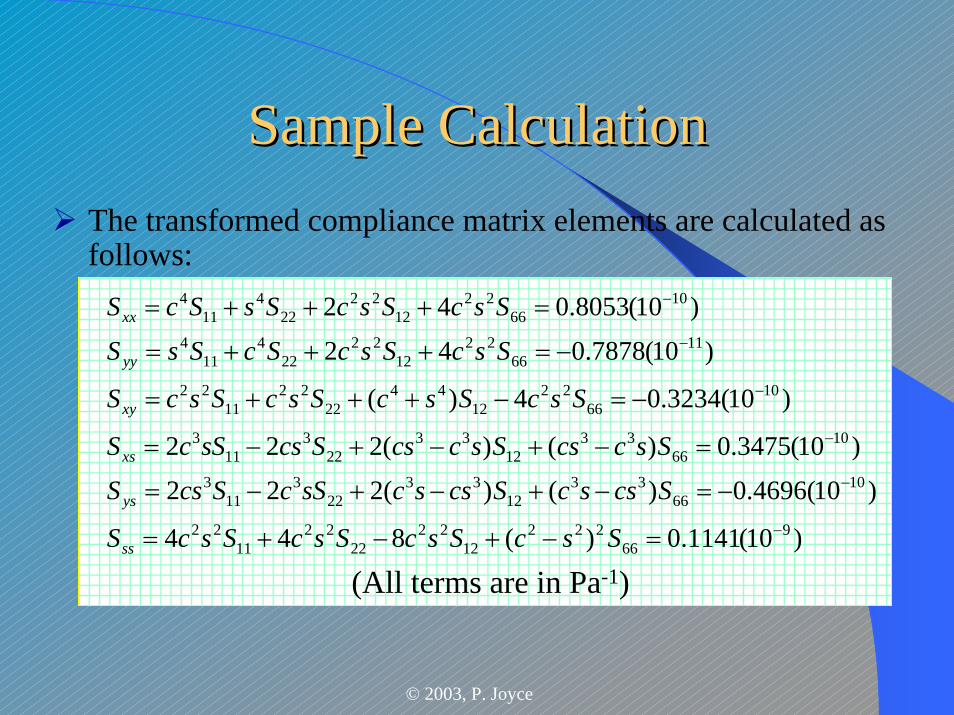
Sample CalculationSample CalculationThe transformed compliance matrix elements are calculated as follows:
)10(1141.0)(844
)10(4696.0)()(222
)10(3475.0)()(222
)10(3234.04)(
)10(7878.042
)10(8053.042
966
22212
2222
2211
22
1066
3312
3322
311
3
1066
3312
3322
311
3
1066
2212
4422
2211
22
1166
2212
2222
411
4
1066
2212
2222
411
4
−
−
−
−
−
−
=−+−+=
−=−+−+−=
=−+−+−=
−=−+++=
−=+++=
=+++=
SscSscSscSscS
ScsscScsscsScScsS
SsccsSsccsScssScS
SscSscSscSscS
SscSscScSsS
SscSscSsScS
ss
ys
xs
xy
yy
xx
(All terms are in Pa-1)
© 2003, P. Joyce
Sample CalculationSample Calculation
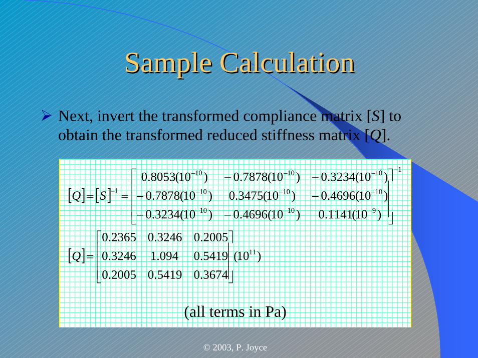
Next, invert the transformed compliance matrix [S] to obtain the transformed reduced stiffness matrix [Q].
[ ] [ ]
[ ] )10(3674.05419.02005.05419.0094.13246.02005.03246.02365.0
)10(1141.0)10(4696.0)10(3234.0)10(4696.0)10(3475.0)10(7878.0)10(3234.0)10(7878.0)10(8053.0
11
1
91010
101010
101010
1
⎥⎥⎥
⎦
⎤
⎢⎢⎢
⎣
⎡=
⎥⎥⎥
⎦
⎤
⎢⎢⎢
⎣
⎡
−−−−−−
==
−
−−−
−−−
−−−
−
Q
SQ
(all terms in Pa)
© 2003, P. Joyce
Sample CalculationSample Calculation
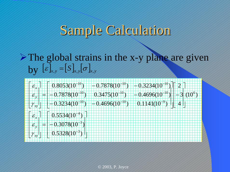
The global strains in the x-y plane are given by [ ] [ ] [ ] yxyxyx S ,,, σε =
⎥⎥⎥
⎦
⎤
⎢⎢⎢
⎣
⎡
−=⎥⎥⎥
⎦
⎤
⎢⎢⎢
⎣
⎡
⎥⎥⎥
⎦
⎤
⎢⎢⎢
⎣
⎡−
⎥⎥⎥
⎦
⎤
⎢⎢⎢
⎣
⎡
−−−−−−
=⎥⎥⎥
⎦
⎤
⎢⎢⎢
⎣
⎡
−
−
−
−−−
−−−
−−−
)10(5328.0)10(3078.0
)10(5534.0
)10(43
2
)10(1141.0)10(4696.0)10(3234.0)10(4696.0)10(3475.0)10(7878.0)10(3234.0)10(7878.0)10(8053.0
3
3
4
6
91010
101010
101010
xy
y
x
xy
y
x
γεε
γεε
© 2003, P. Joyce
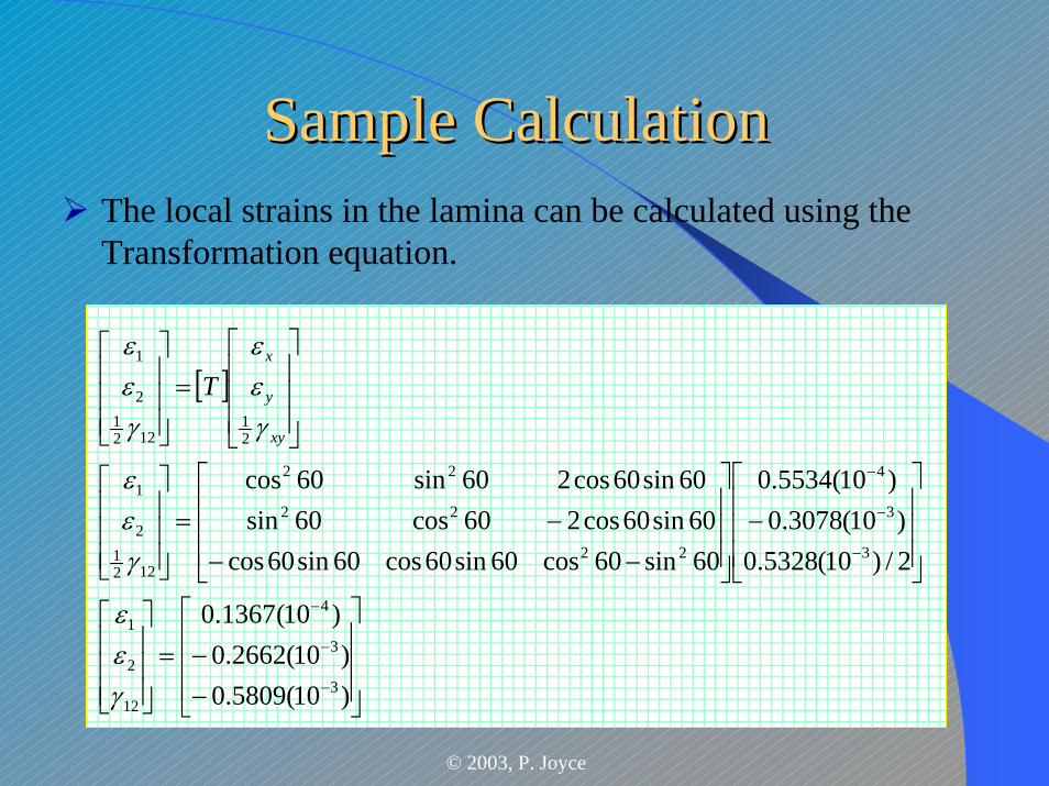
Sample CalculationSample CalculationThe local strains in the lamina can be calculated using the Transformation equation.
[ ]
⎥⎥⎥
⎦
⎤
⎢⎢⎢
⎣
⎡
−−=
⎥⎥⎥
⎦
⎤
⎢⎢⎢
⎣
⎡
⎥⎥⎥
⎦
⎤
⎢⎢⎢
⎣
⎡
−⎥⎥⎥
⎦
⎤
⎢⎢⎢
⎣
⎡
−−−=
⎥⎥⎥
⎦
⎤
⎢⎢⎢
⎣
⎡
⎥⎥⎥
⎦
⎤
⎢⎢⎢
⎣
⎡
=⎥⎥⎥
⎦
⎤
⎢⎢⎢
⎣
⎡
−
−
−
−
−
−
)10(5809.0)10(2662.0
)10(1367.0
2/)10(5328.0)10(3078.0
)10(5534.0
60sin60cos60sin60cos60sin60cos60sin60cos260cos60sin
60sin60cos260sin60cos
3
3
4
12
2
1
3
3
4
22
22
22
1221
2
1
21
1221
2
1
γεε
γεε
γεε
γεε
xy
y
x
T
© 2003, P. Joyce
Transformation ofTransformation ofEngineering ConstantsEngineering Constants
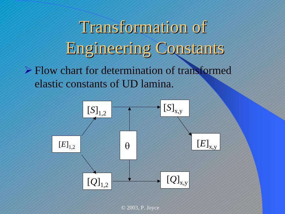
Flow chart for determination of transformed elastic constants of UD lamina.
[S]1,2
[E]1,2
[S]x,y
[Q]1,2[Q]x,y
θ [E]x,y
© 2003, P. Joyce
MacromechanicalMacromechanical Strength Strength ParametersParameters
From a macromechanical POV, the strength of a lamina is an anisotropic property.It is desirable, for example, to correlate the strength along an arbitrary direction to some basic strength parameters (analogous to micromechanic definitions before.)
© 2003, P. Joyce
Strength Failure Theories of an Strength Failure Theories of an Angle LaminaAngle Lamina
Various theories have been developed for studying the failure of an angle lamina.Generally based on the normal and shear strengths of a UD lamina.Need to consider tension and compressionUD lamina has 2 material axes, 1-direction parallel to the fibers and 2-direction which is perpendicular to the fibers.Hence there are 4 normal strength parameters for UD lamina.
Tensile strength in fiber directionTransverse tensile strengthCompressive strength in fiber directionTransverse compressive strength
The fifth strength parameter is the shear strength
© 2003, P. Joyce
Strength Failure Theories of an Strength Failure Theories of an Angle LaminaAngle Lamina
Unlike the stiffness parameters, these strength parameters cannot be transformed directly for an angle lamina.Hence, the failure theories are based on first finding the stresses in the material axes and then using these five strength parameters of a UD lamina to find whether the lamina has failed.
© 2003, P. Joyce
MacromechanicalMacromechanical Strength Strength ParametersParameters
Also predict transverse compressive strength and in-plane shear strength using micromechanics. . .Failure mechanisms vary greatly with material properties and type of loading.Even when predictions are accurate with regard to failure initiation at critical points, they are only approximate as far as global failure of the lamina is concerned.Furthermore, the possible interaction of failure mechanisms makes it difficult to obtain reliable strength predictions under a general type of loading.A macromechanical or phenomological approach to failure analysis may be preferable.
© 2003, P. Joyce
MacromechanicalMacromechanical Strength Strength ParametersParameters
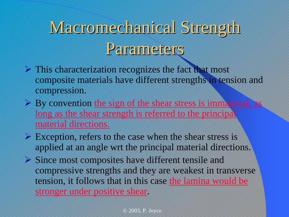
This characterization recognizes the fact that most composite materials have different strengths in tension and compression.By convention the sign of the shear stress is immaterial, as long as the shear strength is referred to the principal material directions.Exception, refers to the case when the shear stress is applied at an angle wrt the principal material directions.Since most composites have different tensile and compressive strengths and they are weakest in transverse tension, it follows that in this case the lamina would be stronger under positive shear.

© 2003, P. Joyce
MacromechanicalMacromechanical Strength Strength ParametersParametersτ6
σy = τ6
σx = -τ6Positive shear stress
Shear stress acting along principal material axes.
© 2003, P. Joyce
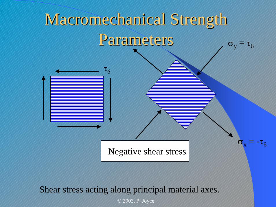
MacromechanicalMacromechanical Strength Strength ParametersParametersτ6
σy = τ6
σx = -τ6Negative shear stress
Shear stress acting along principal material axes.
© 2003, P. Joyce
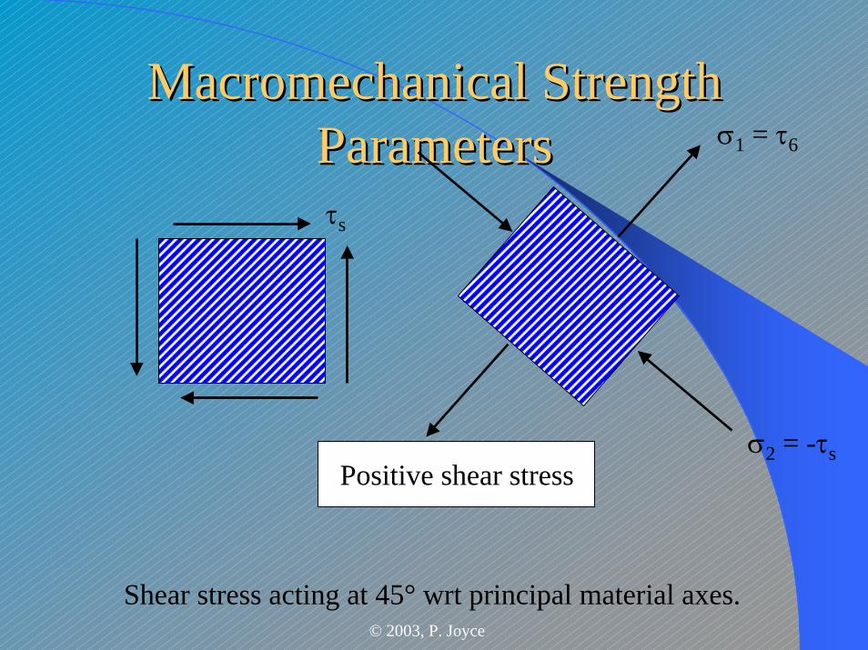
MacromechanicalMacromechanical Strength Strength ParametersParametersτs
σ1 = τ6
σ2 = -τsPositive shear stress
Shear stress acting at 45° wrt principal material axes.
© 2003, P. Joyce
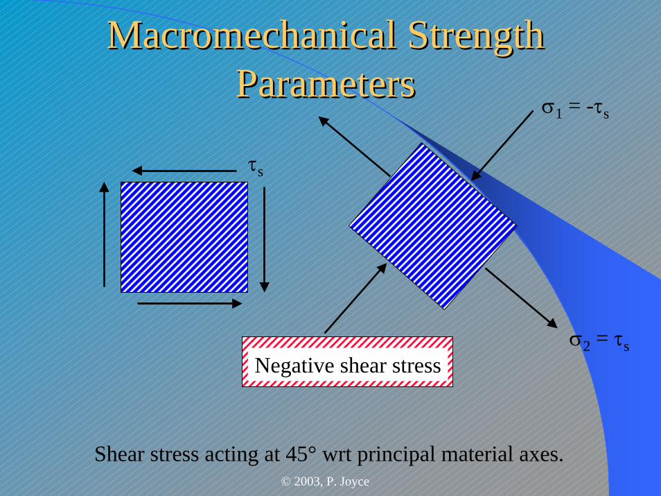
MacromechanicalMacromechanical Strength Strength ParametersParameters
τs
σ2 = τsNegative shear stress
σ1 = -τs
Shear stress acting at 45° wrt principal material axes.
© 2003, P. Joyce
MacromechanicalMacromechanical Failure Failure TheoriesTheories
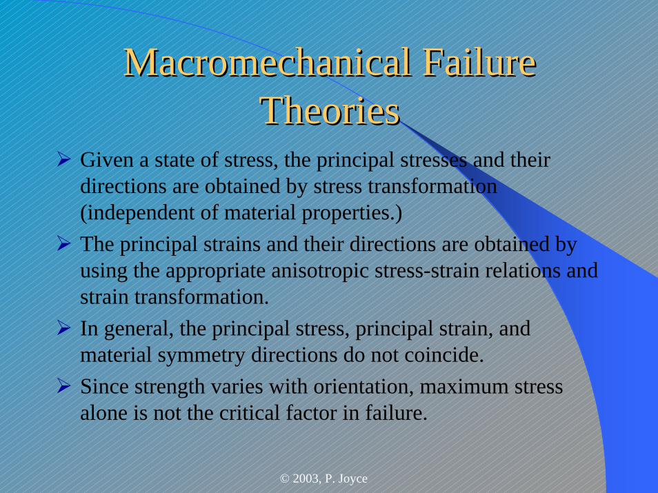
Given a state of stress, the principal stresses and their directions are obtained by stress transformation (independent of material properties.)The principal strains and their directions are obtained by using the appropriate anisotropic stress-strain relations and strain transformation.In general, the principal stress, principal strain, and material symmetry directions do not coincide.Since strength varies with orientation, maximum stress alone is not the critical factor in failure.
© 2003, P. Joyce
Macromechanical Macromechanical Failure Failure TheoriesTheories
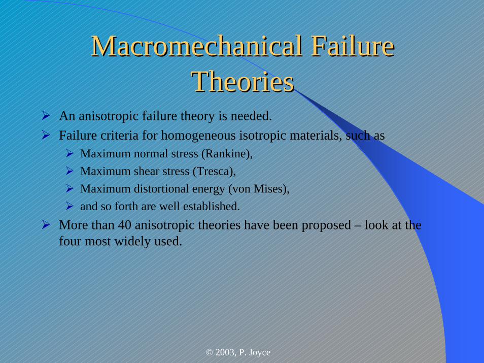
An anisotropic failure theory is needed.Failure criteria for homogeneous isotropic materials, such as
Maximum normal stress (Rankine), Maximum shear stress (Tresca), Maximum distortional energy (von Mises), and so forth are well established.
More than 40 anisotropic theories have been proposed – look at the four most widely used.
© 2003, P. Joyce
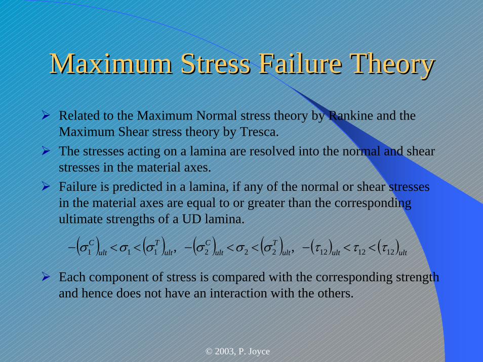
Maximum Stress Failure TheoryMaximum Stress Failure TheoryRelated to the Maximum Normal stress theory by Rankine and the Maximum Shear stress theory by Tresca.The stresses acting on a lamina are resolved into the normal and shear stresses in the material axes.Failure is predicted in a lamina, if any of the normal or shear stresses in the material axes are equal to or greater than the corresponding ultimate strengths of a UD lamina.
Each component of stress is compared with the corresponding strength and hence does not have an interaction with the others.
( ) ( ) ( ) ( ) ( ) ( )ultultultT
ultC
ultT
ultC
121212222111 , , τττσσσσσσ <<−<<−<<−
© 2003, P. Joyce
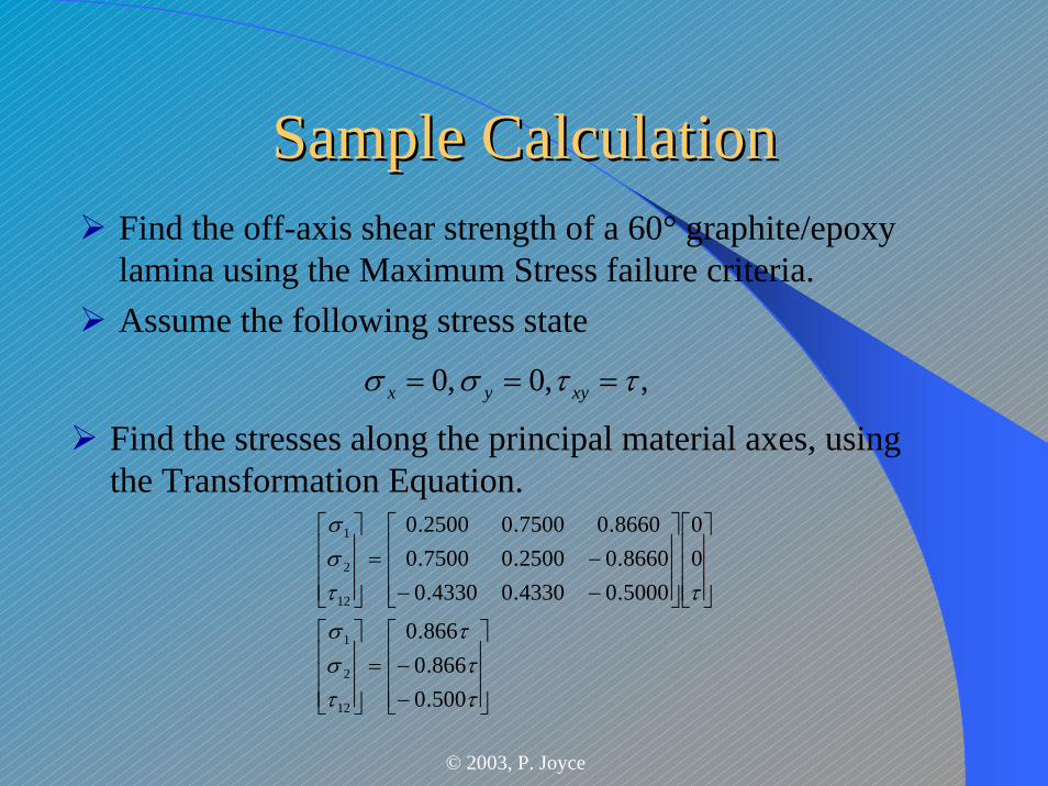
Sample CalculationSample CalculationFind the off-axis shear strength of a 60° graphite/epoxy lamina using the Maximum Stress failure criteria.Assume the following stress state
,,0 ,0 ττσσ === xyyx
Find the stresses along the principal material axes, using the Transformation Equation.
⎥⎥⎥
⎦
⎤
⎢⎢⎢
⎣
⎡
−−=
⎥⎥⎥
⎦
⎤
⎢⎢⎢
⎣
⎡
⎥⎥⎥
⎦
⎤
⎢⎢⎢
⎣
⎡
⎥⎥⎥
⎦
⎤
⎢⎢⎢
⎣
⎡
−−−=
⎥⎥⎥
⎦
⎤
⎢⎢⎢
⎣
⎡
ττ
τ
τσσ
ττσσ
500.0866.0
866.0
00
5000.04330.04330.08660.02500.07500.0
8660.07500.02500.0
12
2
1
12
2
1
© 2003, P. Joyce
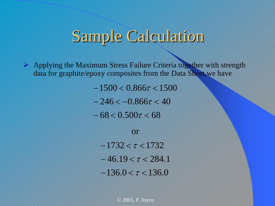
Sample CalculationSample CalculationApplying the Maximum Stress Failure Criteria together with strength data for graphite/epoxy composites from the Data Sheet,we have
68500.06840866.0246
1500866.01500
<<−<−<−<<−
τττ
or
0.1360.1361.28419.46
17321732
<<−<<−
<<−
ττ
τ
© 2003, P. Joyce
Sample CalculationSample CalculationThe off-axis shear strength of a lamina is defined as the minimum of the positive and negative shear stress which can be applied to an angle lamina before failure.Calculations show that τxy = 46.19 MPa is the largest magnitude of shear stress one can apply to the 60° graphite/epoxy composite.However, the largest positive shear stress one could apply is 136.0 MPa, and the largest negative shear stress one could apply is –46.19 MPa.This shows that the maximum magnitude of allowable shear stress in other than the material axes direction depends on the sign of the shear stress.This is because the tensile strength perpendicular to the fiber direction is much lower than the compressive strength perpendicular to the fiber direction.
© 2003, P. Joyce
Failure EnvelopesFailure Envelopes
A failure envelope is a 3D plot of the combinations of normal and shear stresses which can be applied to an angle lamina before failure.Drawing 3D graphs is time consuming. . .One may develop failure envelopes for constant shear stress, τxy, and then use the 2 normal stresses σx and σy as the 2 axes.If the applied stress is within the failure envelope, the lamina is safe; otherwise it has failed.
© 2003, P. Joyce
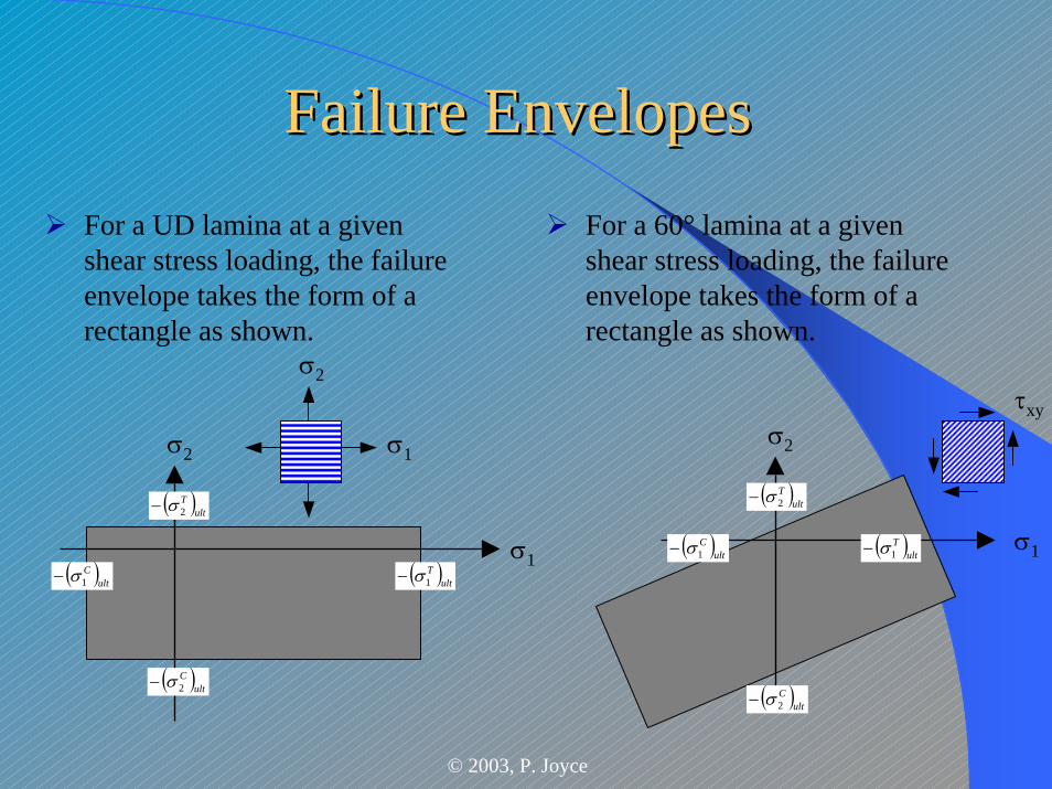
Failure EnvelopesFailure EnvelopesFor a UD lamina at a given shear stress loading, the failure envelope takes the form of a rectangle as shown.
For a 60° lamina at a given shear stress loading, the failure envelope takes the form of a rectangle as shown.
σ2τxy
σ2σ2 σ1
( )ultC1σ− ( )ult
T1σ−
( )ultT2σ−
( )ultC2σ−
( )ultC1σ− ( )ult
T1σ−
( )ultT2σ−
( )ultC2σ−
σ1σ1
© 2003, P. Joyce
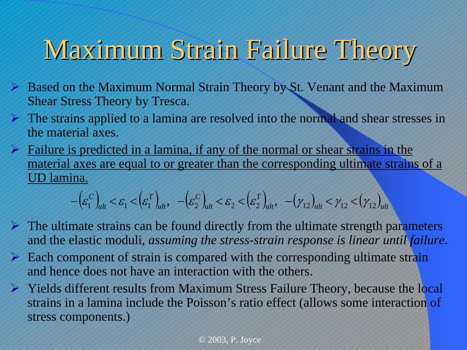
Maximum Strain Failure TheoryMaximum Strain Failure TheoryBased on the Maximum Normal Strain Theory by St. Venant and the Maximum Shear Stress Theory by Tresca.The strains applied to a lamina are resolved into the normal and shear stresses in the material axes.Failure is predicted in a lamina, if any of the normal or shear strains in the material axes are equal to or greater than the corresponding ultimate strains of a UD lamina.
The ultimate strains can be found directly from the ultimate strength parameters and the elastic moduli, assuming the stress-strain response is linear until failure.Each component of strain is compared with the corresponding ultimate strain and hence does not have an interaction with the others.Yields different results from Maximum Stress Failure Theory, because the local strains in a lamina include the Poisson’s ratio effect (allows some interaction of stress components.)
( ) ( ) ( ) ( ) ( ) ( )ultultultT
ultC
ultT
ultC
121212222111 , , γγγεεεεεε <<−<<−<<−
© 2003, P. Joyce
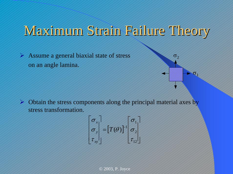
Maximum Strain Failure TheoryMaximum Strain Failure TheoryAssume a general biaxial state of stresson an angle lamina.
Obtain the stress components along the principal material axes by stress transformation.
σ1
σ2
[ ]⎥⎥⎥
⎦
⎤
⎢⎢⎢
⎣
⎡=
⎥⎥⎥
⎦
⎤
⎢⎢⎢
⎣
⎡−
12
2
11)(
τσσ
θτσσ
T
xy
y
x
© 2003, P. Joyce
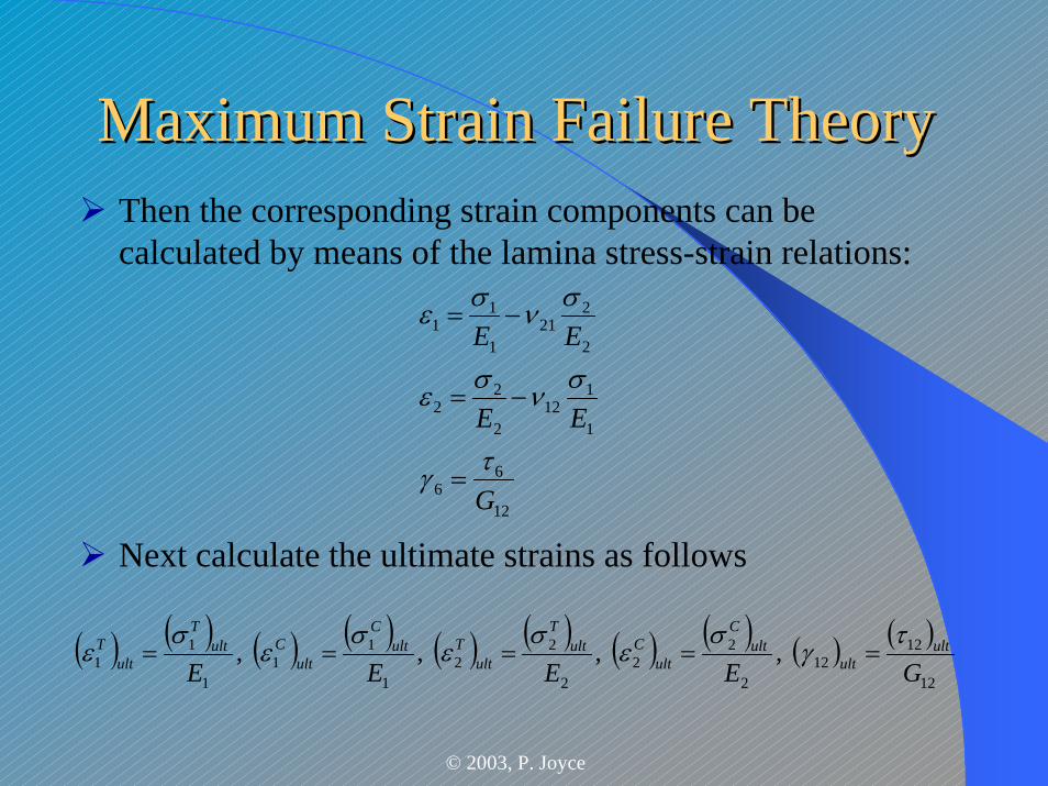
Maximum Strain Failure TheoryMaximum Strain Failure TheoryThen the corresponding strain components can be calculated by means of the lamina stress-strain relations:
Next calculate the ultimate strains as follows12
66
1
112
2
22
2
221
1
11
G
EE
EE
τγ
σνσε
σνσε
=
−=
−=
( ) ( ) ( ) ( ) ( ) ( ) ( ) ( ) ( ) ( )12
1212
2
22
2
22
1
11
1
11 , , , ,
GEEEEult
ultult
C
ultCult
T
ultTult
C
ultCult
T
ultT τ
γσ
εσ
εσ
εσ
ε =====
© 2003, P. Joyce
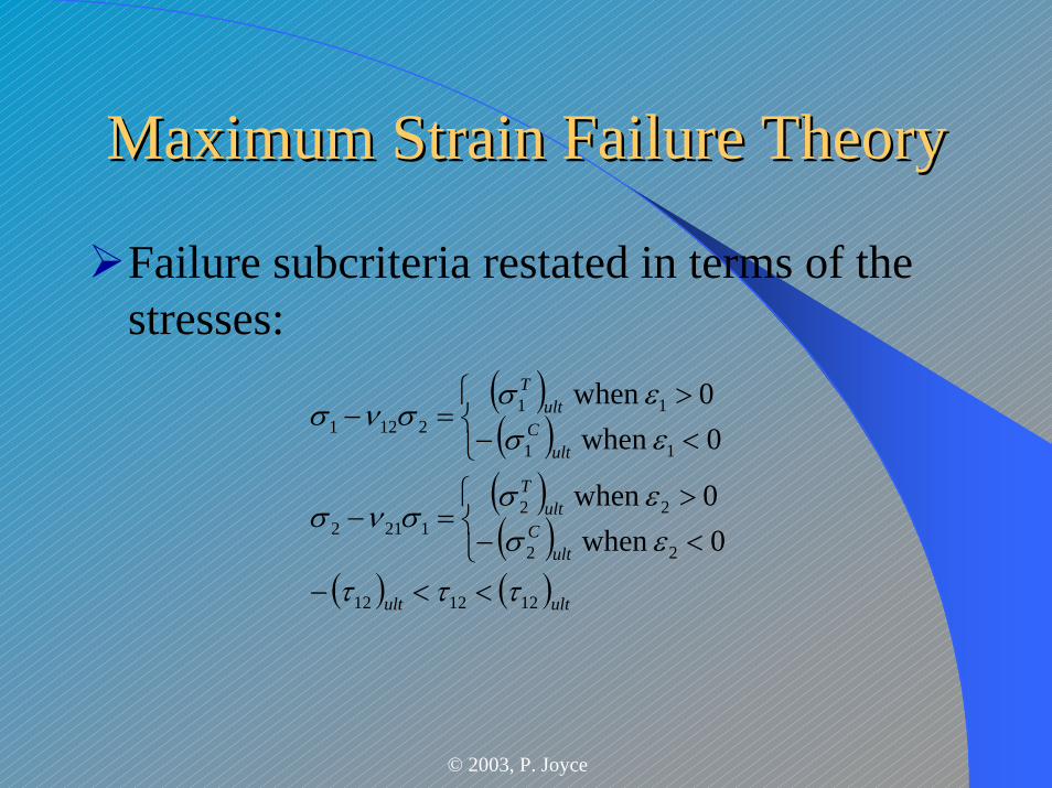
Maximum Strain Failure TheoryMaximum Strain Failure Theory
Failure subcriteria restated in terms of the stresses:
( )( )( )( )
( ) ( )ultult
ultC
ultT
ultC
ultT
121212
22
221212
11
112121
0 when 0 when
0 when 0 when
τττ
εσεσ
σνσ
εσεσ
σνσ
<<−⎩⎨⎧
<−>
=−
⎩⎨⎧
<−>
=−
© 2003, P. Joyce
Maximum Strain Failure TheoryMaximum Strain Failure Theory
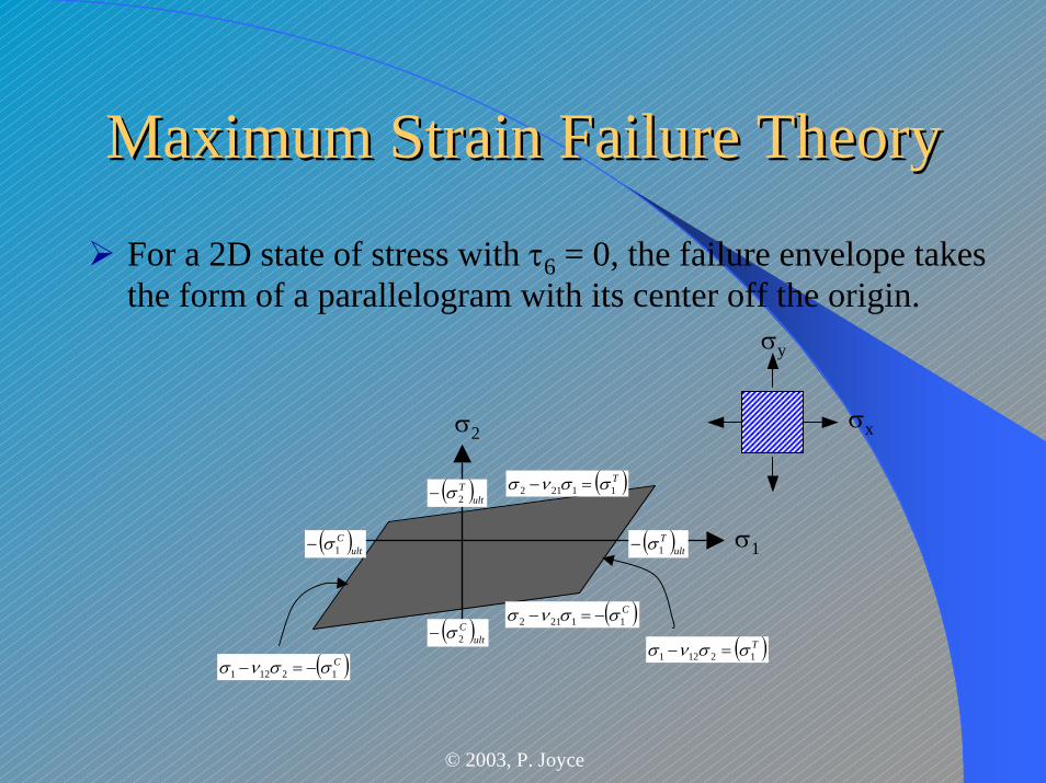
For a 2D state of stress with τ6 = 0, the failure envelope takes the form of a parallelogram with its center off the origin.
σx
σ1
σ2
σy
( )ultC1σ− ( )ult
T1σ−
( )ultT2σ−
( )ultC2σ−
( )C12121 σσνσ −=−
( )T12121 σσνσ =−
( )C11212 σσνσ −=−
( )T11212 σσνσ =−
© 2003, P. Joyce
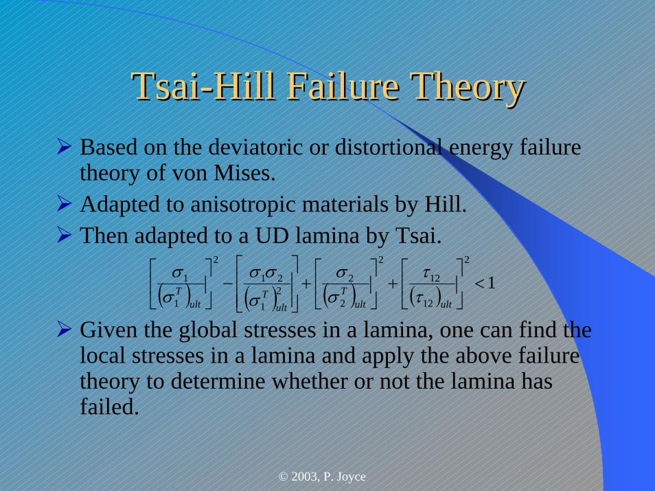
TsaiTsai--Hill Failure TheoryHill Failure TheoryBased on the deviatoric or distortional energy failure theory of von Mises.Adapted to anisotropic materials by Hill.Then adapted to a UD lamina by Tsai.
Given the global stresses in a lamina, one can find the local stresses in a lamina and apply the above failure theory to determine whether or not the lamina has failed.
( ) ( ) ( ) ( ) 12
12
12
2
2
22
1
21
2
1
1 <⎥⎦
⎤⎢⎣
⎡+⎥
⎦
⎤⎢⎣
⎡+
⎥⎥⎦
⎤
⎢⎢⎣
⎡−⎥
⎦
⎤⎢⎣
⎡
ultultT
ultT
ultT τ
τσσ
σσσ
σσ
© 2003, P. Joyce
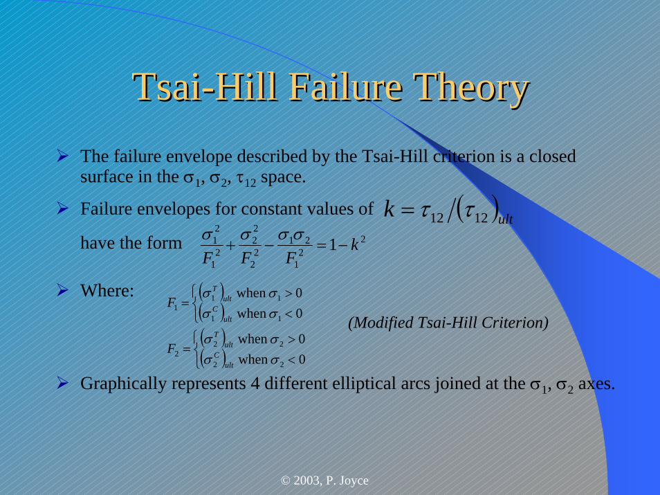
TsaiTsai--Hill Failure TheoryHill Failure TheoryThe failure envelope described by the Tsai-Hill criterion is a closed surface in the σ1, σ2, τ12 space.
Failure envelopes for constant values of
have the form
Where:
Graphically represents 4 different elliptical arcs joined at the σ1, σ2 axes.
( )ultk 1212 ττ=2
21
212
2
22
21
21 1 k
FFF−=−+
σσσσ
( )( )( )( )⎩
⎨⎧
<>
=
⎩⎨⎧
<>
=
0 when 0 when
0 when 0 when
22
222
11
111
σσσσ
σσσσ
ultC
ultT
ultC
ultT
F
F(Modified Tsai-Hill Criterion)
© 2003, P. Joyce
TsaiTsai--Hill Failure TheoryHill Failure Theory
Considers the interaction between the 3 UD lamina strength parameters, unlike the Maximum Stress and Maximum Strain Theories.Tsai-Hill Failure Theory is a Unified Theory and hence does not give the mode of failure like the Maximum Stress and Maximum Strain Theories.
© 2003, P. Joyce
TsaiTsai--Wu Failure TheoryWu Failure Theory
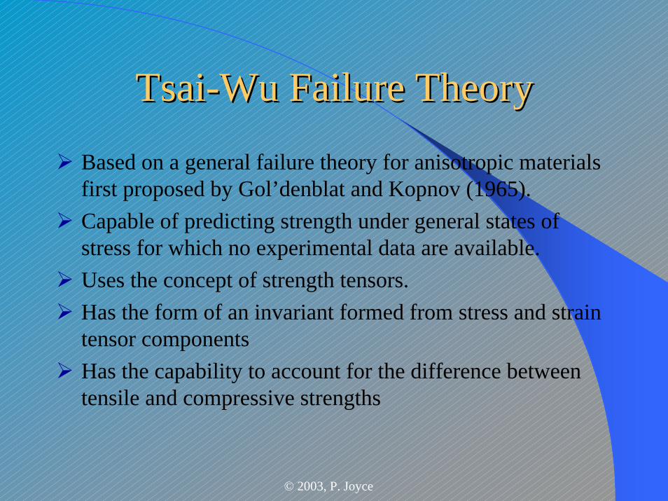
Based on a general failure theory for anisotropic materials first proposed by Gol’denblat and Kopnov (1965).Capable of predicting strength under general states of stress for which no experimental data are available.Uses the concept of strength tensors.Has the form of an invariant formed from stress and strain tensor componentsHas the capability to account for the difference between tensile and compressive strengths
© 2003, P. Joyce
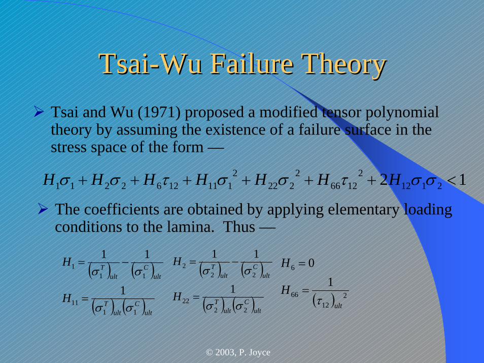
TsaiTsai--Wu Failure TheoryWu Failure TheoryTsai and Wu (1971) proposed a modified tensor polynomial theory by assuming the existence of a failure surface in the stress space of the form —
12 21122
12662
2222
1111262211 <++++++ σστσστσσ HHHHHHH
The coefficients are obtained by applying elementary loading conditions to the lamina. Thus —
( ) ( )
( ) ( )ultC
ultT
ultC
ultT
H
H
1111
111
1
11
σσ
σσ
=
−= ( ) ( )
( ) ( )ultC
ultT
ultC
ultT
H
H
2222
222
1
11
σσ
σσ
=
−=
( ) 212
66
6
10
ult
H
H
τ=
=
© 2003, P. Joyce
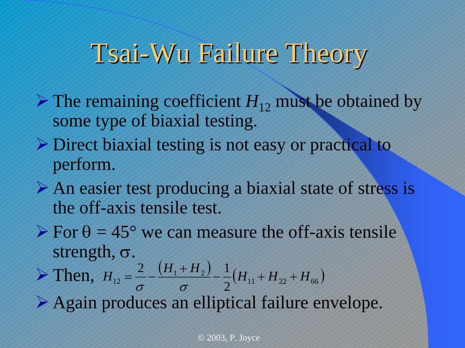
TsaiTsai--Wu Failure TheoryWu Failure TheoryThe remaining coefficient H12 must be obtained by some type of biaxial testing.Direct biaxial testing is not easy or practical to perform.An easier test producing a biaxial state of stress is the off-axis tensile test.For θ = 45° we can measure the off-axis tensile strength, σ.Then,Again produces an elliptical failure envelope.
( ) ( )66221121
12 212 HHHHHH ++−
+−=
σσ
© 2003, P. Joyce
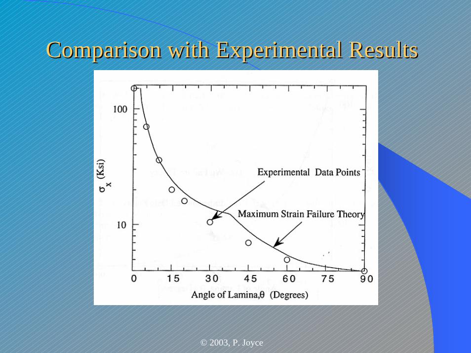
Comparison with Experimental ResultsComparison with Experimental Results
© 2003, P. Joyce
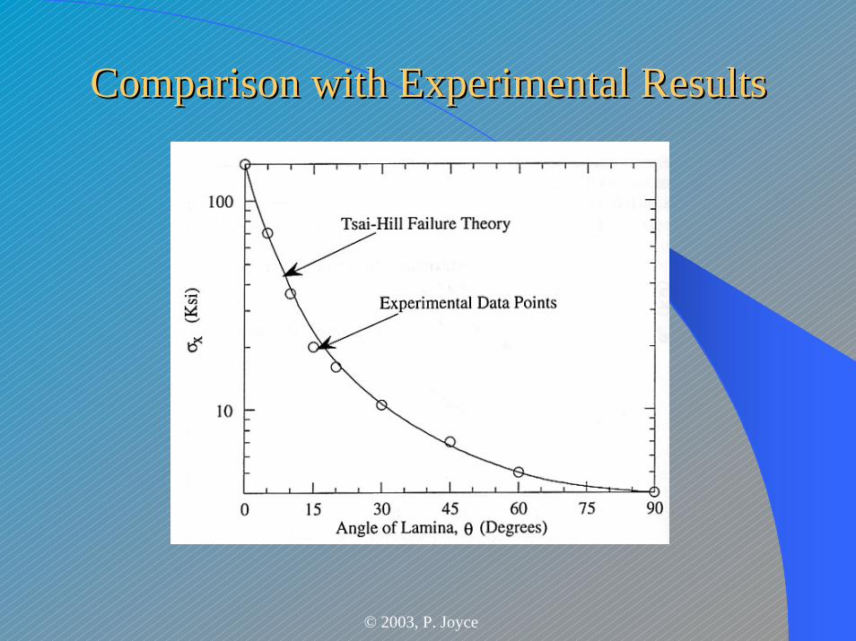
Comparison with Experimental ResultsComparison with Experimental Results
© 2003, P. Joyce
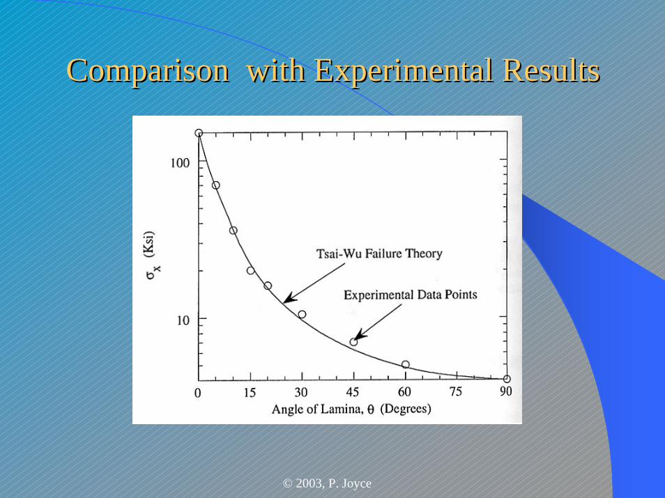
Comparison with Experimental ResultsComparison with Experimental Results
© 2003, P. Joyce
Comparison with Experimental ResultsComparison with Experimental Results
© 2003, P. Joyce
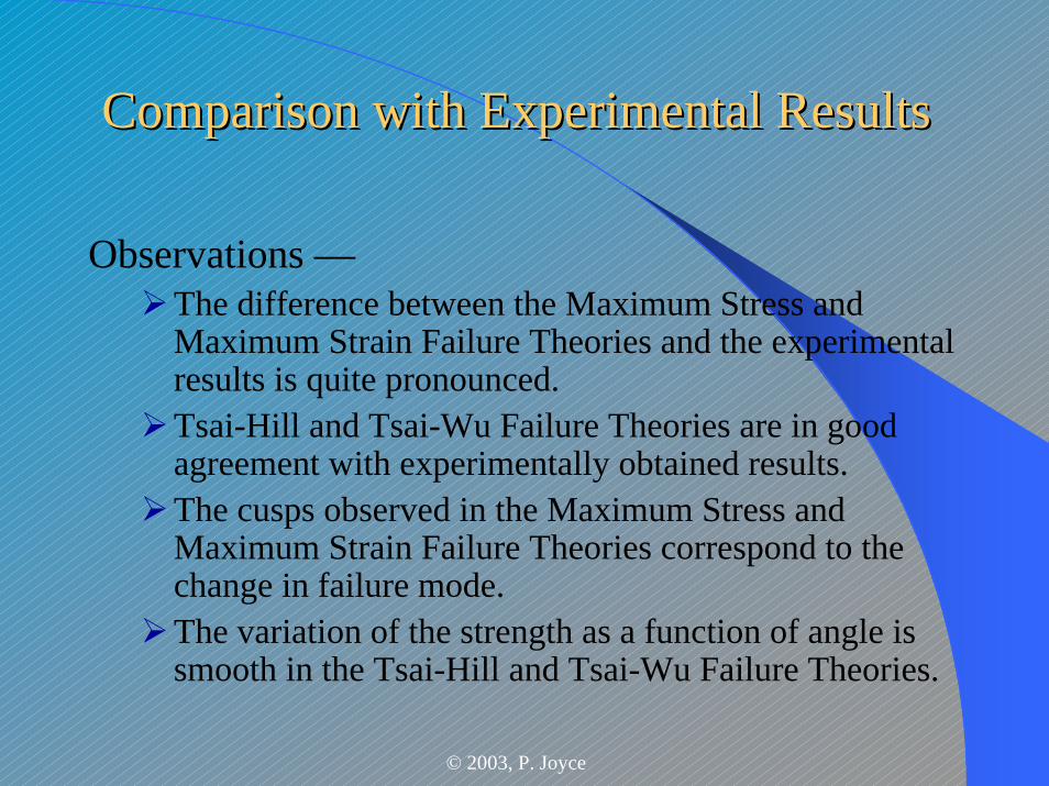
Comparison with Experimental ResultsComparison with Experimental Results
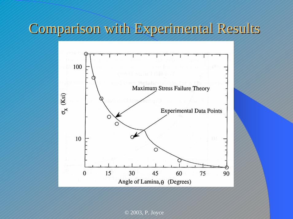
Observations —The difference between the Maximum Stress and Maximum Strain Failure Theories and the experimental results is quite pronounced.Tsai-Hill and Tsai-Wu Failure Theories are in good agreement with experimentally obtained results.The cusps observed in the Maximum Stress and Maximum Strain Failure Theories correspond to the change in failure mode.The variation of the strength as a function of angle is smooth in the Tsai-Hill and Tsai-Wu Failure Theories.
© 2003, P. Joyce
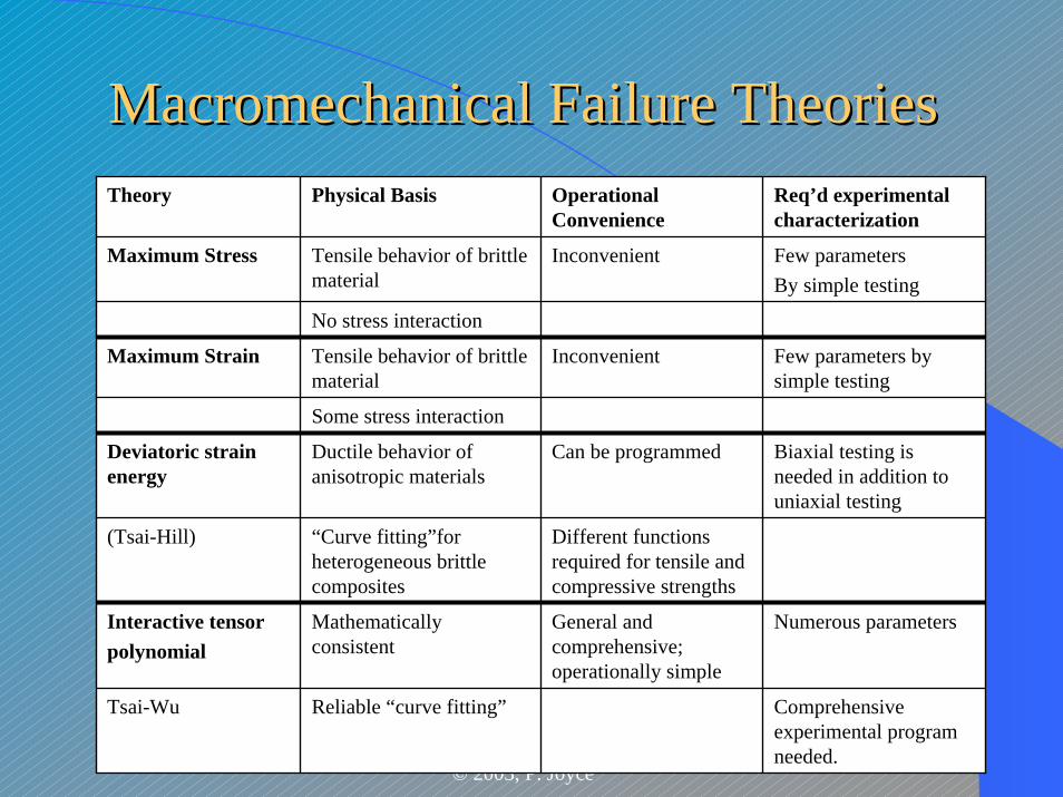
Macromechanical Macromechanical Failure TheoriesFailure TheoriesTheory Physical Basis Operational
ConvenienceReq’d experimental characterization
Maximum Stress Tensile behavior of brittle material
Inconvenient Few parametersBy simple testing
No stress interaction
Maximum Strain Tensile behavior of brittle material
Inconvenient Few parameters by simple testing
Some stress interaction
Deviatoric strain energy
Ductile behavior of anisotropic materials
Can be programmed Biaxial testing is needed in addition to uniaxial testing
(Tsai-Hill) “Curve fitting”for heterogeneous brittle composites
Different functions required for tensile and compressive strengths
Interactive tensorpolynomial
Mathematically consistent
General and comprehensive; operationally simple
Numerous parameters
Tsai-Wu Reliable “curve fitting” Comprehensive experimental program needed.
© 2003, P. Joyce
ReferencesReferencesEngineering Mechanics of Composite Materials, Daniel, I.M. and Ishai, O., 1994.Mechanics of Composite Materials, Kaw, A.K., 1997.Introduction to Composite Materials, Tsai, S. W. and Hahn, H. T., 1980.“Application of Advanced Composites in Mechanical Engineering Designs,” Zweben, C., Proceedings of the 31st International SAMPE Technical Conference, 1999.