SHEAR RHEOMETRY

David Giles and Chris Macosko Department of Chemical Engineering and Materials Science

University of Minnesota 421 Washington Avenue S.E.

Minneapolis MN 55455

http://research.cems.umn.edu/rheology/PolyCharFac.html phone: 612 625 0880 e-mail: giles@umn.edu

1

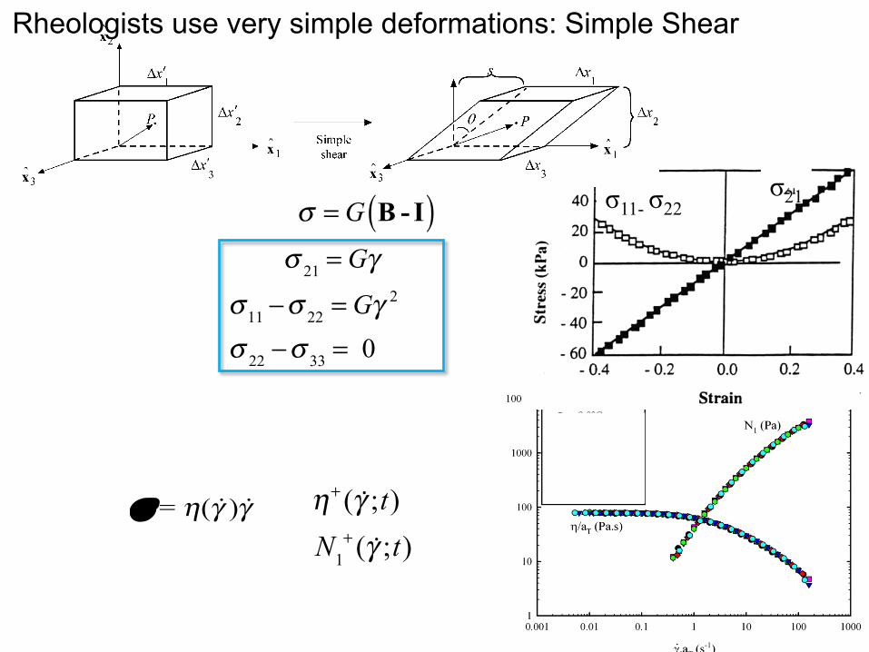
σ = G B - I( ) σ 21 = Gγ

σ 11 −σ 22 = Gγ 2

σ 22 −σ 33 = 0

σ11- σ22

σ21

Rheologists use very simple deformations: Simple Shear

σ =η( !γ ) !γ

η+ ( !γ ;t)N1

+ ( !γ ;t)

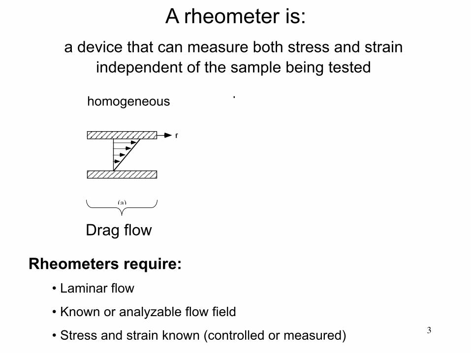
A rheometer is: a device that can measure both stress and strain

independent of the sample being tested

f

p p

(a) (b) (c) !

Drag flow Pressure driven flow

Rheometers require: •  Laminar flow

•  Known or analyzable flow field

•  Stress and strain known (controlled or measured)

homogeneous non-homogeneous

3

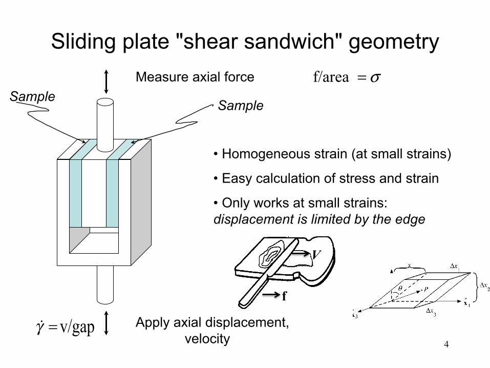
Sliding plate "shear sandwich" geometry

Apply axial displacement, velocity

Measure axial force

• Homogeneous strain (at small strains)

• Easy calculation of stress and strain

• Only works at small strains: displacement is limited by the edge

Sample Sample

4 !γ =

f/area σ=

v/gap

f

V

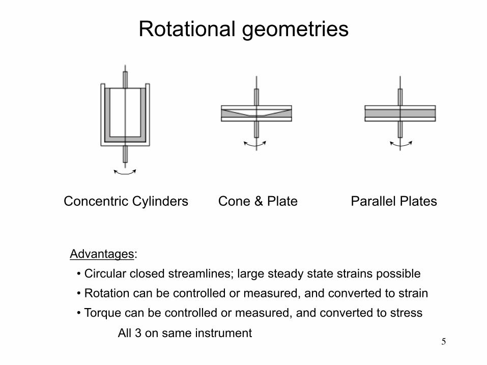
Rotational geometries

Cone & Plate Concentric Cylinders Parallel Plates

Advantages: • Circular closed streamlines; large steady state strains possible • Rotation can be controlled or measured, and converted to strain • Torque can be controlled or measured, and converted to stress

All 3 on same instrument

5

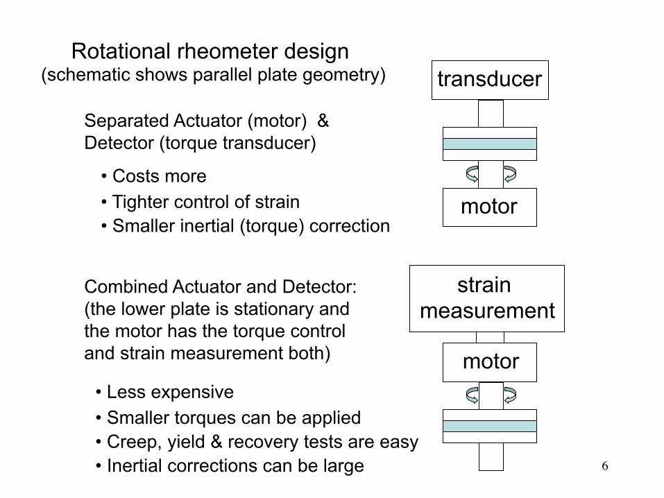
Rotational rheometer design (schematic shows parallel plate geometry)

Separated Actuator (motor) & Detector (torque transducer)

Combined Actuator and Detector: (the lower plate is stationary and the motor has the torque control and strain measurement both)

motor

transducer

strain measurement

motor • Less expensive • Smaller torques can be applied • Creep, yield & recovery tests are easy • Inertial corrections can be large

• Costs more • Tighter control of strain • Smaller inertial (torque) correction

6

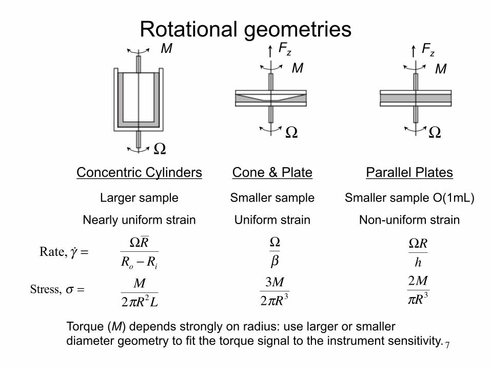
Rotational geometries

Cone & Plate

Smaller sample

Uniform strain

�

Ωβ3M2πR3

Concentric Cylinders

Larger sample

Nearly uniform strain

�

ΩR Ro − Ri

M2πR2L

Parallel Plates

Smaller sample O(1mL)

Non-uniform strain

�

ΩRh2MπR3

=γ Rate,

Stress, σ =

Torque (M) depends strongly on radius: use larger or smaller diameter geometry to fit the torque signal to the instrument sensitivity.

Ω

MM

Fz M

Fz

Ω Ω

7

Couette (concentric cylinders) geometry, rotational rheometry:

Typical sample size

~ 10 mL

Ω

L

2Ro2Ri

Sample

Shear stress = ForceArea

= Torque/Radius2πRL

= Torque2πR2L

= M2πR2L

�

Shear stress = Torque2πRi

2L on the inner cylinder

�

Shear rate ≅ ΔvΔr

= ΩR Ro − Ri�

Shear stress = Torque2πRo

2L on the outer cylinder

�

differ by RiRo

⎛

⎝ ⎜

⎞

⎠ ⎟

2

�

"Narrow gap"⇒κ = RiRo

≥ 0.998

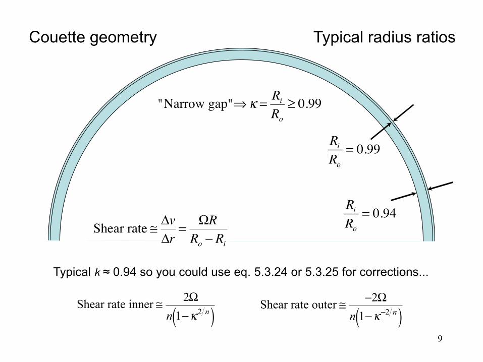
Couette geometry Typical radius ratios

Typical k ≈ 0.94 so you could use eq. 5.3.24 or 5.3.25 for corrections...

�

"Narrow gap"⇒κ = RiRo

≥ 0.99

�

Shear rate ≅ ΔvΔr

= ΩR Ro − Ri

�

Shear rate inner ≅ 2Ωn 1−κ2 n( )

�

Shear rate outer ≅ −2Ωn 1−κ−2 n( )

RiRo

= 0.99

RiRo

= 0.94

9

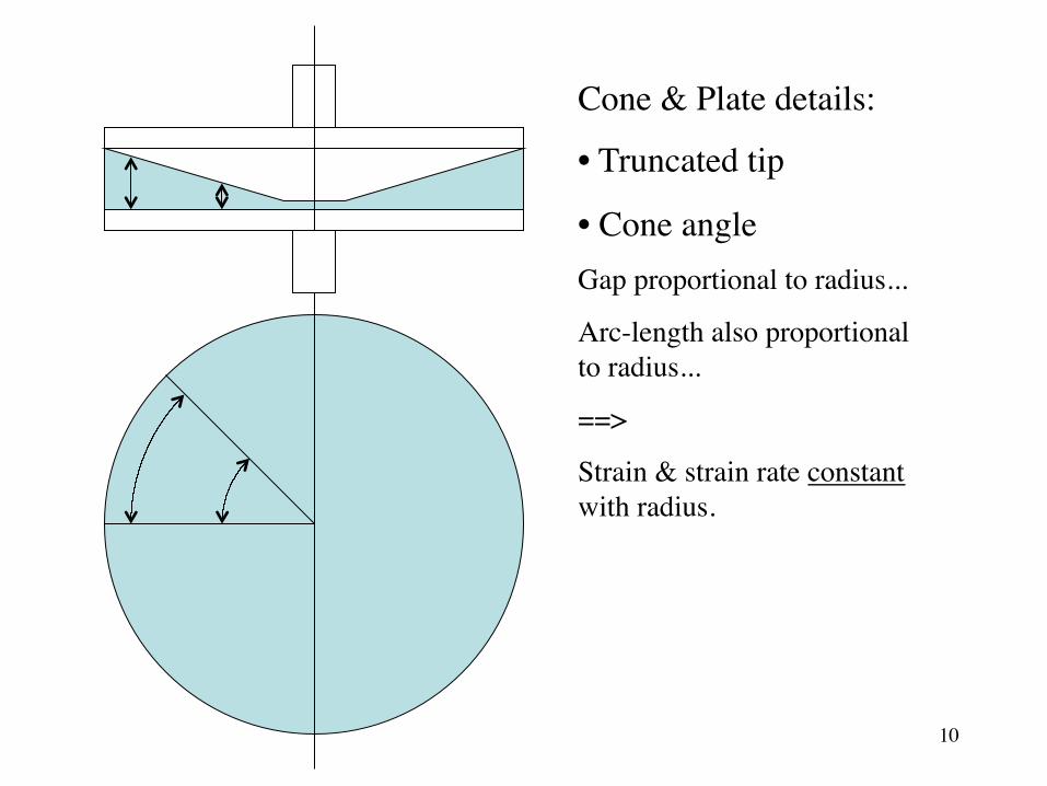
Cone & Plate details:

• Truncated tip

• Cone angleGap proportional to radius...

Arc-length also proportional to radius...

==>

Strain & strain rate constant with radius.

10

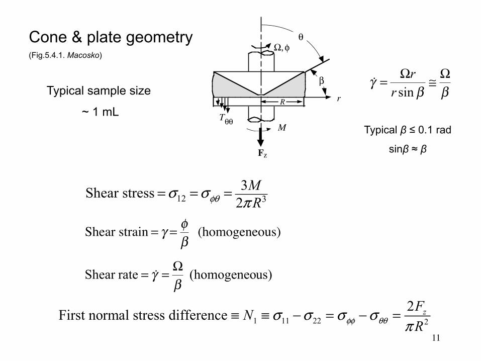
Cone & plate geometry (Fig.5.4.1. Macosko)

Typical sample size

~ 1 mL

12 33Shear stress

2MRφθσ σ

π= = =

�

Shear strain = γ = φβ

(homogeneous)

1 11 22 2

2First normal stress difference zFNRφφ θθσ σ σ σ

π≡ ≡ − = − =

r

Ω, φ

M

R

θ

T

Fz

θθ

βββ

γ Ω≅Ω=sinrr

us)(homogeneo rateShear β

γ Ω==

Typical β ≤ 0.1 rad

sinβ ≈ β

11

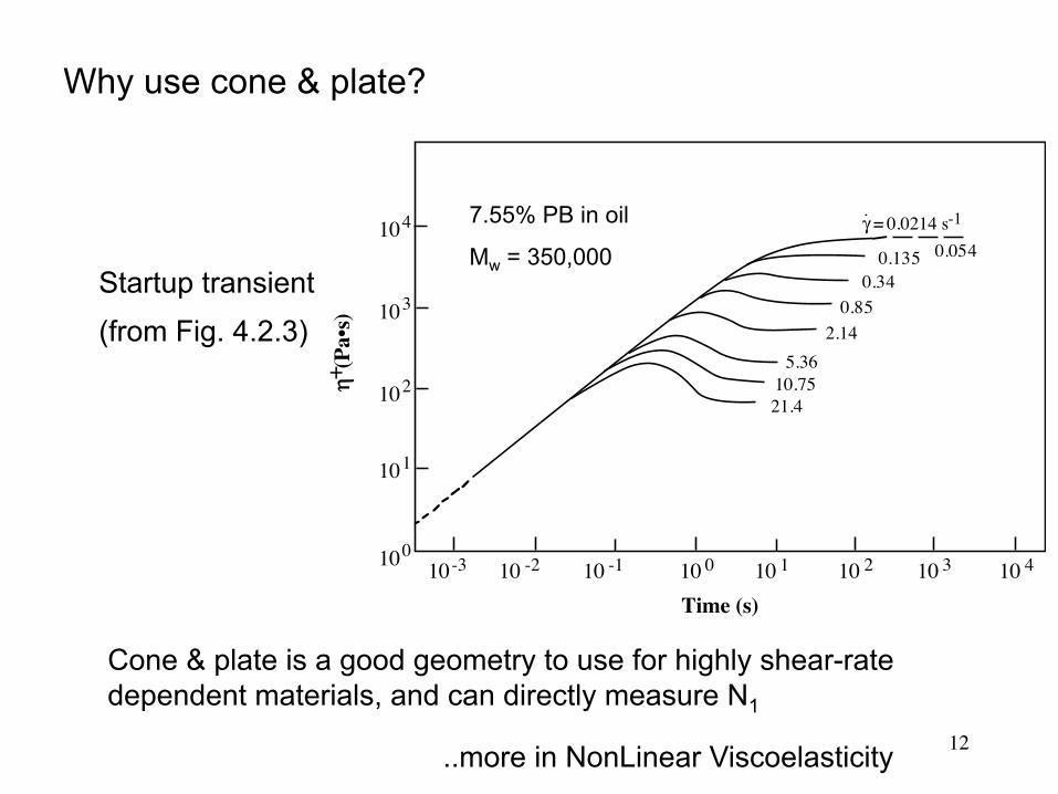
Why use cone & plate?

+ η (P

a•s)

10-3 10 0

Time (s)10 -2 10 -1 10 1 10 2 10 3 10 4100

101

102

103

104 γ = 0.0214 s-1

0.050.130.3

0.82.14

5.3610.7521.4

454

5Startup transient (from Fig. 4.2.3)

Cone & plate is a good geometry to use for highly shear-rate dependent materials, and can directly measure N1

12

7.55% PB in oil

Mw = 350,000

..more in NonLinear Viscoelasticity

Normal stress effects Weissenberg (rod climbing)

1 11 22 2

2First normal stress difference zFNRφφ θθσ σ σ σ

π≡ ≡ − = − =

Die swell (extrudate swell)

Newtonian (glycerin)

Polymer Solution (glycerin &

polyacrylamide)

Polymer melts and entangled solutions swell when exiting a die

(cone & plate)

(pictures from Dynamics of Polymeric Liquids, Volume 1; Bird, Armstrong, and Hassager)

13

Add some applications of N1. difficulties in meauring

Parallel plate geometry (Fig.5.5.1. Macosko)

Typical sample size

~ 1 mL

σπ

= = 32Shearstress (correctforNewtonian)MR

Shear strain = γ r( ) = θrh

(non-homogeneous strain, depends on r)

( ) ⎥⎦

⎤⎢⎣

⎡ +=−R

zz FRFNN

R γ∂∂

πγ loglog2221

! !γ =!θrh= Ωrh

!! Nominal!shear!rate= !γ R =

ΩRh!!(calculated!at!r=R)

Ω, θ

M

R

F

h

z

Shear stress =σ = M

2πR3 3+∂ log M∂ log !γ R

⎡

⎣⎢

⎤

⎦⎥

Corrected for non- Newtonian material

14

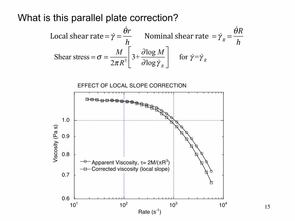
What is this parallel plate correction?

!! Local!shear!rate= !γ =

!θrh!!!!!!!Nominal!shear!rate! = !γ R =

!θRh

Shear stress =σ = M

2πR3 3+∂ log M∂ log !γ R

⎡

⎣⎢

⎤

⎦⎥ for !γ = !γ R

0.6

0.7

0.8

0.9

1.0

101 102 103 104

EFFECT OF LOCAL SLOPE CORRECTION (LP solution)

Apparent Viscosity, τ= 2M/(πR3)Corrected viscosity (local slope)

Visc

osity

(Pa

s)

Rate (s-1)15

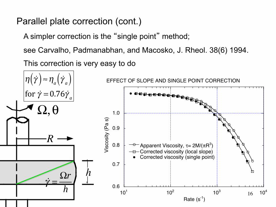
Parallel plate correction (cont.) A simpler correction is the “single point” method;

see Carvalho, Padmanabhan, and Macosko, J. Rheol. 38(6) 1994.

0.6

0.7

0.8

0.9

1.0

101 102 103 104

EFFECT OF SLOPE AND SINGLE POINT CORRECTION (LP solution)

Apparent Viscosity, τ= 2M/(πR3)Corrected viscosity (local slope)Corrected viscosity (single point)

Visc

osity

(Pa

s)

Rate (s-1)16

This correction is very easy to do

Ω, θ

M

R

F

h

z

!!

η !γ( )≈ηa!γ a( )

for! !γ =0.76 !γ a

! !γ = Ωr

h

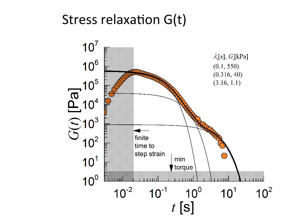
Stressrelaxa*onG(t)

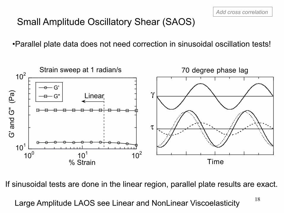
Small Amplitude Oscillatory Shear (SAOS)

• Parallel plate data does not need correction in sinusoidal oscillation tests!

70 degree phase lag

Time

γ

τ

101

102

100 101 102

Strain sweep at 1 radian/s

G'G"

G' a

nd G

" (P

a)

% Strain

Linear

If sinusoidal tests are done in the linear region, parallel plate results are exact.

18Large Amplitude LAOS see Linear and NonLinear Viscoelasticity

Add cross correlation

Cox-Merz rule: Compare dynamic (sinusoidal) and steady-shear viscosity:

�

η∗ versus frequency (radians/s)η versus shear rate (1/s)compare

Cox-Merz works great for linear polymers! Not for crosslinked materials, most suspensions, materials with structure that is too fundamentally changed by (large) steady shearing.

For these, steady or dynamic can be useful, but each in it’s own way 100

101

102

10-2 10-1 100 101 102

NIST solution, steady and sinusoidal compared

Dyn Freq Swp

Steady Rate Sweep

Stea

dy S

hear

or C

ompl

ex V

isco

sity

(Pa

s)

Frequency (rad/s) or Rate (s-1)19

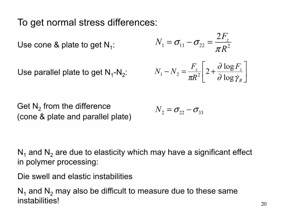
To get normal stress differences:

Use cone & plate to get N1:

Get N2 from the difference (cone & plate and parallel plate)

1 11 22 2

2 zFNR

σ σπ

= − =

Use parallel plate to get N1-N2:

2 22 33N σ σ= −

⎥⎦

⎤⎢⎣

⎡ +=−R

zz FRFNN

γ∂∂

π loglog2221

N1 and N2 are due to elasticity which may have a significant effect in polymer processing:

Die swell and elastic instabilities

N1 and N2 may also be difficult to measure due to these same instabilities! 20

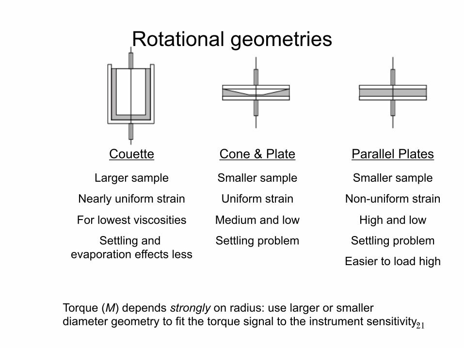
Rotational geometries

Cone & Plate

Smaller sample

Uniform strain

Medium and low

Settling problem

Couette

Larger sample

Nearly uniform strain

For lowest viscosities

Settling and evaporation effects less

Parallel Plates

Smaller sample

Non-uniform strain

High and low

Settling problem

Easier to load high

Torque (M) depends strongly on radius: use larger or smaller diameter geometry to fit the torque signal to the instrument sensitivity. 21

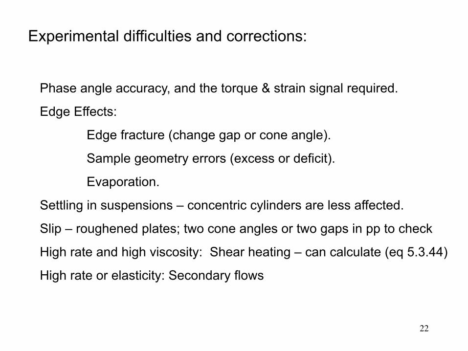
Experimental difficulties and corrections:

Phase angle accuracy, and the torque & strain signal required.

Edge Effects:

Edge fracture (change gap or cone angle).

Sample geometry errors (excess or deficit).

Evaporation.

Settling in suspensions – concentric cylinders are less affected.

Slip – roughened plates; two cone angles or two gaps in pp to check

High rate and high viscosity: Shear heating – can calculate (eq 5.3.44)

High rate or elasticity: Secondary flows

22

SAOS sensitivity: phase angle resolution...

Velankar and Giles, Rheology Bulletin, 2007

frequency ω (rad/s)0.01 0.1 1 10 100

G', G

" (Pa)

10-2

10-1

100

101

102

103

104

105

10% strain1% 0.1% strain sweep below

fit region

0.001

0.01

0.1

1

10

0.1 1 10 100frequency ω (rad/s)

stra

in π

min

%

minimum strainfor 5% error

measurements inaccurate

measurements accurate

1.8

2

2.2

2.4

2.6

0.01 0.1 1 10 100 1000strain γ %

log

(tan

⎝)

0.32 rad/s0.56 rad/s1rad/s

γmin added to graph on right

+/- 5% error

plateau values added as red points

to graph above

(Nearly monodisperse polyisoprene melt)

23

SAOS sensitivity: phase angle resolution...

Velankar and Giles, Rheology Bulletin, 2007

0.001

0.01

0.1

1

10

0.1 1 10 100frequency ω (rad/s)

stra

in π

min

%

minimum strainfor 5% error

measurements inaccurate

measurements accurate

The minimum torque or displacement for accurate phase angle resolution may be much greater than that specified by the manufacturer!

(Nearly monodisperse polyisoprene melt)

24

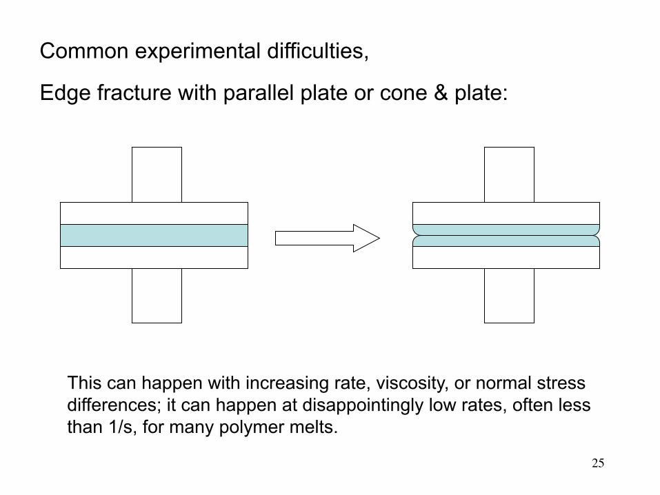
Common experimental difficulties,

Edge fracture with parallel plate or cone & plate:

This can happen with increasing rate, viscosity, or normal stress differences; it can happen at disappointingly low rates, often less than 1/s, for many polymer melts.

25

26

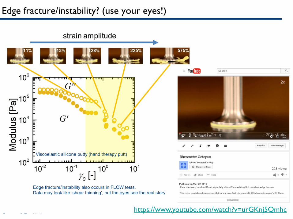
Edge fracture/instability? (use your eyes!)

��https://www.youtube.com/watch?v=urGKnj5Qmhc

9LVFRHODVWLF�VLOLFRQH�SXWW\��KDQG�WKHUDS\�SXWW�

(GJH�IUDFWXUH�LQVWDELOLW\�DOVR�RFFXUV�LQ�)/2:�WHVWV��'DWD�PD\�ORRN�OLNH�µVKHDU�WKLQQLQJ¶��EXW�WKH�H\HV�VHH�WKH�UHDO�VWRU\

&RUPDQ��(ZROGW��in prep

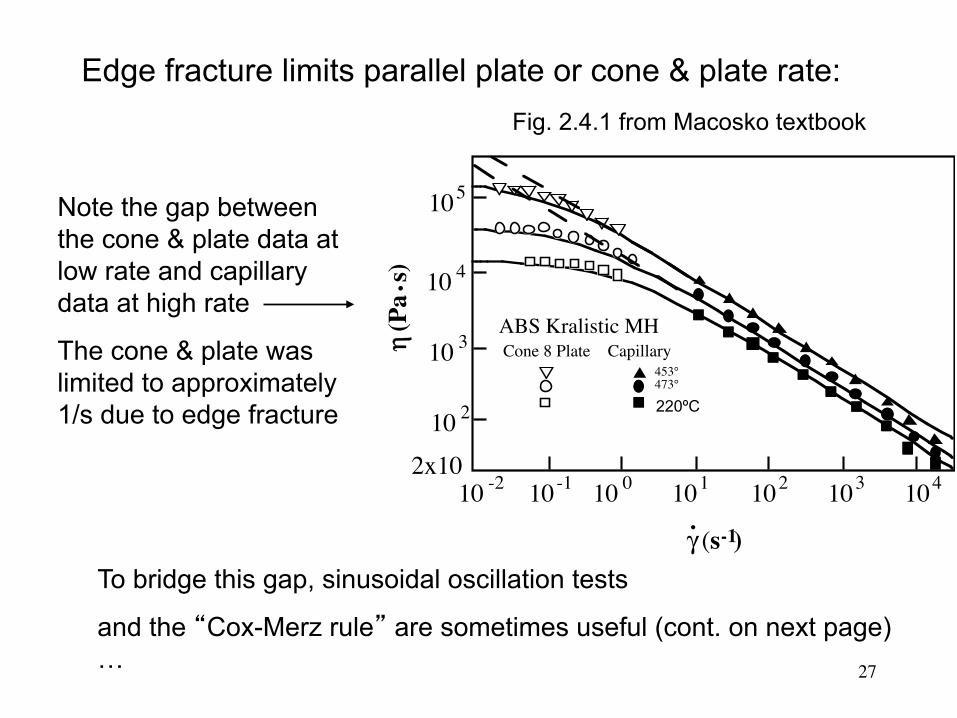
Fig. 2.4.1 from Macosko textbook

To bridge this gap, sinusoidal oscillation tests

and the “Cox-Merz rule” are sometimes useful (cont. on next page)…

105

10 4

10 3

10 2

2x1010 -2 10-1 10 0 101 102 103 104

ABS Kralistic MHCone 8 Plate Capillary

453°473°493°

γ (s-1)

η (P

a s)

Note the gap between the cone & plate data at low rate and capillary data at high rate

The cone & plate was limited to approximately 1/s due to edge fracture

Edge fracture limits parallel plate or cone & plate rate:

27

220ºC

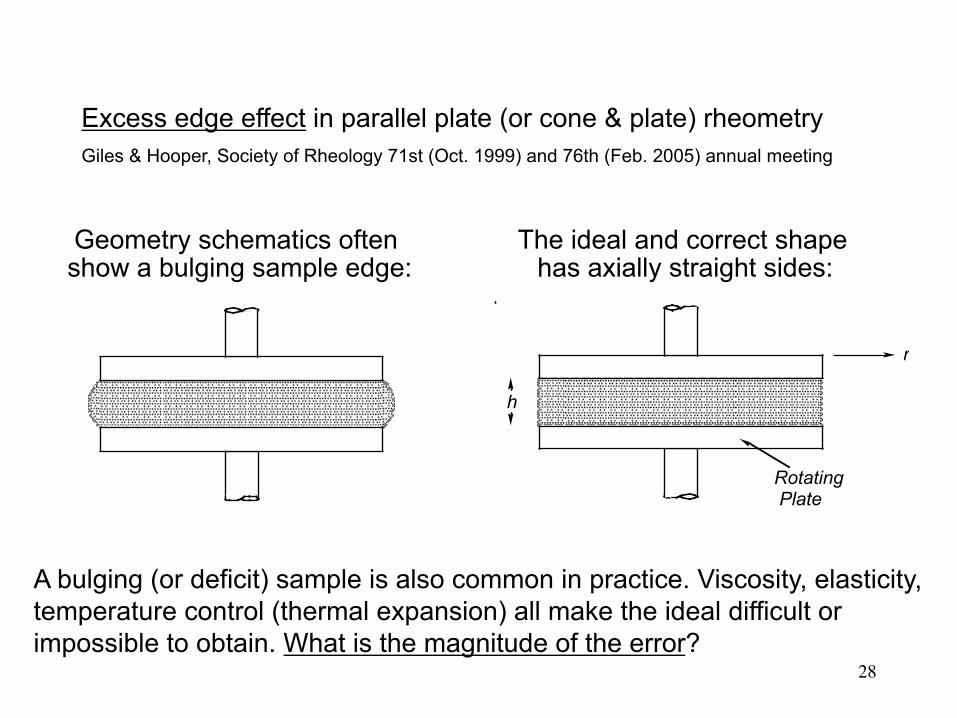
Excess edge effect in parallel plate (or cone & plate) rheometry Giles & Hooper, Society of Rheology 71st (Oct. 1999) and 76th (Feb. 2005) annual meeting

A bulging (or deficit) sample is also common in practice. Viscosity, elasticity, temperature control (thermal expansion) all make the ideal difficult or impossible to obtain. What is the magnitude of the error?

h

r

Rotating Plate

Geometry schematics often show a bulging sample edge:

The ideal and correct shape has axially straight sides:

28

Excess edge effect, other typical shapes:

h

2Rδ

2(R+δ)

Axially straight sample edges are impossible with a larger lower plate. Contact angles and amount of excess can vary; δ = h could be typical.

2Rδ

�

MM0

= 1+ C HR⎛

⎝ ⎜

⎞

⎠ ⎟

Hemisphere excess disk

C = 0.85

For δ = h/2

Minimally wetted large lower plate

C = 1.1 for δ = h

Excess edge effect

29

For “sea of fluid” C = 1.9

End effect correction with concentric cylinders: Giles et al., Society of Rheology, 83rd (Oct. 2011) annual meeting

The correction is 5%-10% when the annular gap is kept reasonably small relative to the bob radius, and the bob length is three times the radius

30

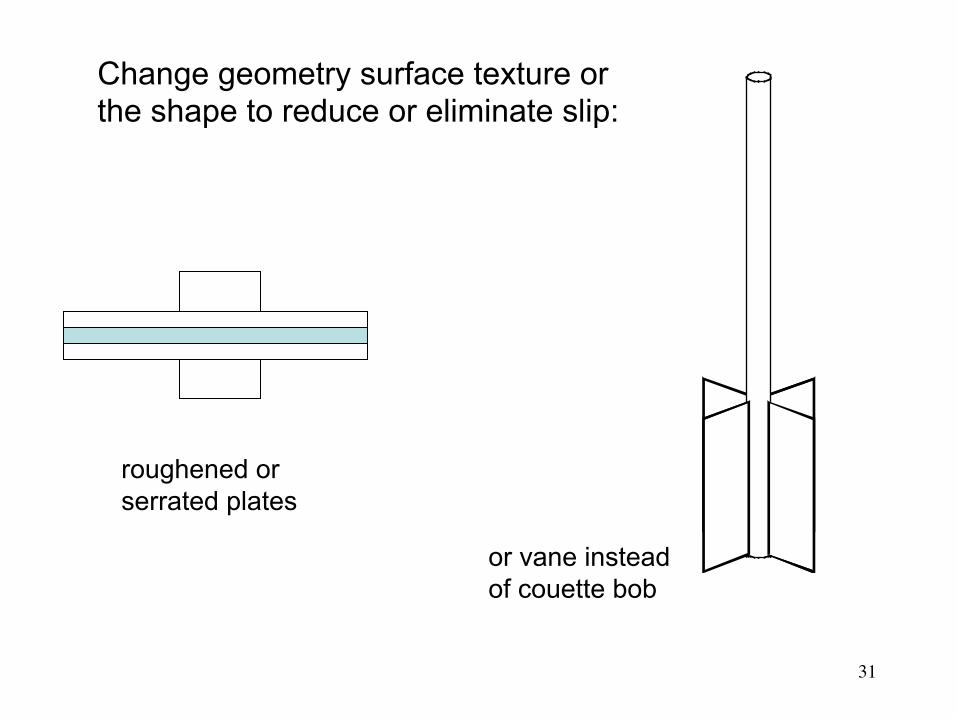
Change geometry surface texture or the shape to reduce or eliminate slip:

roughened or serrated plates

or vane instead of couette bob

31

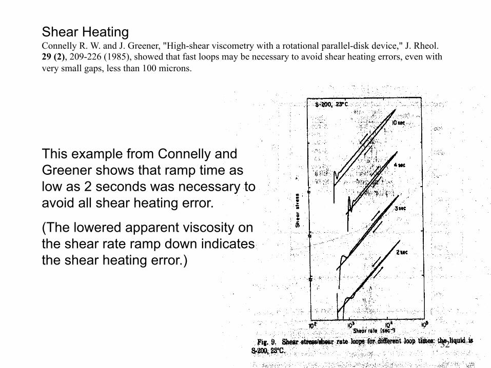
Shear Heating Connelly R. W. and J. Greener, "High-shear viscometry with a rotational parallel-disk device," J. Rheol. 29 (2), 209-226 (1985), showed that fast loops may be necessary to avoid shear heating errors, even with very small gaps, less than 100 microns.

This example from Connelly and Greener shows that ramp time as low as 2 seconds was necessary to avoid all shear heating error.

(The lowered apparent viscosity on the shear rate ramp down indicates the shear heating error.)

32

At small gaps there is usually a gap error that needs to be corrected.

Connelly and Greener, J. of Rheol., 29(2) 1985

Plates not completely clean during zeroing

Non-parallelism 33

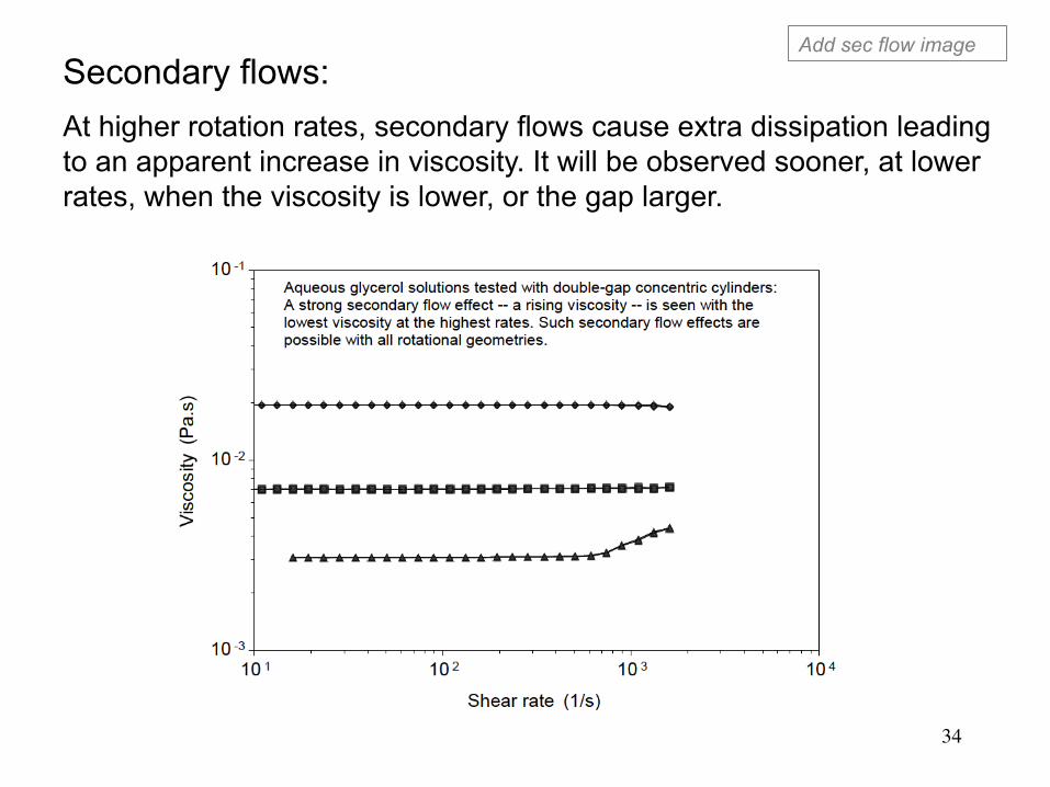
Secondary flows: At higher rotation rates, secondary flows cause extra dissipation leading to an apparent increase in viscosity. It will be observed sooner, at lower rates, when the viscosity is lower, or the gap larger.

34

Add sec flow image

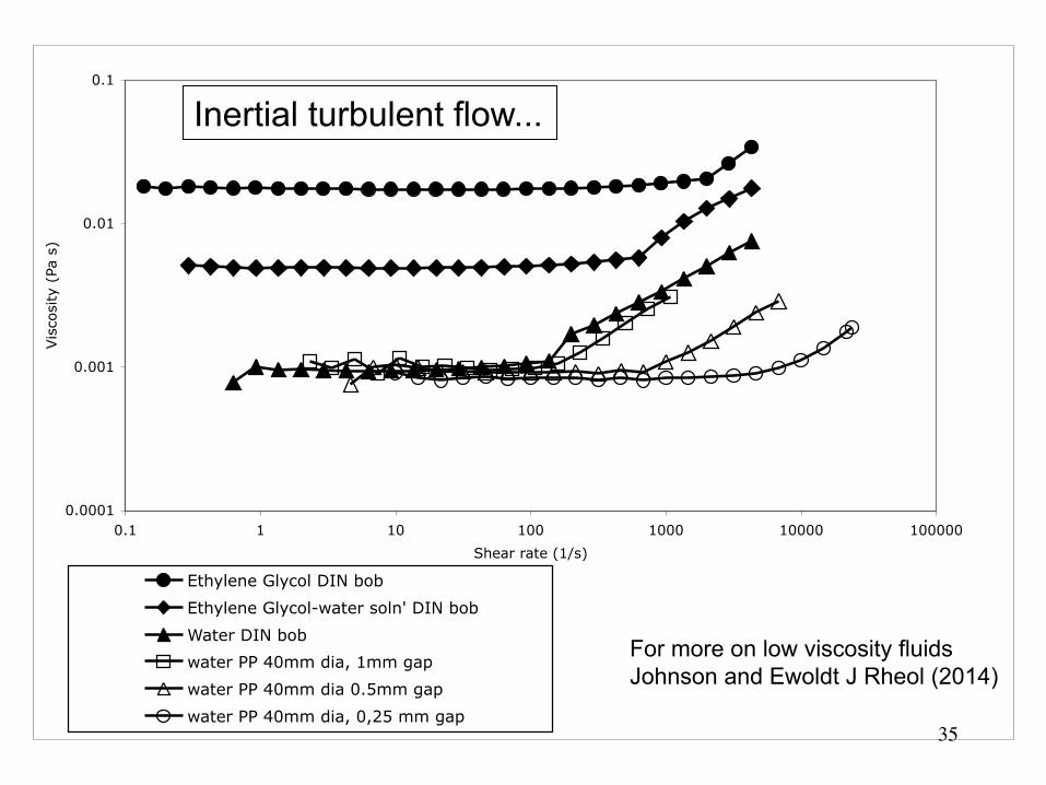
0.0001

0.001

0.01

0.1

0.1 1 10 100 1000 10000 100000

Shear rate (1/s)

Vis

cosi

ty (

Pa s

)

Ethylene Glycol DIN bob

Ethylene Glycol-water soln' DIN bob

Water DIN bob

water PP 40mm dia, 1mm gap

water PP 40mm dia 0.5mm gap

water PP 40mm dia, 0,25 mm gap

Inertial turbulent flow...

35

For more on low viscosity fluids Johnson and Ewoldt J Rheol (2014)

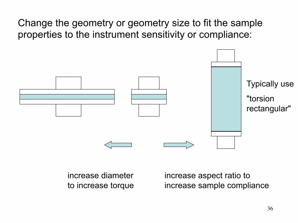
Change the geometry or geometry size to fit the sample properties to the instrument sensitivity or compliance:

increase diameter to increase torque

increase aspect ratio to increase sample compliance

Typically use

"torsion rectangular"

36

37

Ideal definitions versus reality of experiments

��

An incomplete list of non-ideal effects:

(A) Resolution/range of measured load and displacement

(B) Instrument inertia (if load and displacement are measured on same boundary)

(C) Fluid inertia and secondary flows

(D) Surface tension

(E) Free surface interfacial rheology

(F) Slip at boundaries

(G) Sample underfill or overfill

(H) Small volume and gap

(I) Non-homogenous sample from settling, migration, or rheotaxis

(J) …and more…this requires thinking about the entire system used for the measurement, and what may be non-ideal. (viscous heating? thermal gradients? transducer drift?...)

38

Other resources on avoiding bad data

�

7$7HFK7LSVKWWSV���ZZZ�\RXWXEH�FRP�XVHU�7$7HFK7LSV

$QWRQ�3DDU H/HDUQLQJKWWSV���ZZZ�\RXWXEH�FRP�XVHU�$QWRQ3DDU+4�SOD\OLVWV

Other resources on avoiding bad data

�

7$7HFK7LSVKWWSV���ZZZ�\RXWXEH�FRP�XVHU�7$7HFK7LSV

$QWRQ�3DDU H/HDUQLQJKWWSV���ZZZ�\RXWXEH�FRP�XVHU�$QWRQ3DDU+4�SOD\OLVWV

�

�

www.youtube.com/watch?v=1cymypBsEzM

39

1. co-plot experimental boundaries on data2. compare different geometries3. look at data for key signatures of bad data4. look at experiment, take photos/videos

��

4 BIG IDEAS FOR CHECKING YOUR DATAChecks for Bad Data

Big Idea #3: look for key signatures of bad (non-ideal) data

��

6LJQDWXUHV�RI�QRQ�LGHDO�GDWD� 6FDWWHU� &RQVWDQW�WRUTXH�RIIVHW� +LJK�IUHTXHQF\�XSWXUQ� +LJK�UDWH�XSWXUQ� 5LQJLQJ� 7UDQVLHQW�DFFHOHUDWLRQ� *DS�GHSHQGHQFH

Big Idea #3: look for key signatures of bad (non-ideal) data

��

6LJQDWXUHV�RI�QRQ�LGHDO�GDWD� 6FDWWHU� &RQVWDQW�WRUTXH�RIIVHW� +LJK�IUHTXHQF\�XSWXUQ� +LJK�UDWH�XSWXUQ� 5LQJLQJ� 7UDQVLHQW�DFFHOHUDWLRQ� *DS�GHSHQGHQFH

Big Idea #2: when in doubt, measure with different geometries

��

7UXH�³,QWULQVLF´�PDWHULDO�SURSHUWLHV�DUH�LQGHSHQGHQW�RI�JHRPHWU\

&RPPRQ�RSWLRQV�WR�FKDQJH�JHRPHWU\�� &KDQJH�JDS� 5RXJK�versus VPRRWK�VXUIDFHV� (OLPLQDWH�IUHH�VXUIDFH� &RQH�versus SODWH�versus FRQFHQWULF�

F\OLQGHU

³([WULQVLF´�SURSHUWLHV�PD\�VWLOO�EH�UHOHYDQW�IRU�\RXU�UKHRORJLFDOO\�FRPSOH[�PDWHULDO��H�J��JUDQXODU�PDWHULDOV��QRQ�FRQWLQXXP�OHQJWKVFDOHV��ZDOO�VOLS�

6KDUPD�HW�DO��6RIW�0DWWHU����� 0DJGD��/DUVRQ�-11)0�����

40

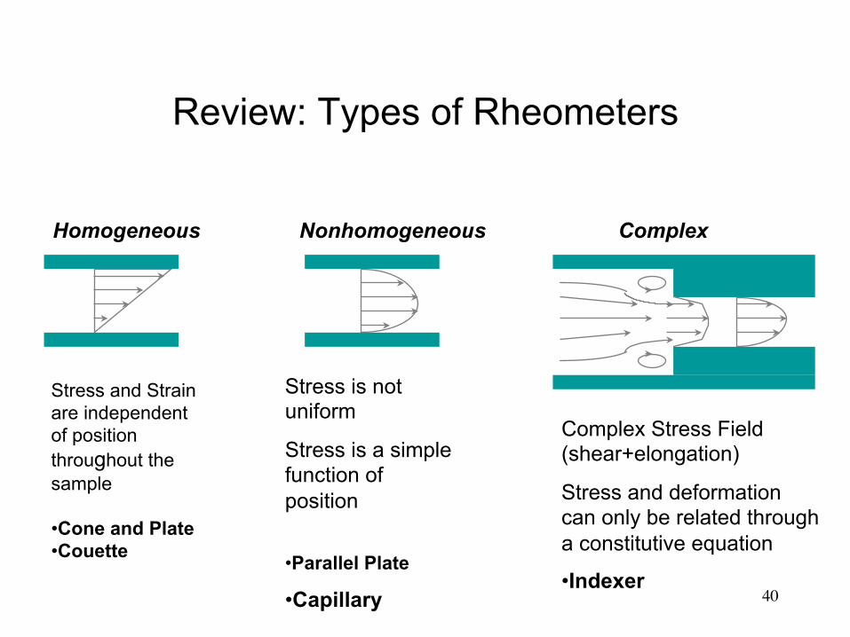
Review: Types of Rheometers

Stress and Strain

are independent of position throughout the sample • Cone and Plate • Couette

Homogeneous Nonhomogeneous

Stress is not uniform

Stress is a simple function of position

• Parallel Plate

• Capillary

Complex

Complex Stress Field (shear+elongation)

Stress and deformation can only be related through a constitutive equation

• Indexer

6-41

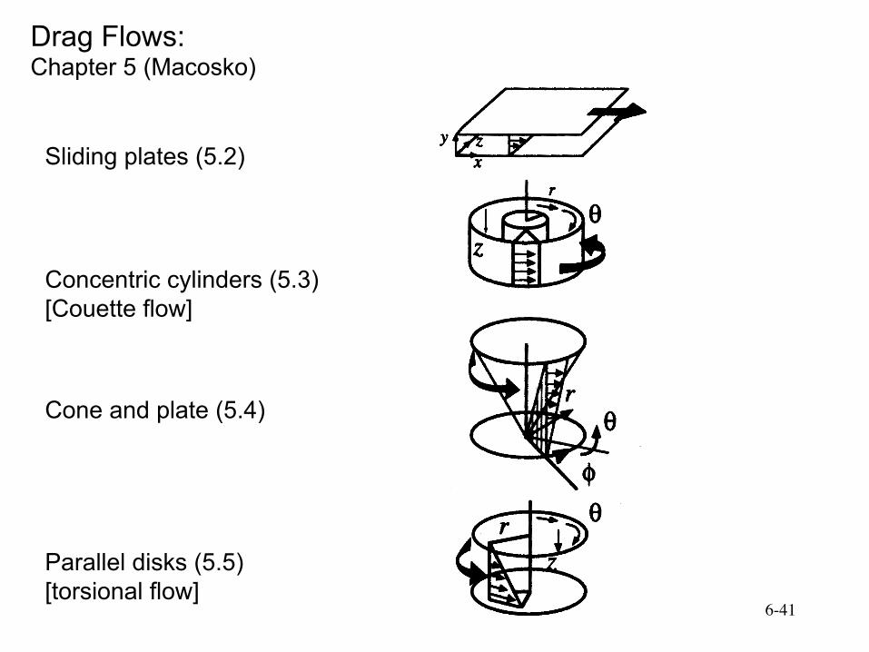
Drag Flows: Chapter 5 (Macosko)

Sliding plates (5.2)

Concentric cylinders (5.3) [Couette flow]

Cone and plate (5.4)

Parallel disks (5.5) [torsional flow]

6-42

Pressure Flows: Chapter 6 (Macosko)

Capillary (6.2) [Poiseuille flow]

Slit flow (6.3)

Axial annulus flow (6.4)

6-43

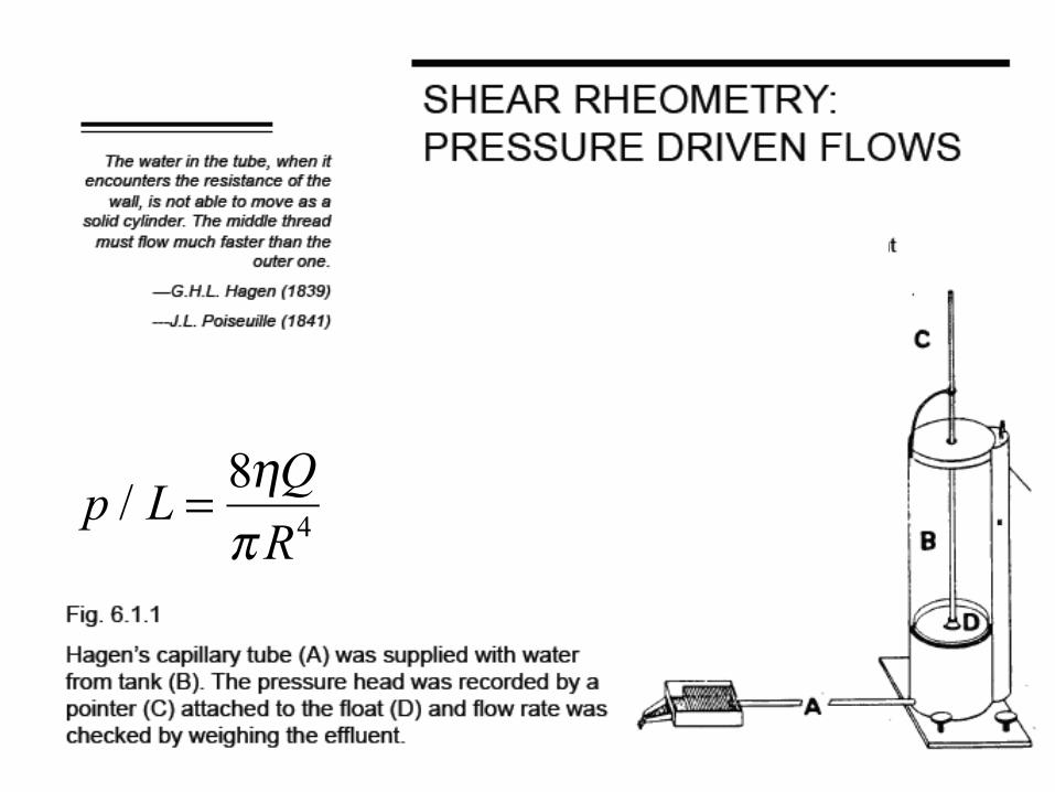
p / L = 8ηQπR4

6-44

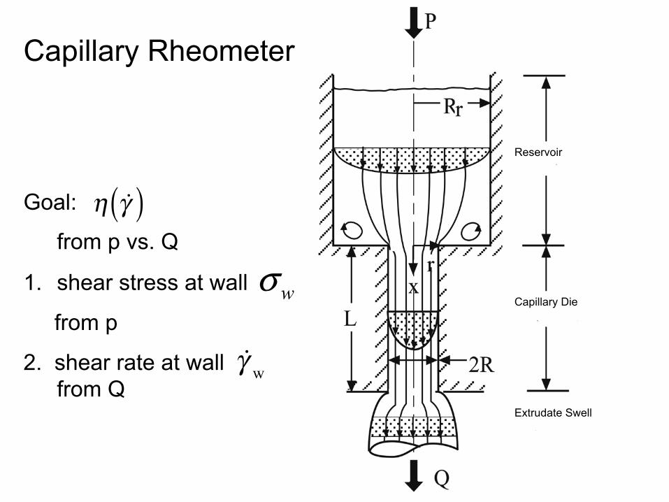
Capillary Rheometer

Reservoir

Capillary Die

Extrudate Swell

Goal:

from p vs. Q

1.  shear stress at wall

from p

2. shear rate at wall from Q

η !γ( )

!γ w

wσ

6-45

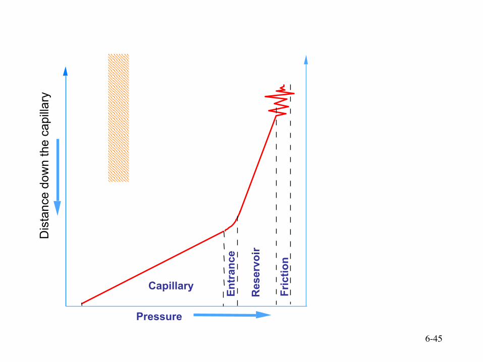
Pressure

Capillary Entr

ance

Res

ervo

ir

Fric

tion

Dis

tanc

e do

wn

the

capi

llary

F

Exit

1. Shear Stress from Pressure Drop

ptot = pfrict + pres + pen + pc

Need pc to get true shear stress

2c

wR pL

σ =

6-46

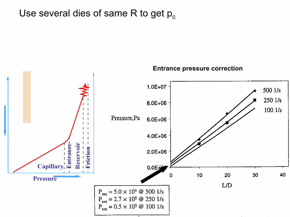
Use several dies of same R to get pc

Entrance pressure correction

Pressure Capillary E

ntra

nce

Res

ervo

ir

Fric

tion

F

Exi

t

2c

wR pL

σ =

PS 200ºC

D=1.4mm

6-47

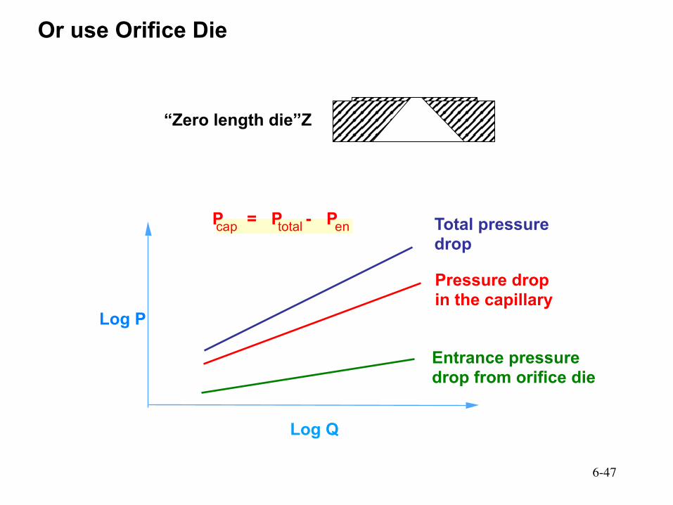
“Zero length die”Z

c a p total e n P = P - P

L o g P

L o g Q

Total pressure drop

Entrance pressure drop from orifice die

Pressure drop in the capillary

Or use Orifice Die

6-48

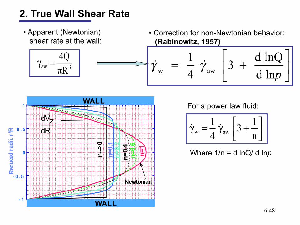
2. True Wall Shear Rate

3aw R4Q π

=γ!

!γ w = 1

4 !γ aw 3 + d lnQ

d lnp⎡

⎣⎢⎤

⎦⎥

⎥⎦⎤

⎢⎣⎡ +γ=γ

n1 3

41 aww !!

•  Apparent (Newtonian) shear rate at the wall:

•  Correction for non-Newtonian behavior: (Rabinowitz, 1957)

Where 1/n = d lnQ/ d lnp

- 1

- 0 . 5

0

0 . 5

1

R e d u

c e d r a

d i i , r / R

W A L L

W A L L

N e w t o n i a n

n = 0 . 6

n =

0 . 4

n = 1

n = 0 . 1

n =

0 . 2

n - - > 0

d V z d R

For a power law fluid:

6-49

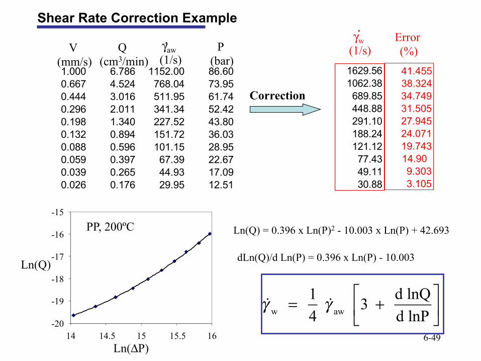
Shear Rate Correction Example

V (mm/s)

Q (cm3/min)

γaw (1/s)

P (bar)

1.000 6.786 1152.00 86.600.667 4.524 768.04 73.950.444 3.016 511.95 61.740.296 2.011 341.34 52.420.198 1.340 227.52 43.800.132 0.894 151.72 36.030.088 0.596 101.15 28.950.059 0.397 67.39 22.670.039 0.265 44.93 17.090.026 0.176 29.95 12.51

Ln(Q) = 0.396 x Ln(P)2 - 10.003 x Ln(P) + 42.693

dLn(Q)/d Ln(P) = 0.396 x Ln(P) - 10.003

!γ w = 1

4 !γ aw 3 + d lnQ

d lnP⎡

⎣⎢⎤

⎦⎥-20

-19

-18

-17

-16

-15

14 14.5 15 15.5 16

Ln(Q)

Ln(ΔP)

1629.561062.38689.85448.88291.10188.24121.1277.4349.1130.88

γw (1/s)

•

•

PP, 200ºC

Correction

41.455 38.324 34.749 31.505 27.945 24.071 19.743 14.90 9.303 3.105

Error (%)

6-50

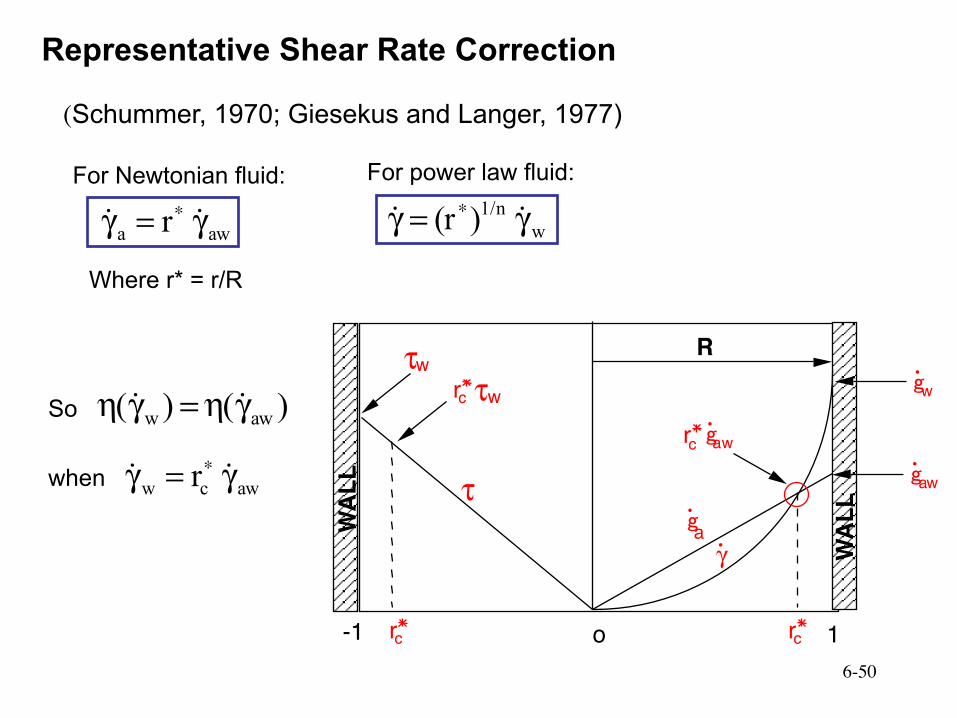
Representative Shear Rate Correction

(Schummer, 1970; Giesekus and Langer, 1977)

w1/n )(r γ=γ ∗ !!awa r γ=γ ∗ !!

For Newtonian fluid: For power law fluid:

R

- 1 o 1

γ • g • a

g • a w r c

r c r c

g • a w

g • w

W A L

L

W A L

L r c τ w

τ w

τ

So )( )( aww γη=γη !!

awcw r γ=γ ∗ !!when

Where r* = r/R

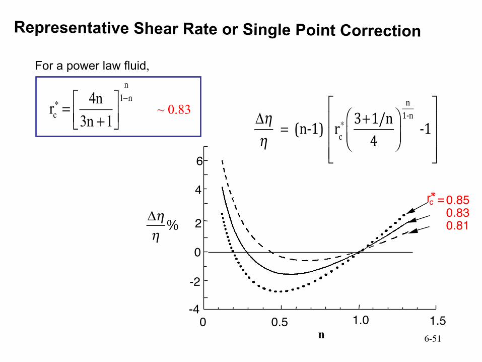
6-51

n1n

c 13n4n r

−∗⎥⎦⎤

⎢⎣⎡

+= ~ 0.83

For a power law fluid,

0 . 5

0 . 8 5 0 . 8 3 0 . 8 1

1 . 5 1 . 0 0 - 4

- 2

0

2

4

6

r c =

!

Δηη! = !(n$1)! rc∗

3+1/n4

⎛⎝⎜

⎞⎠⎟

n1$n!$1

⎡

⎣

⎢⎢⎢

⎤

⎦

⎥⎥⎥

n

Representative Shear Rate or Single Point Correction

!Δηη%

6-52

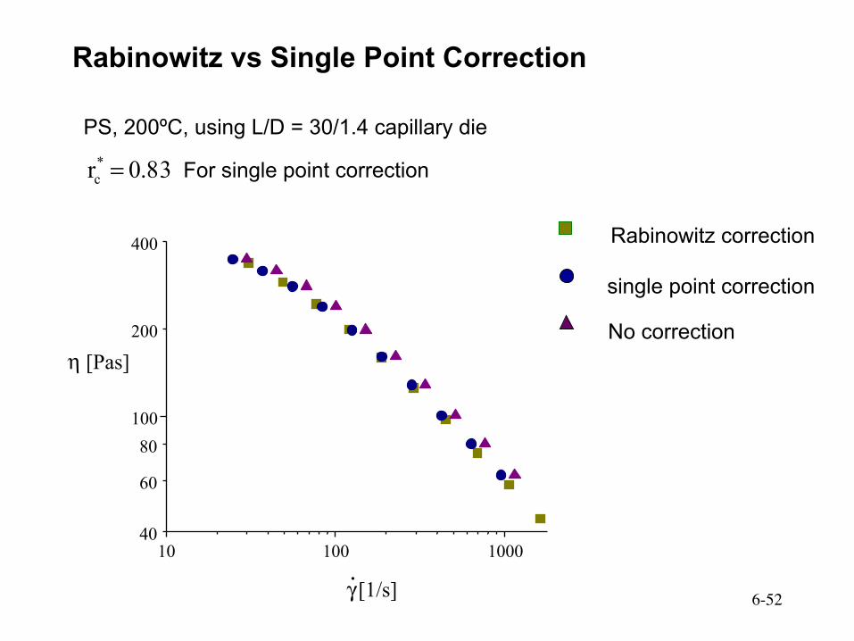
Rabinowitz vs Single Point Correction

PS, 200ºC, using L/D = 30/1.4 capillary die

0.83 r*c = For single point correction

10 100 1000 40

60

80 100

200

400 Rabinowitz correction

single point correction

No correction

γ [1/s]

η [Pas]

•

6-53

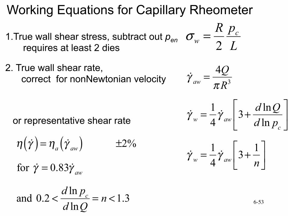
1.True wall shear stress, subtract out pen

requires at least 2 dies

Working Equations for Capillary Rheometer

2c

wR pL

σ =

2. True wall shear rate, correct for nonNewtonian velocity

!γ aw = 4QπR3

!γ w = 14!γ aw 3+ d lnQ

d ln pc

⎡

⎣⎢

⎤

⎦⎥

!γ w = 14!γ aw 3+ 1

n⎡

⎣⎢

⎤

⎦⎥

or representative shear rate

η !γ( ) =ηa !γ aw( ) ±2%

for !γ = 0.83 !γ aw

and 0.2 <d ln pc

d lnQ= n <1.3

6-54

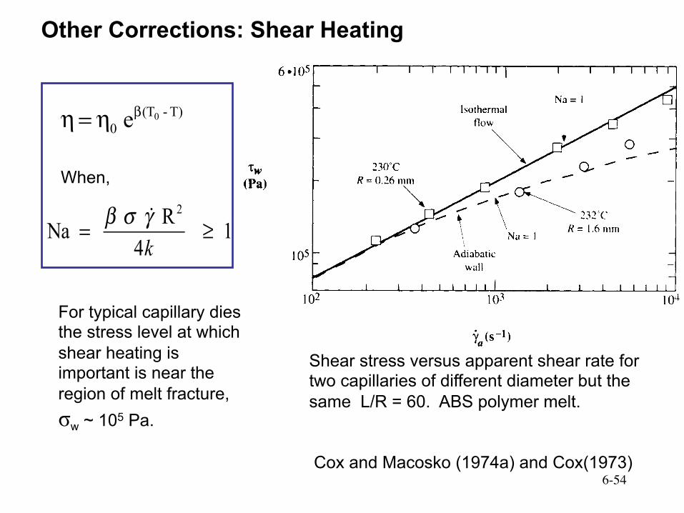
Other Corrections: Shear Heating

Na = β σ !γ R2

4k ≥ 1

T) - (T0

0e βη=η

When,

For typical capillary dies the stress level at which shear heating is important is near the region of melt fracture, σw ~ 105 Pa.

Shear stress versus apparent shear rate for two capillaries of different diameter but the same L/R = 60. ABS polymer melt. Cox and Macosko (1974a) and Cox(1973)

6-55

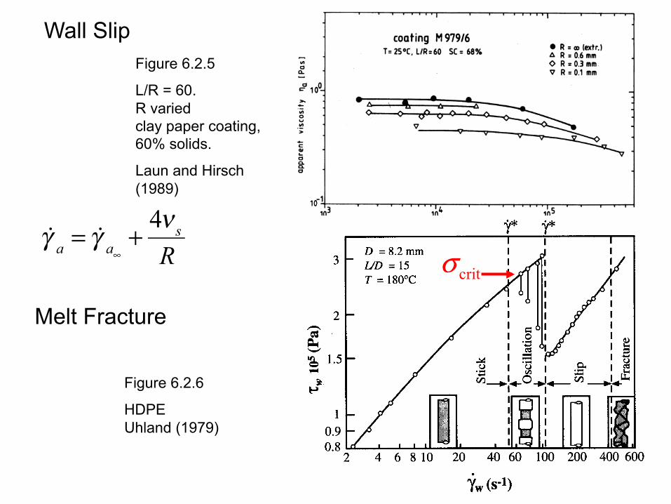
Wall Slip

Melt Fracture

!γ a = !γ a∞

+4ν s

R

Figure 6.2.6

HDPE Uhland (1979)

Figure 6.2.5

L/R = 60. R varied clay paper coating, 60% solids.

Laun and Hirsch (1989)

crit σ

6-56

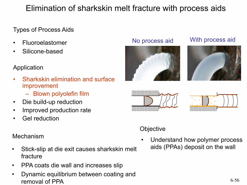
Elimination of sharkskin melt fracture with process aids

•  Fluoroelastomer •  Silicone-based

Types of Process Aids

Application

•  Sharkskin elimination and surface improvement –  Blown polyolefin film

•  Die build-up reduction •  Improved production rate •  Gel reduction

No process aid With process aid

Mechanism

•  Stick-slip at die exit causes sharkskin melt fracture

•  PPA coats die wall and increases slip •  Dynamic equilibrium between coating and

removal of PPA

Objective

•  Understand how polymer process aids (PPAs) deposit on the wall

6-57

CAPILLARY EXTRUDATE D D e

Die swell • unconstrained recovery after shear • important in extrusion operation

Assumptions:

•  isothermal, incompressible flow •  no inertial or gravity effects •  long dies, L/D>20 (i.e. no entrance effects) •  stress drops instantaneously to zero at exit •  subtract off Newtonian swell

(De/D)N = 1.13 for Re < 2

B = De/D -0.13

First normal stress difference:

First normal stress difference Coefficient:

2 2 61 wN 8 ( B -1 )σ=

21

1N γ

=ψ!

Additional Rheology via Capillary 1st Normal stress difference from extrudate swell

6-586-58

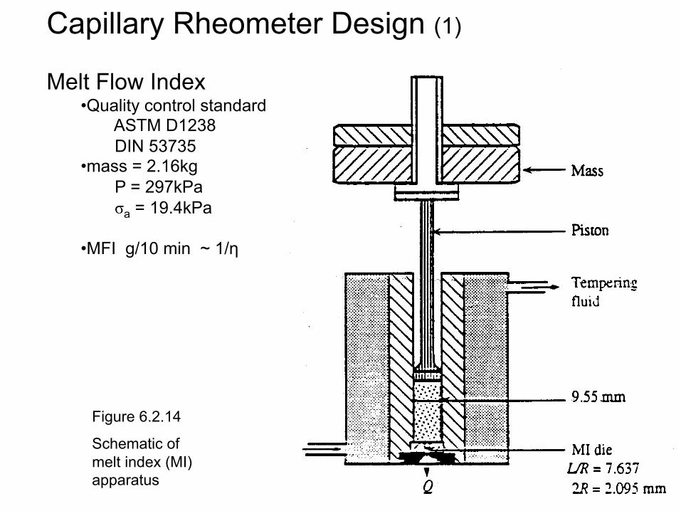
Capillary Rheometer Design (1) Melt Flow Index

• Quality control standard ASTM D1238 DIN 53735

• mass = 2.16kg P = 297kPa σa = 19.4kPa

• MFI g/10 min ~ 1/η

Figure 6.2.14

Schematic of melt index (MI) apparatus

6-59

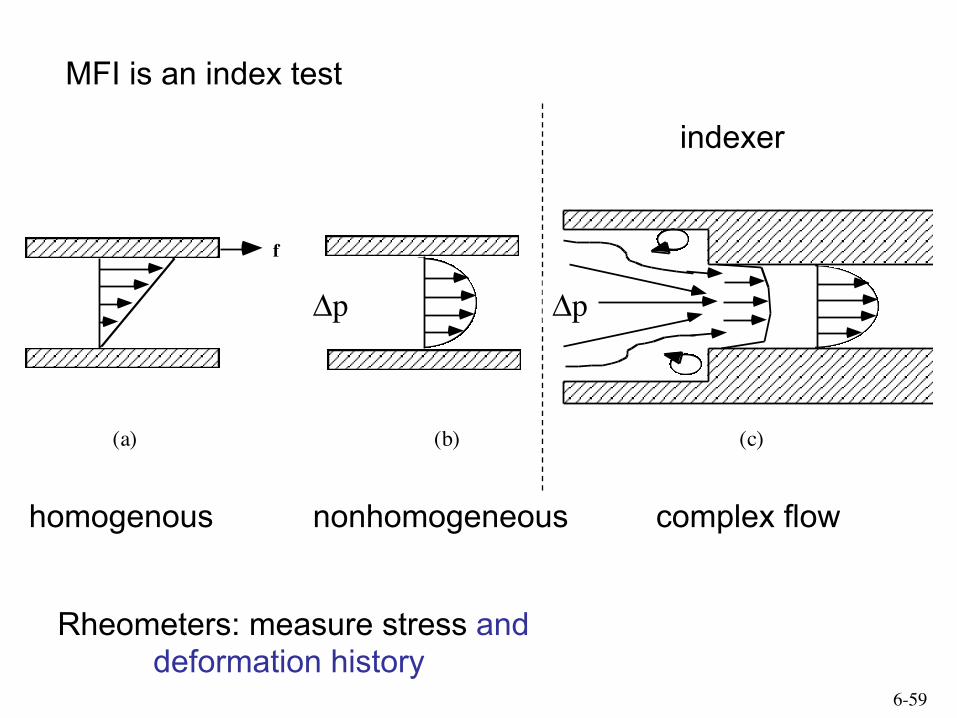
Rheometers: measure stress and deformation history

indexer

homogenous complex flow nonhomogeneous

f

p p

(a) (b) (c)

Δp Δp

MFI is an index test

6-606-60

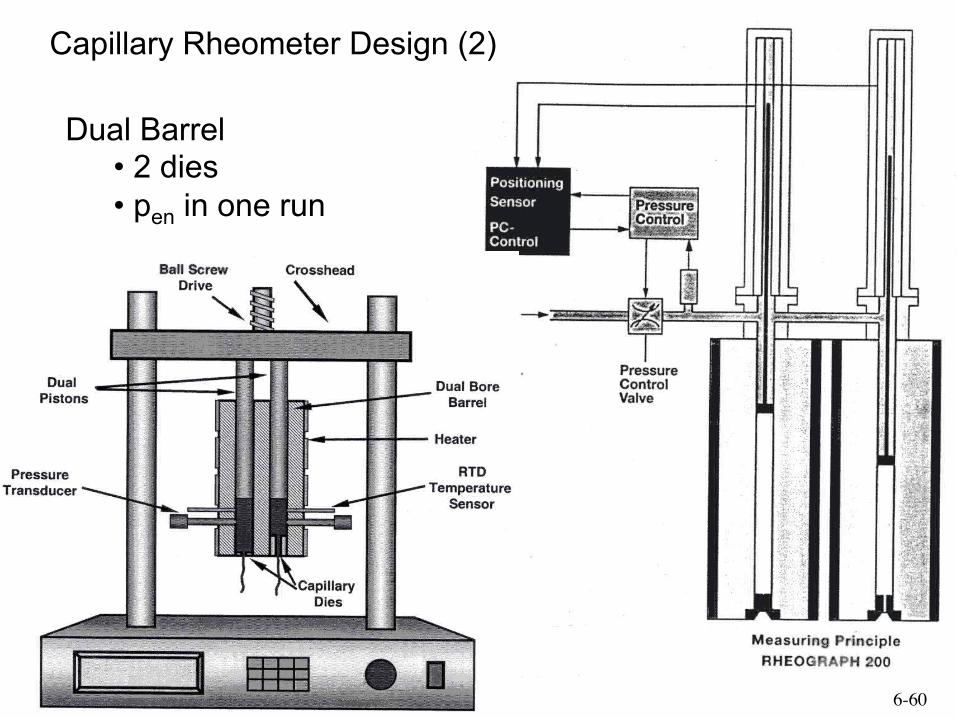
Dual Barrel •  2 dies •  pen in one run

Capillary Rheometer Design (2)

6-61

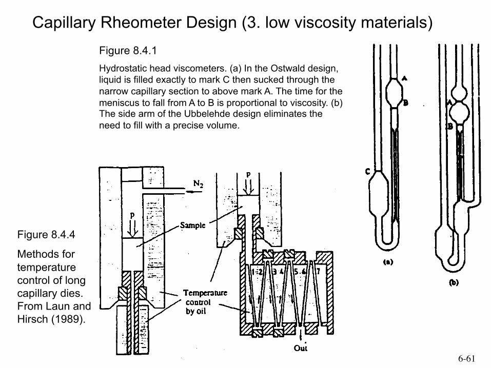
Capillary Rheometer Design (3. low viscosity materials)

Figure 8.4.4

Methods for temperature control of long capillary dies. From Laun and Hirsch (1989).

Figure 8.4.1 Hydrostatic head viscometers. (a) In the Ostwald design, liquid is filled exactly to mark C then sucked through the narrow capillary section to above mark A. The time for the meniscus to fall from A to B is proportional to viscosity. (b) The side arm of the Ubbelehde design eliminates the need to fill with a precise volume.

6-62

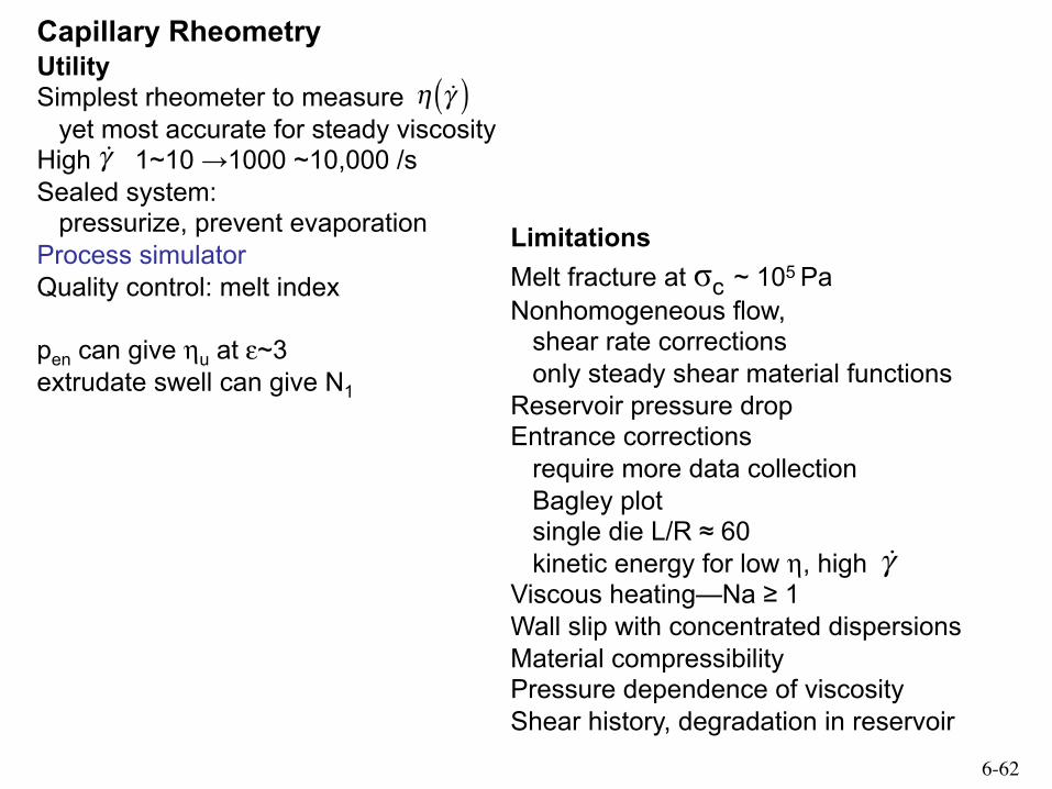
Utility Simplest rheometer to measure yet most accurate for steady viscosity High 1~10 →1000 ~10,000 /s Sealed system: pressurize, prevent evaporation Process simulator Quality control: melt index pen can give ηu at ε~3 extrudate swell can give N1

Capillary Rheometry

!γ

Limitations Melt fracture at σc ~ 105 Pa Nonhomogeneous flow, shear rate corrections only steady shear material functions Reservoir pressure drop Entrance corrections require more data collection Bagley plot single die L/R ≈ 60 kinetic energy for low η, high Viscous heating—Na ≥ 1 Wall slip with concentrated dispersions Material compressibility Pressure dependence of viscosity Shear history, degradation in reservoir

!γ

η !γ( )

6-63

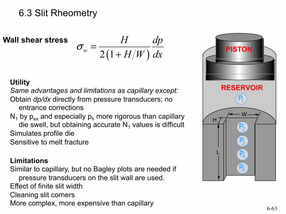
6.3 Slit Rheometry

Wall shear stress

( )2 1wH dpH W dx

σ =+

Utility Same advantages and limitations as capillary except: Obtain dp/dx directly from pressure transducers; no

entrance corrections N1 by pex and especially ph more rigorous than capillary

die swell, but obtaining accurate N1 values is difficult Simulates profile die Sensitive to melt fracture

Limitations Similar to capillary, but no Bagley plots are needed if

pressure transducers on the slit wall are used. Effect of finite slit width Cleaning slit corners More complex, more expensive than capillary

RESERVOIR

PISTON

P 2 P 3 P 4 P 5

P 1 W

H

L

6-64

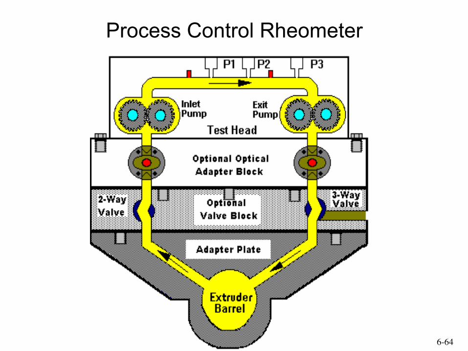
Process Control Rheometer