Sharing Equality is LinearAndrea Condoluci

Department of Computer Science and

Engineering

University of Bologna

Italy

andrea.condoluci@unibo.it

Beniamino Accaoli

LIX

Inria & Ecole Polytechnique

France

beniamino.accaoli@inria.fr

Claudio Sacerdoti Coen

Department of Computer Science and

Engineering

University of Bologna

Italy

claudio.sacerdoticoen@unibo.it

ABSTRACTe λ-calculus is a handy formalism to specify the evaluation of

higher-order programs. It is not very handy, however, when one

interprets the specication as an execution mechanism, because

terms can grow exponentially with the number of β-steps. is is

why implementations of functional languages and proof assistants

always rely on some form of sharing of subterms.

ese frameworks however do not only evaluate λ-terms, they

also have to compare them for equality. In presence of sharing, one

is actually interested in equality of the underlying unshared λ-terms.

e literature contains algorithms for such a sharing equality, that

are polynomial in the sizes of the shared terms.

is paper improves the bounds in the literature by presenting

the rst linear time algorithm. As others before us, we are inspired

by Paterson and Wegman’s algorithm for rst-order unication, it-

self based on representing terms with sharing as DAGs, and sharing

equality as bisimulation of DAGs. Beyond the improved complexity,

a distinguishing point of our work is a dissection of the involved

concepts. In particular, we show that the algorithm computes the

smallest bisimulation between the given DAGs, if any.

KEYWORDSlambda-calculus, sharing, alpha-equivalence, bisimulation

ACM Reference format:Andrea Condoluci, Beniamino Accaoli, and Claudio Sacerdoti Coen. 2016.

Sharing Equality is Linear. In Proceedings of ACM Conference, Washington,

DC, USA, July 2017 (Conference’17), 25 pages.

DOI: 10.1145/nnnnnnn.nnnnnnn

1 INTRODUCTIONOrigin and Downfall of the ProblemFor as strange as it may sound, the λ-calculus is not a good seing

for evaluating and representing higher-order programs. It is an

excellent specication framework, but—it is simply a maer of

fact—no tool based on the λ-calculus implements it as it is.

Permission to make digital or hard copies of all or part of this work for personal or

classroom use is granted without fee provided that copies are not made or distributed

for prot or commercial advantage and that copies bear this notice and the full citation

on the rst page. Copyrights for components of this work owned by others than ACM

must be honored. Abstracting with credit is permied. To copy otherwise, or republish,

to post on servers or to redistribute to lists, requires prior specic permission and/or a

fee. Request permissions from permissions@acm.org.

Conference’17, Washington, DC, USA

© 2016 ACM. 978-x-xxxx-xxxx-x/YY/MM. . .$15.00

DOI: 10.1145/nnnnnnn.nnnnnnn

Reasonable evaluation and sharing. Fix a dialect λX of the λ-

calculus with a deterministic evaluation strategy →X , and note

nfX (t) the normal form of t with respect to→X . If the λ-calculus

were a reasonable execution model then one would at least expect

that mechanizing an evaluation sequence t →nX nfX (t) on random

access machines (RAM) would have a cost polynomial in the size of

t and in the number n of β-steps. In this way a program of λX eval-

uating in a polynomial number of steps can indeed be considered

as having polynomial cost.

Unfortunately, this is not the case, at least not literally. e prob-

lem is called size explosion: there are families of terms whose size

grows exponentially with the number of evaluation steps, obtained

by nesting duplications one inside the other—simply writing down

the result nfX (t) may then require cost exponential in n.

In many cases sharing is the cure because size explosion is caused

by an unnecessary duplications of subterms, that can be avoided

if such subterms are instead shared, and evaluation is modied

accordingly.

e idea is to introduce an intermediate seing λshX where λXis rened with sharing (we are vague about sharing on purpose)

and evaluation in λX is simulated by some renement→shX of

→X . A term with sharing t represents the ordinary term t

ob-

tained by unfolding the sharing in t—the key point is that t can

be exponentially smaller than t

. Evaluation in λshX produces a

shared normal form nfshX (t) that is a compact representation of

the ordinary result, that is, such that nfshX (t)

= nfX (t

). e

situation can then be rened as in the following diagram:

λX RAM

λshX

polynomial

polynomial polynomial

Let us explain it. One says that λX is reasonably implementable if

both the simulation of λX in λshX up to sharing and the mecha-

nization of λshX can be done in time polynomial in the size of the

initial term t and of the number n of β-steps. If λX is reasonably

implementable then it is possible to reason about it as if it were not

suering of size explosion. e main consequence of such a schema

is that the number of β-steps in λX then becomes a reasonable

complexity measure—essentially the complexity class P dened in

λX coincides with the one dened by RAM or Turing machines.

e rst result in this area appeared only in the nineties and

for a special case—Blelloch and Greiner showed that weak (that

is, not under abstraction) call-by-value evaluation is reasonably

implementable [10]. e strong case, where reduction is allowed

everywhere, has received a positive answer only in 2014, when Ac-

caoli and Dal Lago have shown that lemost-outermost evaluation

is reasonably implementable [6].

arX

iv:1

907.

0610

1v1

[cs

.LO

] 1

3 Ju

l 201

9

Conference’17, July 2017, Washington, DC, USA Condoluci, Accaoli and Sacerdoti Coen

Reasonable conversion and sharing. Some higher-order seings

need more than evaluation of a single term. ey oen also have to

check whether two terms t and s are X -convertible—for instance to

implement the equality predicate, as in OCaml, or for type checking

in seings using dependent types, typically in Coq. ese frame-

works usually rely on a set of folklore and ad-hoc heuristics for

conversion, that quickly solve many frequent special cases. In the

general case, however, the only known algorithm is to rst evaluate

t and s to their normal forms nfX (t) and nfX (s) and then check

nfX (t) and nfX (s) for equality—actually, for α-equivalence because

terms in the λ-calculus are identied up to α . One can then say

that conversion in λX is reasonable if checking nfX (t) =α nfX (s)can be done in time polynomial in the sizes of t and s and in the

number of β steps to evaluate them.

Sharing is the cure for size explosion during evaluation, but what

about conversion? Size explosion forces reasonable evaluations to

produce shared results. Equality in λX unfortunately does not

trivially reduce to equality in λshX , because a single term admits

many dierent shared representations in general. erefore, one

needs to be able to test sharing equality, that is to decide whether

t

=α s

given two shared terms t and s .For conversion to be reasonable, sharing equality has to be

testable in time polynomial in the sizes of t and s . e obvious

algorithm that extracts the unfoldings t

and s

and then checks

α-equivalence is of course too naıve, because computing the un-

folding is exponential. e tricky point therefore is that sharing

equality has to be checked without unfolding the sharing.

In these terms, the question has rst been addressed by Accaoli

and Dal Lago in [5], where they provide a quadratic algorithm for

sharing equality. Consequently, conversion is reasonable.

A closer look to the costs. Once established that strong evaluation

and conversion are both reasonable it is natural to wonder how

eciently can they be implemented. Accaoli and Sacerdoti Coen

in [3] essentially show that strong evaluation can be implemented

within a bilinear overhead, i.e. with overhead linear in the size

of the initial term and in the number of β-steps. eir technique

has then been simplied by Accaoli and Guerrieri in [4]. Both

works actually address open evaluation, which is a bit simpler than

strong evaluation—the moral however is that evaluation is bilinear.

Consequently, the size of the computed result is bilinear.

e boleneck for conversion then seemed to be Accaoli and

Dal Lago’s quadratic algorithm for sharing equality. e litera-

ture actually contains also other algorithms, studied with dierent

motivations or for slightly dierent problems, discussed among re-

lated works in the next section. None of these algorithms however

matches the complexity of evaluation.

In this paper we provide the rst algorithm for sharing equality

that is linear in the size of the shared terms, improving over the

literature. erefore, the complexity of sharing equality matches

the one of evaluation, providing a combined bilinear algorithm for

conversion, that is the real motivation behind this work.

Computing Sharing EqualitySharing as DAGs. Sharing can be added to λ-terms in dierent

forms. In this paper we adopt a graphical approach. Roughly, a

λ-term can be seen as a (sort of) directed tree whose root is the

topmost constructor and whose leaves are the (free) variables. A

λ-term with sharing is more generally a Directed Acyclic Graph

(DAG). Sharing of a subterm t is then the fact that the root node nof t has more than one parent.

is type of sharing is usually called horizontal or subterm shar-

ing, and it is essentially the same sharing as in calculi with explicit

substitution, environment-based abstract machines, or linear logic—

the details are dierent but all these approaches provide dierent

incarnations of the same notion of sharing. Other types of sharing

include so-called vertical sharing (µ, letrec), twisted sharing [11],

and sharing graphs [23]. e laer provide a much deeper form of

sharing than our DAGs, and are required by Lamping’s algorithm

for optimal reduction. To our knowledge, sharing equality for shar-

ing graphs has never been studied—it is not even known whether

it is reasonable.

Sharing equality as bisimilarity. When λ-terms with sharing are

represented as DAGs, a natural way of checking sharing equal-

ity is to test DAGs for bisimilarity. Careful here: the transition

system under study is the one given by the directed edges of the

DAG, and not the one given by β-reduction steps, as in applicative

bisimilarity—our DAGs may have β-redexes but we do not reduce

them in this paper, that is an orthogonal issue, namely evaluation.

Essentially, two DAGs represent the same unfolded λ-term if they

have the same structural paths, just collapsed dierently.

To be precise, sharing equality is based on what we call shar-

ing equivalences, that are bisimulations plus some additional re-

quirements about free variables and the requirement that they are

equivalence relations.

Binders, cycles, and domination. A key point of our problem is

the presence of binders, i.e. abstractions, and the fact that equality

on usual λ-terms is α-equivalence. Graphically, it is standard to

see abstractions as geing a backward edge from the variable they

bind—a way of representing scopes that dates back to Bourbaki in

Elements de eorie des Ensembles, but also supported by the strong

relationship between λ-calculus and linear logic proof nets.

In this approach, binders introduce a form of cycle in the λ-

graph: while two free variables are bisimilar only if they coincide,

two bound variables are bisimilar only when also their binders

are bisimilar, suggesting that λ-terms with sharing are, as directed

graphs, structurally closer to deterministic nite automata (DFA),

that may have cycles, than to DAGs. e problem with cycles is

that in general bisimilarity of DAGs cannot be checked in linear

time—Hopcro and Karp’s algorithm [22], the best one, is only

pseudo-linear, that is, with an inverse Ackermann factor.

Technically speaking, the cycles induced by binders are not ac-

tual cycles: unlike usual downward edges, backwards edges do

not point to subterms of a node, but are merely a graphical repre-

sentation of scopes. ey are indeed characterized by a structural

property called domination—exploring the DAG from the root, one

necessarily visits the binder before the bound variable. Domination

turns out to be one of the key ingredients for a linear algorithm in

presence of binders.

Previous work. Sharing equality bears similarities with unica-

tion, which are discussed in the next section. For what concerns

Sharing Equality is Linear Conference’17, July 2017, Washington, DC, USA

sharing equality itself, in the literature there are only two algo-

rithms explicitly addressing it. First, the already cited quadratic

one by Accaoli and Dal Lago. Second, a O(n logn) algorithm by

Grabmayer and Rochel [21] (where n is the sum of the sizes of the

shared terms to compare, and the input of the algorithm is a graph),

obtained by a reduction to equivalence of DFAs and treating the

more general case of λ-terms with letrec.

Contributions: a theory and a 2-levels linear algorithm. is paper

is divided in two parts. e rst part develops a re-usable, self-

contained, and clean theory of sharing equality, independent of

the algorithm that computes it. Some of its concepts are implicitly

used by other authors, but never emerged from the collective un-

conscious before (propagated queries in particular)—others instead

are new. A key point is that we bypass the use of α-equivalence

by relating sharing equalities on DAGs with λ-terms represented

in a locally nameless way [17]. In such an approach, bound names

are represented using de Bruijn indices, while free variables are

represented using names—thus α-equivalence collapses on equality.

e theory culminates with the sharing equality theorem, which

connects equality of λ-terms and sharing equivalences on shared

λ-terms, under suitable conditions.

e second part studies a linear algorithm for sharing equality

by adapting Paterson and Wegman’s (shortened to PW) linear algo-

rithm for rst-order unication [27] to λ-terms with sharing. Our

algorithm is actually composed by a 2-levels, modular approach,

pushing further the modularity suggested—but not implemented—

in the nominal unication study by Calves & Fernandez in [15]:

• Blind check: a reformulation of PW from which we re-

moved the management of meta-variables for unication.

It is used as a rst-order test on λ-terms with sharing, to

check that the unfolded terms have the same skeleton,

ignoring variables.

• Variables check: a straightforward algorithm executed aer

the previous one, testing α-equivalence by checking that

bisimilar bound variables have bisimilar binders and that

two dierent free variables are never equated.

e decomposition plus the correctness and the completeness of

the checks crucially rely on the theory developed in the rst part.

e value of the paper. It is delicate to explain the value of our

work. ree contributions are clear: 1) the improved complexity

of the problem, 2) the consequent downfall on the complexity of

β-conversion, and 3) the isolation of a theory of sharing equality. At

the same time, however, our algorithm looks as an easy adaptation

of PW, and binders do not seem to play much of a role. Let us then

draw aention to the following points:

• Identication of the problem: the literature presents similar

studies and techniques, and yet we are the rst to formulate

and study the problem per se (unication is dierent, and it

is usually not formulated on terms with sharing), directly

(i.e. without reducing it to DFAs, like in Grabmayer and

Rochel), and with a ne-grained look at the complexity

(Accaoli and Dal Lago only tried not to be exponential).

• e role of binders: the fact that binders can be treated

straightforwardly is—we believe—an insight and not a

weakness of our work. Essentially, domination allows to

reduce sharing equality in presence of binders to the Blind

check, under key assumptions on the context in which

terms are tested (see queries, Sect. 4).

• Minimality. e set of shared representations of an ordi-

nary λ-term t is a laice: the boom element is t itself, the

top element is the (always existing) maximally sharing of t ,and for any two terms with sharing there exist inf and sup.

Essentially, Accaoli & Dal Lago and Grabmayer & Rochel

address sharing equality by computing the top elements of

the laices of the two λ-terms with sharing, and then com-

paring them for α-equivalence. We show that our Blind

check—and morally every PW-based algorithm—computes

the sup of t and s , that is, the term having all and only the

sharing in t or s , that is the smallest sharing equivalence

between the two DAGs. is insight, rst pointed out in

PW’s original paper to characterize most general uniers,

is a prominent concept in our theory of sharing equality

as well.

• Proofs, invariants, and detailed development. We provide de-

tailed correctness, completeness, and linearity proofs, plus

a detailed treatment of the relationship between equality

on locally nameless λ-terms and sharing equivalences on

λ-graphs. Our work is therefore self-contained, but for the

fact that most of the theorems and their proofs have been

moved to the appendix.

• Concrete implementation. We implemented our algorithm

1and veried experimentally its linear time complexity.

However, let us stress that despite providing an imple-

mentation our aim is mainly theoretical. Namely, we are

interested in showing that sharing equality is linear (to ob-

tain that conversion is bilinear) and not only pseudo-linear,

even though other algorithms with super-linear asymptotic

complexity may perform beer in practice.

2 RELATED PROBLEMS AND TECHNICALCHOICES

We suggest the reader to skip this section at a rst reading.

Related problems. ere are various problems that are closely re-

lated to sharing equality, and that are also treated with bisimilarity-

based algorithms. Let us list similarities and dierences:

• First-order unication. On the one hand the problem is more

general, because unication roughly allows to substitute

variables with terms not present in the original DAGs,

while in sharing equality this is not possible. On the other

hand, the problem is less general, because it does not allow

binders and does not testα-equivalence. ere are basically

two linear algorithm for rst-order unication, Paterson

and Wegman’s (PW) [27] and Martelli and Montanari’s

(MM) [26]. Both rely on sharing to be linear. PW even takes

terms with sharing as inputs, while MM deals with sharing

in a less direct way, except in its less known variant [25]

that takes in input terms shared using the Boyer-Moore

technique [12].

1e code is available on hp://www.cs.unibo.it/∼sacerdot/sharing equivalence.tgz.

Conference’17, July 2017, Washington, DC, USA Condoluci, Accaoli and Sacerdoti Coen

• Nominal unication is unication up to α-equivalence (but

not up to β or η equivalence) of λ-calculi extended with

name swapping, in the nominal tradition. It has rst stud-

ied by Urban, Pis, and Gabbay [31] and ecient algo-

rithms are due to two groups, Calves & Fernandez and

Levy & Villaret, adapting PW and MM form rst-order uni-

cation. It is very close to sharing equality, but the known

best algorithms [15, 24] are only quadratic. See [14] for a

unifying presentation.

• Paern unication. Miller’s paern unication can also be

stripped down to test sharing equality. Qian presents a PW-

inspired algorithm, claiming linear complexity [28], that

seems to work only on unshared terms. We say claiming

because the algorithm is very involved and the proofs are

far from being clear. Moreover, according to Levy and

Villaret in [24]: it is really dicult to obtain a practical

algorithm from the proof described in [28]. We believe that

is fair to say that Qian’s work is hermetic (please try to

read it!).

• Nominal matching. Calves & Fernandez in [16] present an

algorithm for nominal matching (a special case of unica-

tion) that is linear, but only on unshared input terms.

• Equivalence of DFA. Automata do not have binders, and

yet they are structurally more general than λ-terms with

sharing, since they allow arbitrary directed cycles, not

necessarily dominated. As already pointed out, the best

equivalence algorithm is only pseudo-linear [22].

Algorithms for α-equivalence extended with further principles (e.g.

permutations of let expressions), but not up to sharing unfolding,

is studied by Schmidt-Schauß, Rau, and Sabel in [30].

Hash-consing. Hash-consing [18, 20] is a technique to share

purely functional data, traditionally realised through a hash ta-

ble [7]. It is a eager approach to conversion of λ-terms, in which

one keeps trace in a huge table of all the pairs of convertible terms

previously encountered. Our approach is somewhat dual or lazy,

as our technique does not record previous tests, only the current

equality problem is analysed. With hash consing, to check that

two terms are sharing equivalent it suces to perform a lookup

in the hash table, but rst the terms have to be hash-consed (i.e.

maximally shared), which requires quasilinear running times.

Technical choices. Our algorithm requires λ-terms to be repre-

sented as graphs. is choice is fair, since abstract machines with

global environments such as those described by Accaoli and Bar-

ras in [2] do manipulate similar representations, and thus produce

λ-graphs to be compared for sharing equality—moreover, it is es-

sentially the same representation induced by the translation of

λ-calculus into linear logic proof nets [1, 29] up to explicit sharing

nodes—namely ?-links—and explicit boxes. In this paper we do not

consider explicit sharing nodes (that in λ-calculus syntax corre-

spond to have sharing only on variables), but one can translate in

linear time between that representation to ours (and viceversa) by

collapsing these variables-as-sharing on their child if they are the

child of some other node. Our results could be adapted to this other

approach, but at the price of more technical denitions.

On the other hand, abstract machines with local environments

(e.g. Krivine asbtract machine), that typically rely on de Bruijn

indices, produce dierent representations where every subterm is

paired with an environment, representing a delayed substitution.

ose outputs cannot be directly compared for sharing equality,

they rst have to be translated to a global environment representation—

the study of such a translation is future work.

3 PRELIMINARIESIn this section we introduce λ-graphs, the representation of λ-terms

with sharing that we consider in this paper. First of all we introduce

the usual λ-calculus without sharing.

λ-terms and equality. e syntax of λ-terms is usually dened as

follows:

(Named) Terms t , s ::= x | λx .t | t sis representation of λ-terms is called named, since variables and

abstractions bear names. Equality on named terms is not just syntac-

tic equality, but α-equality: terms are identied up to the renaming

of bound variables, because for example the named terms λx .λy.xand λy.λx .y should denote the same λ-term.

is is the standard representation of λ-terms, but reasoning

in presence of names is cumbersome, especially names for bound

variables as they force the introduction of α-equivalence classes.

Moreover nodes naturally bear no names, thus we prefer to avoid

assigning arbitrary variable names when performing the readback

of a node to a λ-term.

On closed λ-terms (terms with only bound variables), this sug-

gests a nameless approach: by using de Bruijn indices, variables

simply consist of an index, a natural number indicating the number

of abstractions that occur between the abstraction to which the

variable is bound and that variable occurrence. For example, the

named term λx .λy.x and the nameless term λλ1 denote the same λ-

term. e nameless representation can be extended to open λ-terms,

but it adds complications because for example dierent occurrences

of the same free variable unnaturally have dierent indices.

Since we are forced to work with open terms (because proof as-

sistants require them) the most comfortable representation and the

one we adopt in our proofs is the locally nameless representation

(see Chargueraud [17] for a thorough discussion). is represen-

tation combines named and nameless, by using de Bruijn indices

for bound variables (thus avoiding the need for α-equivalence),

and names for free variables. is representation of λ-terms is

the most faithful to our denition of λ-graphs: as we shall see, to

compare two bound variable nodes one compares their binders,

but to compare two free variable nodes one uses their identier,

which in implementations is usually their memory address or a

user-supplied string.

e syntax of locally nameless (l.n.) terms is:

(l.n.) Terms t , s ::= i | a | t s | λt (i ∈ N, a ∈ A)where i denotes a bound variable of de Bruijn index i (N is the set

of natural numbers), and a denotes a free variable of name a (A is

a set of atoms).

In the rest of the paper, we switch seamlessly between dierent

representations of λ-terms (without sharing): we use named terms

in examples, as they are more human-friendly, but locally nameless

Sharing Equality is Linear Conference’17, July 2017, Washington, DC, USA

a)@

|| ##λ

@

@

λ

x

::

λ

##

y

77

y

88

w

b)@

λ

@

@

x

II

λ

y

77

w

c)@

λ

@

x

GG

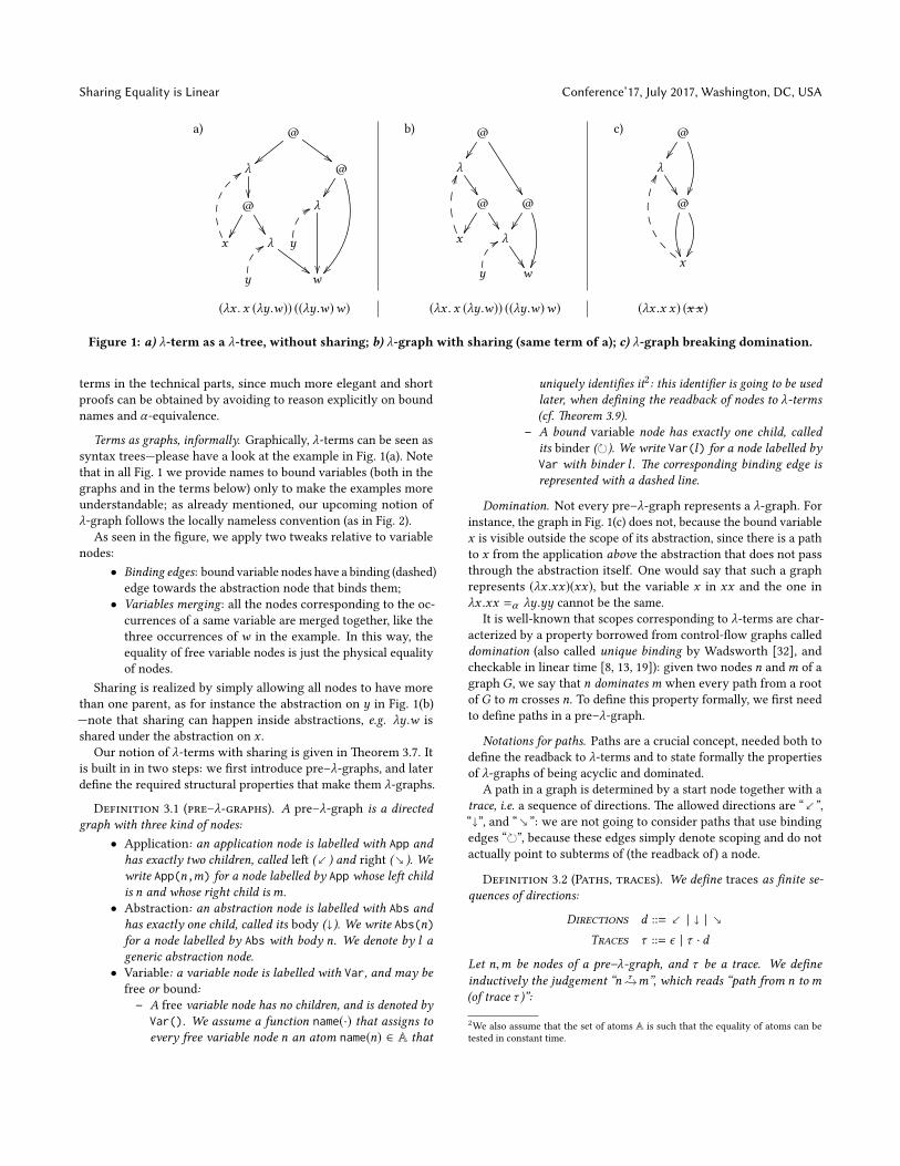
(λx . x (λy.w)) ((λy.w)w) (λx . x (λy.w)) ((λy.w)w) (λx .x x) (x x)

Figure 1: a) λ-term as a λ-tree, without sharing; b) λ-graph with sharing (same term of a); c) λ-graph breaking domination.

terms in the technical parts, since much more elegant and short

proofs can be obtained by avoiding to reason explicitly on bound

names and α-equivalence.

Terms as graphs, informally. Graphically, λ-terms can be seen as

syntax trees—please have a look at the example in Fig. 1(a). Note

that in all Fig. 1 we provide names to bound variables (both in the

graphs and in the terms below) only to make the examples more

understandable; as already mentioned, our upcoming notion of

λ-graph follows the locally nameless convention (as in Fig. 2).

As seen in the gure, we apply two tweaks relative to variable

nodes:

• Binding edges: bound variable nodes have a binding (dashed)

edge towards the abstraction node that binds them;

• Variables merging: all the nodes corresponding to the oc-

currences of a same variable are merged together, like the

three occurrences of w in the example. In this way, the

equality of free variable nodes is just the physical equality

of nodes.

Sharing is realized by simply allowing all nodes to have more

than one parent, as for instance the abstraction on y in Fig. 1(b)

—note that sharing can happen inside abstractions, e.g. λy.w is

shared under the abstraction on x .

Our notion of λ-terms with sharing is given in eorem 3.7. It

is built in in two steps: we rst introduce pre–λ-graphs, and later

dene the required structural properties that make them λ-graphs.

Definition 3.1 (pre–λ-graphs). A pre–λ-graph is a directed

graph with three kind of nodes:

• Application: an application node is labelled with App and

has exactly two children, called le (

) and right (

). We

write App(n,m) for a node labelled by App whose le child

is n and whose right child ism.

• Abstraction: an abstraction node is labelled with Abs and

has exactly one child, called its body (

). We write Abs(n)for a node labelled by Abs with body n. We denote by l a

generic abstraction node.

• Variable: a variable node is labelled with Var, and may be

free or bound:

– A free variable node has no children, and is denoted by

Var(). We assume a function name(·) that assigns to

every free variable node n an atom name(n) ∈ A that

uniquely identies it2: this identier is going to be used

later, when dening the readback of nodes to λ-terms

(cf. eorem 3.9).

– A bound variable node has exactly one child, called

its binder (). We write Var(l) for a node labelled by

Var with binder l . e corresponding binding edge is

represented with a dashed line.

Domination. Not every pre–λ-graph represents a λ-graph. For

instance, the graph in Fig. 1(c) does not, because the bound variable

x is visible outside the scope of its abstraction, since there is a path

to x from the application above the abstraction that does not pass

through the abstraction itself. One would say that such a graph

represents (λx .xx)(xx), but the variable x in xx and the one in

λx .xx =α λy.yy cannot be the same.

It is well-known that scopes corresponding to λ-terms are char-

acterized by a property borrowed from control-ow graphs called

domination (also called unique binding by Wadsworth [32], and

checkable in linear time [8, 13, 19]): given two nodes n andm of a

graph G, we say that n dominates m when every path from a root

of G to m crosses n. To dene this property formally, we rst need

to dene paths in a pre–λ-graph.

Notations for paths. Paths are a crucial concept, needed both to

dene the readback to λ-terms and to state formally the properties

of λ-graphs of being acyclic and dominated.

A path in a graph is determined by a start node together with a

trace, i.e. a sequence of directions. e allowed directions are “

”,

“

”, and “

”: we are not going to consider paths that use binding

edges “”, because these edges simply denote scoping and do not

actually point to subterms of (the readback of) a node.

Definition 3.2 (Paths, traces). We dene traces as nite se-

quences of directions:

Directions d ::=| |

Traces τ ::= ϵ | τ · d

Let n,m be nodes of a pre–λ-graph, and τ be a trace. We dene

inductively the judgement “n τ m”, which reads “path from n to m(of trace τ )”:

2We also assume that the set of atoms A is such that the equality of atoms can be

tested in constant time.

Conference’17, July 2017, Washington, DC, USA Condoluci, Accaoli and Sacerdoti Coen

a)@

@

@

@

@

λ

λ

λ

λ

v

FF

v

EE

v

EE

v

EE

b)@

@

λ

v

EE

c) λ

λ

v

GG

v

GG d) λ

λ

v

GG

v

GG e) λ

λ

v

GG

v

GG

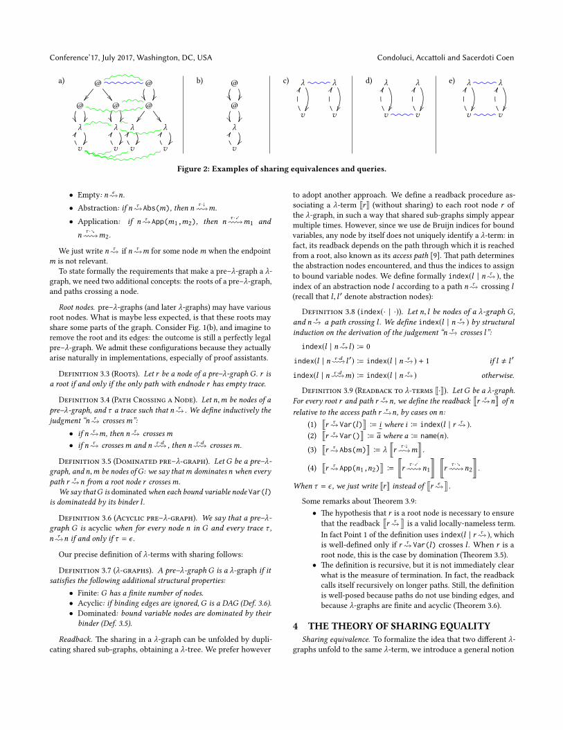
Figure 2: Examples of sharing equivalences and queries.

• Empty: n ϵ n.

• Abstraction: if n τ Abs(m), then nτ ·

m.

• Application: if n τ App(m1,m2), then nτ ·

m1 and

nτ ·

m2.

We just write n τif n τ m for some nodem when the endpoint

m is not relevant.

To state formally the requirements that make a pre–λ-graph a λ-

graph, we need two additional concepts: the roots of a pre–λ-graph,

and paths crossing a node.

Root nodes. pre–λ-graphs (and later λ-graphs) may have various

root nodes. What is maybe less expected, is that these roots may

share some parts of the graph. Consider Fig. 1(b), and imagine to

remove the root and its edges: the outcome is still a perfectly legal

pre–λ-graph. We admit these congurations because they actually

arise naturally in implementations, especially of proof assistants.

Definition 3.3 (Roots). Let r be a node of a pre–λ-graph G . r is

a root if and only if the only path with endnode r has empty trace.

Definition 3.4 (Path Crossing a Node). Let n,m be nodes of a

pre–λ-graph, and τ a trace such that n τ. We dene inductively the

judgment “n τcrossesm”:

• if n τ m, then n τcrossesm

• if n τcrossesm and n τ ·d

, then n τ ·dcrossesm.

Definition 3.5 (Dominated pre–λ-graph). Let G be a pre–λ-

graph, and n,m be nodes ofG : we say thatm dominates n when every

path r τ n from a root node r crossesm.

We say thatG is dominated when each bound variable node Var(l)is dominatedd by its binder l .

Definition 3.6 (Acyclic pre–λ-graph). We say that a pre–λ-

graph G is acyclic when for every node n in G and every trace τ ,

n τ n if and only if τ = ϵ .

Our precise denition of λ-terms with sharing follows:

Definition 3.7 (λ-graphs). A pre–λ-graph G is a λ-graph if it

satises the following additional structural properties:

• Finite: G has a nite number of nodes.

• Acyclic: if binding edges are ignored, G is a DAG (Def. 3.6).

• Dominated: bound variable nodes are dominated by their

binder (Def. 3.5).

Readback. e sharing in a λ-graph can be unfolded by dupli-

cating shared sub-graphs, obtaining a λ-tree. We prefer however

to adopt another approach. We dene a readback procedure as-

sociating a λ-term JrK (without sharing) to each root node r of

the λ-graph, in such a way that shared sub-graphs simply appear

multiple times. However, since we use de Bruijn indices for bound

variables, any node by itself does not uniquely identify a λ-term: in

fact, its readback depends on the path through which it is reached

from a root, also known as its access path [9]. at path determines

the abstraction nodes encountered, and thus the indices to assign

to bound variable nodes. We dene formally index(l | n τ ), the

index of an abstraction node l according to a path n τcrossing l

(recall that l , l ′ denote abstraction nodes):

Definition 3.8 (index(· | ·)). Let n, l be nodes of a λ-graph G,

and n τa path crossing l . We dene index(l | n τ ) by structural

induction on the derivation of the judgement “n τcrosses l”:

index(l | n τ l) B 0

index(l | n τ ·d l ′) B index(l | n τ ) + 1 if l , l ′

index(l | n τ ·d m) B index(l | n τ ) otherwise.

Definition 3.9 (Readback to λ-terms J·K). Let G be a λ-graph.

For every root r and path r τ n, we dene the readback

qr τ n

yof n

relative to the access path r τ n, by cases on n:

(1)

qr τ Var(l)

yB i where i B index(l | r τ ).

(2)

qr τ Var()

yB a where a B name(n).

(3)

qr τ Abs(m)

yB λ

rr

τ ·

mz

.

(4)

qr τ App(n1,n2)

yB

sr

τ ·

n1

sr

τ ·n2

.

When τ = ϵ , we just write JrK instead of

qr ϵ

y.

Some remarks about eorem 3.9:

• e hypothesis that r is a root node is necessary to ensure

that the readback

qr τ

yis a valid locally-nameless term.

In fact Point 1 of the denition uses index(l | r τ ), which

is well-dened only if r τ Var(l) crosses l . When r is a

root node, this is the case by domination (eorem 3.5).

• e denition is recursive, but it is not immediately clear

what is the measure of termination. In fact, the readback

calls itself recursively on longer paths. Still, the denition

is well-posed because paths do not use binding edges, and

because λ-graphs are nite and acyclic (eorem 3.6).

4 THE THEORY OF SHARING EQUALITYSharing equivalence. To formalize the idea that two dierent λ-

graphs unfold to the same λ-term, we introduce a general notion

Sharing Equality is Linear Conference’17, July 2017, Washington, DC, USA

•n R n

n R m

m R n

n R m m R p

n R p

App(n1,n2) R App(m1,m2) n1 R m1

App(n1,n2) R App(m1,m2) n2 R m2

Abs(n) R Abs(m)

n R m

Var(n) R Var(m)

n R m

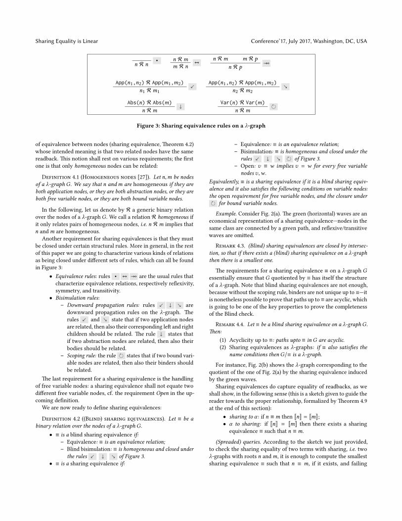
Figure 3: Sharing equivalence rules on a λ-graph

of equivalence between nodes (sharing equivalence, eorem 4.2)

whose intended meaning is that two related nodes have the same

readback. is notion shall rest on various requirements; the rst

one is that only homogeneous nodes can be related:

Definition 4.1 (Homogeneous nodes [27]). Let n,m be nodes

of a λ-graph G. We say that n and m are homogeneous if they are

both application nodes, or they are both abstraction nodes, or they are

both free variable nodes, or they are both bound variable nodes.

In the following, let us denote by R a generic binary relation

over the nodes of a λ-graph G . We call a relation R homogeneous if

it only relates pairs of homogeneous nodes, i.e. n R m implies that

n andm are homogeneous.

Another requirement for sharing equivalences is that they must

be closed under certain structural rules. More in general, in the rest

of this paper we are going to characterize various kinds of relations

as being closed under dierent sets of rules, which can all be found

in Figure 3:

• Equivalence rules: rules • are the usual rules that

characterize equivalence relations, respectively reexivity,

symmetry, and transitivity.

• Bisimulation rules:

– Downward propagation rules: rules

are

downward propagation rules on the λ-graph. e

rules

and

state that if two application nodes

are related, then also their corresponding le and right

children should be related. e rule

states that

if two abstraction nodes are related, then also their

bodies should be related.

– Scoping rule: the rule states that if two bound vari-

able nodes are related, then also their binders should

be related.

e last requirement for a sharing equivalence is the handling

of free variable nodes: a sharing equivalence shall not equate two

dierent free variable nodes, cf. the requirement Open in the up-

coming denition.

We are now ready to dene sharing equivalences:

Definition 4.2 ((Blind) sharing eqivalences). Let ≡ be a

binary relation over the nodes of a λ-graph G.

• ≡ is a blind sharing equivalence if:

– Equivalence: ≡ is an equivalence relation;

– Blind bisimulation: ≡ is homogeneous and closed under

the rules

of Figure 3.

• ≡ is a sharing equivalence if:

– Equivalence: ≡ is an equivalence relation;

– Bisimulation: ≡ is homogeneous and closed under the

rules

of Figure 3.

– Open: v ≡ w implies v = w for every free variable

nodes v,w .

Equivalently, ≡ is a sharing equivalence if it is a blind sharing equiv-

alence and it also satises the following conditions on variable nodes:

the open requirement for free variable nodes, and the closure under

for bound variable nodes.

Example. Consider Fig. 2(a). e green (horizontal) waves are an

economical representation of a sharing equivalence—nodes in the

same class are connected by a green path, and reexive/transitive

waves are omied.

Remark 4.3. (Blind) sharing equivalences are closed by intersec-

tion, so that if there exists a (blind) sharing equivalence on a λ-graph

then there is a smallest one.

e requirements for a sharing equivalence ≡ on a λ-graph Gessentially ensure that G quotiented by ≡ has itself the structure

of a λ-graph. Note that blind sharing equivalences are not enough,

because without the scoping rule, binders are not unique up to ≡—it

is nonetheless possible to prove that paths up to≡ are acyclic, which

is going to be one of the key properties to prove the completeness

of the Blind check.

Remark 4.4. Let ≡ be a blind sharing equivalence on a λ-graphG .

en:

(1) Acyclicity up to ≡: paths upto ≡ in G are acyclic.

(2) Sharing equivalences as λ-graphs: if ≡ also satises the

name conditions then G/≡ is a λ-graph.

For instance, Fig. 2(b) shows the λ-graph corresponding to the

quotient of the one of Fig. 2(a) by the sharing equivalence induced

by the green waves.

Sharing equivalences do capture equality of readbacks, as we

shall show, in the following sense (this is a sketch given to guide the

reader towards the proper relationship, formalized by eorem 4.9

at the end of this section):

• sharing to α : if n ≡m then JnK = JmK;• α to sharing: if JnK = JmK then there exists a sharing

equivalence ≡ such that n ≡m.

(Spreaded) queries. According to the sketch we just provided,

to check the sharing equality of two terms with sharing, i.e. two

λ-graphs with roots n andm, it is enough to compute the smallest

sharing equivalence ≡ such that n ≡ m, if it exists, and failing

Conference’17, July 2017, Washington, DC, USA Condoluci, Accaoli and Sacerdoti Coen

otherwise. is is what our algorithm does. At the same time,

however, it is slightly more general: it may test more than two

nodes at the same time, i.e. all the pairs of nodes contained in a

query.

Definition 4.5 (ery). A query Q over a λ-graphG is a binary

relation over the root nodes of G.

e simplest case is when there are only two roots n and mand the query contains only n Q m (depicted as a blue wave in

Fig. 2(a))—from now on however we work with a generic query Q,

which may relate nodes that are roots of not necessarily disjoint

or even distinct λ-graphs; our focus is on the smallest sharing

equivalence containing Q.

Let us be more precise. Every query Q induces a number of

other equality requests obtained by closing Q with respect to the

equivalence and propagation clauses that every sharing equivalence

has to satisfy. In other words, every query induces a spreaded query.

Definition 4.6 (Spreading R#). Let R be a binary relation over

the nodes of a λ-graphG . e spreadingR#induced byR is the binary

relation on the nodes of G inductively dened by closing R under the

rules •

of Figure 3.

Example. e spreading Q#of the (blue) query Q in Fig. 2(a) is

the (reexive and transitive closure) of the green waves.

Blind universality of Q#. Note that the spreaded query Q#

is de-

ned without knowing if there exists a (blind) sharing equivalence

containing the queryQ—there might very well be none (if the nodes

are not sharing equivalent). It turns out that the spreaded query

Q#is itself a blind sharing equivalence, whenever there exists a

blind sharing equivalence containing the query Q. In that case,

unsurprisingly, Q#is also the smallest blind sharing equivalence

containing the query Q.

Proposition 4.7 (Blind universality of Q#). Let Q be a query.

If there exists a blind sharing equivalence ≡ containing Q then:

(1) e spreaded query Q#is contained in ≡, i.e. Q# ⊆ ≡.

(2) Q#is the smallest blind sharing equivalence containing Q.

Cycles up to Q#. Let us apply eorem 4.4(1) to Q#

, and take

the contrapositive statement: if paths up to Q#are cyclic then

Q#is not a blind sharing equivalence. e Blind Check in Sect. 6

indeed fails as soon as it nds a cycle up to Q#. Note, now, that

Q#satises the equivalence and bisimulation requirements for a

blind sharing equivalence by denition. e only way in which it

might not be such an equivalence then, is if it is not homogeneous.

Said dierently, there is in principle no need to check for cycles, it

is enough to test for homogeneity. We are going to do it anyway,

because cycles provide earlier failures—there are also other practical

reasons to do so, to be discussed in Sect. 6.

Universality of the spreaded query Q#. Here it lies the key con-

ceptual point in extending the linearity of Paterson and Wegman’s

algorithm to binders and working up to α-equivalence of bound

variables.

In general the spreading R#of a binary relation R may not be a

sharing equivalence, even though a sharing equivalence containing

R exists. Consider for instance the relation R in Fig. 2(d): R coin-

cides with its spreadingR#(up to reexivity), which is not a sharing

equivalence because it does not include the Abs-nodes above the

original query—note that spreading only happens downwards. To

obtain a sharing equivalence one has to also include the Abs-nodes

(Fig. 2(e)). e example does not show it, but in general then one has

to start over spreading the new relation (eventually having to add

other Abs-nodes found in the process, and so on). ese iterations

are obviously problematic in order to keep linear the complexity of

the procedure—a key point of Paterson and Wegman’s algorithm is

that every node is processed only once.

What makes possible to extend their algorithm to binders is that

the query is context-free, i.e. it is not in the scope of any abstraction,

which is the case since it involves only pairs of roots, that therefore

are above all abstractions as in Fig. 2(c). en—remarkably—there

is no need to iterate the propagation of the query. Said dierently,

if the relation Q is context-free then Q#is universal.

e structural property of λ-graphs guaranteeing the absence of

iterations for context-free queries is domination. Domination asks

that to reach a bound variable from outside its scope one necessarily

needs to rst pass through its binder. e intuition is that if one

starts with a context-free query then there is no need to iterate

because binders are necessarily visited before the variables while

propagating the query downwards.

Let us stress, however, that it is not evident that domination

is enough. In fact, domination is about one bound variable and

its only binder. For sharing equivalence instead one deals with a

class of equivalent variables and a class of binders—said dierently,

domination is given in a seing without queries, and is not obvious

that it gets along well with them. e fact that domination on single

binders is enough for spreaded queries to be universal requires

indeed a non-trivial proof and it is a somewhat surprising fact.

Proposition 4.8 (Universality of Q#). Let Q be a query over a

λ-graph G . If there exists a sharing equivalence ≡ containing Q, then

the spreaded query Q#is the smallest sharing equivalence containing

Q.

e proof of this proposition is in Appendix A.4, page 17, where

it is obtained as a corollary of other results connecting equality of

λ-terms and sharing equivalences, that also rely crucially on the

the fact that queries only relate roots. It can also be proved directly,

but it requires a very similar reasoning, which is why we rather

prove it indirectly.

e sharing equality theorem. We have now introduced all the

needed concepts to state the precise connection between the equal-

ity of λ-terms, queries, and sharing equivalences, which is the main

result of our abstract study of sharing equality.

Theorem 4.9 (Sharing eqality). Let Q be a query over a λ-

graph G. Q#is a sharing equivalence if and only if JnK = JmK for

every nodes n,m such that n Q m.

Despite the—we hope—quite intuitive nature of the theorem, its

proof is delicate and requires a number of further concepts and

lemmas, developed in Appendices A–B. e key point is nding

an invariant expressing how queries on roots propagate under

abstractions and interact with domination, until they eventually

satisfy the name conditions for a sharing equivalence, and vice

versa.

Sharing Equality is Linear Conference’17, July 2017, Washington, DC, USA

Let us conclude the section by stressing a subtlety of eorem 4.9.

Consider Fig. 2(c)—with that query the statement is satised. Con-

sider Fig. 2(d)—that relation is not a valid query because it does not

relate root nodes, and in fact the statement would fail because the

readback of the two queried nodes are not the same and not even

well-dened. Consider the relation R in Fig. 2(e)—now R and R#

coincide (up to reexivity) and R#is a sharing equivalence, but the

theorem (correctly) fails, because not all queried pairs of nodes are

equivalent, as in Fig. 2(d).

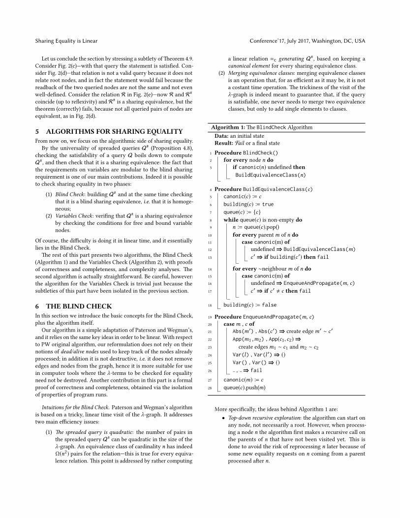
5 ALGORITHMS FOR SHARING EQUALITYFrom now on, we focus on the algorithmic side of sharing equality.

By the universality of spreaded queries Q#(Proposition 4.8),

checking the satisfability of a query Q boils down to compute

Q#, and then check that it is a sharing equivalence: the fact that

the requirements on variables are modular to the blind sharing

requirement is one of our main contributions. Indeed it is possible

to check sharing equality in two phases:

(1) Blind Check: building Q#and at the same time checking

that it is a blind sharing equivalence, i.e. that it is homoge-

neous;

(2) Variables Check: vering that Q#is a sharing equivalence

by checking the conditions for free and bound variable

nodes.

Of course, the diculty is doing it in linear time, and it essentially

lies in the Blind Check.

e rest of this part presents two algorithms, the Blind Check

(Algorithm 1) and the Variables Check (Algorithm 2), with proofs

of correctness and completeness, and complexity analyses. e

second algorithm is actually straightforward. Be careful, however:

the algorithm for the Variables Check is trivial just because the

subtleties of this part have been isolated in the previous section.

6 THE BLIND CHECKIn this section we introduce the basic concepts for the Blind Check,

plus the algorithm itself.

Our algorithm is a simple adaptation of Paterson and Wegman’s,

and it relies on the same key ideas in order to be linear. With respect

to PW original algorithm, our reformulation does not rely on their

notions of dead/alive nodes used to keep track of the nodes already

processed; in addition it is not destructive, i.e. it does not remove

edges and nodes from the graph, hence it is more suitable for use

in computer tools where the λ-terms to be checked for equality

need not be destroyed. Another contribution in this part is a formal

proof of correctness and completeness, obtained via the isolation

of properties of program runs.

Intuitions for the Blind Check. Paterson and Wegman’s algorithm

is based on a tricky, linear time visit of the λ-graph. It addresses

two main eciency issues:

(1) e spreaded query is quadratic: the number of pairs in

the spreaded query Q#can be quadratic in the size of the

λ-graph. An equivalence class of cardinality n has indeed

Ω(n2) pairs for the relation—this is true for every equiva-

lence relation. is point is addressed by rather computing

a linear relation =c generating Q#, based on keeping a

canonical element for every sharing equivalence class.

(2) Merging equivalence classes: merging equivalence classes

is an operation that, for as ecient as it may be, it is not

a costant time operation. e trickiness of the visit of the

λ-graph is indeed meant to guarantee that, if the query

is satisable, one never needs to merge two equivalence

classes, but only to add single elements to classes.

Algorithm 1: e BlindCheck Algorithm

Data: an initial state

Result: Fail or a nal state

1 Procedure BlindCheck()2 for every node n do3 if canonic(n) undened then

BuildEquivalenceClass(n)

4 Procedure BuildEquivalenceClass(c)5 canonic(c) B c

6 building(c) B true

7 queue(c) B c8 while queue(c) is non-empty do9 n B queue(c).pop()

10 for every parentm of n do11 case canonic(m) of12 undened ⇒ BuildEquivalenceClass(m)

13 c ′⇒ if building(c ′) then fail

14 for every ∼neighbourm of n do15 case canonic(m) of16 undened ⇒ EnqueueAndPropagate(m, c)

17 c ′⇒ if c ′ , c then fail

18 building(c) B false

19 Procedure EnqueueAndPropagate(m, c)20 casem , c of21 Abs(m′) , Abs(c ′)⇒ create edgem′ ∼ c ′22 App(m1,m2) , App(c1, c2)⇒23 create edgesm1 ∼ c1 andm2 ∼ c2

24 Var(l) , Var(l ′) ⇒ ()25 Var() , Var() ⇒ ()26 , ⇒ fail

27 canonic(m) B c

28 queue(c).push(m)

More specically, the ideas behind Algorithm 1 are:

• Top-down recursive exploration: the algorithm can start on

any node, not necessarily a root. However, when process-

ing a node n the algorithm rst makes a recursive call on

the parents of n that have not been visited yet. is is

done to avoid the risk of reprocessing n later because of

some new equality requests on n coming from a parent

processed aer n.

Conference’17, July 2017, Washington, DC, USA Condoluci, Accaoli and Sacerdoti Coen

• ery edges: the query is represented through additional

undirected query edges between nodes, and it is propagated

on child nodes by adding further query edges. e query

is propagated carefully, on-demand. e fully propagated

query is never computed, because, as explained, in general

its size is quadratic in the number of nodes.

• Canonic edges: when a node is visited, it is assigned a

canonic node that is a representative of its sharing equiva-

lence class. is is represented via a directed canonic edge,

which is implemented as a pointer.

• Building ag: each node has a boolean “building” ag that

is used only by canonic representatives and notes the state

of construction of their equivalence class. When unde-

ned, it means that that node is not currently designated

as canonic; when true, it means that the equivalence class

of that canonic is still being computed; when false, it signals

that the equivalence class has been completely computed.

• Failures and cycles: the algorithm fails in three cases. First,

when it nds two nodes in the same class that are not homo-

geneous (Line 26), because then the approximation of Q#

that it is computing cannot be a blind sharing equivalence.

e two other cases (on Line 13 and Line 17) the algorithm

uses the fact that the canonic edge is already present to

infer that it found a cycle up to Q#, and so, again Q#

can-

not be a blind sharing equivalence (please read again the

paragraph aer Proposition 4.7).

• Building a class: calling BuildEquivalenceClass(n) boils

down to

(1) collect without duplicates all the nodes in the intended

sharing equivalence class of n, that is, the nodes re-

lated ton by a sequence of query edges. is is done by

the while loop at Line 14, that rst collects the nodes

queried with n and then iterates on the nodes queried

with them. ese nodes are inserted in a queue;

(2) setn as the canonical element of its class, by seing the

canonical edge of every node in the class (including

n) to n;

(3) propagate the query on the children (in case n is a Lamor a App node), by adding query edges between the

corresponding children of every node in the class and

their canonic.

(4) Pushing a node in the queue, seing its canonic, and

propagating the query on its children is done by the

procedure EnqueueAndPropagate.

• Linearity: let us now come back to the two eciency issues

we mentioned before:

– Merging classes: the recursive calls are done in order to

guarantee that when a node is processed all the query

edges for its sharing class are already available, so

that the class shall not be extended nor merged with

other classes later on during the visit of the λ-graph.

– Propagating the query: the query is propagated only

aer having set the canonics of the current sharing

equivalence class. To explain, consider a class of knodes, which in general can be dened by Ω(k2) query

edges. Note that aer canonization, the class is rep-

resented using only k − 1 canonic edges, and thus

the algorithm propagates onlyO(k) query edges—this

is why the number of query edges is kept linear in

the number of the nodes (assuming that the original

query itself was linear). If instead one would propa-

gate query edges before canonizing the class, then the

number of query edges may grow quadratically.

States. As explained, the algorithm needs to enrich λ-graphs

with a few additional concepts, namely canonic edges, query edges,

building ags, queues, and execution stack, all grouped under the

notion of program state.

A state S of the algorithm is either Fail or a tuple

(G, undir, canonic, building, queue, active)

where G is a λ-graph, and the remaining data structures have the

following properties:

• Undirected query edges (∼): undir is a multiset of undi-

rected query edges, pairing nodes that are expected to be

placed by the algorithm in the same sharing equivalence

class. Undirected loops are admied and there may be

multiple occurrences of an undirected edge between two

nodes. More precisely, for every undirected edge between

n and m with multiplicty k in the state, both (n,m) and

(m,n) belong with multiplicity k to undir. We denote by

∼ the binary relation over G such that n ∼m i the edge

(n,m) belongs to undir.

• Canonic edges (c): nodes may have one additional canonicdirected edge pointing to the computed canonical repre-

sentative of that node. e partial function mapping each

node to its canonical representative (if dened) is noted

c. We then write c(n) =m if the canonical of n is m, and

c(n) = undefined otherwise. By abuse of notation, we

also consider c a binary relation on G, where n c m i

c(n) =m.

• Building ags (b): nodes may have an additional boolean

ag building that signals whether an equivalence class

has or has not been constructed yet. e partial function

mapping each node to its building ag (if dened) is noted

b. We then write b(n) = true | false if the building ag

of n is dened, and b(n) = undefined otherwise.

• eues (q): nodes have a queue data structure that is used

only on canonic representatives, and contains the nodes of

the class that are going to be processed next. e partial

function mapping each node to its queue (if dened) is

noted q.

• Active Calls (active): a program state contains informa-

tion on the execution stack of the algorithm, including the

active procedures, local variables, and current execution

line. We leave the concept of execution stack informal;

we only dene more formally active, which records the

order of visit of equivalence classes that are under con-

struction, and that is essential in the proof of complete-

ness of the algorithm. active is an abstraction of the

implicit execution stack of active calls to the procedure

Sharing Equality is Linear Conference’17, July 2017, Washington, DC, USA

BuildEquivalenceClass where only (part of) the acti-

vation frames for BuildEquivalenceClass(c) are repre-

sented. Formally, active is simply a sequence of nodes of

the λ-graph, and active = [c1, . . . , cK ] if and only if:

– Active: BuildEquivalenceClass(c1), . . . ,

BuildEquivalenceClass(cK) are exactly the

calls to BuildEquivalenceClass that are currently

active, i.e. have been called before S, but have not yet

returned;

– Call Order: for every 0 < i < j ≤ K ,

BuildEquivalenceClass(ci) was called before

BuildEquivalenceClass(c j).

Moreover we introduce the following concepts:

• Program transition: the change of state caused by the execu-

tion of a piece of code. For the sake of readability, we avoid

a technical denition of transitions; roughly, a transition is

the execution of a line of code, as they appear numbered in

the algorithm itself. When the line is a while loop, a tran-

sition is an iteration of the body, or the exit from the loop;

when the line is a if-then-else, a transition is entering

one of the branches according to the condition; and so on.

• Fail state: Fail is the state reached aer executing a failinstruction; it has no aributes and no transitions.

• Initial state S0: a non-Fail state with the following at-

tributes:

– Initial ∼edges: simply the initial query, i.e. ∼ B Q.

– Initial assignments: c(n), b(n), and q(n) are undened

for every node n of G.

– Initial transition: the rst transition is a call to

BlindCheck().

• Program run: a sequence of program states starting from

S0 obtained by consecutive transitions.

• Reachable: a state which is the last state of a program run.

• Failing: a reachable state that transitions to Fail.

• Final: a non-Fail reachable state that has no further transi-

tions.

Details about how the additional structures of enriched λ-graphs

are implemented are given in Sect. 6.2, where the complexity of the

algorithm is analysed.

6.1 Correctness and CompletenessHere we prove that Algorithm 1 correctly and completely solves

the blind sharing equivalence problem, that is, it checks whether

the spreaded query is a blind sharing equivalence.

e proofs rely on a number of general properties of program

runs and reachable states. e full statements and proofs are in

Appendix D, grouped according to the concepts that they analyze.

Correctness. We prove that whenever Algorithm 1 terminates

successfully with nal state Sf from an initial query Q, then Q#

is homogeneous, and therefore a blind sharing equivalence. Addi-

tionally, we show that the canonic assignment is a succint repre-

sentation of Q#, i.e. that for all nodes n,m: n Q# m if and only if

n andm have the same canonic assigned in Sf . e following are

the most important properties to prove correctness:

• Blind bisimulation upto: in all reachable states, c is a blind

bisimulation upto (∼ ∪ =).• Undirected query edges approximate the spreaded query: in

all reachable states, Q ⊆ ∼ ⊆ Q#.

• e canonic assignment respects the ∼ constraints: in all

reachable states, c ⊆ ∼∗• Eventually, all query edges are visited: in all nal states, all

query edges are subsumed by the canonic assignment, i.e.

∼ ⊆ c∗.

In every reachable state, we dene =c as the equivalence relation

over the λ-graph that equates two nodes whenever their canonic

representatives are both dened and coincide. e lemmas above

basically state that during the execution of the algorithm, =c is a

blind sharing equivalence up to the query edges, and that ∼ can

indeed be seen as an approximation of the spreaded query Q#. At

the end of the algorithm, ∼ and c actually represent the same (up

to the (·)∗ closure) relation =c, which is then exactly the spreaded

query:

Proposition 6.1 (Correctness). In every nal state Sf :

• Succint representation: (=c) = (Q#),• Blind check: Q#

is homogeneous, and therefore a blind shar-

ing equivalence.

Completeness. Completeness is the fact that whenever Algo-

rithm 1 fails, Q#is not a blind sharing equivalence. Recall that

the algorithm can fail only while executing the following three

lines of code:

• On Line 13 during BuildEquivalenceClass, when a node

n is being processed and it has a parent whose equivalence

class is still being built;

• On Line 17 during BuildEquivalenceClass, when a node

n is being processed and it has a ∼neighbour belonging to

a dierence equivalence class;

• On Line 26 during EnqueueAndPropagate(m,c), when the

algorithm is trying two relate the nodesm and c which are

not homogeneous.

While in the laer case (Line 26) the failure of the homogeneous

condition is more evident, in the rst two cases it is more subtle. In

fact, when the homogeneous condition fails on Line 13 and Line 17

it is not because we explicitly found two related nodes that are not

homogeneous, but because Q#does not satisfy an indirect property

that is necessary for Q#to be homogenous (see below). In these

cases the algorithm fails early, even though it has not visited yet

the actual pair of nodes that are not homogeneous.

To justify the early failures we use active, which basi-

cally records the equivalence classes that the algorithm is build-

ing in a given state, sorted according to the order of calls to

BuildEquivalenceClass. Nodes in active respect a certain strict

order: if active = [c1, . . . , cK ], then c1 ≺ c2 ≺ . . . ≺ cK (eo-

rem D.27 in the Appendix), where n ≺ m implies that the equiv-

alence class of n is a child of the one of m in the quotient graph.

e algorithm fails on Line 13 and Line 17 because it found a cyclic

chain of nodes related by ≺, therefore nding a cycle in the quo-

tient graph. By eorem 4.4, there cannot exist any blind sharing

equivalence containing the initial query in this case.

Conference’17, July 2017, Washington, DC, USA Condoluci, Accaoli and Sacerdoti Coen

Proposition 6.2 (Completeness). If Algorithm 1 fails, thenQ#is

not a blind sharing equivalence, and therefore by the blind universality

ofQ#(eorem 4.7), there does not exist any blind sharing equivalence

containing the initial query Q.

6.2 LinearityIn this section we show that Algorithm 1 always terminates, and

it does so in time linear in the size of the λ-graph and the initial

query.

Low-level assumptions. In order to analyse the complexity of the

algorithm we have to spell out some details about an hypothetical

implementation on a RAM of the data structures used by the Blind

check.

• Nodes: since Line 2 of the algorithm needs to iterate on all

nodes of the λ-graph, we assume an array of pointers to

all the nodes of the graph.

• Directed edges: these edges—despite being directed—have

to be traversed in both directions, typically to recurse over

the parents of a node. We then assume that every node has

an array of pointers to its parents.

• Undirected query edges: query edges are undirected and

are dynamically created; in addition, the algorithm needs

to iterate on all ∼neighbours of a node. In order to obtain

the right complexity, every node simply maintains a linked

list of its ∼neighbours, in such a way that when a new

undirected edge (n,m) is created, then n is pushed on the

list of ∼neighbours ofm, andm on the one of n.

• Canonical assignment is obtained by a pointer to a node

(possibly undefined) in the data structure for nodes.

• Building ags are just implemented via a boolean on each

node.

• eues do not need to be recorded in the data structure for

nodes, as they can be equivalently coded as local variables.

Let us call atomic the following operations performed by the

check: nding the rst node, nding the next node given the previ-

ous node, nding the rst parent of a node, nding the next parent

of a node given the previous parent, checking and seing canonics,

checking and seing building ags, geing the next query edge on

a given node, traversing a query edge, adding a query edge between

two nodes, pushing to a queue, and popping an element o of a

queue.

Lemma 6.3 (Atomic operations are constant). e atomic

operations of the Blind check are all implementable in constant time

on a RAM.

Termination and linearity of the algorithm are proved via a

global estimation of the number of transitions in a program run.

e dicult part is to estimate the number of transitions execut-

ing lines of BuildEquivalenceClass, since it contains multiple

nested loops. First of all, we prove that in every program run

BuildEquivalenceClass is called at most once for each node.

en, also the body of the while loop on Line 8 is executed in

total at most once for each node, because we prove that in a pro-

gram run each node is enqueued at most once. Since the parents of

a node do not change during a program run, the loop on Line 10

is not problematic. As for the loop on Line 14 on the ∼neighbours

of a node n, we prove that the ∼neighbours of n do not change

aer the parents of n are visited. Finally, recall that the algorithm

parsimoniously propagates query edges only between a node and

its canonic: as a consequence, in every reachable state |undir| islinear in the size of Q and the number of nodes in the λ-graph.

Let |G | denote the size of a λ-graph G, i.e. the number of nodes

and edges of G. en:

Proposition 6.4 (Linear termination). Let S0 be an initial

state of the algorithm, with a query Q over a λ-graph G. en the

Blind check terminates in a number of transitions linear in |G | and

|Q|.

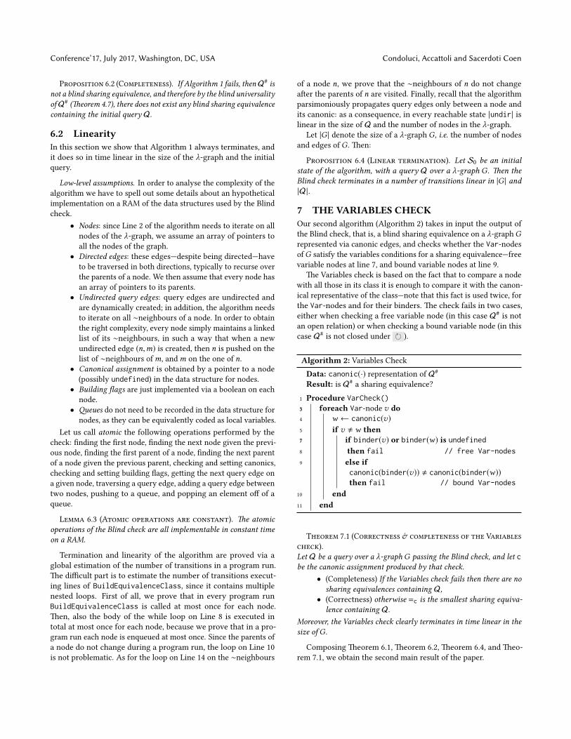
7 THE VARIABLES CHECKOur second algorithm (Algorithm 2) takes in input the output of

the Blind check, that is, a blind sharing equivalence on a λ-graphGrepresented via canonic edges, and checks whether the Var-nodes

ofG satisfy the variables conditions for a sharing equivalence—free

variable nodes at line 7, and bound variable nodes at line 9.

e Variables check is based on the fact that to compare a node

with all those in its class it is enough to compare it with the canon-

ical representative of the class—note that this fact is used twice, for

the Var-nodes and for their binders. e check fails in two cases,

either when checking a free variable node (in this case Q#is not

an open relation) or when checking a bound variable node (in this

case Q#is not closed under ).

Algorithm 2: Variables Check

Data: canonic(·) representation of Q#

Result: is Q#a sharing equivalence?

1 Procedure VarCheck()33 foreach Var-node v do4 w ← canonic(v)5 if v , w then77 if binder(v) or binder(w) is undefined8 then fail // free Var-nodes

9 else ifcanonic(binder(v)) , canonic(binder(w))then fail // bound Var-nodes

10 end11 end

Theorem 7.1 (Correctness & completeness of the Variables

check).

Let Q be a query over a λ-graph G passing the Blind check, and let cbe the canonic assignment produced by that check.

• (Completeness) If the Variables check fails then there are no

sharing equivalences containing Q,

• (Correctness) otherwise =c is the smallest sharing equiva-

lence containing Q.

Moreover, the Variables check clearly terminates in time linear in the

size of G.

Composing eorem 6.1, eorem 6.2, eorem 6.4, and eo-

rem 7.1, we obtain the second main result of the paper.

Sharing Equality is Linear Conference’17, July 2017, Washington, DC, USA

Theorem 7.2 (Sharing eqality is linear). Let Q be a query

over a λ-graph G. e sharing equality algorithm obtained by com-

bining Algorithm 1 and Algorithm 2 runs in time linear in the sizes

ofG and Q, and it succeeds if and only if there exists a sharing equiv-

alence containing Q. Moreover, if it succeeds, it outputs a concrete

(and linear) representation of the smallest such sharing equivalence.

Finally, composing with the sharing equality theorem (eo-

rem 4.9) one obtains that the algorithm indeed tests the equality of

the readbacks of the query, as expected.

8 CONCLUSIONSWe presented the rst linear-time algorithm to check the sharing

equivalence of λ-graphs. Following our development of the theory

of sharing equality, we split the algorithm in two parts: a rst part

performing a check on the DAG structure of λ-graphs, and the

second part checking the additional requirements on variables and

scopes. e paper is accompanied by a technical report with formal

proofs of correctness, completeness, and termination in linear time.

e motivation for this work stemmed from our previous works

on the evaluation of λ-terms: abstract machines can reduce a λ-

term to normal form in time bilinear in the size of the term and the

number of evaluation steps, if λ-terms are represented in memory

as λ-graphs. When combining bilinear evaluation through abstract

machines and the sharing equality algorithm presented here, one

obtains a bilinear algorithm for conversion. As a consequence,

αβ-conversion can be implemented with only bilinear overhead.

ACKNOWLEDGMENTSis work has been partially funded by the ANR JCJC grant

COCA HOLA (ANR-16-CE40-004-01) and the COST Action EU-

Types CA15123 STSM#43345.

REFERENCES[1] Beniamino Accaoli. 2018. Proof Nets and the Linear Substitution Calculus. In

eoretical Aspects of Computing - ICTAC 2018 - 15th International Colloquium,

Stellenbosch, South Africa, October 16-19, 2018, Proceedings. 37–61. hps://doi.

org/10.1007/978-3-030-02508-3 3

[2] Beniamino Accaoli and Bruno Barras. 2017. Environments and the complexity

of abstract machines. In Proceedings of the 19th International Symposium on

Principles and Practice of Declarative Programming, Namur, Belgium, October 09 -

11, 2017. 4–16. hps://doi.org/10.1145/3131851.3131855

[3] Beniamino Accaoli and Claudio Sacerdoti Coen. 2015. On the Relative Use-

fulness of Fireballs. In 30th Annual ACM/IEEE Symposium on Logic in Computer

Science, LICS 2015, Kyoto, Japan, July 6-10, 2015. 141–155. hps://doi.org/10.

1109/LICS.2015.23

[4] Beniamino Accaoli and Giulio Guerrieri. 2017. Implementing Open Call-by-

Value. In Fundamentals of Soware Engineering - 7th International Conference,

FSEN 2017, Tehran, Iran, April 26-28, 2017, Revised Selected Papers. 1–19. hps:

//doi.org/10.1007/978-3-319-68972-2 1

[5] Beniamino Accaoli and Ugo Dal Lago. 2012. On the Invariance of the Unitary

Cost Model for Head Reduction. In 23rd International Conference on Rewriting

Techniques and Applications (RTA’12) , RTA 2012, May 28 - June 2, 2012, Nagoya,

Japan. 22–37. hps://doi.org/10.4230/LIPIcs.RTA.2012.22

[6] Beniamino Accaoli and Ugo Dal Lago. 2014. Beta reduction is invariant, indeed.

In Joint Meeting of the Twenty-ird EACSL Annual Conference on Computer

Science Logic (CSL) and the Twenty-Ninth Annual ACM/IEEE Symposium on Logic

in Computer Science (LICS), CSL-LICS ’14, Vienna, Austria, July 14 - 18, 2014.

8:1–8:10. hps://doi.org/10.1145/2603088.2603105

[7] John Allen. 1978. Anatomy of LISP. McGraw-Hill, Inc., New York, NY, USA.

[8] Stephen Alstrup, Dov Harel, Peter W. Lauridsen, and Mikkel orup. 1999.

Dominators in Linear Time. SIAM J. Comput. 28, 6 (1999), 2117–2132. hps:

//doi.org/10.1137/S0097539797317263

[9] Zena M. Ariola and Jan Willem Klop. 1996. Equational Term Graph Rewriting.

Fundam. Inform. 26, 3/4 (1996), 207–240. hps://doi.org/10.3233/FI-1996-263401

[10] Guy E. Blelloch and John Greiner. 1995. Parallelism in Sequential Functional

Languages. In Proceedings of the seventh international conference on Functional

programming languages and computer architecture, FPCA 1995, La Jolla, California,

USA, June 25-28, 1995. 226–237. hps://doi.org/10.1145/224164.224210

[11] Stefanus Cornelis Christoel Blom. 2001. Term Graph Rewriting. Syntax and

semantics. Ph.D. Dissertation. Vrije Universiteit Amsterdam.

[12] Robert S Boyer and Jay S Moore. 1972. e sharing of structure in theorem-

proving programs. Machine intelligence 7 (1972), 101–116.

[13] Adam L. Buchsbaum, Haim Kaplan, Anne Rogers, and Jeery R. Westbrook. 1998.

A New, Simpler Linear-Time Dominators Algorithm. ACM Trans. Program. Lang.

Syst. 20, 6 (1998), 1265–1296. hps://doi.org/10.1145/295656.295663

[14] Christophe Calves. 2013. Unifying Nominal Unication. In 24th International

Conference on Rewriting Techniques and Applications, RTA 2013, June 24-26, 2013,

Eindhoven, e Netherlands. 143–157. hps://doi.org/10.4230/LIPIcs.RTA.2013.

143

[15] Christophe Calves and Maribel Fernandez. 2010. e First-Order Nominal Link.

In Logic-Based Program Synthesis and Transformation - 20th International Sympo-

sium, LOPSTR 2010, Hagenberg, Austria, July 23-25, 2010, Revised Selected Papers.

234–248. hps://doi.org/10.1007/978-3-642-20551-4 15

[16] Christophe Calves and Maribel Fernandez. 2010. Matching and alpha-equivalence

check for nominal terms. J. Comput. Syst. Sci. 76, 5 (2010), 283–301. hps:

//doi.org/10.1016/j.jcss.2009.10.003

[17] Arthur Chargueraud. 2012. e Locally Nameless Representation. J. Autom.

Reasoning 49, 3 (2012), 363–408. hps://doi.org/10.1007/s10817-011-9225-2

[18] Andrei P. Ershov. 1958. On Programming of Arithmetic Operations. Commun.

ACM 1, 8 (1958), 3–9. hps://doi.org/10.1145/368892.368907

[19] Harold N. Gabow. 1990. Data Structures for Weighted Matching and Nearest

Common Ancestors with Linking. In Proceedings of the First Annual ACM-SIAM

Symposium on Discrete Algorithms, 22-24 January 1990, San Francisco, California,

USA. 434–443. hp://dl.acm.org/citation.cfm?id=320176.320229

[20] Eiichi Goto. 1974. Monocopy and associative algorithms in extended Lisp. Technical

report TR 74–03. University of Tokyo.

[21] Clemens Grabmayer and Jan Rochel. 2014. Maximal sharing in the Lambda

calculus with letrec. In Proceedings of the 19th ACM SIGPLAN international

conference on Functional programming, Gothenburg, Sweden, September 1-3, 2014.

67–80. hps://doi.org/10.1145/2628136.2628148

[22] J. Hopcro and R. Karp. 1971. A Linear Algorithm for Testing Equivalence of Finite

Automata. Technical Report 0. Dept. of Computer Science, Cornell U.

[23] John Lamping. 1990. An Algorithm for Optimal Lambda Calculus Reduction. In

Conference Record of the Seventeenth Annual ACM Symposium on Principles of

Programming Languages, San Francisco, California, USA, January 1990. 16–30.

hps://doi.org/10.1145/96709.96711

[24] Jordi Levy and Mateu Villaret. 2010. An Ecient Nominal Unication Algorithm.

In Proceedings of the 21st International Conference on Rewriting Techniques and

Applications, RTA 2010, July 11-13, 2010, Edinburgh, Scoland, UK. 209–226.

hps://doi.org/10.4230/LIPIcs.RTA.2010.209

[25] Alberto Martelli and Ugo Montanari. 1977. eorem Proving with Structure

Sharing and Ecient Unication. In Proceedings of the 5th International Joint

Conference on Articial Intelligence. Cambridge, MA, USA, August 22-25, 1977. 543.

hp://ijcai.org/Proceedings/77-1/Papers/096.pdf

[26] Alberto Martelli and Ugo Montanari. 1982. An Ecient Unication Algorithm.

ACM Trans. Program. Lang. Syst. 4, 2 (1982), 258–282. hps://doi.org/10.1145/

357162.357169

[27] M.S. Paterson and M.N. Wegman. 1978. Linear unication. J. Comput. System

Sci. 16, 2 (1978), 158 – 167. hps://doi.org/10.1016/0022-0000(78)90043-0

[28] Zhenyu Qian. 1993. Linear Unication of Higher-Order Paerns. In TAP-

SOFT’93: eory and Practice of Soware Development, International Joint Con-

ference CAAP/FASE, Orsay, France, April 13-17, 1993, Proceedings. 391–405.

hps://doi.org/10.1007/3-540-56610-4 78

[29] Laurent Regnier. 1992. Lambda-calcul et reseaux. PhD thesis. Univ. Paris VII.

[30] Manfred Schmidt-Schauß, Conrad Rau, and David Sabel. 2013. Algorithms for

Extended Alpha-Equivalence and Complexity. In 24th International Conference

on Rewriting Techniques and Applications, RTA 2013, June 24-26, 2013, Eindhoven,

e Netherlands. 255–270. hps://doi.org/10.4230/LIPIcs.RTA.2013.255

[31] Christian Urban, Andrew M. Pis, and Murdoch Gabbay. 2003. Nominal Uni-

caiton. In Computer Science Logic, 17th International Workshop, CSL 2003, 12th

Annual Conference of the EACSL, and 8th Kurt Godel Colloquium, KGC 2003, Vi-

enna, Austria, August 25-30, 2003, Proceedings. 513–527. hps://doi.org/10.1007/

978-3-540-45220-1 41

[32] C.P. Wadsworth. 1971. Semantics and Pragmatics of the Lambda-calculus. Uni-

versity of Oxford. hps://books.google.it/books?id=kl1QIQAACAAJ

Conference’17, July 2017, Washington, DC, USA Condoluci, Accaoli and Sacerdoti Coen

A RELATIONS ON GRAPHSIn this section we are going to introduce several kinds of binary

relations on nodes of the λ-graph. Some are standard (like bisimula-

tions, eorem A.2); others (like propagated relations, eorem A.4)

are auxiliary concepts that we will later connect to the readback

from λ-graphs to λ-terms (eorem 3.9).

A.1 BisimulationsDefinition A.1 (Blind Bisimulation). Let G be a λ-graph, and

R be a binary relation over the nodes of G . R is a blind bisimulation

if and only if it is homogeneous and closed under the rules

of Figure 3.

Definition A.2 (Bisimulation). Let G be a λ-graph, and R be a

binary relation over the nodes of G. R is a bisimulation if and only

if it is homogeneous and closed under the rules

of

Figure 3.

Notation A.3. We denote by B a generic bisimulation.

A.2 Propagation ⇓Definition A.4 (Propagated Relation). We call propagated a

relation that is closed under the rules

of Figure 3.

e following auxiliary propositions (eorem A.5 and eo-

rem A.6) connect propagated relations and paths on graphs.

Proposition A.5 (Trace Propagation). Let R be a propagated

relation over the nodes of a λ-graph G. Let n,m be nodes such that

n R m, and let τ be a trace such that n τ n′ and m τ m′. en

n′ R m′.

Proof. We prove n′ R m′ by structural induction on the trace

τ :

• Case τ = ϵ . Clearly n′ = n and m′ = m, and we use the

hypothesis n R m.

• Case (τ ·). Assume n

τ ·

n′ and mτ ·

m′. By inver-

sion, there exist n′′,m′′ such that n τ App(n′,n′′) and

m τ App(m′,m′′). By i.h. App(n′,n′′) R App(m′,m′′),

which implies n′ R m′ by

.

• Case (τ · ). Symmetric to the case above.

• Case (τ · ). Assume nτ ·

n′ and mτ ·

m′. By inver-

sion, n τ Abs(n′) and m τ Abs(m′). By i.h. Abs(n′) RAbs(m′), which implies n′ R m′ by

.

Proposition A.6 (Trace Eqivalence). Let R be a blind bisim-

ulation over the nodes of a λ-graph G. Let n,m be nodes such that

n R m. en for every trace τ , n τif and only ifm τ

.

Proof. Assume that n R m holds. We proceed by structural

induction on τ :

• Empty Trace: Clearly n ϵandm ϵ

.

• Trace Cons. Let τ B τ ′ · d , and assume without loss of

generality that n τ. We need to prove thatm τ

.

By inversion, n τ ′ n′ for some n′, and by i.h. m τ ′ m′

for somem′. From eorem A.5 we obtain n′ R m′, where

n′ and m′ are homogenous because by hypothesis R is

homogeneous. We proceed by cases on d :

– Case d =

. en m′ = Abs(m′′) for some m′′.

Clearlymτ ′·

m′′.– Cases d =

or d = . en m′ = App(m′

1,m′

2,) for

somem′1,m′

2. Clearlym

τ ′·

m′1

andmτ ′·

m′2.

Given a relation R, we dene its propagation R⇓ as the smallest

propagated relation containing R:

Definition A.7 (Propagation R⇓). Let R be a binary relation

over the nodes of a λ-graph G. e propagation R⇓ of R is obtained

by closing R under the rules

of Figure 3.

Proposition A.8 (Inversion). Let R be a relation over the nodes

of a λ-graph G, and n,m be nodes of G. n R⇓ m if and only there

exists a trace τ and nodes n′, m′ such that n′ R m′, n′ τ n, and

m′ τ m.

Proof.

(⇒) Assumen R⇓ m. We proceed by induction on the inductive

denition of R⇓:– Base case: n R⇓ m because n R m. Conclude by

considering n′ = n,m =m′, and τ ′ = ϵ .

– Cases

: assume that n R⇓ m because

App(n,n′′) R⇓ App(m,m′′) for some n′′,m′′. By

i.h. there exists τ such that n′ τ App(n,n′′) and

m′ τ App(m,m′′). Clearly n′τ ·

n andm′τ ·

m.

– Case

. Symmetric to the case above.

– Case

: assume that n R⇓ m because Abs(n) R⇓Abs(m). By i.h. there exists τ such that n′ τ Abs(n)

andm′ τ Abs(m). Clearly n′ τ ·

n, andm′ τ ·

m.

(⇐) Note that n R m implies n R⇓ m, and conclude by eo-

rem A.5.

A.2.1 Propagation vs. Bisimulation. e main theorem of this

section is the universality of the propagation R⇓ (eorem A.13),

which states that in order to look for a bisimulation containing a

given relation R over a λ-graph, it suces to check its propagation

R⇓: whenever a bisimulation containing R exists at all, then R⇓ is

also a bisimulation (as we will see, one actually needs an additional

condition on R).

Before proving eorem A.13 we need some additional proposi-

tions and denitions. Many of the following results depends on the

following proposition, which shows that well-behaved propagated

relations cannot relate both a node and their children:

Proposition A.9 (No Triangles). Let R be a blind bisimulation

over the nodes of a λ-graph G. Let n,m,m′ nodes of G and τ a non-

empty trace. If n R m andm τ m′, then n R m′ can not hold.

Proof. Assume that n R m′, and obtain a contradiction. In-

tuitively, we are going to show that the trace τ can be iterated

arbitrarily many times starting from m, contradicting the hypothe-

sis that the λ-graph is nite and acyclic.

e contradiction will follow by iterating the following construc-

tion:

Sharing Equality is Linear Conference’17, July 2017, Washington, DC, USA

• From the hypotheses that n R m and m τ m′ it follows

from eorem A.6 that n τ n′ for some n′. From the hy-

pothesis that n R m together with n τ n′ and m τ m′, it

follows that n′ R m′ by eorem A.5.

• From the hypothesis that n R m′ and n τ n′ it follows

from eorem A.6 that m′ τ m′′ for some m′′. From the

hypothesis thatn R m′ together withn τ n′ andm′ τ m′′,it follows that n′ R m′′ by eorem A.5.

e construction above can be repeated by using the new hy-

potheses n′ R m′,m′ τ m′′, and n′ R m′′. Iterating the construc-

tion arbitrarily many times yields a sequence of nodesm,m′,m′′,. . . such thatm τ m′,m′ τ m′′, . . .

is contradicts the property of λ-graphs to be nite and acyclic.

e universality of R⇓ (eorem A.13) does not hold for every

relation R, but an additional requirement for R is necessary: we

will require R to be a query (eorem 4.5), i.e. relating only root

nodes.

e following is a simple property of every path crossing a node:

Proposition A.10. Let n,m,p be nodes of a λ-graph G, and τ a

trace such that n τ m crosses p. en there exists a trace τ ′ such that

p τ ′ m.

Proof. By induction on the denition of “n τ m crosses p”:

• Ifm = p, conclude with τ ′ B ϵ .

• If τ = (τ ′′ · d) such that n τ ′′crosses p, use the i.h. to

obtain τ ′, and conclude with (τ ′ · d).

e following technical proposition is the inductive variant nec-

essary to prove eorem A.12.

Proposition A.11. Let R be a blind bisimulation over the nodes

of a λ-graph G, and let Q a relation such that Q ⊆ R. Let n,m be

nodes such that n Q m, and τ a trace such that n τcrosses l and

m τcrosses l ′. en l R l ′ implies l Q⇓ l ′.

Proof. Assume l R l ′. We proceed by structural induction on

the predicates “n τcrosses l” and “m τ

crosses l ′”:

• Case n τ l and m τ l ′. By eorem A.8 l Q⇓ l ′, and we

conclude.

• Case n τ l and m τ m′ , l ′: this case is not possible, i.e.

we derive a contradiction. Since m τ m′ crosses l ′, we

obtain by eorem A.10 a trace τ ′ such that l ′ τ ′ m′, that

is non-empty because l ′ ,m′. Note that by eorem A.8

it holds that l Q⇓ m′, that implies l R m′ (because Rcontains Q, and R is propagated). Obtain a contradiction

by eorem A.9, using l R l ′, l ′ τ ′ m′, and l R m′.• Case n τ n′ , l andm τ l ′: symmetric to the case above.

• Case τ = (τ ′ · d), n τ ′·d n′ , l andm τ ′·d m′ , l ′. It holds

that n τ ′crosses l and m τ ′

crosses l ′, and use the i.h. to

conclude.

e previous result implies that whenever a query Q is contained

in any bisimulation, then Q⇓ is itself a bisimulation:

Proposition A.12. Let B be a bisimulation over the nodes of a

λ-graph G, and let Q be a query such that Q ⊆ B. en Q⇓ is a

bisimulation.

Proof. Let B be a bisimulation, and let Q such that Q ⊆ B. In

order to prove that Q⇓ is a bisimulation, it suces to show that Q⇓is homogeneous and closed under .

• Homogeneous. Q⇓ is homogeneous because Q⇓ is con-

tained in B (since Q ⊆ B and B is propagated), and B is

homogeneous.

• Closed under . Let Var(l) Q⇓ Var(l ′): we need to

show that l Q⇓ l ′. Since Q⇓ is contained in B, Var(l) Q⇓Var(l ′) implies Var(l) B Var(l ′), and since B is closed

under we obtain l B l ′.By Var(l) Q⇓ Var(l ′) and eorem A.8, there exists

a trace τ and nodes n Q m such that n τ Var(l) and

m τ Var(l ′). Since Q is a query, n τ Var(l) crosses l and

m τ Var(l ′) crosses l ′. We conclude with l Q⇓ l ′ by e-

orem A.11.

We can nally prove:

Theorem A.13 (Universality of Q⇓). Let Q be a query over the

nodes of a λ-graph G . Q⇓ is a bisimulation if and only if there exists

a bisimulation containing Q.

Proof. Clearly if Q⇓ is a bisimulation, then Q⇓ is the required

bisimulation containing Q. To prove the other implication, just use

eorem A.12.

A.3 Equivalence RelationsIn this section, we are going to dene the spreading Q#

of Q (e-

orem A.17), which is similar to the propagation Q⇓ but also an

equivalence relation. e main result will be eorem A.20, in

which we prove that Q#is a bisimulation if and only if Q⇓ is.

We rst introduce the reexive symmetric transitive closure (·)∗:

Definition A.14 (Reflexive Symmetric Transitive Closure).

We denote with R∗ the reexitive symmetric transitive (rst) closure

of a relation R, i.e. the relation obtained by closing R under the rules

• of Figure 3.

We now li some previously dened notions to the rst closure.

e rst closure preserves homogeneity:

Proposition A.15. Let R be a relation. R is homogeneous if and

only if R∗ is homogeneous.

Proof. Clearly if R∗ is homogeneous, then also R is homoge-

neous because R ⊆ R∗. For the other direction, it suces to note

that the equivalence rules • preserve homogeneity.

For homogeneous relations, closure under structural rules is

preserved by equivalence rules:

Proposition A.16. Let R be an homogeneous relation, and r ∈,

, , . If R is closed under r , then R∗ is closed under r .

Proof. We only consider the case when r is ; the proofs for

the other rules are similar.

Conference’17, July 2017, Washington, DC, USA Condoluci, Accaoli and Sacerdoti Coen

Assume that R is closed under r , and let Var(l) R∗ Var(l ′):

we need to show that l R∗ l ′. We proceed by induction on the

inductive denition of R∗:• Base case: Var(l) R∗ Var(l ′) because Var(l) R Var(l ′).

By the hypothesis that R is closed under it follows that

l R l ′, which implies l R∗ l ′.• Case • : Var(l) R∗ Var(l ′) because Var(l) = Var(l ′).

en l = l ′, and we conclude with l R∗ l ′ by the rule • .

• Case : Var(l) R∗ Var(l ′) because Var(l ′) R∗ Var(l).

By i.h. l ′ R∗ l , and we obtain l R∗ l ′ by the rule .• Case : Var(l) R∗ Var(l ′) because Var(l) R∗ n and

n R∗ Var(l ′) for some node n. Since R is homogeneous,

by eorem A.15 R∗ is homogeneous too, and therefore

n = Var(l ′′) for some l ′′. By i.h. we obtain l R∗ l ′′ and

l ′′ R∗ l ′, and we conclude with l R∗ l ′ by the rule .

We introduce the spreading R#of a relation R:

Definition A.17 (R#). Let R be a binary relation over the nodes

of a λ-graph. R#is obtained by closing R under the rules •

of Figure 3.

Clearly (R⇓)∗ ⊆ (R#) for every relation R. e converse may

in principle not hold, as the equivalence rules may not commute

with the rules of the spreading: for example, the rst closure of a

spreaded relation may not be spreaded. But surprisingly this is not

the case, under the hypothesis that R⇓ is homogeneous:

Proposition A.18. Let R be a binary relation over the nodes of a

λ-graph. If R⇓ is homogeneous, then R# = (R⇓)∗.Proof. Note that (R⇓)∗ ⊆ (R#), and that (R⇓)∗ is closed under

the rules • by the denition of (·)∗. It remains to show

that (R⇓)∗ is also closed under the rules

which follows

from eorem A.16.

We li eorem A.15 to R#:

Proposition A.19. Let R be a binary relation over the nodes of a

λ-graph. R#is homogeneous if and only if R⇓ is homogeneous.

Proof. Clearly if R#is homogeneous, then also R⇓ is homo-

geneous because (R⇓) ⊆ (R#). For the other direction, assume

that R⇓ is homogeneous: by eorem A.15 it follows that (R⇓)∗ is

homogeneous, and we can conclude by eorem A.18.

We nally prove:

Theorem A.20. Let Q be a query over a λ-graph G . en Q⇓ is a

bisimulation if and only if Q#is a bisimulation.

Proof.

(⇒) Assume that Q⇓ is a bisimulation; in order to prove that

Q#is a bisimulation, it suces to show that Q#

is homo-

geneous and closed under . e former follows from

eorem A.18 and eorem A.19. e laer follows from

eorem A.18 and eorem A.16.

(⇐) Assume that Q#is a bisimulation. en Q⇓ is a bisimula-

tion by the universality of Q⇓ (eorem A.13).

A.4 Sharing EquivalencesIn this section we introduce sharing equivalences (eorem A.22),

which are binary relations on the λ-graph that capture the equiv-

alence of dierent sharings of subgraphs. ey require the new

concept of open relations, relations that do not identify distict free

variable nodes:

Definition A.21 (Open). We call a relation R open when n R mimplies n =m for every free variable nodes n andm.

Definition A.22 (Sharing Eqivalence). A sharing equiva-

lence is an open bisimulation that is also an equivalence relation.

e main result of the section is the universality of Q#(e-

orem A.26), stating that Q#is a sharing equivalence whenever

there exists a sharing equivalence containing Q. Some auxiliary

propositions follow.

We rst li the open property to the rst closure:

Proposition A.23. Let R be an homogeneous relation over the

nodes of a λ-graph. R is open if and only if R∗ is open.

Proof. If R∗ is open, then also R is open because R ⊆ R∗.Assume now that R is open, and that n R∗ m for n,m free

variable nodes. We proceed by induction on the inductive denition

of R∗. e base case and the cases • are easy; let us discuss

the case . Assume that n R∗ m because n R∗ p and p R∗ mfor some node p. Since R is homogeneous, by eorem A.15 R∗ is

homogeneous too, and therefore p is a free variable node as well. By

i.h. we obtain n = p and p =m, and we conclude with n =m.

Corollary A.24. Let Q be a query such that Q⇓ is homogeneous.

Q⇓ is open if and only if Q#is open.

Theorem A.25. Let Q be a query over a λ-graphG . Q⇓ is an open

bisimulation if and only if Q#is a sharing equivalence.

Proof. By eorem A.20 and eorem A.24.

Theorem A.26. Let Q be a query over a λ-graph. Q#is a sharing

equivalence if and only if there exists a sharing equivalence containing

Q.

Proof. e implication from le to right is trivial. e other

implication follows from eorem A.25 and eorem A.13.

Proof of (Theorem 4.7). Let Q be a query. If there exists a blind

sharing equivalence ≡ containing Q then:

(1) e spreaded query Q#is contained in ≡, i.e. Q# ⊆ ≡.

(2) Q#is the smallest blind sharing equivalence containing Q.

Proof.

(1) By the denition of spreading and blind sharing equiva-

lence.

(2) Q#is a blind sharing equivalence because it is contained

by hypothesis in a blind sharing equivalence, and there-

fore it is homogeneous. Q#is the smallest blind sharing

equivalence by the denition of spreading.

Proof of (Theorem 4.8). Let Q be a query over a λ-graph G. If

there exists a sharing equivalence ≡ containing Q, then the spreaded

query Q#is the smallest sharing equivalence containing Q.

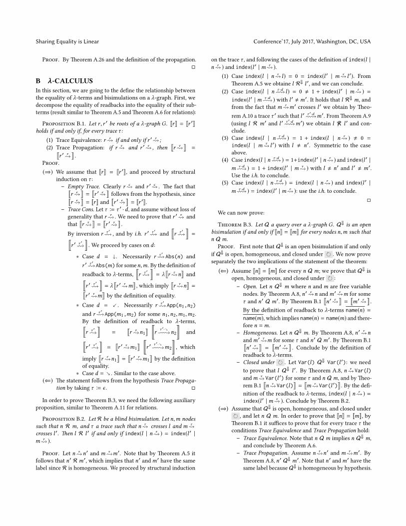
Sharing Equality is Linear Conference’17, July 2017, Washington, DC, USA

Proof. By eorem A.26 and the denition of the propagation.

B λ-CALCULUSIn this section, we are going to the dene the relationship between

the equality of λ-terms and bisimulations on a λ-graph. First, we

decompose the equality of readbacks into the equality of their sub-

terms (result similar to eorem A.5 and eorem A.6 for relations):

Proposition B.1. Let r , r ′ be roots of a λ-graph G. JrK = Jr ′Kholds if and only if, for every trace τ :

(1) Trace Equivalence: r τif and only if r ′ τ

;

(2) Trace Propagation: if r τand r ′ τ

, then

qr τ

y=q

r ′ τy

.

Proof.

(⇒) We assume that JrK = Jr ′K, and proceed by structural

induction on τ :

– Empty Trace. Clearly r ϵand r ′ ϵ

. e fact thatqr ϵ

y=qr ′ ϵ

yfollows from the hypothesis, sinceq

r ϵy= JrK and

qr ′ ϵ

y= Jr ′K.

– Trace Cons. Let τ B τ ′ ·d , and assume without loss of

generality that r τ. We need to prove that r ′ τ

and

that

qr τ

y=qr ′ τ

y.

By inversion r τ ′, and by i.h. r ′ τ ′

and

rr τ ′

z=

rr ′ τ ′

z. We proceed by cases on d :

∗ Case d =

. Necessarily r τ ′ Abs(n) and

r ′ τ ′ Abs(m) for somen,m. By the denition of

readback to λ-terms,

rr τ ′

z= λ

qr τ n

yand

rr ′ τ ′

z= λ

qr ′ τ m

y, which imply

qr τ n

y=

qr ′ τ m

yby the denition of equality.

∗ Case d =. Necessarily r τ ′ App(n1,n2)

and r τ ′ App(m1,m2) for some n1,n2,m1,m2.

By the denition of readback to λ-terms,

rr τ ′

z=

qr τ n1

y sr

τ ′·n2

and

rr ′ τ ′

z=

qr ′ τ m1

y sr ′

τ ′·m2

, which

imply

qr τ n1

y=qr ′ τ m1

yby the denition

of equality.

∗ Case d = . Similar to the case above.

(⇐) e statement follows from the hypothesis Trace Propaga-

tion by taking τ B ϵ .

In order to prove eorem B.3, we need the following auxiliary

proposition, similar to eorem A.11 for relations.

Proposition B.2. Let R be a blind bisimulation. Let n,m nodes

such that n R m, and τ a trace such that n τcrosses l and m τ

crosses l ′. en l R l ′ if and only if index(l | n τ ) = index(l ′ |m τ ).

Proof. Let n τ n′ and m τ m′. Note that by eorem A.5 it

follows that n′ R m′, which implies that n′ andm′ have the same

label since R is homogeneous. We proceed by structural induction

on the trace τ , and following the cases of the denition of index(l |n τ ) and index(l ′ | m τ ).

(1) Case index(l | n τ l) = 0 = index(l ′ | m τ l ′). From

eorem A.5 we obtaine l R⇓ l ′, and we can conclude.

(2) Case index(l | n τ ·d l) = 0 , 1 + index(l ′ | m τ ) =index(l ′ | m τ ·d ) with l ′ ,m′. It holds that l R⇓ m, and

from the fact that m τ m′ crosses l ′ we obtain by eo-

rem A.10 a trace τ ′ such that l ′ τ ′·d m′. From eorem A.9

(using l R m′ and l ′ τ ′·d m′) we obtain l 6R l ′ and con-

clude.

(3) Case index(l | n τ ·d ) = 1 + index(l | n τ ) , 0 =

index(l | m τ l ′) with l , n′. Symmetric to the case

above.

(4) Case index(l | n τ ·d ) = 1+index(l ′ | n τ ) and index(l ′ |m τ ·d ) = 1 + index(l ′ | m τ ) with l , n′ and l ′ , m′.Use the i.h. to conclude.

(5) Case index(l | n τ ·d ) = index(l | n τ ) and index(l ′ |m τ ·d ) = index(l ′ | m τ ): use the i.h. to conclude.

We can now prove:

Theorem B.3. Let Q a query over a λ-graph G. Q⇓ is an open

bisimulation if and only if JnK = JmK for every nodes n,m such that

n Q m.

Proof. First note that Q⇓ is an open bisimulation if and only

if Q⇓ is open, homogeneous, and closed under . We now prove

separately the two implications of the statement of the theorem:

(⇐) Assume JnK = JmK for every n Q m; we prove that Q⇓ is

open, homogeneous, and closed under :

– Open. Let n Q⇓ m where n and m are free variable

nodes. By eorem A.8, n′ τ n andm′ τ m for some

τ and n′ Q m′. By eorem B.1

qn′ τ

y=qm′ τ

y.

By the denition of readback to λ-terms name(n) =name(m), which implies name(n) = name(m) and there-

fore n =m.

– Homogeneous. Let n Q⇓ m. By eorem A.8, n′ τ n

andm′ τ m for some τ and n′ Q m′. By eorem B.1qn′ τ

y=qm′ τ

y. Conclude by the denition of

readback to λ-terms.

– Closed under . Let Var(l) Q⇓ Var(l ′): we need

to prove that l Q⇓ l ′. By eorem A.8, n τ Var(l)andm τ Var(l ′) for some τ and n Q m, and by eo-

rem B.1

qn τ Var(l)

y=qm τ Var(l ′)

y. By the de-

nition of the readback to λ-terms, index(l | n τ ) =index(l ′ | m τ ). Conclude by eorem B.2.

(⇒) Assume that Q⇓ is open, homogeneous, and closed under

, and let n Q m. In order to prove that JnK = JmK, by

eorem B.1 it suces to prove that for every trace τ the

conditions Trace Equivalence and Trace Propagation hold:

– Trace Equivalence. Note that n Q m implies n Q⇓ m,

and conclude by eorem A.6.

– Trace Propagation. Assume n τ n′ and m τ m′. By

eorem A.8, n′ Q⇓ m′. Note that n′ andm′ have the

same label because Q⇓ is homogeneous by hypothesis.

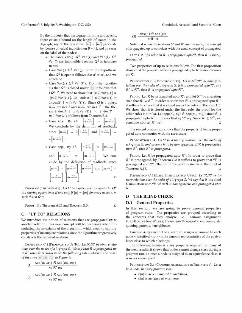
Conference’17, July 2017, Washington, DC, USA Condoluci, Accaoli and Sacerdoti Coen

By the property that the λ-graph is nite and acyclic,

there exists a bound on the length of traces in the

λ-graph, say B. e proof that Jn′K = Jm′K proceeds

by (course of value) induction on B − |τ |, and by cases

on the label of the nodes:

∗ e cases Var() Q⇓ Var(l) and Var(l) Q⇓Var() are impossible because Q⇓ is homoge-

neous.

∗ Case Var() Q⇓ Var(). From the hypothesis

that Q⇓ is open it follows that n′ =m′, and we

conclude.

∗ Case Var(l) Q⇓ Var(l ′). From the hypothe-

sis that Q⇓ is closed under it follows that

l Q⇓ l ′. We need to show that

qn τ Var(l)

y=q

m τ Var(l ′)y

, i.e. index(l | n τ Var(l)) =index(l ′ | m τ Var(l ′)). Since Q is a query,

n τcrosses l and m τ

crosses l ′. e the-

sis index(l | n τ Var(l)) = index(l ′ |m τ Var(l ′)) follows from eorem B.2.

∗ Case Abs. By i.h.

rn

τ ·

z=

rm

τ ·

z.

We conclude by the denition of readback,

since

qn τ

y= λ

rn

τ ·

zand

rm

τ ·

z=

λrm

τ ·

z.

∗ Case App. By i.h.

sn

τ ·

=

sm

τ ·

and

sn

τ ·=

sm

τ ·

. We con-

clude by the denition of readback, since

qn τ

y=

sn

τ · s

nτ ·

and

qm τ

y=

sm

τ · s

mτ ·

.

Proof of (Theorem 4.9). Let Q be a query over a λ-graph G . Q#

is a sharing equivalence if and only if JnK = JmK for every nodes n,msuch that n Q m.

Proof. By eorem A.25 and eorem B.3.

C “UP TO” RELATIONSWe introduce the notion of relations that are propagated up to

another relation. is new concept will be necessary when for-

mulating the invariants of the algorithm, which need to capture

properties of incomplete relations since the algorithm progressively

constructs the required relations.

Definition C.1 (Propagated Up To). Let R,R ′ be binary rela-

tions over the nodes of a λ-graph G. We say that R is propagated up

to R ′ when R is closed under the following rules (which are variants

of the rules

in Figure 3):

(1)

App(n1,n2) R App(m1,m2)

n1 R ′ m1

(2)

App(n1,n2) R App(m1,m2)

n2 R ′ m2

(3)

Abs(n) R Abs(m)

n R ′ mNote that when the relations R and R ′ are the same, the concept

of propagated up to coincides with the usual concept of propagated:

Fact C.2. If a relation R is propagated upto R, then R is simply

propagated.

Two properties of up to relations follow. e rst proposition

shows that the property of being propagated uptoR ′ is monotonous

on R ′.

Proposition C.3 (Monotonicity). Let R,R ′,R ′′ be binary re-

lations over the nodes of a λ-graphG . If R is propagated upto R ′, and

R ′ ⊆ R ′′, then R is propagated upto R ′′.

Proof. Let R be propagated upto R ′, and let R ′′ be a relation

such that R ′ ⊆ R ′′. In order to show that R is propagated upto R ′′,it suces to check that it is closed under the rules of eorem C.1.

We show that it is closed under the rst rule, the proof for the

other rules is similar. Let App(n1,n2) R App(m1,m2); since R is

propagated upto R ′, it follows that n1 R ′ m1. Since R ′ ⊆ R ′′, we

conclude with n1 R ′′ m1.

e second proposition shows that the property of being propa-

gated upto commutes with the rst-closure.

Proposition C.4. Let R be a binary relation over the nodes of

a λ-graph G, and assume R to be homogeneous. If R is propagated

upto R∗, then R∗ is propagated.

Proof. Let R be propagated upto R∗. In order to prove that

R∗ is propagated, by eorem C.2 it suces to prove that R∗ is

propagated upto R∗. e rest of the proof is similar to the proof of

eorem A.16.

Definition C.5 (Blind Bisimulation Upto). Let R,R ′ be bi-

nary relations over the nodes of a λ-graphG . We say that R is a blind

bisimulation upto R ′ when R is homogeneous and propagated upto

R ′.

D THE BLIND CHECKD.1 General PropertiesIn this section, we are going to prove general properties

of program runs. e properties are grouped according to

the concepts that they analyse, i.e. canonic assignment,

BuildEquivalenceClass, EnqueueAndPropagate, enqueuing, de-

queuing, parents, ∼neighbours.

Canonic Assignment. e algorithm assigns a canonic to each

node n: intuitively, c(n) is the canonic representative of the equiva-

lence class to which n belongs.

e following lemma is a key property required by many of

the next results: it shows that nodes cannot change class during a

program run, i.e. once a node is assigned to an equivalence class, it

is never re-assigned.

Proposition D.1 (Canonic Assignment is Definitive). Let nbe a node. In every program run:

• c(n) is never assigned to undened;

• c(n) is assigned at most once.

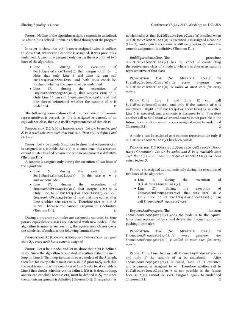
Sharing Equality is Linear Conference’17, July 2017, Washington, DC, USA

Proof. No line of the algorithm assigns a canonic to undened,

i.e. aer c(n) is dened, it remains dened throughout the program

run.

In order to show that c(n) is never assigned twice, it suces

to show that, whenever a canonic is assigned, it was previously

undened. A canonic is assigned only during the execution of two

lines of the algorithm:

• Line 5, during the execution of

BuildEquivalenceClass(c) that assigns c(c) B c .

Note that only Line 3 and Line 12 can call

BuildEquivalenceClass, and both lines check be-

forehand whether the canonic of c is undened.

• Line 27, during the execution of

EnqueueAndPropagate(m, c) that assigns c(m) to c .

Only Line 16 can call EnqueueAndPropagate, and that

line checks beforehand whether the canonic of m is

undened.

e following lemma shows that the mechanism of canonic

representatives is correct, i.e. if c is assigned as canonic of an

equivalence class, then c is itself a representative of that class:

Proposition D.2 (c(·) is Idempotent). Let c,n be nodes, and

S be a reachable state such that c(n) = c . en c(c) is dened and

c(c) = c .

Proof. Let n be a node. It suces to show that whenever c(n)is assigned to c , it holds that c(c) = c; once true, this assertion

cannot be later falsied because the canonic assignment is denitive

(eorem D.1).

A canonic is assigned only during the execution of two lines of

the algorithm:

• Line 5, during the execution of

BuildEquivalenceClass(c). In this case n = cand we conclude.

• Line 27, during the execution of

EnqueueAndPropagate(m,c) that assigns c(m) to c .

Only Line 16 of BuildEquivalenceClass(c) can call

EnqueueAndPropagate(m, c), and that line comes aer

Line 5 which sets c(c) to c . erefore c(c) = c in Sas well, because the canonic assignment is denitive

(eorem D.1).

During a program run nodes are assigned a canonic, i.e. tem-

porary equivalence classes are extended with new nodes. If the

algorithm terminates successfully, the equivalence classes cover

the whole set of nodes, as the following lemma shows:

Proposition D.3 (Canonic Assignment Completed). In a nal

state Sf , every node has a canonic assigned.

Proof. Let n be a node, and let us show that c(n) is dened

in Sf . Since the algorithm terminated, execution exited the main

loop on Line 2. at loop iterates on every node n of the λ-graph,

therefore for every n there must exist a stateS prior toSf such that

the next transition is the execution of Line 3 with local variable n.

Line 3 rst checks whether c(n) is dened. If it is, it does nothing,

and we can conclude because c(n) must be dened in Sf too since

the canonic assignment is denitive (eorem D.1). If instead c(n) is

not dened inS, then BuildEquivalenceClass(n) is called; when

BuildEquivalenceClass(n) is executed, n is assigned a canonic

(Line 5), and again the canonic is still assigned in Sf since the

canonic assignment is denitive (eorem D.1).

BuildEquivalenceClass. e procedure

BuildEquivalenceClass(c) has the eect of constructing

the equivalence class of a node c , where c is chosen as canonic

representative of that class.

Proposition D.4 (No Multiple Calls to

BuildEquivalenceClass(n)). In every program run,

BuildEquivalenceClass(n) is called at most once for every

node n.

Proof. Only Line 3 and Line 12 can call

BuildEquivalenceClass(n), and only if the canonic of n is

undened. Right aer BuildEquivalenceClass(n) is called,

Line 5 is executed, and a canonic is assigned to n. erefore

another call to BuildEquivalenceClass(n) is not possible in the

future, because c(n) cannot be ever assigned again to undened

(eorem D.1).

A node c can be assigned as a canonic representative only if

BuildEquivalenceClass(c) has been called:

Proposition D.5 (Only BuildEquivalenceClass(c) Desig-

nates Canonics). Let c,n be nodes, and S be a reachable state

such that c(n) = c . en BuildEquivalenceClass(c) has been

called before S.

Proof. c is assigned as a canonic only during the execution of

two lines of the algorithm:

• Line 5, during the execution of

BuildEquivalenceClass(c).

• Line 27, during the execution of

EnqueueAndPropagate(m,c) that sets c(m) to c .

Only Line 16 of BuildEquivalenceClass(c) can

call EnqueueAndPropagate(m,c).

EnqueueAndPropagate. e function

EnqueueAndPropagate(m,c) adds the node m to the equiva-

lence class represented by c , and delays the processing of m by

pushing it into q(c).

Proposition D.6 (No Multiple Calls to

EnqueueAndPropagate(n,–)). In every program run,

EnqueueAndPropagate(n,–) is called at most once for every

node n.

Proof. Only Line 16 can call EnqueueAndPropagate(m, c),and only if the canonic of m is undened. Aer

EnqueueAndPropagate(m,c) is called, Line 27 is executed,

and a canonic is assigned to m. erefore another call to

BuildEquivalenceClass(m,–) is not possible in the future,

because c(m) cannot be ever assigned again to undened

(eorem D.1).

Conference’17, July 2017, Washington, DC, USA Condoluci, Accaoli and Sacerdoti Coen

Enqueuing. Two lines of the algorithm push a node to a queue:

Line 7, when q(c) is created and c pushed to it; Line 28, whenm is

pushed to q(c). Intuitively, pushing a node to q(c) results in delaying

its processing by the algorithm; the node will be fully processed

only later, aer being popped from the queue (Lines 9–17).

Proposition D.7 (Enqeue Once). In a program run, every node

n is enqueued at most once.

Proof. e algorithm enqueues a node only shortly aer seing

its canonic:

• on Line 7, aer assigning a canonic on Line 5;

• on Line 28, right aer assigning a canonic on Line 27.

Since the canonic of a node can be assigned at most once (eo-

rem D.1), it follows that a node can be enqueued at most once.

e following lemma shows that q(c) is a subset of the equiva-

lence class with canonic representative c:

Proposition D.8 (eue ⊆ Eqivalence Class). Let S be a

reachable state, and n a node. If n ∈ q(c), then c(n) is dened and

c(n) = c .

Proof. Let n be a node. Since the canonic assignment is deni-

tive (eorem D.1), it suces to check that c(n) = c whenever n is

enqueued to q(c). A node is enqueued only during the execution of

two lines of the algorithm:

• Line 7 during the execution of

BuildEquivalenceClass(c). In this case n = c ,

and the canonic of c was just assigned to c itself on Line 5.

• Line 28 during the execution of

EnqueueAndPropagate(m, c). Line 28 is executed

right aer Line 27, which sets c(m) B c .

Dequeuing. Nodes are popped from a queue only on Line 9. Once

a node is dequeued, the algorithm proceeds by rst visiting its

parents (Line 10) and then its ∼neighbours (Line 14).

Proposition D.9 (Deqeued Nodes Have Correct Canonic).

Let S be a state reached aer the execution of Line 9 with locals c,n.

en c(n) is dened and c(n) = c .

Proof. Let n be a node. n ∈ q(c) in the state S′ right before the

execution of Line 9 with locals c,n. erefore c(n) = c in S′ by

eorem D.8. Conclude with c(n) = c in S because the canonic

assignment is denitive (eorem D.1).

Definition D.10 (Processed Node). In a reachable state S, we

say that a node n has already been processed if Lines 9–17 with locals

c,n have already been executed (for some c).

In other words, a node n is processed aer it is dequeued and its

parents and ∼neighbours visited.

Aer BuildEquivalenceClass(c) returns, all the nodes in the

equivalence class of c are processed:

Proposition D.11 (Eqivalence Class Processed).

Let c,n be nodes, and S a reachable state such that

BuildEquivalenceClass(c) has already returned. If c(n) = c ,

then n is processed.

Proof. c(n) is assigned to c only during the execution of

BuildEquivalenceClass(c) (eorem D.5). First, note that

shortly aer c(n) is assigned to c (Line 5 or Line 27), n is enqueued

to q(c) (resp. Line 7 and Line 28).

In both cases, n is enqueued to q(c) when the execution of the

while loop on Line 8 has not terminated yet: on Line 7 before the

beginning of the loop, on Line 28 during the execution of the loop,

since EnqueueAndPropagate is called from Line 16 which is inside

the while loop.

Note also that a node n is dequeued from q(c) only on Line 9

during the execution of BuildEquivalenceClass(c), and that

BuildEquivalenceClass(c) can be called at most once (eo-

rem D.4).

In conclusion, n was enqueued to q(c) before the com-

pletion of the while loop on q(c) on Line 8, and since

BuildEquivalenceClass(c) has already returned and the while

loop terminated, at some point n was dequeued from q(c) on Line 9,

and the body of the loop executed with locals c,n.

Proposition D.12 (Deqeue Once). In each program run, Line 9

is executed with local n at most once for every node n.

Proof. Executing Line 9 with local n dequeues n, which cannot

be enqueued twice by eorem D.7.

Parents. e loop on Line 10 iterates on all the parents of a node,

building their equivalence classes:

Proposition D.13 (Parent Classes Built). Let c,n be nodes,

and letS be a state reachable aer the execution of the loop on Line 10

of BuildEquivalenceClass(c) with local variables c,n. en for

every parentm of n:

• c(m) is dened, say c(m) = c ′;• BuildEquivalenceClass(c ′) has been called and has al-

ready returned.

Proof. e loop on Line 10 iterates on all parents of n. For

every parentm:

• If m has no canonic assigned,

BuildEquivalenceClass(m) is called (Line 12). Since

S is reached aer the execution of the loop, the call

to BuildEquivalenceClass(m) has already returned.

Note that m was assigned itself as a canonic on Line 5

of BuildEquivalenceClass(m), and c(m) =m still in S(eorem D.1).

• Ifm has some c ′ assigned as a canonic node, then Line 13

enforces that building(c ′) = false. is means that

Line 18 of BuildEquivalenceClass(c ′) has already been

executed, and therefore BuildEquivalenceClass(c ′) has

already returned.

∼neighbours. e loop on Line 14 iterates on all the ∼neighbours

of a node. Note that the loop does not remove ∼edges aer iterating

on them: in fact, the algorithm simply ignores ∼edges that have

already been encountered, as it calls EnqueueAndPropagate only

on ∼neighbours that have not been enqueued yet (Line 16).

Proposition D.14 (∼ Grows). During a program run, ∼ mono-

tonically grows.

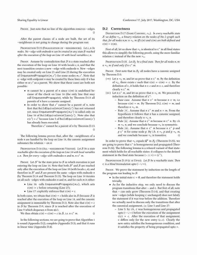
Sharing Equality is Linear Conference’17, July 2017, Washington, DC, USA

Proof. Just note that no line of the algorithm removes ∼edges.

Aer the parent classes of a node are built, the set of its

∼neighbours is not going to change during the program run:

Proposition D.15 (Finalization of ∼neighbours). Let c,n be

nodes. No ∼edge with endnode n can be created in any stateS reached

aer the execution of the loop on Line 10 with local variables c,n.

Proof. Assume by contradiction that S is a state reached aer

the execution of the loop on Line 10 with locals c,n, and that the

next transition creates a new ∼edge with endnode n. New ∼edges

may be created only on Line 21 and Line 23 during the execution

of EnqueueAndPropagate(m, c ′) for some nodes m, c ′. Note that

a ∼edge with endpoint n may be created by these lines only if n has

eitherm or c ′ as a parent. We show that these cases are both not

possible:

• m cannot be a parent of n since c(m) is undened be-

cause of the check on Line 16 (the only line that may

call EnqueueAndPropagate), while by eorem D.13 all

parents of n have a canonic assigned.

• In order to show that c ′ cannot be a parent of n, note

rst that BuildEquivalenceClass(c’) has not returned

yet, since EnqueueAndPropagate(m,c’) is called only on

Line 16 of BuildEquivalenceClass(c’). Note also that

c(c ′) = c ′ because Line 5 of BuildEquivalenceClass(c’)has already been executed.

erefore c ′ cannot be a parent of n by eorem D.13.

e following lemma proves that, aer the ∼neighbours of a

node n are handled by the loop on Line 14, the canonic assignment

subsumes the relation ∼ on n:

Proposition D.16 (All ∼neighbours Visited). Let S be a state

reachable aer the execution of the loop on Line 14 with local variables

c,n. en for every ∼edge with endnodes n andm, n c∗ m.

Proof. Let S′ be the state prior to S in which execution is just

entering the loop on Line 14. Note that both S′ and S are reached

only aer the execution of the loop on Line 10 (with locals c,n), and

therefore in S′ and S are present the same ∼edges with endnode n(by eorem D.14 and eorem D.15). e loop on Line 14 iterates

on all such ∼edges with endnodes n andm, and for eachm it either:

• Line 16: calls EnqueueAndPropagate(m,c), which sets

c(m) B c before returning (Line 27);

• Line 17: explicitly enforces that c(m) = c .

In both cases, we obtain that c(m) = c holds also in S (because S is

reached aer the execution of the loop on Line 14, and the canonic

assignment is immutable by eorem D.1). Note also that c(n) = cin S by eorem D.9, since S is reached aer the execution of

Line 9 which dequeues n from q(c).We thus obtain c(n) = c(m) = c in S, i.e. n c∗ m.

In the following sections, we are going to prove that Algorithm 1

is sound (Appendix D.2), complete (Appendix D.3), and that it runs

in linear time (Appendix D.4).

D.2 CorrectnessDefinition D.17 (Same Canonic, =c). In every reachable state

S we dene =c, a binary relation on the nodes of the λ-graph such

that, for all nodes n,m: n =c m i c(n) and c(m) are both dened and

c(n) = c(m).

First of all, let us show that =c is identical to c∗ in all nal states:

this allows to simplify the following proofs, using the more familiar

relation c instead of the the new =c.

Proposition D.18. Let Sf be a nal state. en for all nodes n,m:

n =c m if and only if n c∗ m.

Proof. First note that in Sf all nodes have a canonic assigned

by eorem D.3.

(⇒) Let n =c m, and let us prove that n c∗ m. By the denition

of =c, there exists c such that c(n) = c(m) = c . By the

denition of c, it holds that n c c andm c c , and therefore

clearly n c∗ m.

(⇐) Let n c∗ m, and let us prove that n =c m. We proceed by

induction on the denition of c∗:– Base case. Assume that n c∗ m because n c m, i.e.

because c(n) = m. By eorem D.2, c(m) = m, and

therefore n =c m.

– Rule • . Assume that n c∗ m and n = m. From the

hypothesis it follows that n has a canonic assigned,

and therefore clearly n =c n.

– Rule . Assume that n c∗ m because m c∗ n. By i.h.

m =c n, and we conclude because =c is symmetric.

– Rule . Assume that n c∗ m because n c∗ p and

p c∗ m for some node p. By i.h. n =c p and p =c m,

and we conclude because =c is transitive.

In order to prove that =c equals Q#in Sf (eorem D.25), we

are going to prove that c∗ is homogeneous and propagated (eo-

rem D.24). e following lemma is a relaxed variant of that state-

ment which holds for all reachable states: it collapses to the desired

statement in the nal state because (∼ ∪ =) = (c∗).

Proposition D.19 (c is Upto). Let S be a reachable state. en

c is a blind bisimulation upto (∼ ∪ =).

Proof. We prove the statement by induction on the length of

the program run leading to S:

• In the initial state c = ∅, and therefore the statement holds

trivially.

• As for the inductive step, we only need to discuss the

program transitions that alter ∼ and c. But rst of all, note

that ∼ can only grow (eorem D.14), and that creating

new ∼edges (while keeping c unchanged) does not falsify

the statement if it was true before the addition. erefore

we actually need to discuss only the transitions that alter

the canonical assignment, i.e. Line 5 and Line 27:

– Line 5: by i.h., c was homogeneous and propagated

upto (∼ ∪ =) before the execution of the assignment

c(c) = c . Aer the execution of that assignment,

c diers only for the new entry (c, c). Clearly the

new entry satises the homogeneous condition, and

it satises the property of being propagated upto =.

Conference’17, July 2017, Washington, DC, USA Condoluci, Accaoli and Sacerdoti Coen

– Line 27, during the execution of

EnqueueAndPropagate(m, c): by i.h., c was

homogeneous and propagated upto (∼ ∪ =) before

the execution of the assignment c(m) B c . Aer

the execution of that assignment, c diers only for

the new entry (m, c). e new entry satises the

homogeneous condition and the property of being

propagated upto ∼ because of the code executed in

Lines 20–26, which checked the labels of the nodes

and created ∼edges on the corresponding children of

m, c if any.

e following eorem D.20 and eorem D.21 state properties

that connect the relations c, Q, and ∼. In a nal state c∗ is exactly

∼∗, but in intermediate states the following weaker property holds:

Proposition D.20. In every reachable state S: c ⊆ ∼∗.

Proof. We prove the statement by induction on the length of

the program run leading to S:

• In the initial state, c = ∅ and therefore the statement holds

trivially.

• As for the inductive step, we only need to discuss the

program transitions that alter ∼ and c. But rst of all,

note that during the execution of the algorithm ∼ can

only grow (eorem D.14), and that creating new ∼edges

(while keeping c unchanged) does not falsify the statement

if it was true before the addition. erefore we actually

need to discuss only the transitions that alter the canonical

assignment, i.e. Line 5 and Line 27:

– Line 5: by i.h., c ⊆ ∼∗ before the execution of the as-

signment c(c) = c . Aer the execution of that assign-

ment, c diers only for the new entry (c, c). Clearly

c ∼∗ c because ∼∗ is reexive by denition.

– Line 27, during the execution of

EnqueueAndPropagate(m, c): by i.h., c ⊆ ∼∗before the execution of the assignment c(m) B c .

Aer the execution of that assignment, c dif-

fers only for the new entry (m, c). Note that

EnqueueAndPropagate(m, c) is called from Line 16

during the execution of BuildEquivalenceClass(c).

Because of the loop on Line 14,m was a ∼neighbour

of n for some node n, and it still is because ∼ can only

grow (eorem D.14). We are now going to prove

that n ∼∗ c , which together with the fact that m is

a ∼neighbour of n, will allow us to conclude with

m ∼∗ c .

Line 16 is executed aer Line 9, therefore c(n) = c (i.e.

n c c) by eorem D.9. By i.h. n c c implies n ∼∗ c ,

and we are done.

During a program run, the relation∼ progressively approximates

the relation Q#:

Proposition D.21 (∼ Approximates Q#). In every reachable

state S: Q ⊆ ∼ ⊆ Q#.

Proof. We prove the statement by induction on the length of

the execution trace leading to S:

• Base case. In the initial state (∼) = Q and the statement

clearly holds.

• Inductive step. First note that during the execution of

the algorithm ∼ can only grow (eorem D.14), therefore

the requirement Q ⊆ ∼ follows from the i.h. In order to

prove that ∼ ⊆ Q#, we only need to discuss the program

transitions that alter ∼, i.e. those occurring on Line 21 and

Line 23:

– Line 21 during the execution of

EnqueueAndPropagate(m,c). Because of the check

on the same line, m = Abs(m′) and c = Abs(c ′) for

somem′, c ′. Executing Line 21 creates the new edge

m′ ∼ c ′. Since Q#is propagated, in order to show

the new requirement m′ Q# c ′ it suces to show

that m Q# c . We are going to show that m ∼∗ c in

the state prior to S: then by using the i.h. we obtain

m Q# c , and we can conclude.

Note that EnqueueAndPropagate(m, c) is

called from Line 16 during the execution of

BuildEquivalenceClass(c). Because of the loop on

Line 14, m was a ∼neighbour of n for some node n,

and it still is because ∼ can only grow (eorem D.14).

In order to prove m ∼∗ c , it thus suces to prove

n ∼∗ c . e laer follows from eorem D.20, by

using the fact that Line 16 is executed aer Line 9,

therefore c(n) = c– Line 23 is similar to the previous case.

Corollary D.22. In every reachable state, c∗ ⊆ Q#.

Proposition D.23 (All ∼edges Visited). In every nal state,

(∼) ⊆ (c∗).

Proof. Let Sf be a nal state. By eorem D.3, in Sf every

node has a canonic assigned. Let n be a node, and c B c(n); we are

going to prove that n c∗ m for every ∼neighbourm of n.

By eorem D.5, BuildEquivalenceClass(c) was called before

Sf . Since Sf is nal, BuildEquivalenceClass(c) must have re-

turned, and therefore n has already been processed (eorem D.11).

Aer the loop on Line 10, the ∼neighbours of n are nalized (eo-

rem D.15), and aer the loop on Line 14, the ∼neighbours of n are

all visited (eorem D.16).

Proposition D.24. Let Sf a nal state. en c∗ is a blind bisim-

ulation.

Proof. By eorem D.19, c is homogeneous and propagated up

to (∼∪=). We need to show that c∗ is homogeneous and propagated.

• Homogeneous. It follows from eorem A.15.

• Propagated. By eorem D.23 and eorem D.18, (∼) ⊆(c∗), which implies that (∼ ∪ =) ⊆ (c∗) because c∗ is re-

exive. erefore c is propagated up to c∗ by eorem C.3,

and c∗ is propagated by eorem C.4.

Proposition D.25. Let Sf a nal state. en (c∗) = (Q#).

Proof. By eorem D.22, (c∗) ⊆ (Q#). In order to prove (Q#

) ⊆ (c∗), it suces to note that Q ⊆ (c∗) (because Q ⊆ (∼)by eorem D.21, and (∼) ⊆ (c∗) by eorem D.23), that c∗ is

Sharing Equality is Linear Conference’17, July 2017, Washington, DC, USA

an equivalence relation (by denition), and that c∗ is propagated

(eorem D.24).

Proof of (Theorem 6.1). In every nal state Sf :

• Succint representation: (=c) = (Q#),• Blind check: Q#

is homogeneous, and therefore a blind shar-

ing equivalence.

Proof. By eorem D.24 and eorem D.25.

D.3 CompletenessDefinition D.26 (Staircase Order ≺). Let S be a reachable

state, and n,m be nodes of the λ-graphG . We say that n ≺m i there

exist a direction d and a node p such that m d p (riser) and p c n(tread).

Proposition D.27 (Order of Active Classes). LetS be a reach-

able state such that active = [c1, . . . , cK ]. en ci ≺ ci+1 for every

0 < i < K .

Proof. We proceed by induction on the length of the program

run. In the base case, i.e. in the initial state, the callstack is empty

and therefore the property holds trivially.

As for the inductive step, we only need to discuss the pro-

gram transitions that actually alter the callstack, i.e. when

BuildEquivalenceClass is called or when it returns:

• BuildEquivalenceClass returns. In this case, the last

entry of the callstack is removed, and the statement follows

from the i.h.

• BuildEquivalenceClass(n) is called (Line 3). Right be-

fore the call to BuildEquivalenceClass(n) the callstack

is empty, and right aer the call active = [n], i.e. there is

nothing to prove.

• BuildEquivalenceClass(m) is called (Line 12). In this

case m is a parent of n (i.e. there exists a direction

d such that m d n), and c = cK before the call to

BuildEquivalenceClass(m). Note that Line 12 is exe-

cuted aer Line 9 with locals c,n, and therefore c(n) = c(eorem D.9).

Aer the call to BuildEquivalenceClass(m),

active = [c1, . . . , cK ,m]. e statement for i < K follows

from the i.h., and for the case i = K we just proved that

m d n and n c cK .

e intuition is that recursive calls to BuildEquivalenceClassclimb a stair of nodes in the λ-graph. e algorithm fails when

it encounters a step that was already climbed: this is because the

staircase order is strict when Q#is homogeneous and propagated.

Proposition D.28 (Q#Respects Staircase Order). Let S be a

reachable state, and let c1, . . . , cK be nodes such that c1 ≺ . . . ≺ cK .

If Q#is homogeneous, then ci Q# c j if and only if i = j.

Proof. If i = j, then clearly ci Q# c j because Q#is reexive.

For the other direction, assume by contradiction and without

loss of generality that i < j (since Q#is symmetric). We are going

to prove that there exist a non-empty trace τ and a node m such

that c jτ m and ci Q# m: this, together with ci Q# c j , will yield a

contradiction by eorem A.9.

We proceed by induction on j − i − 1:

• Case i + 1 = j. Obtain from eorem D.27 a node n and

a direction d such that ci+1 = c jd n and n c ci , and

conclude because ci Q# m by eorem D.22.

• Case i + 1 < j. By i.h. there exist a non-empty trace τ and

a node n such that c jτ n and ci+1 Q# n. By eorem D.27,

there exist a direction d and a nodem such that ci+1

d mand m c ci (and therefore ci Q# m by eorem D.22).

From ci+1 Q# n and ci+1

d m, by eorem A.6 there exists

a nodem′ such thatn d m′ andm Q# m′. We can conclude,

since c jτ ·d m′ and ci Q# m′.

We are now ready to prove that the algorithm is complete:

Theorem D.29 (Completeness). If the algorithm fails, then Q#

is not homogeneous.

Proof. Let S be a failing state, i.e. a reachable state that tran-

sitions to Fail. Let active = [c1, . . . , cK ] in S. ere are three

lines of the algorithm in which failure may occur: Line 13, Line 17,

and Line 26. We discuss these cases separately; in all cases, in

order to prove that Q#is not homogeneous, we assume Q#

to be

homogeneous, and derive a contradiction.

• Line 13. Let m be a parent of n such that c(m) = c ′ and

building(c ′) = true. Since building(c ′) = true, the

call to BuildEquivalenceClass(c’) has not returned be-

fore S, and therefore c ′ = ci for some 0 < i ≤ K . By

eorem D.27 c1 ≺ . . . ≺ cK , and therefore c ′ was al-

ready encountered in the stair of active classes. Note that

c(n) = cK = c (eorem D.9), and therefore cK ≺ m. Also,

from c(m) = ci it follows thatm Q# ci (eorem D.22). e

contradiction is obtained by noting that by eorem D.28 it

cannot be the case thatm Q# ci , since c1 ≺ . . . ≺ cK ≺m.

• Line 17. Let m be a ∼neighbour of n such that c(m) =c ′ , c . By eorem D.9, c(n) = c . Since c(m) = c ′,BuildEquivalenceClass(c’) must have been called (e-

orem D.5), and there are two options:

– BuildEquivalenceClass(c’) has already returned.

We show that this is not possible. In fact, if

BuildEquivalenceClass(c’) has returned before

S, then m has already been processed before S(eorem D.11). erefore n =c m (eorem D.16),

contradicting the hypothesis that c , c ′.– BuildEquivalenceClass(c’) has not yet returned.

erefore c ′ = ci for some 0 < i < K . From

c(n) = c = cK and c(m) = ci obtain n ∼∗ cK and

m ∼∗ ci (eorem D.20). Since m is a ∼neighbour of

n, ci ∼∗ cK , and therefore ci Q# cK by eorem D.21.

is yields a contradiction by eorem D.27 and

eorem D.28.

• Line 26. Assume that c and m do not respect the ho-

mogenity condition. We are going to prove that c Q# m,

which contradicts the hypothesis that Q#is homogeneous.

EnqueueAndPropagate(m,c) is called from Line 16, and

thereforem is a ∼neighbour of n. Line 16 is executed aer

Conference’17, July 2017, Washington, DC, USA Condoluci, Accaoli and Sacerdoti Coen

Line 9 with locals c,n, and therefore c(n) = c by eo-

rem D.9. By eorem D.20, c ∼∗ n, and therefore c ∼∗ m.

By eorem D.21, we conclude with c Q# m.

Proof of (Theorem 6.2). If Algorithm 1 fails, then Q#is not a

blind sharing equivalence, and therefore by the blind universality of

Q#(eorem 4.7), there does not exist any blind sharing equivalence

containing the initial query Q.

Proof. By eorem D.29 and eorem 4.7.

D.4 Termination & LinearityIn this section, we are going to show that Algorithm 1 always

terminates within a number of transitions that is linear on the size

of the λ-graph and the initial query Q.

First some notations:

Definition D.30.

• N B nodes(G) is the set of nodes in the λ-graph G• E is the set of directed (

,

, ) edges in the λ-graph

• | · | is the size of a (multi)set.

• #edдes(∼,n) is the number of ∼edges with endnode n. (Recall

that ∼ is a multirelation)

• #parents(n) is the number of directed edges in E with target

n.

e following lemma proves that in every reachable state the

number of query edges is linear in the size of Q and c. e state-

ment of the lemma is actually more complicated, because the proof

requires a more precise bound on |undir|. In particular, the bound

|undir| ≤ 2 × |Q| + 4 × |c | holds in almost every state, but breaks

temporarily during the execution of EnqueueAndPropagate, just

before the execution of Line 27. e problem is that Lines 20–26

may add new ∼edges, while the new canonic that restores the

disequality is only assigned slightly later, on Line 27.

Proposition D.31 (Bound on undir). In every reachable state

S, |undir| ≤ 2 × |Q| + 4 × |N |.

Proof. Proved by induction on the length of the program run

leading to S. In the initial state S0, |undir| = 2 × |Q| because

undir contains the same edges as Q (but undir is also symmetric

and a multirelation, hence each ∼edge counts twice).

During the program run, new ∼edges are created only by the

EnqueueAndPropagate procedure, which may create at most two

new∼edges per call (that count as four new entries of the symmetric

multirelation undir). By eorem D.6, EnqueueAndPropagate is

called at most |N | times in each program run, hence we conclude

with the bound |undir| ≤ 2 × |Q| + 4 × |N |.

Theorem D.32 (Termination & Linearity). In every program

run, the number of transitions is O(|N | + |E | + |Q|).

Proof. Let us assume a program run with end state S (not

necessarily a nal state). We are going to discuss the number of

transitions in the program run in a global way. We group the

transitions in the program run according to which procedure they

are executing a line of, and we discuss the procedures BlindCheck,

BuildEquivalenceClass, and EnqueueAndPropagate separately.

(1) Transitions executing lines of BlindCheck. e proce-

dure BlindCheck() is called exactly once, in the initial

state. e loop on Line 2 simply iterates on all the nodes of

the λ-graph: hence the loop bound is just |N |. Line 3 may

call the procedure BuildEquivalenceClass, but here we

do not consider the transitions caused by that function,

that will be discussed separately below. erefore, the total

number of transitions that execute lines of BlindCheck is

simply O(|N |).(2) Transitions executing lines of EnqueueAndPropagate.

e procedure EnqueueAndPropagate(n,–) is called

at most once for every node n (eorem D.6). Since

EnqueueAndPropagate contains no loops and no function

calls, there is a constant bound on the number of transi-

tions that are executed by EnqueueAndPropagate each

time it is called. erefore, the total number of transitions

that execute lines of EnqueueAndPropagate is O(|N |).(3) Transitions executing lines of BuildEquivalenceClass.

e discussion of the complexity of

BuildEquivalenceClass is more involved, because

it contains multiple nested loops.

As a rst approximation, the total number of transi-

tions executing lines of BuildEquivalenceClass is big-

O of the number of calls to BuildEquivalenceClassplus the numer of transitions executing lines of the loop

on Line 8 (i.e. Lines 8–17). e number of calls to

BuildEquivalenceClass is ≤ |N | (eorem D.4). As for

the loop on Line 8, in every program run the body of the

loop is executed at most once for every node n (eo-

rem D.12).

e body of the while loop contains two additional

loops: one on Line 10, and the other on Line 14:

• e loop on Line 10 (with locals c,n) simply iterates

on all the parents of a node, which is a xed number:

therefore each time it is executed with local variable

n, it is responsible for O(#parents(n)) transitions.

• e discussion about the loop on Line 14 (with locals

c,n) is more involved: it iterates on all ∼neighbours

of a node n, but ∼ changes during the execution

of the loop. In fact, the body of the loop may

call EnqueueAndPropagate(m,c) on Line 16, which

may create new ∼edges. However, note that the

loop on Line 14 is executed only aer the loop on

Line 10, which nalizes the ∼neighbours of n (e-

orem D.15). erefore the loop on Line 14 iterates

on a set of ∼edges that does not change aerwards

during the program run, and is therefore responsible

for O(#edдes(∼,n)) transitions (where the relation ∼is the one in S).

Sharing Equality is Linear Conference’17, July 2017, Washington, DC, USA

erefore the total number of transitions executing

Lines 8–17 is big-O of:∑#parents(n) + #edдes(∼,n) + 1 | Line 9 is executed with local n

≤∑n∈N(#parents(n) + #edдes(∼,n) + 1)

=∑n∈N

#parents(n) +∑n∈N

#edдes(∼,n) +∑n∈N

1

= |E | + |undir| + |N |.Note that by eorem D.31, |undir| ∈ O(|Q| + | |N | |).

erefore the total number of transitions executing lines

of BuildEquivalenceClass in a program run is O(|N | +|E | + |Q|).

In conclusion, we obtain the following asymptotic bound on the

number of transitions in a program run:

O(|N |) +O(|N |) +O(|N | + |E | + |Q|) = O(|N | + |E | + |Q|).

Proof of (Theorem 6.4). Let S0 be an initial state of the al-

gorithm, with a query Q over a λ-graph G. en the Blind check

terminates in a number of transitions linear in |G | and |Q|.

Proof. By eorem D.32.

E THE VARIABLES CHECKProof of. eorem 7.1 Let Q be a query over a λ-graphG passing

the Blind check, and let c be the canonic assignment produced by that

check.

• (Completeness) If the Variables check fails then there are no

sharing equivalences containing Q,

• (Correctness) otherwise =c is the smallest sharing equiva-

lence containing Q.

Moreover, the Variables check clearly terminates in time linear in the

size of G.

Proof. First note that since the Blind Check succeeded, both

c and =c are homogeneous relations. We also use the fact that

(=c) = (c∗) (eorem D.18).

• Completeness: If the Variables Check fails on line 8, then cis not an open relation, and therefore also =c is not open by

eorem A.23. If the Variables Check fails on line 9, then

c is not a bisimulation upto =c, and therefore =c is not a

bisimulation, and therefore it is not a sharing equivalence.

• Correctness: Since also the Variables Check succeeded, c is

an open relation, and closed under upto =c. In order to

show that =c is a sharing equivalence, it suces to show

that it is open, and closed under . =c is closed under

by eorem A.16. =c is open by eorem A.23.

• Termination in linear time: obvious, since the algorithm

simply iterates on all variable nodes of the λ-graph.