Session 5 Handling Data Dec17 · PDF file · 2017-12-19standard deviation (σ)...
61
Level 3 Award in Mathematics for numeracy Teaching: Session 5: Handling data Gail Lydon & Jo Byrne
Transcript of Session 5 Handling Data Dec17 · PDF file · 2017-12-19standard deviation (σ)...
Level 3 Award in Mathematics for numeracy
Teaching:
Session 5: Handling data
Gail Lydon & Jo Byrne
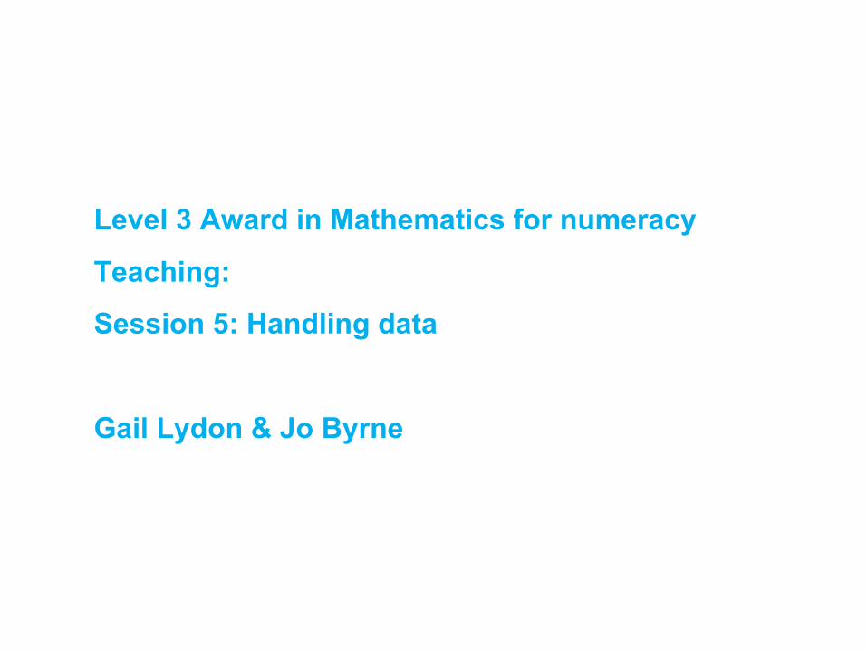
Log into the online page for data handling• Log into the google doc with the answers you have sent
to Jo. We will use that in a little while. https://drive.google.com/drive/folders/12QHkA0-FleJzkF_Zx70LPy_-0Js_O6gV?ths=true
Now:• https://ccpathways.co.uk/level-3-maths-online/• You'll need the password L3Maths16• on the Data Handling button• Read HO1 Data Handling and note on your ILP anything
you need to focus on.
©greatlearning,2017
Session aim
• To review & extend participants’ personal mathematics relating to statistics and probability
• To apply concepts of statistics and probability to solve problems
©greatlearning,2017
What do you need to know about statistics?
©greatlearning,2017
What do you need to know about statistics?
• Mean, median and mode• Sampling techniques• Data transformation (measures of
dispersion, curve fitting, spread, upper and lower quartiles, interquartile range, standard deviation)
• Statistical diagrams• Regression• Correlations• Probability
©greatlearning,2017

Review
• HO1
©greatlearning,2017
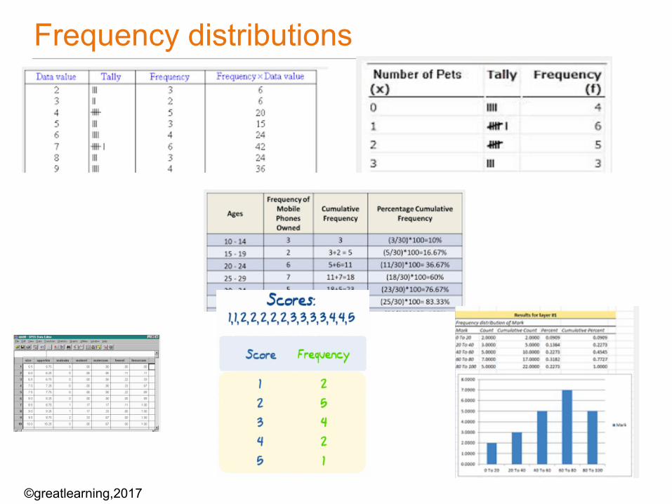
Frequency distributions
©greatlearning,2017
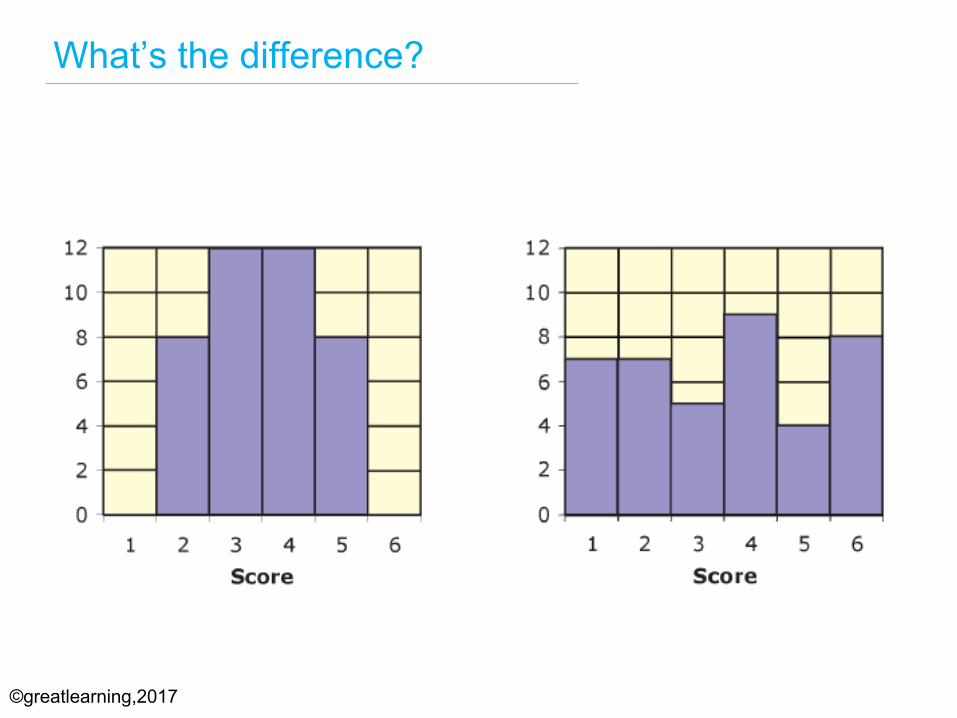
What’s the difference?
©greatlearning,2017
Measures of dispersion
• Range• Interquartile range• Variance• Standard deviation
©greatlearning,2017
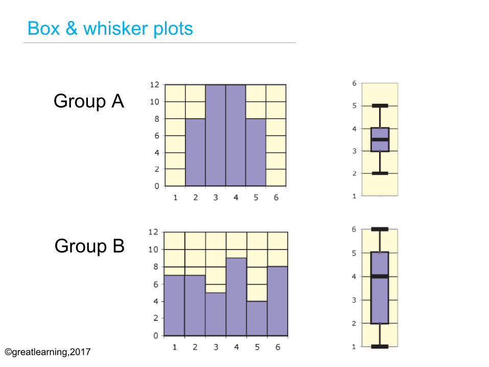
Box & whisker plots
Group A
Group B
©greatlearning,2017
Variance and standard deviation
©greatlearning,2017
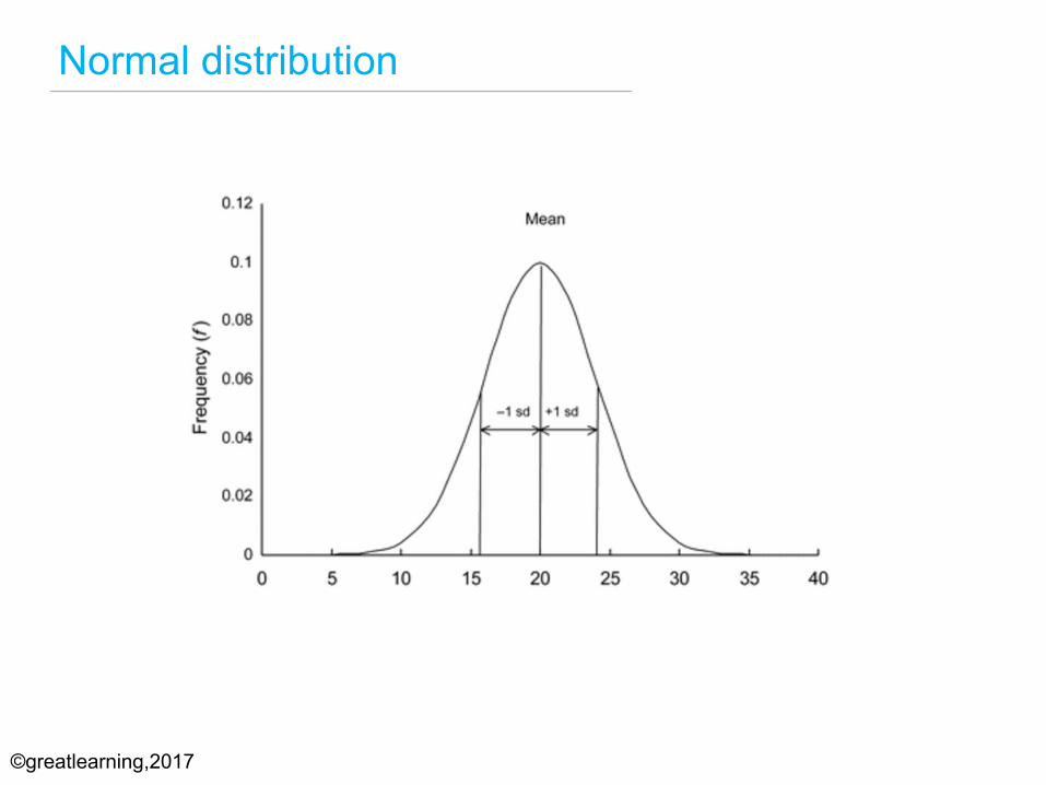
Normal distribution
©greatlearning,2017
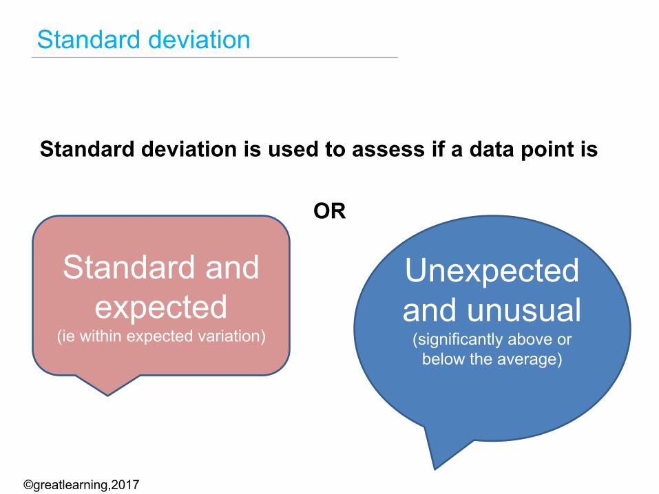
Standard deviation
Standard deviation is used to assess if a data point is
OR
Standard and expected
(ie within expected variation)
Unexpected and unusual
(significantly above or below the average)
©greatlearning,2017
Standard deviation is represented by lower case sigma
𝝈©greatlearning,2017
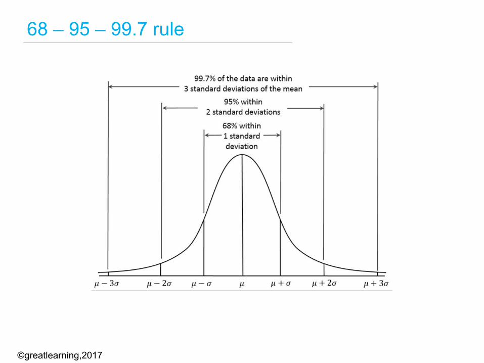
68 – 95 – 99.7 rule
©greatlearning,2017
ΣUpper case sigma
©greatlearning,2017
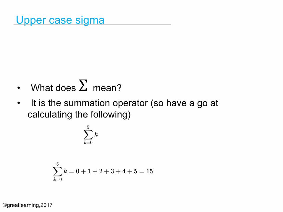
• What does Σ mean?• It is the summation operator (so have a go at
calculating the following)
Upper case sigma
©greatlearning,2017
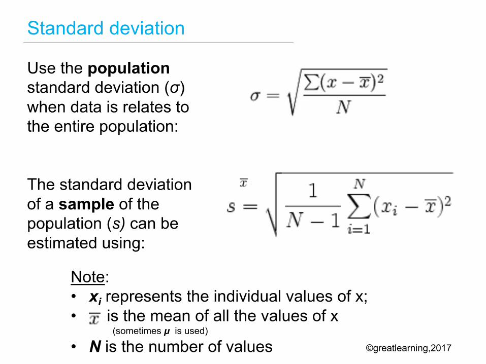
Standard deviation
Use the populationstandard deviation (σ) when data is relates to the entire population:
The standard deviation of a sample of the population (s) can be estimated using:
Note: • xi represents the individual values of x; • is the mean of all the values of x
(sometimes μ is used)
• N is the number of values ©greatlearning,2017
Let’s have a go at a standard deviation problem
• Have a look at HO2 (under R5)
©greatlearning,2017
Grouped and cumulative frequency distributions
©greatlearning,2017
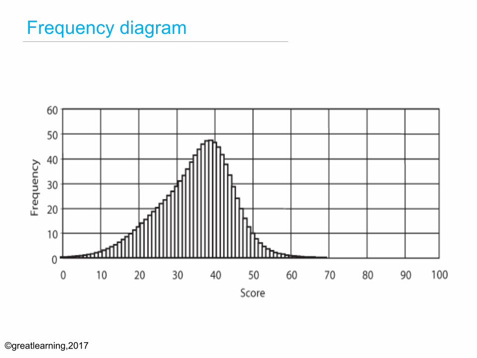
Frequency diagram
©greatlearning,2017
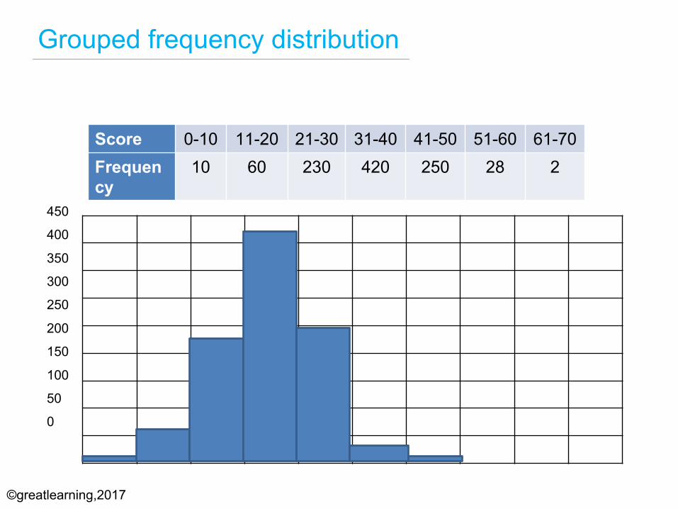
Grouped frequency distribution
450
400
350
300
250
200
150
100
50
0
Score 0-10 11-20 21-30 31-40 41-50 51-60 61-70Frequency
10 60 230 420 250 28 2
©greatlearning,2017
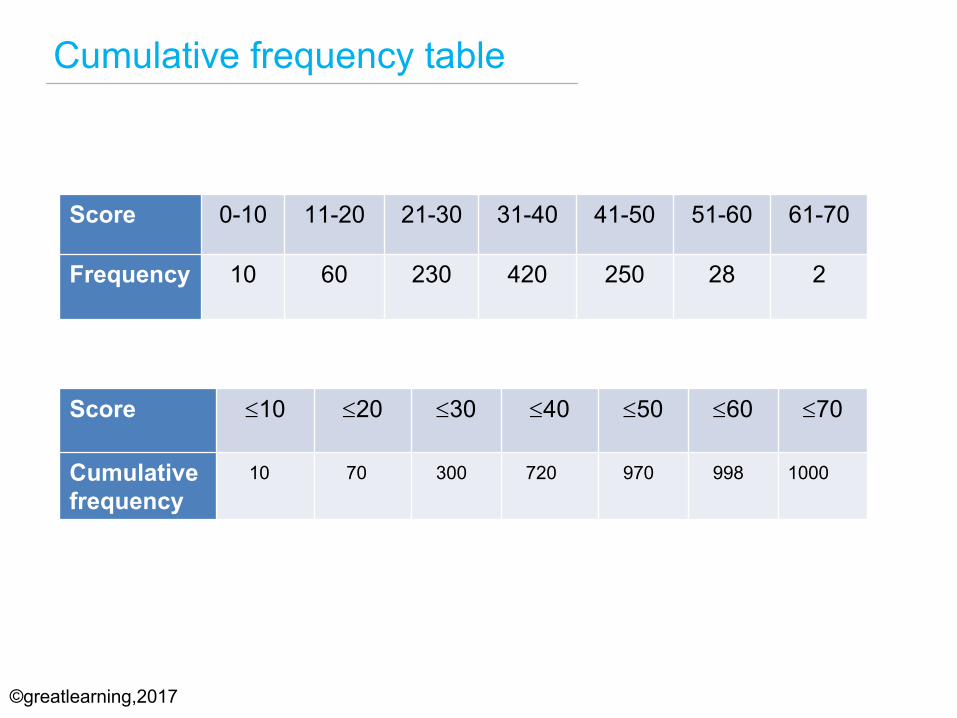
Cumulative frequency table
Score 0-10 11-20 21-30 31-40 41-50 51-60 61-70
Frequency 10 60 230 420 250 28 2
Score £10 £20 £30 £40 £50 £60 £70
Cumulative frequency
10 70 300 720 1000998970
©greatlearning,2017
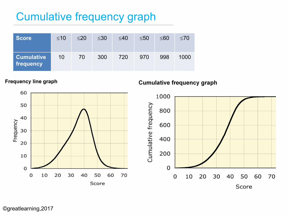
Cumulative frequency graph
Score £10 £20 £30 £40 £50 £60 £70
Cumulative frequency
10 70 300 720 970 998 1000
©greatlearning,2017
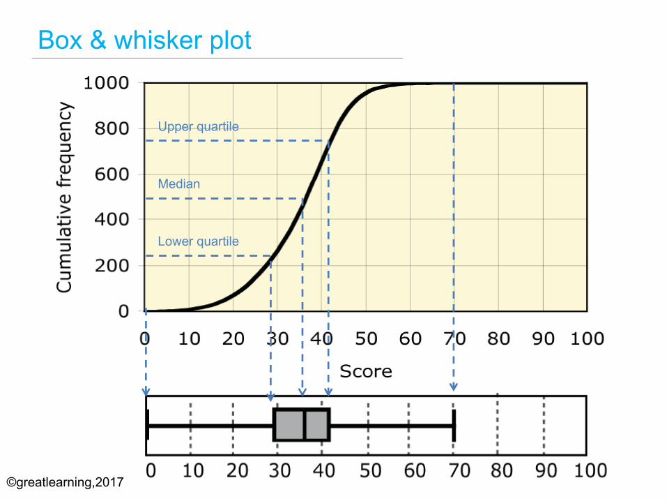
Box & whisker plot
Lower quartile
Upper quartile
Median
©greatlearning,2017
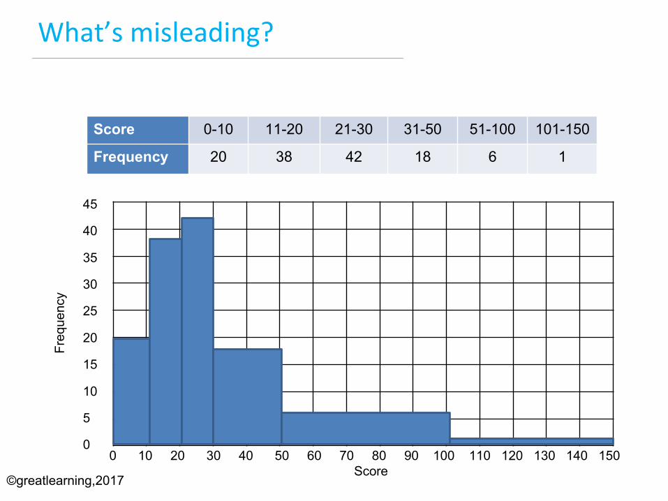
What’smisleading?
45
40
35
30
25
20
15
10
5
00 10 20 30 40 50 60 70 80 90 100 110 120 130 140 150
Score
Freq
uenc
y
Score 0-10 11-20 21-30 31-50 51-100 101-150
Frequency 20 38 42 18 6 1
©greatlearning,2017
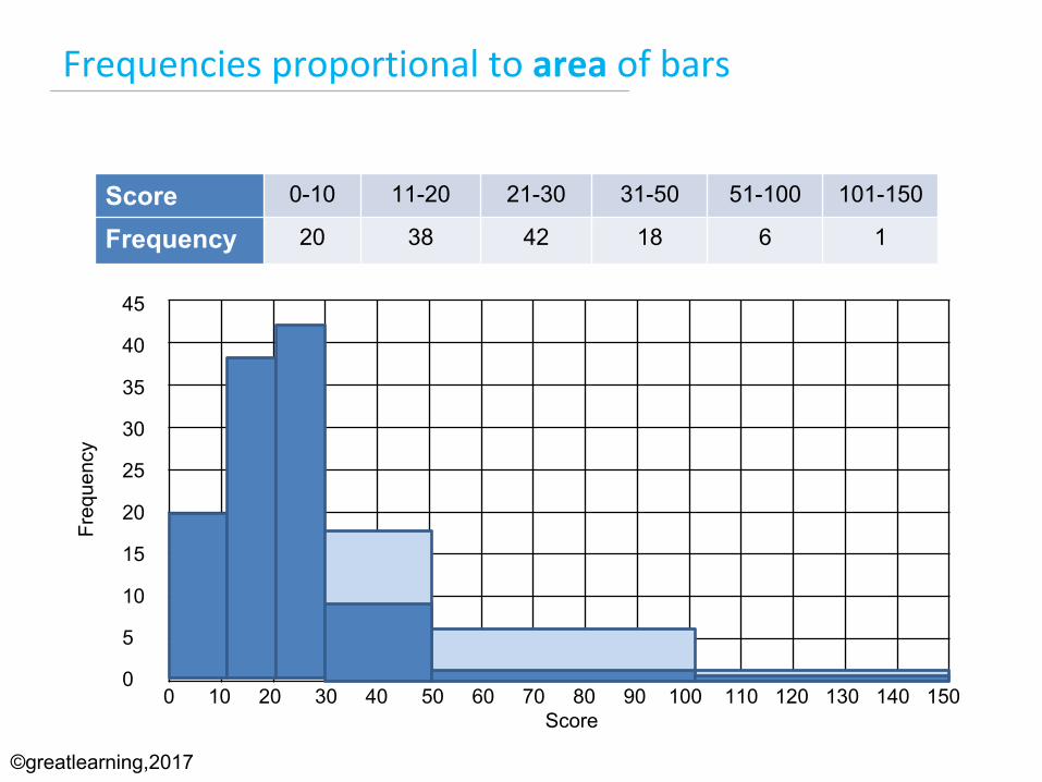
Frequenciesproportionaltoareaofbars
45
40
35
30
25
20
15
10
5
00 10 20 30 40 50 60 70 80 90 100 110 120 130 140 150
Score
Freq
uenc
y
Score 0-10 11-20 21-30 31-50 51-100 101-150
Frequency 20 38 42 18 6 1
©greatlearning,2017
Bivariate analysis
©greatlearning,2017
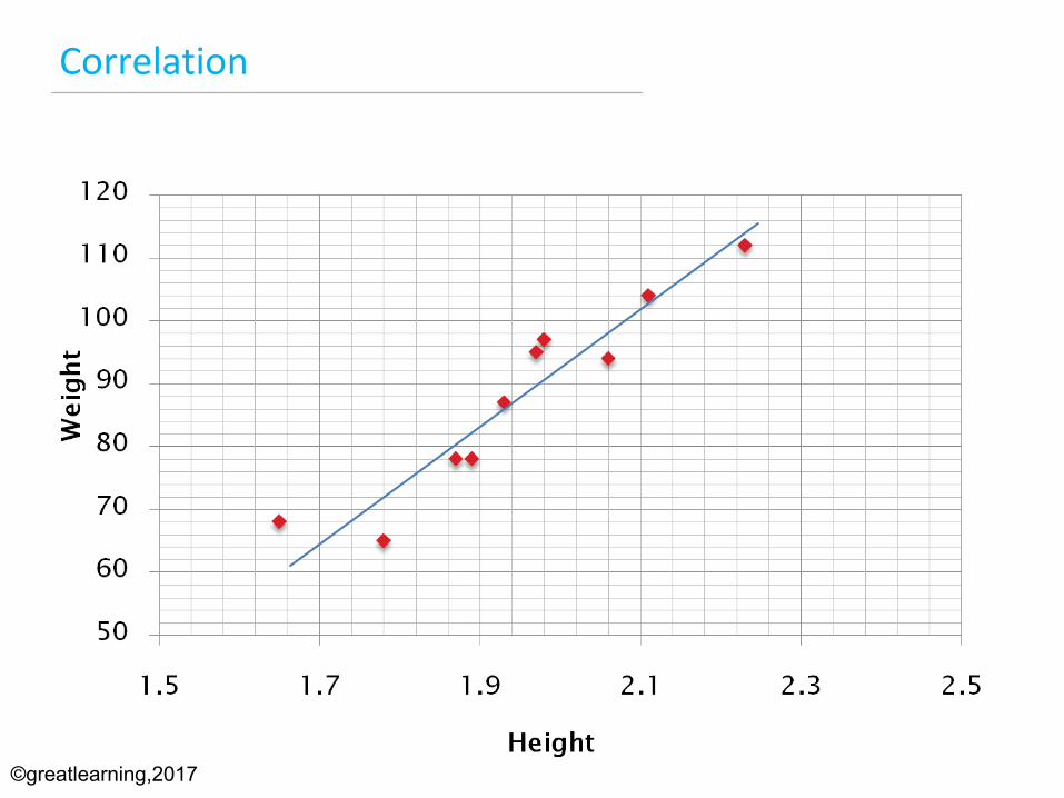
Correlation
©greatlearning,2017
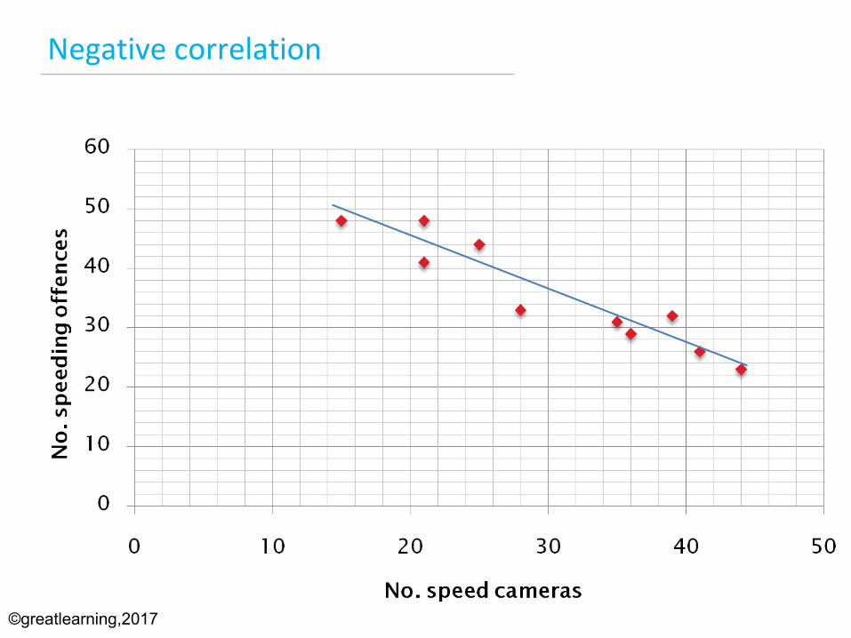
Negativecorrelation
©greatlearning,2017
Probability
©greatlearning,2017
Probability
P(a) = No. successful outcomesTotal possible outcomes
©greatlearning,2017
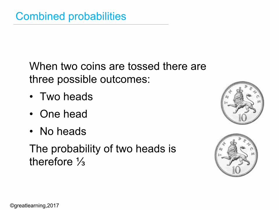
Combined probabilities
When two coins are tossed there are three possible outcomes: • Two heads• One head• No headsThe probability of two heads is therefore ⅓
©greatlearning,2017
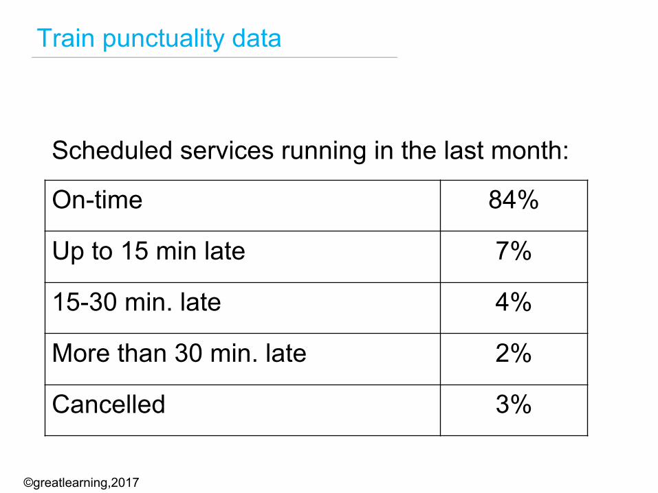
Train punctuality data
On-time 84%
Up to 15 min late 7%
15-30 min. late 4%
More than 30 min. late 2%
Cancelled 3%
Scheduled services running in the last month:
©greatlearning,2017
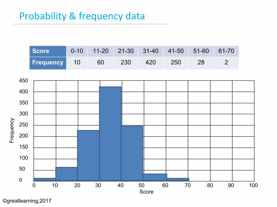
Probability&frequencydata
450
400
350
300
250
200
150
100
50
00 10 20 30 40 50 60 70 80 90 100
Score
Freq
uenc
y
Score 0-10 11-20 21-30 31-40 41-50 51-60 61-70
Frequency 10 60 230 420 250 28 2
©greatlearning,2017
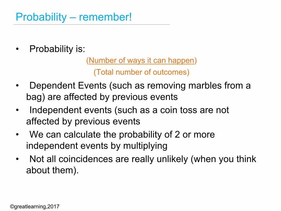
Probability – remember!
• Probability is: (Number of ways it can happen)
(Total number of outcomes)
• Dependent Events (such as removing marbles from a bag) are affected by previous events
• Independent events (such as a coin toss are not affected by previous events
• We can calculate the probability of 2 or more independent events by multiplying
• Not all coincidences are really unlikely (when you think about them).
©greatlearning,2017
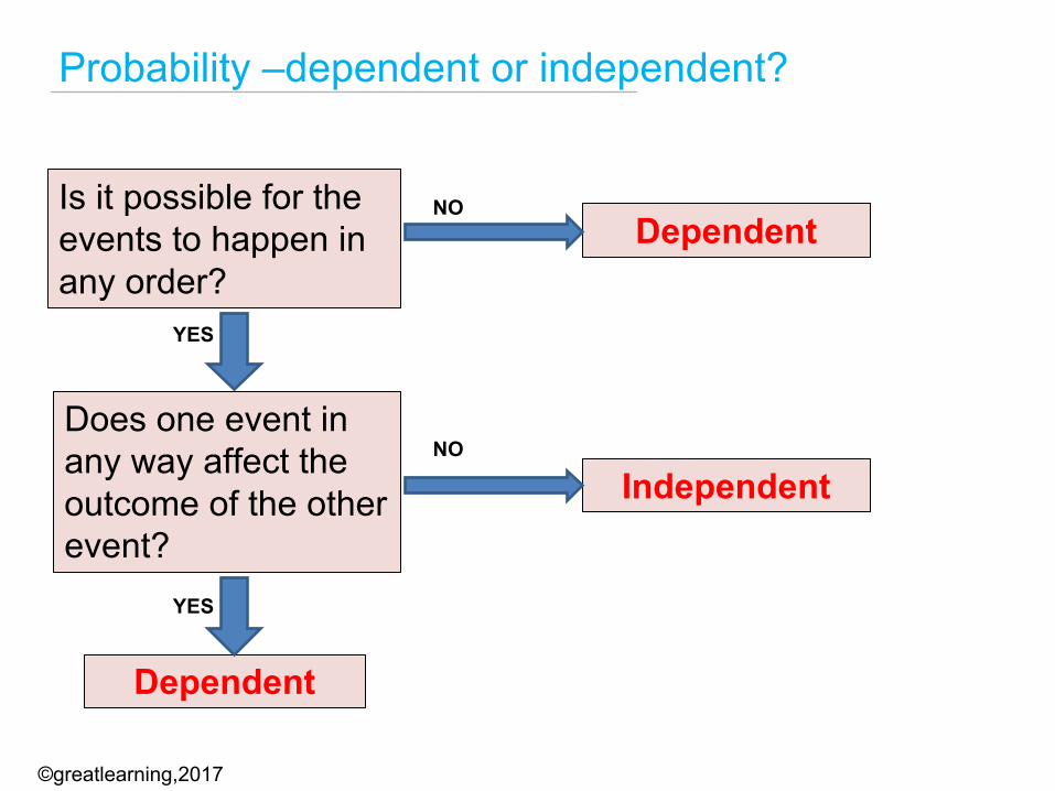
Probability –dependent or independent?
Is it possible for the events to happen in any order?
Does one event in any way affect the outcome of the other event?
Dependent
Dependent
Independent
YES
YES
NO
NO
©greatlearning,2017
Pearson’s correlation coefficient
©greatlearning,2017
The Pearson product-moment correlation coefficient (or Pearson correlation coefficient, for short)
is a measure of the strength of a linear association (the relationship) between two variables and is denoted by r. Basically, a Pearson product-moment correlation attempts to draw a line of best fit through the data of two variables, and the Pearson correlation coefficient, r, indicates how far away all these data points are to this line of best fit (i.e., how well the data points fit this new model/line of best fit).
©greatlearning,2017
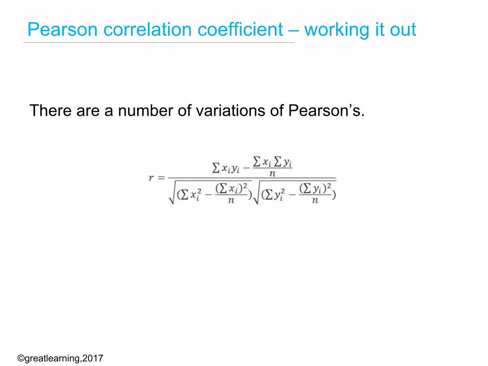
Pearson correlation coefficient – working it out
There are a number of variations of Pearson’s.
©greatlearning,2017
Pearson correlation coefficient cont
Pearson’s r is always between -1 and 1
©greatlearning,2017
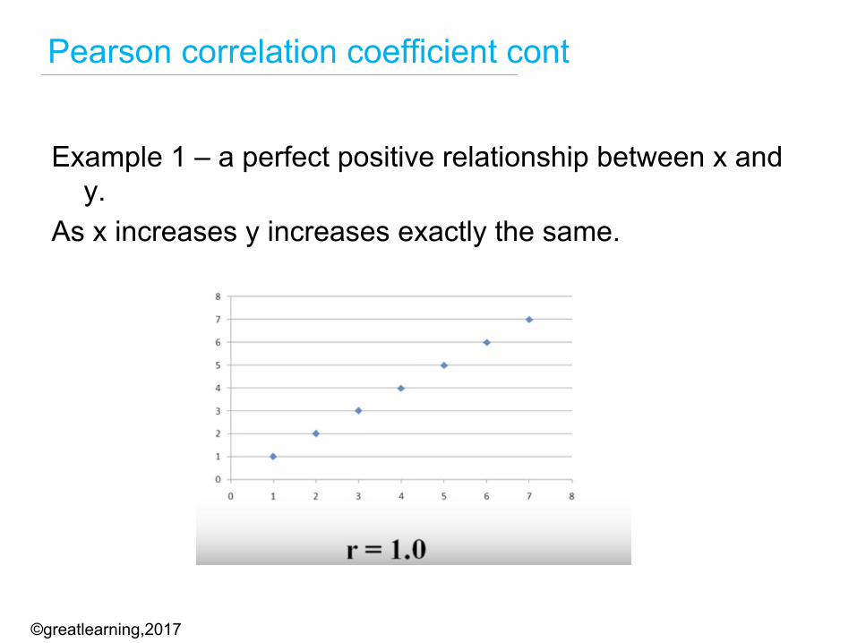
Pearson correlation coefficient cont
Example 1 – a perfect positive relationship between x and y.
As x increases y increases exactly the same.
©greatlearning,2017
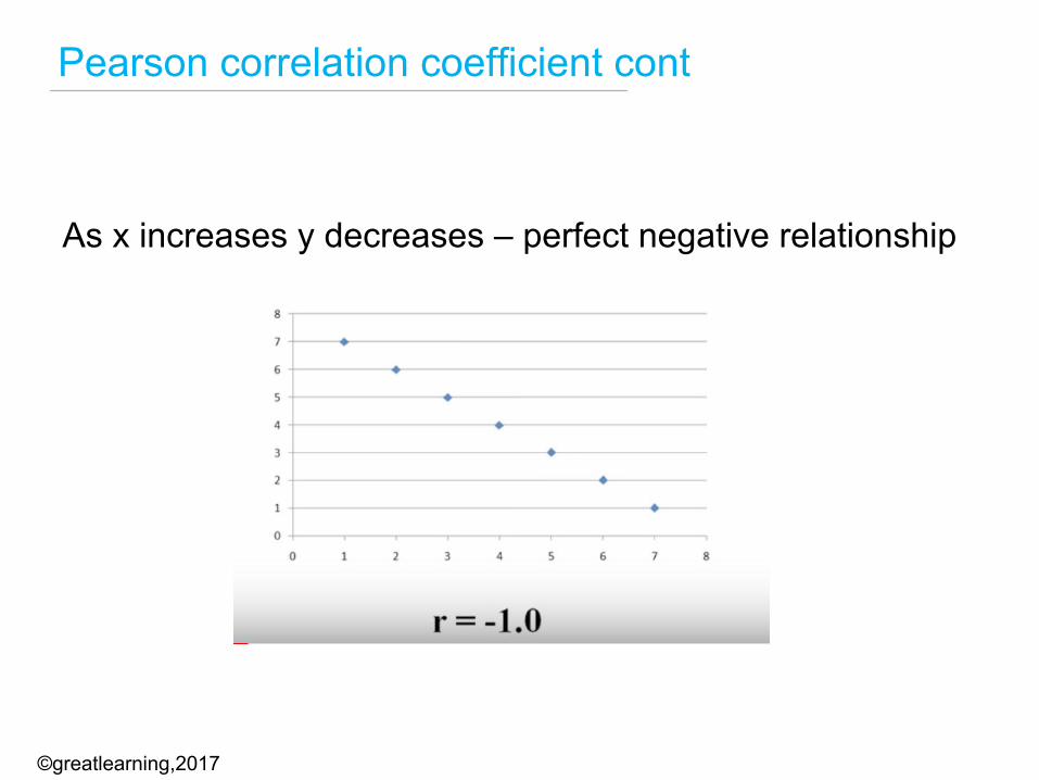
Pearson correlation coefficient cont
As x increases y decreases – perfect negative relationship
©greatlearning,2017
Pearson correlation coefficient cont
So what r=0 look like?
©greatlearning,2017
Pearson correlation coefficient cont
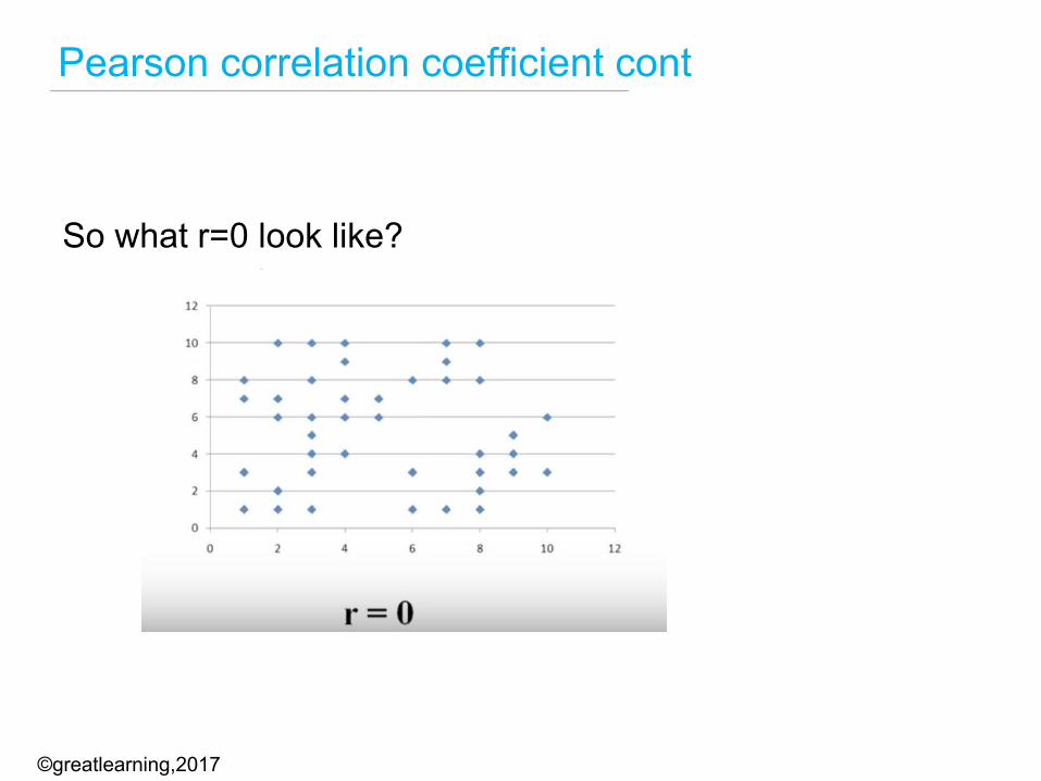
So what r=0 look like?
©greatlearning,2017
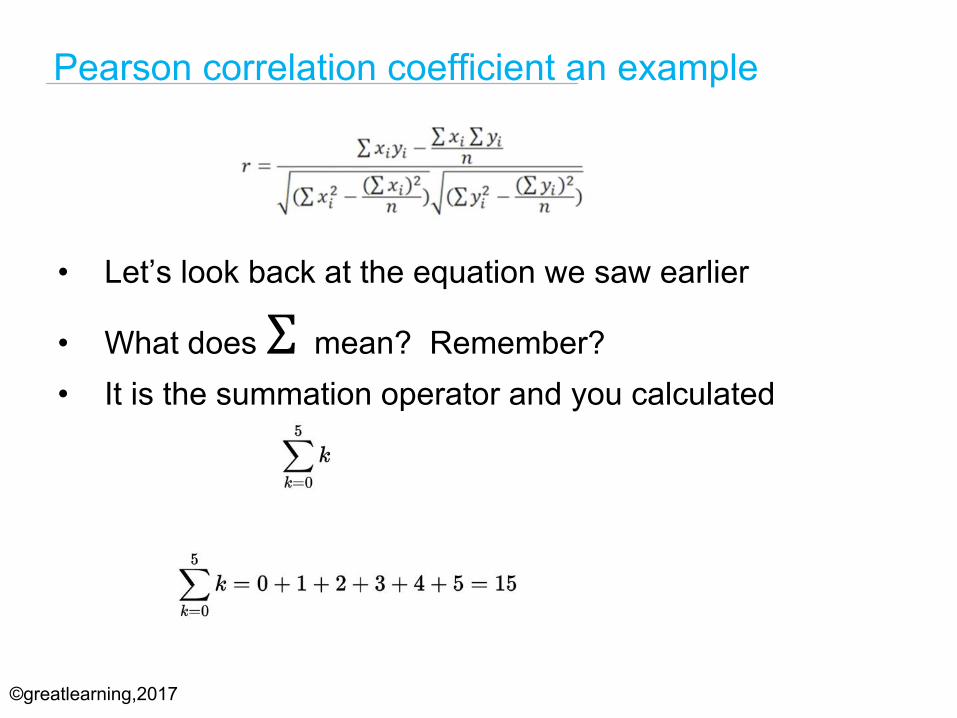
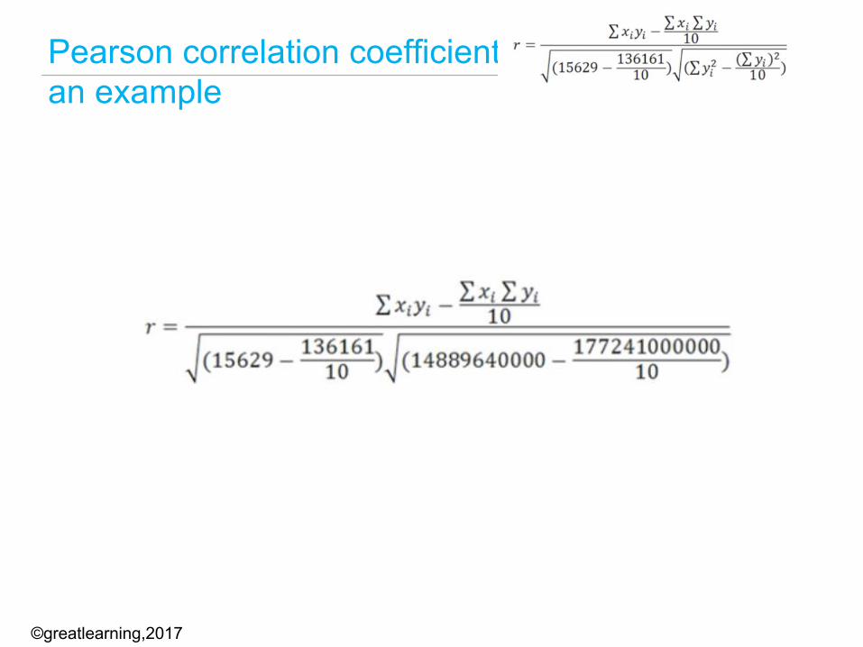
• Let’s look back at the equation we saw earlier
• What does Σ mean? Remember?• It is the summation operator and you calculated
Pearson correlation coefficient an example
©greatlearning,2017
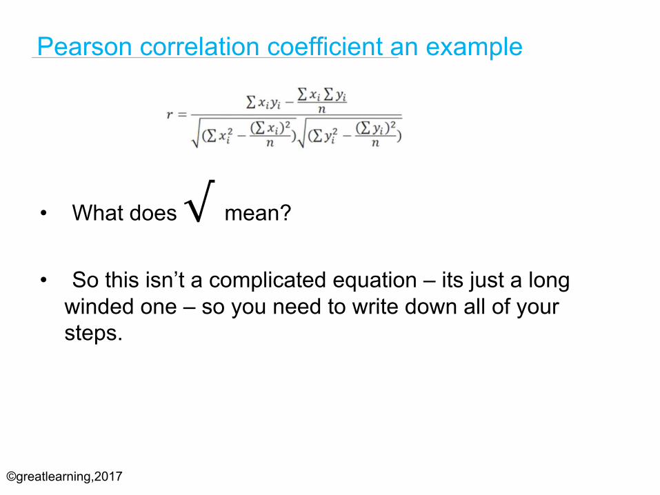
• What does √ mean?
• So this isn’t a complicated equation – its just a long winded one – so you need to write down all of your steps.
Pearson correlation coefficient an example
©greatlearning,2017
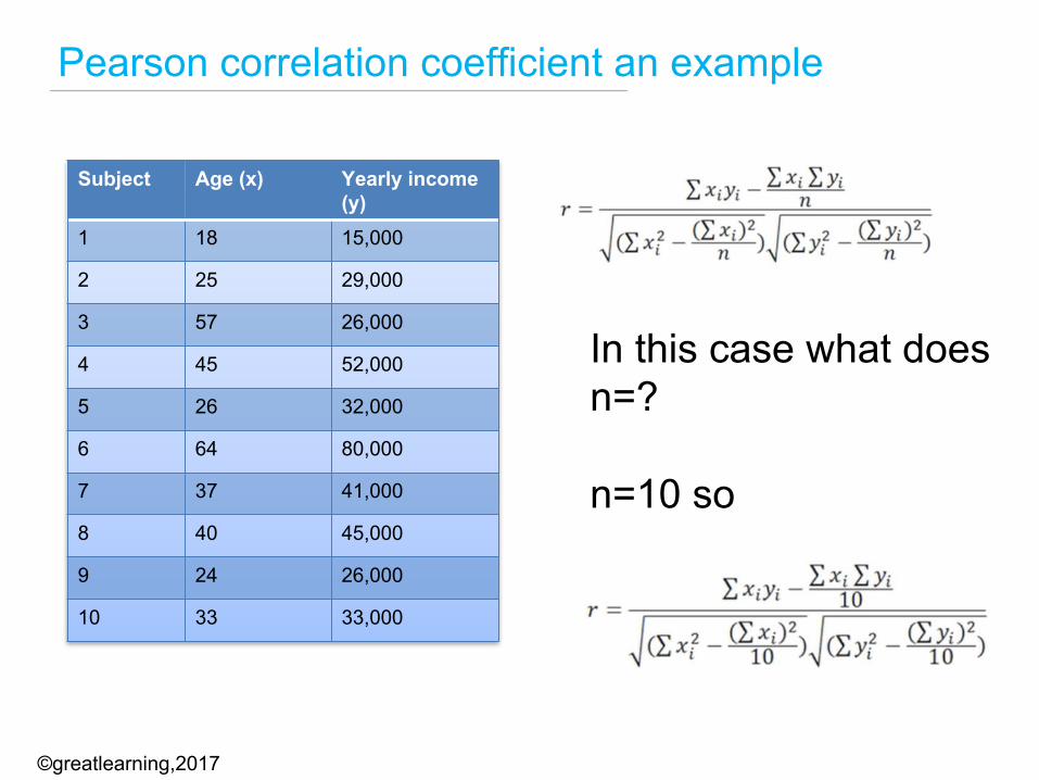
Pearson correlation coefficient an example
Subject Age (x) Yearly income (y)
1 18 15,000
2 25 29,000
3 57 26,000
4 45 52,000
5 26 32,000
6 64 80,000
7 37 41,000
8 40 45,000
9 24 26,000
10 33 33,000
In this case what does n=?
n=10 so
©greatlearning,2017
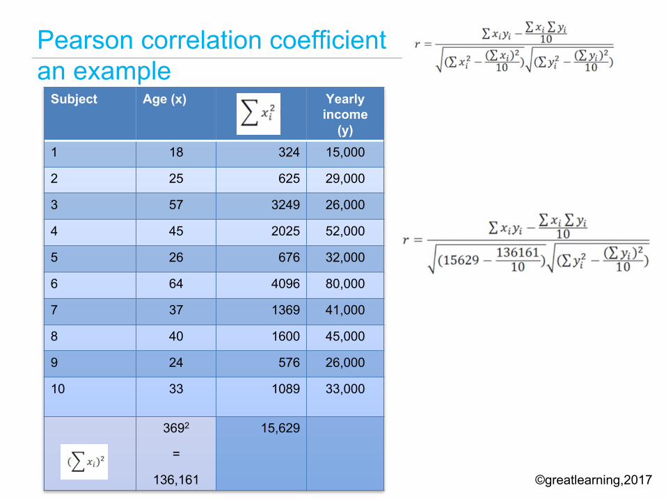
Pearson correlation coefficient an example
Subject Age (x) Yearly income
(y)1 18 324 15,000
2 25 625 29,000
3 57 3249 26,000
4 45 2025 52,000
5 26 676 32,000
6 64 4096 80,000
7 37 1369 41,000
8 40 1600 45,000
9 24 576 26,000
10 33 1089 33,000
3692
=
136,161
15,629
©greatlearning,2017
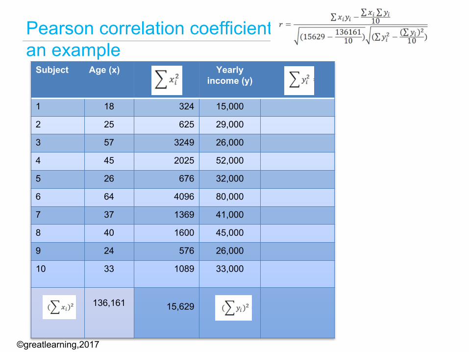
Pearson correlation coefficient an example
Subject Age (x) Yearly income (y)
1 18 324 15,000
2 25 625 29,000
3 57 3249 26,000
4 45 2025 52,000
5 26 676 32,000
6 64 4096 80,000
7 37 1369 41,000
8 40 1600 45,000
9 24 576 26,000
10 33 1089 33,000
136,161 15,629
©greatlearning,2017
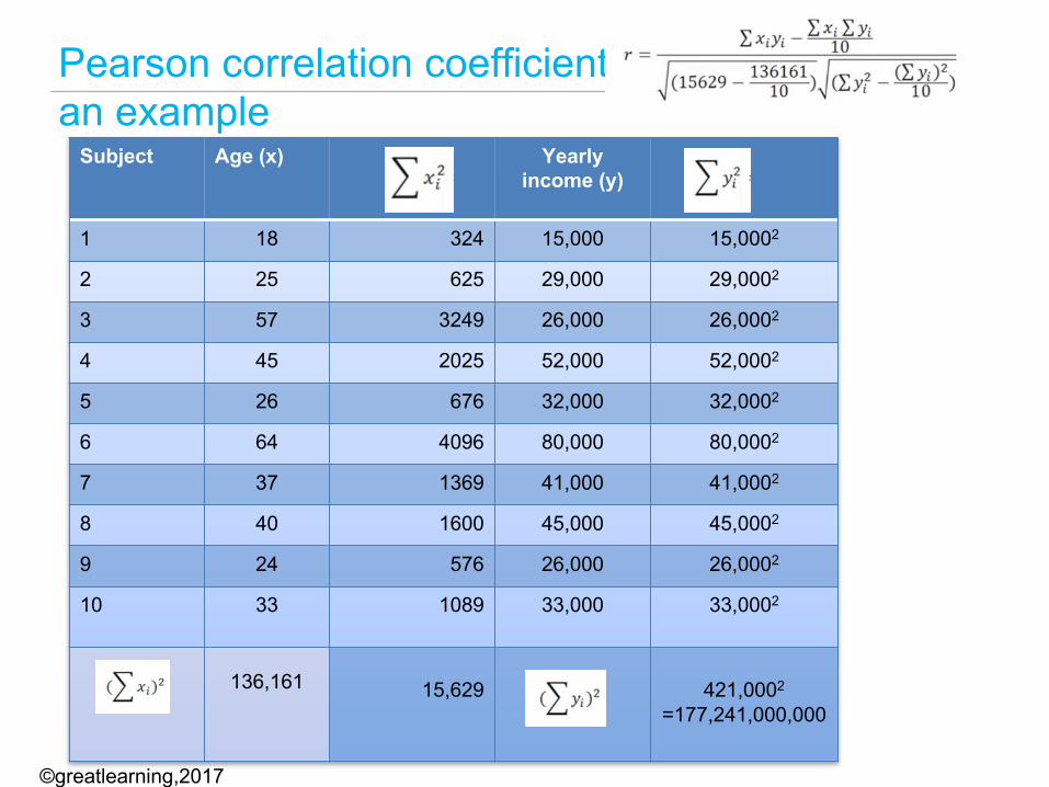
Pearson correlation coefficient an example
Subject Age (x) Yearly income (y)
1 18 324 15,000 15,0002
2 25 625 29,000 29,0002
3 57 3249 26,000 26,0002
4 45 2025 52,000 52,0002
5 26 676 32,000 32,0002
6 64 4096 80,000 80,0002
7 37 1369 41,000 41,0002
8 40 1600 45,000 45,0002
9 24 576 26,000 26,0002
10 33 1089 33,000 33,0002
136,161 15,629 421,0002
=177,241,000,000
©greatlearning,2017
Pearson correlation coefficient an example
©greatlearning,2017
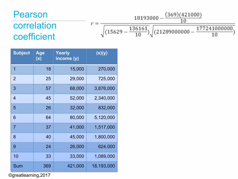
Pearson correlation coefficientSubject Age
(x)Yearly income (y)
(x)(y)
1 18 15,000 270,000
2 25 29,000 725,000
3 57 68,000 3,876,000
4 45 52,000 2,340,000
5 26 32,000 832,000
6 64 80,000 5,120,000
7 37 41,000 1,517,000
8 40 45,000 1,800,000
9 24 26,000 624,000
10 33 33,000 1,089,000
Sum 369 421,000 18,193,000
©greatlearning,2017
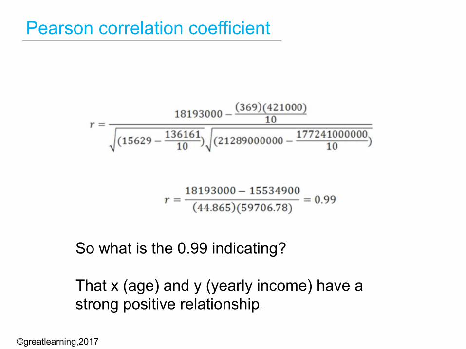
Pearson correlation coefficient
So what is the 0.99 indicating?
That x (age) and y (yearly income) have a strong positive relationship.
©greatlearning,2017
Pearson correlation coefficient cont
Pearson’s r is always between -1 and 1
https://statistics.laerd.com/statistical-guides/pearson-correlation-coefficient-statistical-guide.php
http://study.com/academy/lesson/pearson-correlation-coefficient-formula-example-significance.html
©greatlearning,2017
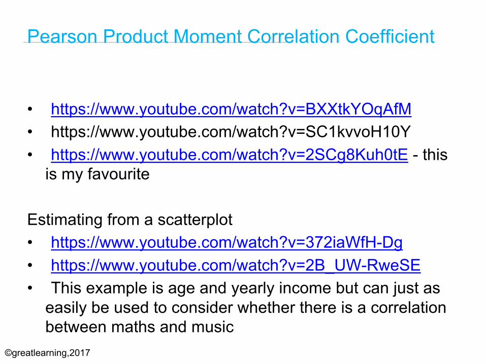
• https://www.youtube.com/watch?v=BXXtkYOqAfM• https://www.youtube.com/watch?v=SC1kvvoH10Y• https://www.youtube.com/watch?v=2SCg8Kuh0tE - this
is my favourite
Estimating from a scatterplot• https://www.youtube.com/watch?v=372iaWfH-Dg• https://www.youtube.com/watch?v=2B_UW-RweSE• This example is age and yearly income but can just as
easily be used to consider whether there is a correlation between maths and music
Pearson Product Moment Correlation Coefficient
©greatlearning,2017
Questions for you to work on:
• Probability• Statistics• Statistical distributions• Correlation and regression
©greatlearning,2017
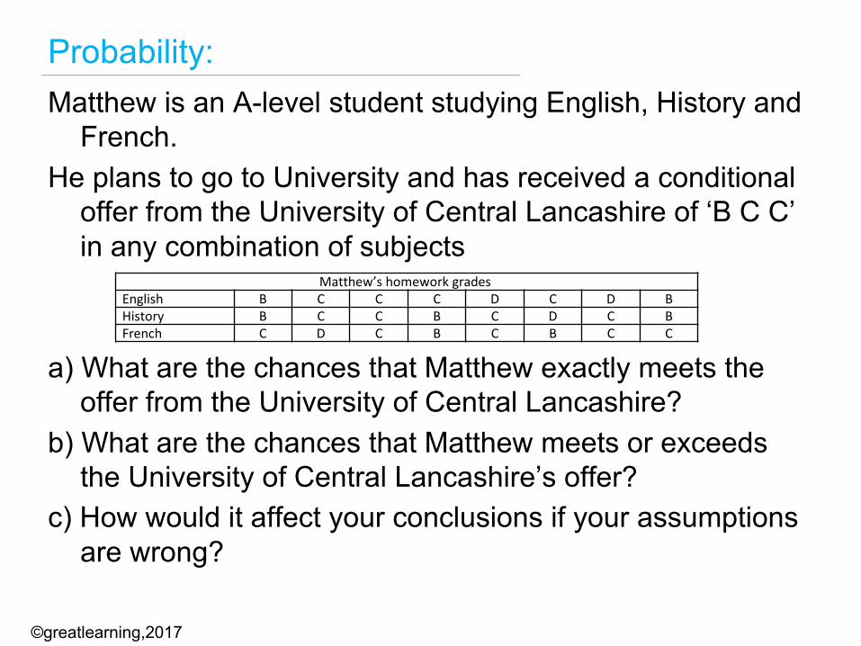
Probability:Matthew is an A-level student studying English, History and
French.He plans to go to University and has received a conditional
offer from the University of Central Lancashire of ‘B C C’ in any combination of subjects
a) What are the chances that Matthew exactly meets the offer from the University of Central Lancashire?
b) What are the chances that Matthew meets or exceeds the University of Central Lancashire’s offer?
c) How would it affect your conclusions if your assumptions are wrong?
Matthew’shomeworkgradesEnglish B C C C D C D BHistory B C C B C D C BFrench C D C B C B C C
©greatlearning,2017
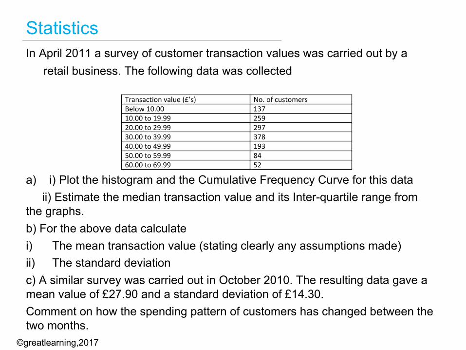
StatisticsIn April 2011 a survey of customer transaction values was carried out by a
retail business. The following data was collected
a) i) Plot the histogram and the Cumulative Frequency Curve for this dataii) Estimate the median transaction value and its Inter-quartile range from
the graphs.b) For the above data calculatei) The mean transaction value (stating clearly any assumptions made)ii) The standard deviationc) A similar survey was carried out in October 2010. The resulting data gave a mean value of £27.90 and a standard deviation of £14.30.Comment on how the spending pattern of customers has changed between the two months.
Transactionvalue(£’s) No.ofcustomersBelow10.00 13710.00to19.99 25920.00to29.99 29730.00to39.99 37840.00to49.99 19350.00to59.99 8460.00to69.99 52
©greatlearning,2017
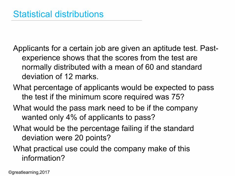
Statistical distributions
Applicants for a certain job are given an aptitude test. Past-experience shows that the scores from the test are normally distributed with a mean of 60 and standard deviation of 12 marks.
What percentage of applicants would be expected to pass the test if the minimum score required was 75?
What would the pass mark need to be if the company wanted only 4% of applicants to pass?
What would be the percentage failing if the standard deviation were 20 points?
What practical use could the company make of this information?
©greatlearning,2017
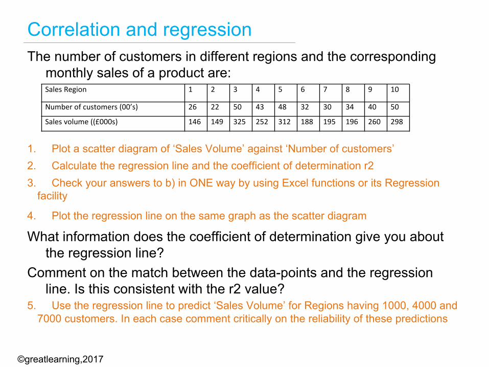
Correlation and regressionThe number of customers in different regions and the corresponding
monthly sales of a product are:
1. Plot a scatter diagram of ‘Sales Volume’ against ‘Number of customers’2. Calculate the regression line and the coefficient of determination r23. Check your answers to b) in ONE way by using Excel functions or its Regression
facility
4. Plot the regression line on the same graph as the scatter diagram
What information does the coefficient of determination give you about the regression line?
Comment on the match between the data-points and the regression line. Is this consistent with the r2 value?
5. Use the regression line to predict ‘Sales Volume’ for Regions having 1000, 4000 and 7000 customers. In each case comment critically on the reliability of these predictions
SalesRegion 1 2 3 4 5 6 7 8 9 10
Numberofcustomers(00’s) 26 22 50 43 48 32 30 34 40 50
Salesvolume((£000s) 146 149 325 252 312 188 195 196 260 298
©greatlearning,2017

![GRUNDFOS ALPHA+net.grundfos.com/Appl/ccmsservices/public/... · Uputstvo za montažu i upotrebu 170 ... uct GRUNDFOS ALPHA+, to which this declaration relates, is in ... [°C] Liquid](https://static.fdocument.org/doc/165x107/5e50725de29b1a0feb3efab8/grundfos-alphanet-uputstvo-za-montau-i-upotrebu-170-uct-grundfos-alpha.jpg)