Superconducting qubits

Sergey N. Shevchenko

B. Verkin Institute for Low Temperature Physics and Engineering, Kharkov

Summer School on Modern Quantum Technologies, BITP, Kiev

September 14th 2018

Φ

Now we have to have: (1) Lecture

(2) Tutorials

We will not consider these separately. We will now rather have the superposition of (1) and (2), in the spirit of Newton’s “When studying science, the examples are more useful than the rules”.

• Current-biased junction => phase qubit • Superconducting island => charge qubit • Ring with junctions => flux qubit

• and dynamic phenomena in (superconducting) qubits:

Landau-Zener-Stückelberg-Majorana and multi-photon transitions

AGENDA

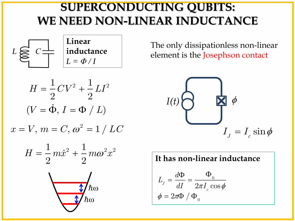
Linear inductance L = Φ / I

SUPERCONDUCTING QUBITS: WE NEED NON-LINEAR INDUCTANCE

ℏω

ℏω

It has non-linear inductance

The only dissipationless non-linear element is the Josephson contact L С

sinJ cI I

0

0

2 cos2 /

Jc

dL

dI I

2 21 1

2 2H CV LI

I(t) ( , / )V I L

2, , 1/x V m C LC

2 2 21 1

2 2H mx m x

JOSEPHSON EFFECT – summary

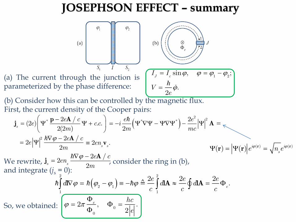
(a) The current through the junction is parameterized by the phase difference:

(b) Consider how this can be controlled by the magnetic flux. First, the current density of the Cooper pairs:

* 2 /(2 ) . .

2(2 )s

e ce cc

m

p Aj

22* * 2

2

e eim mc

A

2 .s sen v

2 2 /2

2

e ce

m

A ( ) ( )( ) ( ) i i

se n er rr r

2 /2

2s s

e cen

m

AjWe rewrite, , consider the ring in (b),

and integrate (js = 0):

2 2

2 11 1

2 2 2.e

e e ed d d

c c cl lA lA

So, we obtained:

00

2 , .2

e hc

e

1 2sin , ;

.2

J cI I

Ve

JOSEPHSON EFFECT – summary

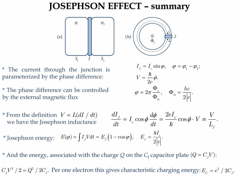
* The current through the junction is parameterized by the phase difference:

* The phase difference can be controlled by the external magnetic flux

00

2 , .2

e hc

e

1 2sin , ;

.2

J cI I

Ve

* From the definition we have the Josephson inductance

( / )V L dI dt

2cos cos .J cc

J

dI eId VI V

dt dt L

* Josephson energy: ( ) 1 cos , .2c

J J J

IE I Vdt E E

e

* And the energy, associated with the charge Q on the CJ capacitor plate : ( )J

Q C V

2 2/ 2 / 2 .J JC V Q C Per one electron this gives characteristic charging energy: 2 / 2 .

C JE e C

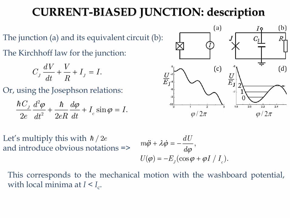
CURRENT-BIASED JUNCTION: description

.J J

dV VC I Idt R

The junction (a) and its equivalent circuit (b):

The Kirchhoff law for the junction:

2

2sin .

2 2J

c

C d dI I

e eR dtdt

Or, using the Josephson relations:

Let’s multiply this with and introduce obvious notations =>

/ 2e

,

( ) (cos / ).J c

dUm

dU E I I

This corresponds to the mechanical motion with the washboard potential, with local minima at I < Ic.

CURRENT-BIASED JUNCTION: Lagrangian

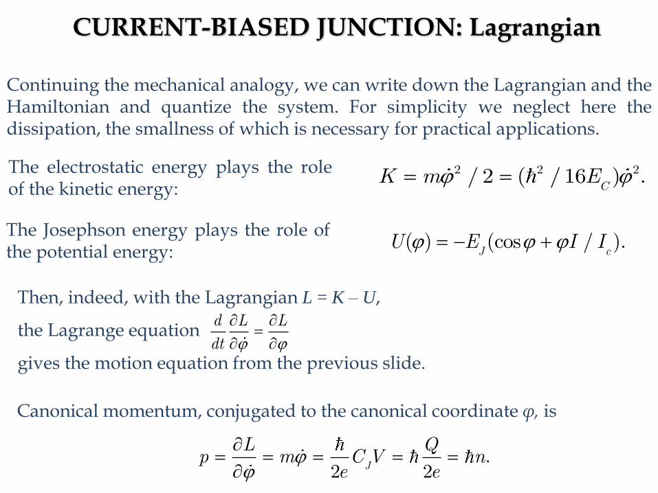
Continuing the mechanical analogy, we can write down the Lagrangian and the Hamiltonian and quantize the system. For simplicity we neglect here the dissipation, the smallness of which is necessary for practical applications.

2 2 2/ 2 ( /16 ) .C

K m EThe electrostatic energy plays the role of the kinetic energy:

The Josephson energy plays the role of the potential energy:

( ) (cos / ).J c

U E I I

Then, indeed, with the Lagrangian L = K – U,

the Lagrange equation

gives the motion equation from the previous slide.

d L L

dt

Canonical momentum, conjugated to the canonical coordinate φ, is

.2 2J

L Qp m C V n

e e

CURRENT-BIASED JUNCTION: quantization

( , )H p p L

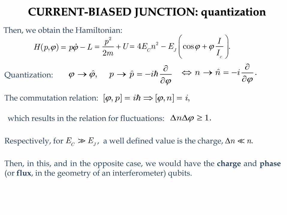
Then, we obtain the Hamiltonian:

24 cos .C J

c

IE n E

I

2

2

pU

m

Quantization:

ˆ ˆ, p p i

ˆ .n n i

The commutation relation: [ , ] [ , ] ,p i n i

which results in the relation for fluctuations: 1.n

Respectively, for , a well defined value is the charge, C JE E .n n

Then, in this, and in the opposite case, we would have the charge and phase (or flux, in the geometry of an interferometer) qubits.

CURRENT-BIASED JUNCTION => phase qubit

The quantization results in the appearance of discrete energy levels in the potential with local minima. Importantly, with non-equidistant levels. For the description of the phase qubit, we approximate the potential U by a parabola, expanding it near the minimum, where

0 (sin / )J c

U E I I 0arcsin / .

cI I

2 220 0

0

2

2 02

( ) ( )cos ,

2 2

cos 81 .

J q

J J Cq

c

U E m

E E E I

m I

( 1/ 2).k qE k

1 0

.q

E E E

Then, omitting the constant term, we have

The energy levels in such harmonic potential:

So, the distance between the qubit energy levels: And this is defined by the bias current, ( ).

q qI

PHASE QUBIT: operation

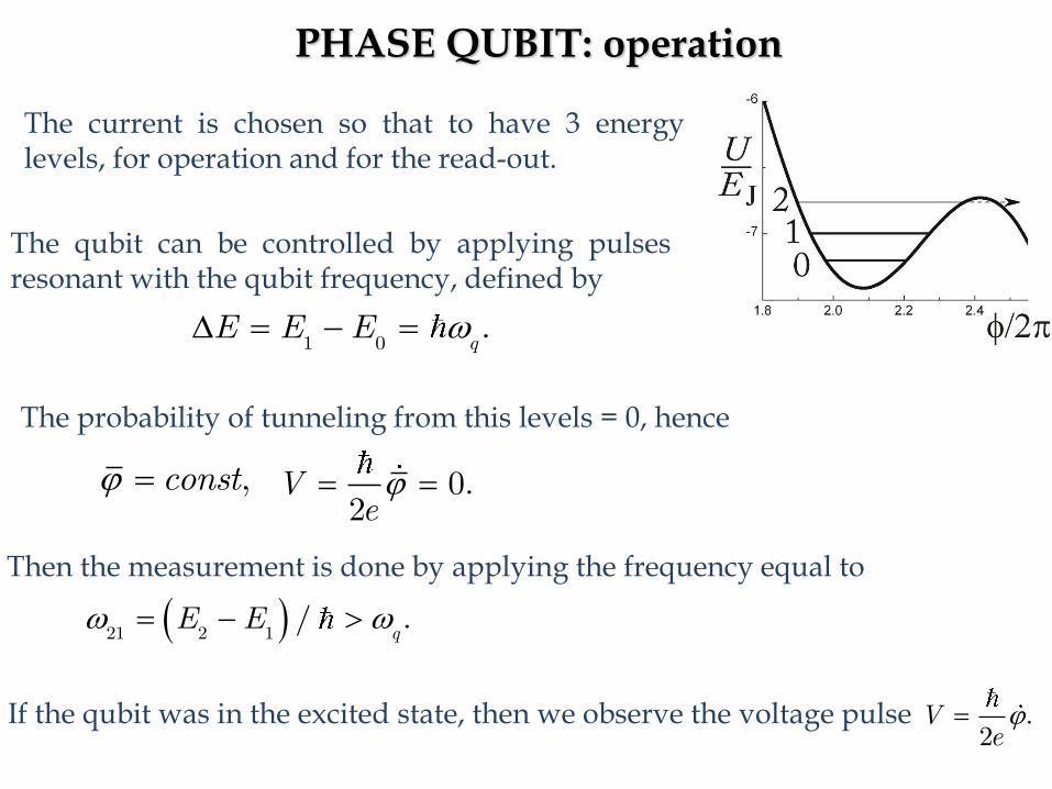
The qubit can be controlled by applying pulses resonant with the qubit frequency, defined by

1 0

.q

E E E

,const 0.2

Ve

21 2 1

/ .q

E E

Then the measurement is done by applying the frequency equal to

.2

Ve

The current is chosen so that to have 3 energy levels, for operation and for the read-out.

The probability of tunneling from this levels = 0, hence

If the qubit was in the excited state, then we observe the voltage pulse

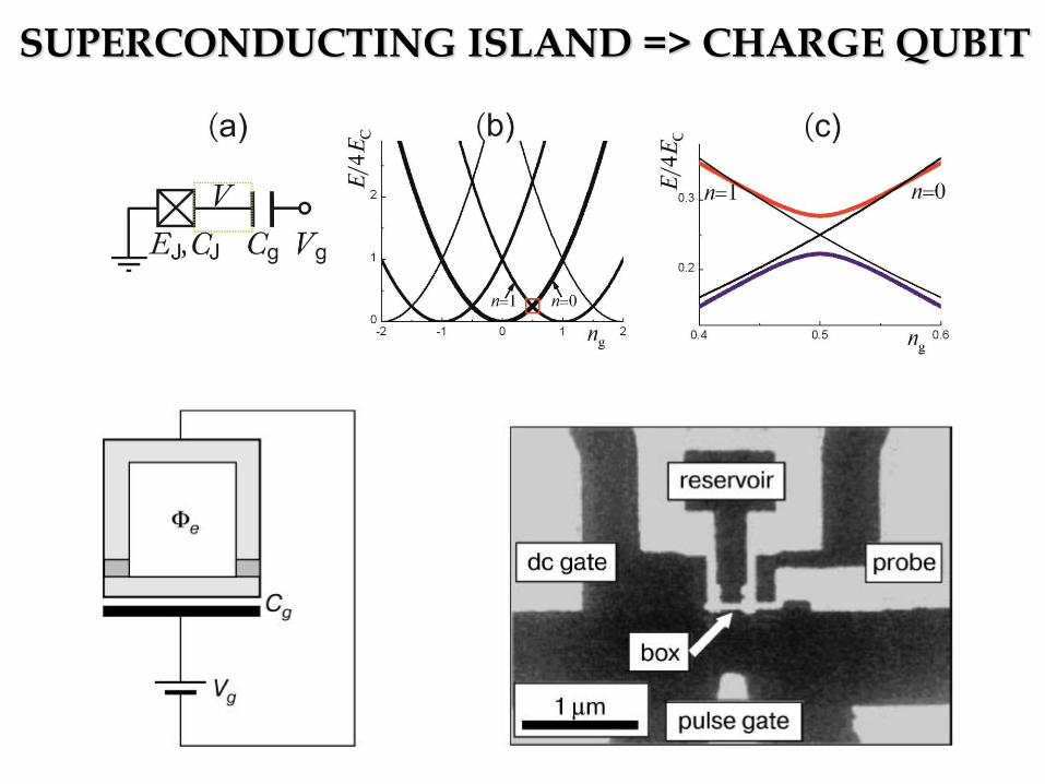
SUPERCONDUCTING ISLAND => CHARGE QUBIT

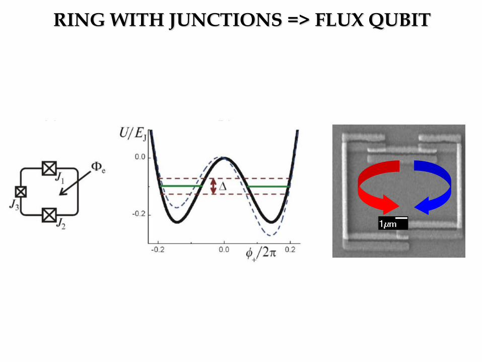
RING WITH JUNCTIONS => FLUX QUBIT

How to excite qubits?

We need the resonant pulse: .E h

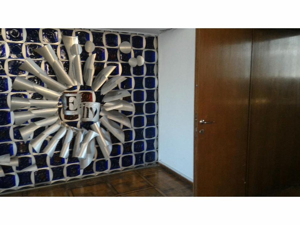
reCAPTCHA?

No. It is one of the nice artistic objects here.

See there

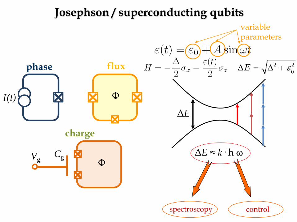
phase flux

spectroscopy

ΔE

Φ

ΔE ≈ k· ħ ω

2 2

0E

variable parameters

I(t)

charge

Φ Vg

Cg

control

Josephson / superconducting qubits

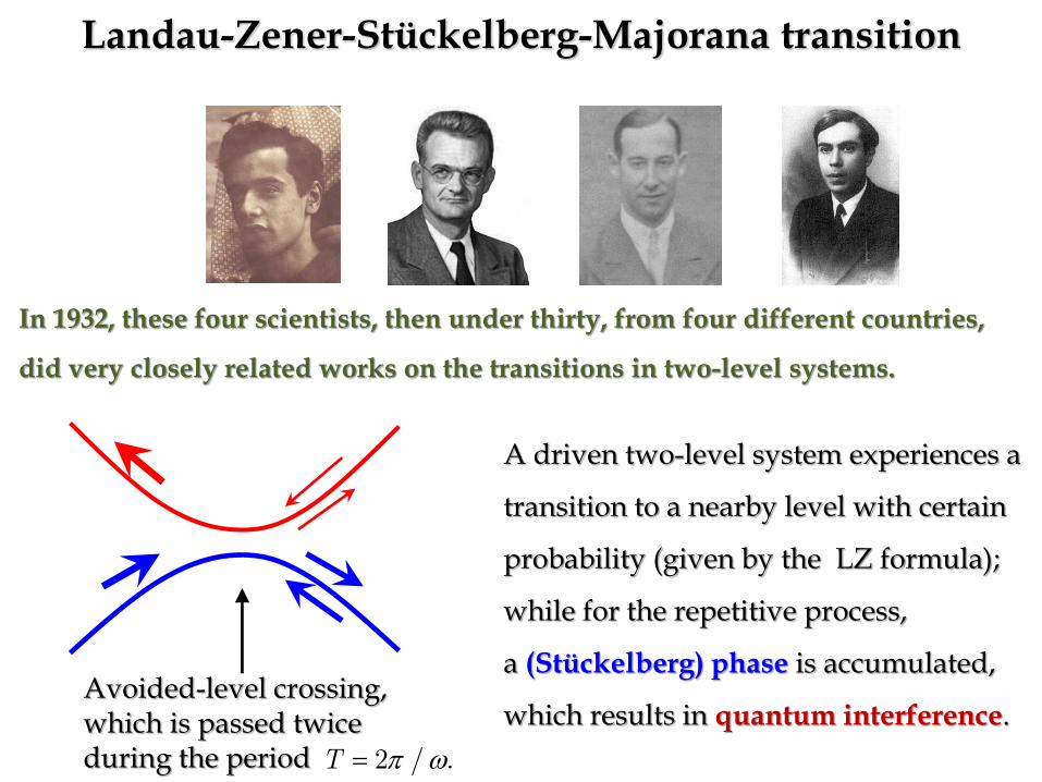
A driven two-level system experiences a

transition to a nearby level with certain

probability (given by the LZ formula);

while for the repetitive process,

a (Stückelberg) phase is accumulated,

which results in quantum interference.

In 1932, these four scientists, then under thirty, from four different countries,

did very closely related works on the transitions in two-level systems.

Avoided-level crossing, which is passed twice during the period 2 / .T

Landau-Zener-Stückelberg-Majorana transition

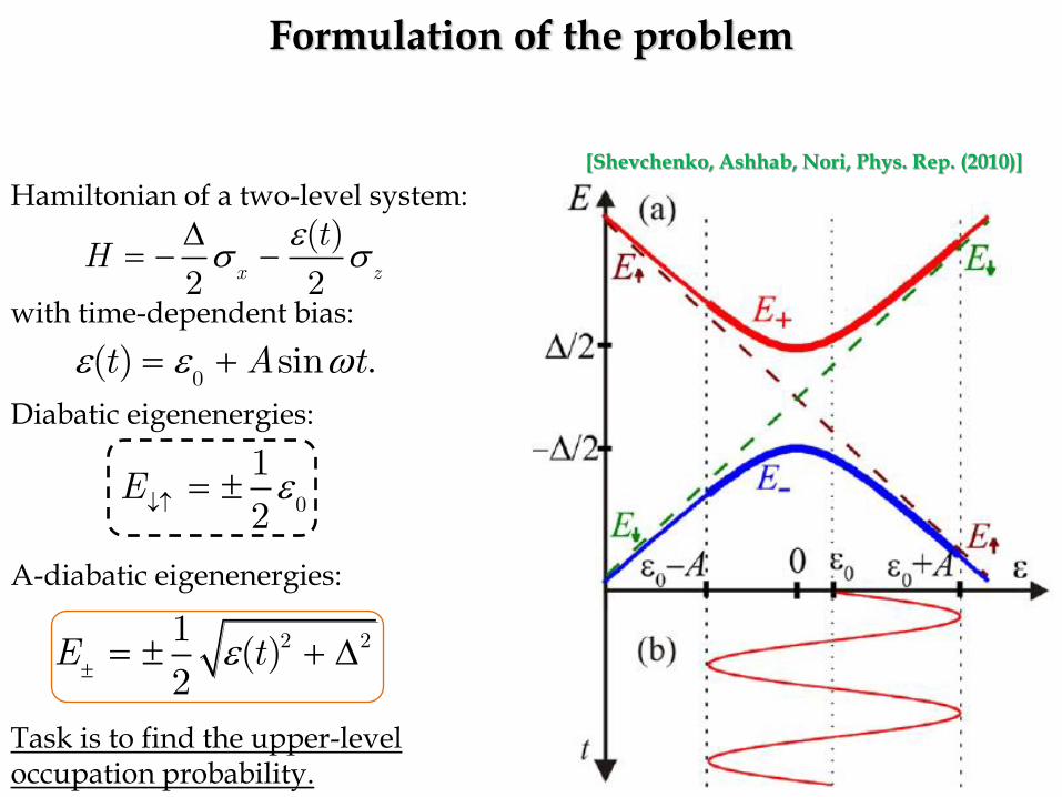
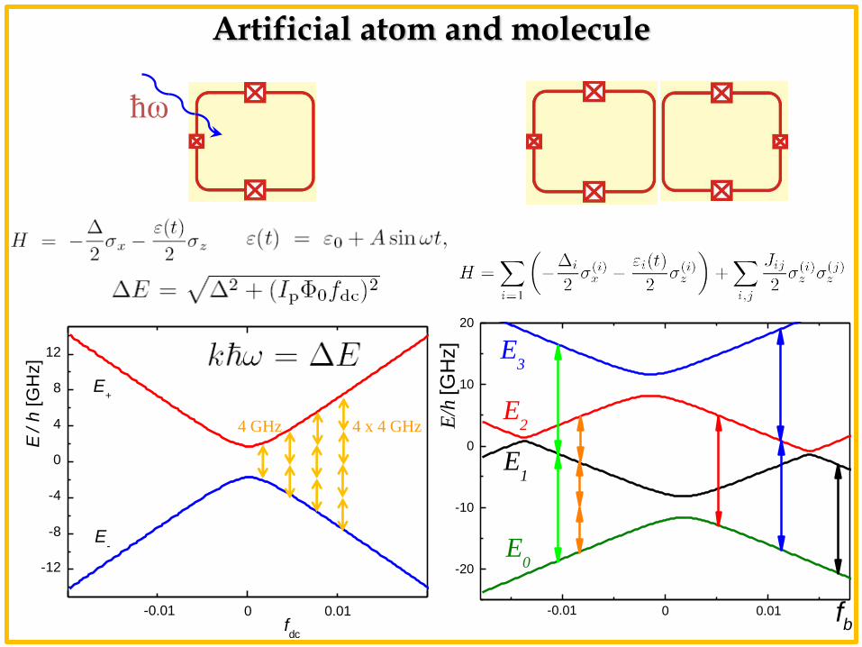
Hamiltonian of a two-level system:

with time-dependent bias:

Diabatic eigenenergies:

0

1

2E

A-diabatic eigenenergies:

2 21( )

2E t

( )

2 2x z

tH

0( ) sin .t A t

Task is to find the upper-level occupation probability.

[Shevchenko, Ashhab, Nori, Phys. Rep. (2010)]

Formulation of the problem

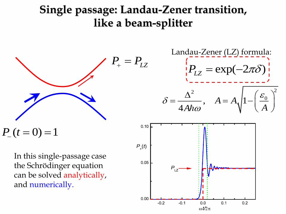
( 0) 1 P t

LZP Pexp( 2 ) LZP

22

0, 14

A A

AA

In this single-passage case the Schrödinger equation can be solved analytically, and numerically.

Landau-Zener (LZ) formula:

Single passage: Landau-Zener transition, like a beam-splitter

2

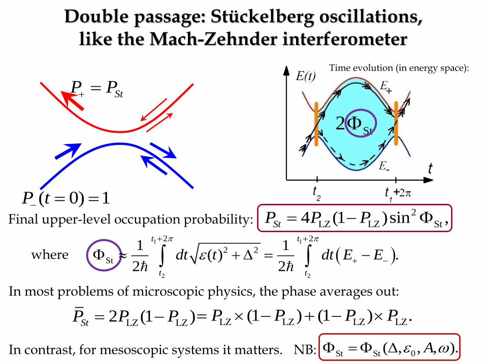
LZ LZ St4 (1 )sin , StP P P

( 0) 1 P t

StP P

St2

Time evolution (in energy space):

Final upper-level occupation probability:

In most problems of microscopic physics, the phase averages out:

LZ LZ2 (1 ) StP P P

In contrast, for mesoscopic systems it matters.

1 1

2 2

2 2

2 2

St

1 1( ) .

2 2

t t

t t

dt t dt E Ewhere

LZ LZ LZ LZ(1 ) (1 ) . P P P P

NB: St St 0( , , , ). A

Double passage: Stückelberg oscillations, like the Mach-Zehnder interferometer

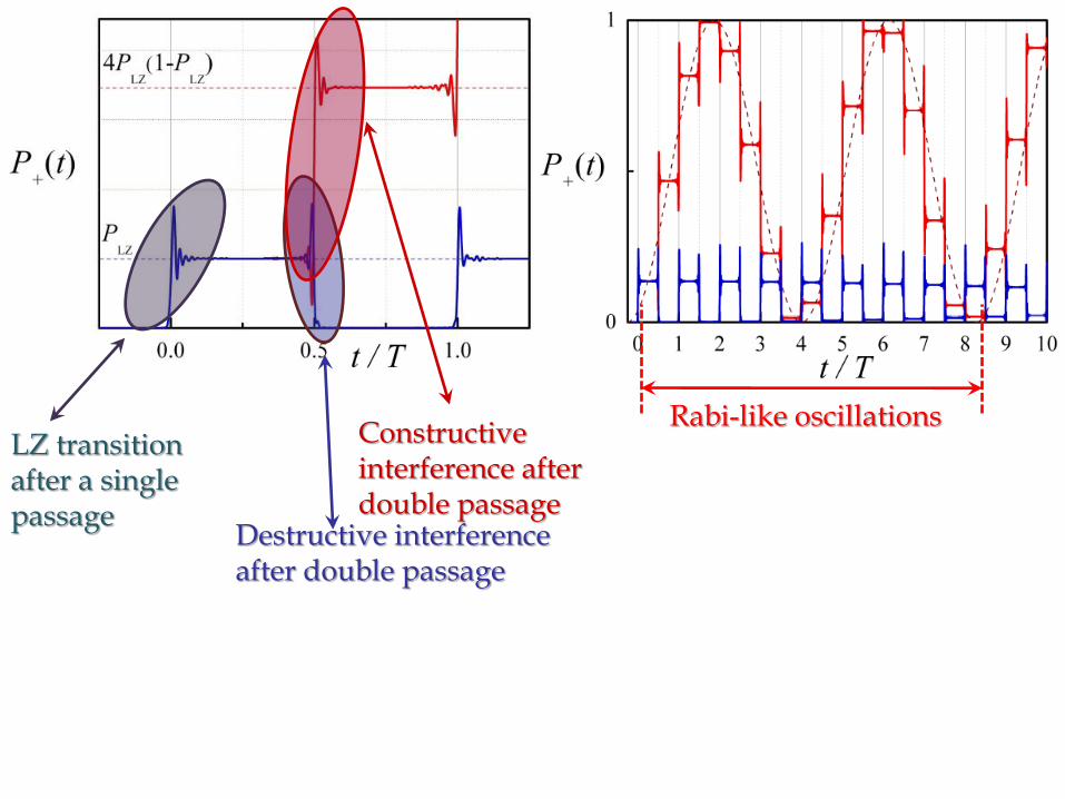
LZ transition after a single passage

Destructive interference after double passage

Constructive interference after double passage

Rabi-like oscillations

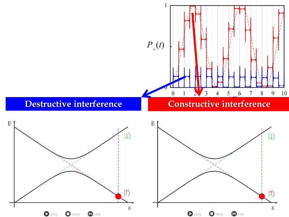
Destructive interference Constructive interference

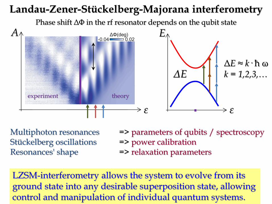
Phase shift ΔΦ in the rf resonator depends on the qubit state

Multiphoton resonances => parameters of qubits / spectroscopy Stückelberg oscillations => power calibration Resonances' shape => relaxation parameters

theory experiment

ε

A

ε

E

LZSM-interferometry allows the system to evolve from its ground state into any desirable superposition state, allowing control and manipulation of individual quantum systems.

ΔE ≈ k· ħ ω k = 1,2,3,… ΔE

Landau-Zener-Stückelberg-Majorana interferometry

23

Systems of coupled superconducting qubits can be realized, probed and controlled.

Micrograph (top) and scheme (right)

Example: excitation of a two-qubit system

-12

-8

-4

0

4

8

12

-0.01 0.01

E-

E+

0

E /

h [

GH

z]

fdc

4 x 4 GHz 4 GHz

-20

-10

0

10

20

0.010-0.01

E3

E2

E1

E0

E/h

[G

Hz]

fb

ħω

Artificial atom and molecule

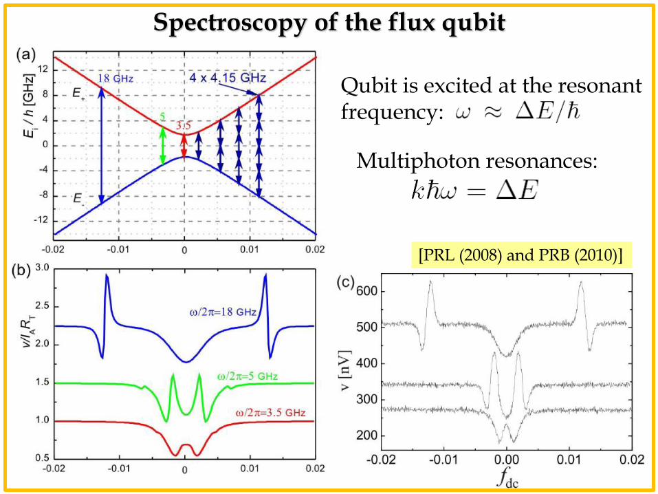
Qubit is excited at the resonant frequency:

Multiphoton resonances:

[PRL (2008) and PRB (2010)]

Spectroscopy of the flux qubit

-20

-10

0

10

20

0.010-0.01

E3

E2

E1

E0

E/h

[G

Hz]

fb

0

1

2

3

Multi-photon ecxitations in the two-qubit

system These can be direct and ladder-type transitions

27

Experimental results can be understood by

comparing with the energy contour

lines at ΔEij(fa,fb) =k·ħω

Multi-photon ecxitations in the two-qubit

system

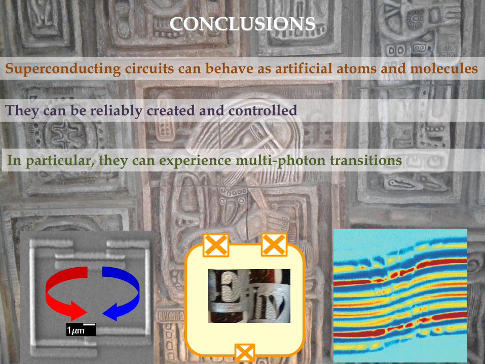
CONCLUSIONS

Superconducting circuits can behave as artificial atoms and molecules

They can be reliably created and controlled

In particular, they can experience multi-photon transitions

Φ

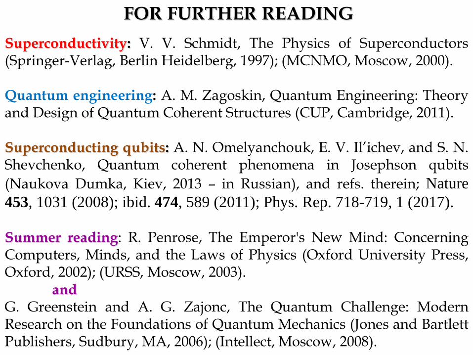
FOR FURTHER READING

Superconductivity: V. V. Schmidt, The Physics of Superconductors (Springer-Verlag, Berlin Heidelberg, 1997); (MCNMO, Moscow, 2000). Quantum engineering: A. M. Zagoskin, Quantum Engineering: Theory and Design of Quantum Coherent Structures (CUP, Cambridge, 2011). Superconducting qubits: A. N. Omelyanchouk, E. V. Il’ichev, and S. N. Shevchenko, Quantum coherent phenomena in Josephson qubits

(Naukova Dumka, Kiev, 2013 – in Russian), and refs. therein; Nature

453, 1031 (2008); ibid. 474, 589 (2011); Phys. Rep. 718-719, 1 (2017). Summer reading: R. Penrose, The Emperor's New Mind: Concerning Computers, Minds, and the Laws of Physics (Oxford University Press, Oxford, 2002); (URSS, Moscow, 2003). and G. Greenstein and A. G. Zajonc, The Quantum Challenge: Modern Research on the Foundations of Quantum Mechanics (Jones and Bartlett Publishers, Sudbury, MA, 2006); (Intellect, Moscow, 2008).