Semiclassical Treatment of High-Lying Electronic

States of H+2

T. J. Price∗,† and Chris H. Greene∗,†,‡

†Department of Physics and Astronomy, Purdue University, West Lafayette, Indiana

47907, USA

‡Purdue Quantum Center, Purdue University, West Lafayette, Indiana 47907, USA

E-mail: price198@purdue.edu; chgreene@purdue.edu

1

arX

iv:1

808.

0894

3v1

[ph

ysic

s.ch

em-p

h] 2

7 A

ug 2

018

Abstract

This work reports quantum mechanical and semiclassical WKB calculations for

energies and wave functions of high-lying 2Σ states of H+2 in atomic units. The high-

lying states presented lie in an unexplored regime, corresponding asymptotically to

H (n ≤ 145) plus a proton, with R ≤ 120, 000 a0. We compare quantum mechanical

energies, spectroscopic constants, dipole matrix elements, and phases with semiclassical

results and demonstrate a good level of agreement. The quantum mechanical phases

are determined by using Milne’s phase-amplitude procedure. Our semiclassical energies

for low-lying states are compared with those published previously in the literature.

Introduction

Many calculations for energies and wave functions of H+2 have been performed, one before

quantum mechanics was invented.1 Some have involved simplified models,2,3 while others

utilize the separability of H+2 in spheroidal coordinates to obtain accurate, almost exact

results (see e.g.4–26 and the references therein).

To our knowledge, the highest energy calculations were carried out by Pelisoli, Santos,

and Kepler24,27 for internuclear separations up to 300 a0 and dissociation limits with principal

quantum numbers n ≤ 10, to study spectral line broadening of hydrogen in the atmospheres

of white dwarf stars and laboratory plasmas; there has been discussion in the literature

regarding the lack of state-resolved data for H+2 .25,28 In this paper, we include quantum

calculations for higher excited electronic states which have not yet been calculated.

Our interest in highly excited states of H+2 was sparked by the desire to accurately

calculate long-range potential energy curves (PECs) for Rydberg molecules. A promising

approach, (generalized) local frame transformation theory,29–31 would involve such states of

H+2 . The essence of the theory is to identify systems with two regions of different approx-

imate symmetry and to interrelate the wave functions in each region. One very successful

application has been to the photoionization of non-hydrogenic Rydberg atoms in external

2

electric fields. In that application, hydrogenic states are used as a starting point. For some

long-range homonuclear Rydberg molecules, the starting point would be states of H+2 .

The states are so numerous, however, that an efficient approximation scheme is warranted.

For an approximate treatment of long-range PECs of H+2 , several approaches could be taken.

One might consider using Rayleigh-Schrodinger perturbation theory for a hydrogen atom

perturbed by a proton. Although it has been shown that accurate long-range energies of H+2

cannot be obtained with RSPT alone,32,33 semiclassical34 and other35,36 methods have been

introduced to treat the exponentially small exchange terms. Symmetry adapted perturbation

expansions have been introduced as well.37

On the other hand, semiclassical, WKB-like methods for energies and separation con-

stants of H+2 have also led to good agreement with quantum results,38–47 and we chose to

take that approach. Existing semiclassical treatments of H+2 are either carried out for the

general two-center Coulomb case, or are refined for accurate treatment of the lowest-lying

states, or both. The analyses can be complicated because of the presence of a potential

barrier between the two nuclei. Some authors go around the classical turning points in the

complex plane to derive quantization conditions that include reflection just above the bar-

rier,39–41,43 while others utilize uniform approaches to derive quantization conditions that

account for the coalescence of the classical turning points at the barrier top.38,42,44–47 While

these refinements are essential for the lowest-lying states of H+2 , for higher states, only very

small portions of the PECs involve energies near the height of the barrier, and a simple

treatment of the system can supplant more refined methods with little loss of accuracy.

We derive quantization conditions by a simple WKB treatment, with tunneling taken into

account, drawing on some results from the literature, namely a Langer-type48 modification

for H+2

39 and the connection formula for a first-order pole as applied to H+2 .40 We compare

our WKB energies with those of Strand and Reinhardt38 and Gershtein et al.,39 and confirm

that for low-lying states our approach leads to insufficient accuracy because the top of the

barrier is in an important region of the potential. For higher states, however, very good

3

accuracy is achieved with our quantization conditions; the ν values agree to three or four

decimal places except for in small regions of each potential curve near the barrier top.

In this work, we also compare quantum and semiclassical wave functions; to our knowl-

edge such a comparison has not been previously reported. Dipole matrix elements with the

ground state are presented, along with the phases of the wave functions. For the phase

comparisons, we implement the Milne phase-amplitude procedure49 as applied to H+2 ,26 with

the Milne equation expressed as a third order, linear differential equation.50,51

Since we will compare with their results, we now briefly summarize the approaches of

Strand and Reinhardt38 and Gershtein et al.39

Strand and Reinhardt38 have derived quantization conditions and wave functions us-

ing both a primitive and uniform WKB approach. In particular, Strand and Reinhardt

have emphasized the non-uniqueness of the variable transformations which lead to modified

quasimomenta. In order to obtain canonically invariant amplitudes and phases, they have

employed canonical transformations and the Keller-Maslov quantization conditions, which

assume a single classical allowed region, to determine primitive WKB solutions; as such,

these results do not incorporate tunneling through the barrier. To incorporate tunneling

effects, Strand and Reinhardt use the parabolic uniform approximation,52 where parabolic

cylinder functions are used as comparison functions rather than exponentials.

Strand and Reinhardt determine wave functions that have the same form as those given

by Gershtein et al.39 Gershtein et al. used modified, in this case referred to as Bethe-modified,

“quasimomenta” that agree with the momenta in the separated Hamilton-Jacobi (HJ) equa-

tion. Using these forms of the quasimomenta, Gershtein et al. treated the system using

the “complex method”,53–55 which was invented by Zwaan and involves going around the

classical turning points in the complex plane.

4

Theoretical Methods

Quantum Treatment

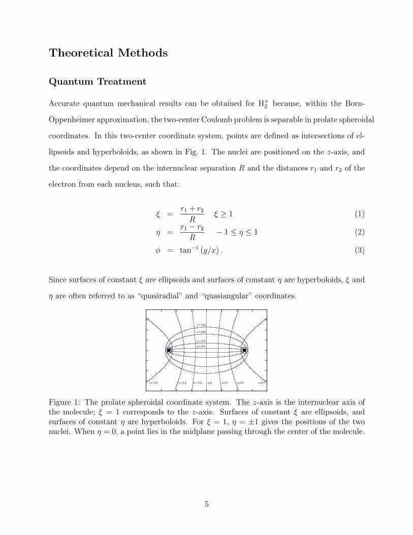
Accurate quantum mechanical results can be obtained for H+2 because, within the Born-

Oppenheimer approximation, the two-center Coulomb problem is separable in prolate spheroidal

coordinates. In this two-center coordinate system, points are defined as intersections of el-

lipsoids and hyperboloids, as shown in Fig. 1. The nuclei are positioned on the z-axis, and

the coordinates depend on the internuclear separation R and the distances r1 and r2 of the

electron from each nucleus, such that:

ξ =r1 + r2R

ξ ≥ 1 (1)

η =r1 − r2R

− 1 ≤ η ≤ 1 (2)

φ = tan−1 (y/x) . (3)

Since surfaces of constant ξ are ellipsoids and surfaces of constant η are hyperboloids, ξ and

η are often referred to as “quasiradial” and “quasiangular” coordinates.

η=0 η=0.3 η=0.6 η=0.9η=−0.3η=−0.6η=−0.9

ξ=1.001

ξ=1.010

ξ=1.050

ξ=1.100

Figure 1: The prolate spheroidal coordinate system. The z-axis is the internuclear axis ofthe molecule; ξ = 1 corresponds to the z-axis. Surfaces of constant ξ are ellipsoids, andsurfaces of constant η are hyperboloids. For ξ = 1, η = ±1 gives the positions of the twonuclei. When η = 0, a point lies in the midplane passing through the center of the molecule.

5

The stationary state wave function Ψ for H+2 can be expressed as

Ψ(ξ, η, φ) =Nελ X(ξ)√

ξ2 − 1

N(η)√1− η2

eimφ√2π, (4)

where Nελ is a normalization constant and X(ξ) and N(η) satisfy

[d2

dξ2+

{γ2 +

2Rξ−λξ2−1

+(1−m2)

(ξ2−1)2

}]X(ξ) = 0 (5)[

d2

dη2+

{γ2 +

λ

1−η2+

(1−m2)

(1−η2)2

}]N(η) = 0 (6)

In Eqs. 5 and 6, γ2 = εR2/2 depends on the electronic energy ε, and − (γ2 + λ) is a shared

separation constant. Each state is characterized by a set of node numbers {nη, nξ, nφ}, with

nη even for gerade and odd for ungerade states.

The physical significance of λ has been elucidated by Erikson and Hill56 and Coulson

and Joseph.57 As the internuclear separation R decreases to 0 and the system becomes He+,

λ → l(l + 1). As R approaches infinity, λ becomes a component of the eccentricity, or

Runge-Lenz, vector.

Erikson and Hill56 also show that the separation constant, − (γ2 + λ), is the third con-

stant of the motion; note that within the WKB approximation − (γ2 + λ−m2) is the barrier

height in the η coordinate. Owing to this extra symmetry, two potential curves that are oth-

erwise identical (e.g. two 2Σ states) may cross if they don’t have the same λ.57 One example

is the crossing of the 2sσg and 3dσg states near R = 4 a0. Avoided crossings are still pos-

sible because the electron moves in a potential that transitions from a single to a double

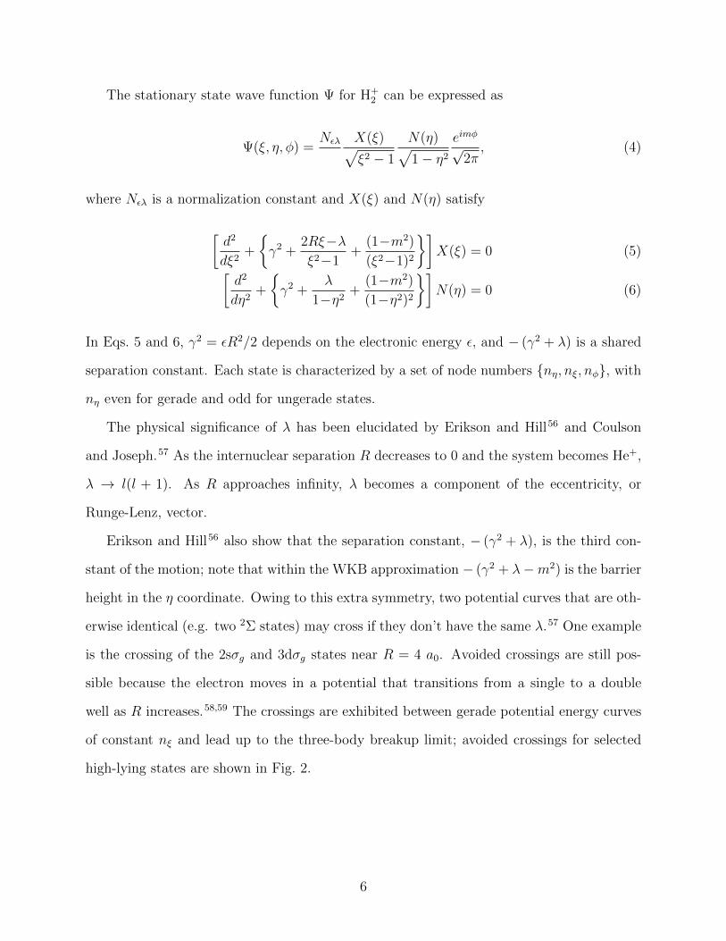
well as R increases.58,59 The crossings are exhibited between gerade potential energy curves

of constant nξ and lead up to the three-body breakup limit; avoided crossings for selected

high-lying states are shown in Fig. 2.

6

210

220

230

90000 100000

ν 2

R (a0)

Gerade states, nξ=0, nη=262−290

(a)

200

210

220

230

70000 90000 110000

ν 2

R (a0)

Gerade states, nξ=0, nη=262−290

R=70K 81K 90K 110K

nη=270

(b)

−14

−10

−6

−0.4 −0.2 0.0 0.2 0.4

Effective p

ote

ntial (1

04 E

h)

η

N(η) for (270,0): normalized to 2000 au

R=110,000 a0

R= 90,000 a0

R= 81,000 a0

R= 70,000 a0

(c)

Figure 2: Ridge of avoided crossings shown for states with nξ = 0 and nη = 262–290.

Panel (a) shows the ν2(=√−2/ε) values as a function of R; one can clearly see the avoided

crossings. Panel (b) highlights in red the curve for the state (nη, nξ) = (270, 0). Panel (c)shows wave functions for (nη, nξ) = (270, 0) for values of R corresponding to the verticallines in Panel (b). As R increases, the potential in which the electron moves transitions froma single to a double well, and the wave function markedly changes character.

7

Numerical details, Estimated Accuracy

Quantum mechanical calculations for states with nη ranging from 0 to 292 have been carried

out for states that correspond asymptotically to H (n ≤ 145) plus a proton. Our highest

energy calculations extend out to R ≤ 120, 000 a0.

In these calculations Eq. 6 is solved for the separation constants of states satisfying either

gerade or ungerade boundary conditions at η = 0. This gave a set of possible pairs (γ2, λ)

for each nη. Next, using those separation constants, Eq. 5 is solved for the energies of states

at fixed R. The shooting method accurately solves both Eqs. 5 and 6, with series expansions

for N(η) near η = −15 and for X(ξ) near ξ = 14 matched to numerically propagated wave

functions determined by a 4-point predictor corrector method. In solving Eq. 5, the large

ξ boundary condition is imposed where the wave function has decreased by 20 orders of

magnitude within a WKB approximation. The numerical integration was performed on a

square root mesh, with xη =√η + 1 and xξ =

√ξ − 1.

Accuracy was assessed by comparing calculated energies with results in the literature

for lower-lying states, and by comparing our tabulated λ values with those obtained using

Mathematica’s60 algorithm. Madsen and Peek10 report energies for the 20 lowest states of

H+2 up to R = 150 a0, and our results typically agree to the 12 decimal places reported,

except for states that are high up on the repulsive walls, where the agreement diminishes to

8 digits. Our λ values agreed with those given by Mathematica’s60 algorithm to 8–10 decimal

places, except for very large λ where that algorithm frequently converges to erroneous values

of λ.

In addition, for comparisons between phases of the quantum and semiclassical wave

functions, we have solved Eqs. 5 and 6 using the Milne phase-amplitude procedure49 with

the proper boundary conditions for H+2 .26 The Milne phase-amplitude procedure involves

solving the differential equation

[d2

dx2+ k2(x)

]ψ(x) = 0 (7)

8

exactly by calculating an amplitude α(x) such that the wave function satisfies

ψ(x) = Nα(x) sin

(∫ x

α−2(x′) dx′ + φ0

), (8)

where N is a normalization constant, and where α(x) is any particular solution of the non-

linear second-order equation

[d2

dx2+ k2(x)

]α(x) = α−3(x). (9)

The WKB approximation amounts to replacing α(x′) with 1/√|k(x′)|. Equation 9 can be

reexpressed as a third order, linear differential equation.50,51

The amplitude α(x) depends on the regular, ψ(x), and an irregular, ψ(x), solution of

Eq. 7 in the following way:

α2(x) = A (ψ(x))2 +B(ψ(x)

)2+ 2Cψ(x)ψ(x), (10)

where (AB − C2)−1/2

is equal to the Wronskian, W , between ψ(x) and ψ(x). For very small

ξ or η, the regular solutions X(ξ) and N(η) approach

X(ξ) →ξ→1

(ξ2−1

)1/2 × const. (11)

N(η) →η→−1

(1−η2

)1/2 × const. (12)

and so an irregular solution has the behavior

X(ξ) →ξ→1

(ξ2−1

)1/2ln(ξ2−1)× const. (13)

N(η) →η→−1

(1−η2

)1/2ln(1−η2)× const. . (14)

.

The wave function in Eq. 8 must satisfy the appropriate boundary conditions26 for H+2 .

9

The first boundary condition, that X(ξ) or N(η) are zero when ξ = 1 or η = −1, is satisfied

by expressing the wave functions as

X(ξ) = Nξα(ξ) sin

(∫ ξ

1

α−2(ξ′) dξ′)

(15)

N(η) = Nηα(η) sin

(∫ η

−1α−2(η′) dη′

)(16)

where η ≤ 0 in Eq. 16. The second boundary condition puts a constraint on the total phase

and yields quantization conditions in η and ξ; the total phase is the phase parameter β used

in quantum-defect theory. The phase of X(ξ) must satisfy the condition

∫ ∞1

α−2(ξ) dξ = (nξ + 1)π (17)

Above the barrier, the total phase of N(η) satisfies

2

∫ 0

−1α−2(η) dη = (nη + 1)π (18)

while below the barrier

2

∫ 0

−1α−2(η) dη = (nη + 1)π or (19)∫ 0

−1α−2(η) dη =

(nη2

+ 1)π−tan−1

(2α(0)

dα−2/dη|η=0

)(20)

depending on whether the state is ungerade (Eq. 19) or gerade (Eq. 20).

To solve for the Milne function, the third order, linear differential equation50,51 is solved

for the amplitude α from a point in the classical region23 with a 4-point predictor corrector

method; for the boundary condition at this point we used an iterative method introduced

by Seaton and Peach.61 The correct phase of the solution for small ξ or η near the singular

points is ensured by implementing the variable transformations xξ = log(ξ − 1) and xη =

log(η + 1), integrated from x0 = −350; then a formula of Korsch and Laurent62 evaluates

10

the contribution to the phase from x < −350. Korsch and Laurent’s formula62 is given by

∫α−2(x) dx = − tan−1

(WC +

WAψ(x)

ψ(x)

)+ const. (21)

where A and C are constants in Eq. 10. After substituting Eqs. 11 and 13 or Eqs. 12 and

14 into Eq. 10, one finds that the phase integral

∫α−2(ξ) dξ = const×

∫dξ

(ξ2 − 1) (ln(ξ2 − 1) + const)2or (22)∫

α−2(η) dη = const×∫

dη

(1− η2) (ln(1− η2) + const)2(23)

has the form

∫ x0

−∞

dx

ax2 + bx+ c=

(2 tan−1

(2ax0 + b√4ac− b2

)+ π

)/√

4ac− b2. (24)

where x is either xξ or xη, and where the right-hand side of Eq. 24 has the form of Eq. 21.

The constants a, b, and c are readily determined from a least-squares fit63 to exp(x)α−2(x).

Our main purpose here is to compare to semiclassical results, so the calculations pre-

sented here are based on the accurate separation constants already obtained with the shoot-

ing method. (One could also determine these constants by using the Milne quantization

conditions in η, Eqs. 18–20.)

Semiclassical WKB Treatment

The semiclassical WKB treatment of H+2 is relatively straightforward, but there are two

complications that have been discussed in the literature. The first is that the ranges of ξ and

η do not extend from −∞ to ∞; this is overcome by making a Langer-type modification to

the terms in the curly brackets of Eqs. 5 and 6, which we refer to as the “local momenta.”

The second difficulty arises for 2Σ states, because even the modified local momenta, or

“quasimomenta,” exhibit simple poles in the classically accessible regions. The present

11

section discusses the derivation of quantization conditions for 2Σ states of H+2 in light of

these complications.

As was pointed out by Strand and Reinhardt38 and by Gershtein et al.,39 Langer-type

corrections to the local momenta in Eqs. 5 and 6 are not unique. For instance, the trans-

formations x = tan (πη/2) and x = tanh−1(η) both involve a range of x that extends from

−∞ to ∞, but each leads to a different quasimomentum. To avoid this issue, Strand and

Reinhardt perform an analysis using canonical invariants.38 On the other hand, Gershtein et

al. use quasimomenta which agree with the momenta of the classical Hamilton-Jacobi (HJ)

equation:

k2L(η) =−m2

(1− η2)2+ γ2 +

λ

1− η2(25)

k2L(ξ) =−m2

(ξ2 − 1)2+ γ2 +

2Rξ − λξ2 − 1

, (26)

The quasimomenta in Eqs. 25 and 26 are sometimes referred to as “Bethe-modified,” and

we will use these forms in our analysis. (Strand and Reinhardt38 obtain wave functions in

the classical region with the same form as in Gershtein et al.39)

Different procedures for determining Langer-type modifications for general systems have

been discussed64–66 and are not our focus here, but we do wish to make a few comments

on this connection to the HJ equation. Farrelly and Reinhardt67 have shown that for hy-

drogen in a uniform electric field, the usual quasimomenta in either parabolic and squared

parabolic coordinates, in which −m2 replaces (1 − m2), also agree with the momenta in

the separated HJ equation. Moreover, the Langer modification for the hydrogen atom in

spherical coordinates gives a radial quasimomentum that agrees with the corresponding

quantity in the HJ equation, provided one identifies the classical angular momentum L with

(l+ 1/2)~.68 In general, for a separated, time independent 3D problem, using such quasimo-

menta leads to a total wave function that depends on the classical action in the following

way. Suppose the WKB wave function for each separate coordinate xk is eiSk(xk)/~, with

12

p2k(xk) = (dSk(xk)/dxk)2 in the zeroth order of ~/i. If the corrected quasimomenta pk(xk)

are the same as the momenta in the separated HJ equation, then one can identify the classi-

cal action as the sum S(x1, x2, x3, t) = S1(x1) + S2(x2) + S3(x3)− Et; the total WKB wave

function eiS(x1,x2,x3,t)/~ is expressed in terms of the classical action and is partitioned in a very

natural way, ei∑

k Sk(xk)/~. Of course in general the WKB wave function for each coordinate

is some linear combination of e±iSk(xk)/~, and there can be additional cross terms that appear

in the total wave function.

We now consider the quasimomenta in Eqs. 25 and 26. For 2Σ states, there are two roots

ηc of Eq. 25:

ηc = ±

√γ2 + λ

γ2. (27)

When γ2 +λ is negative, the ηc correspond to two real roots. Since λ ≥ 0 for H+2 , these roots

are always between η = ±1. As γ2 + λ approaches zero, the two roots coalesce to ηc = 0,

and the ηc are no longer simple zeros of Eq. 25. When γ2 + λ is positive, the roots ηc are

purely imaginary complex conjugates. In other words, there is a potential barrier in the η

coordinate with the separation constant, −(γ2 + λ), as its height; the separation constant is

the third constant of the motion for the system. The barrier in the η coordinate depends

on R, ε, and the number of nodes in N(η). An example in which the electron is below the

barrier is shown in Panel (a) of Fig. 3. Note that the poles at η = ±1 are in the classically

accessible regions.

In contrast, the quasimomentum in ξ, defined by Eq. 26, does not exhibit a potential

barrier. Instead, it has either one or no minimum. If λ ≤ 2R, then there is no minimum in

k2L(ξ), and the pole at ξ = 1 is in the classical region. If λ > 2R, there is a single minimum

which bars the electron from the region near the internuclear axis. This minimum moves

further out in ξ as λ increases past 2R. For the case where R = 0, that is, for He+, λ is

l(l + 1) and this minimum in ξ is associated with the combined centrifugal and Coulomb

potentials. In the general case of nonzero R, for a fixed energy, λ increases with nη; with

sufficient “angular” excitation, a minimum appears in k2L(ξ).

13

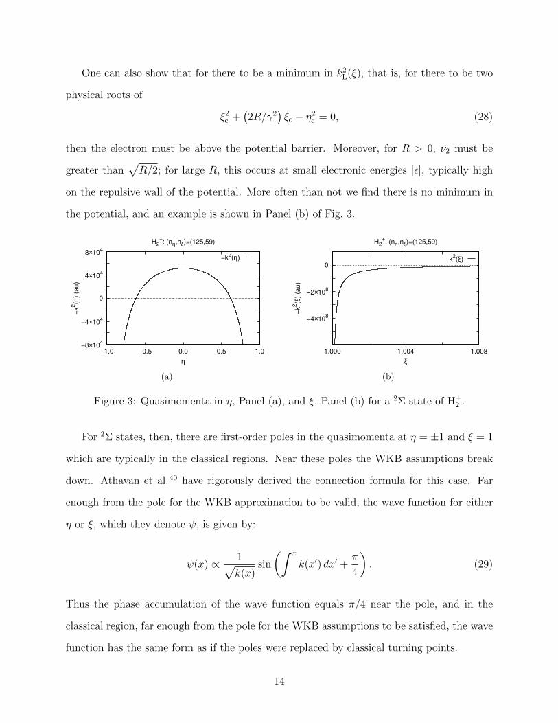
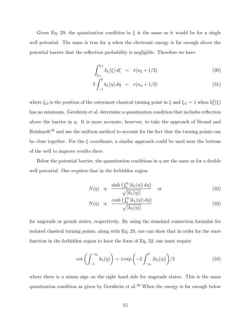
One can also show that for there to be a minimum in k2L(ξ), that is, for there to be two

physical roots of

ξ2c +(2R/γ2

)ξc − η2c = 0, (28)

then the electron must be above the potential barrier. Moreover, for R > 0, ν2 must be

greater than√R/2; for large R, this occurs at small electronic energies |ε|, typically high

on the repulsive wall of the potential. More often than not we find there is no minimum in

the potential, and an example is shown in Panel (b) of Fig. 3.

−8×104

−4×104

0

4×104

8×104

−1.0 −0.5 0.0 0.5 1.0

−k

2(η

) (a

u)

η

H2+: (nη,nξ)=(125,59)

−k2(η)

(a)

−4×108

−2×108

0

1.000 1.004 1.008

−k

2(ξ

) (a

u)

ξ

H2+: (nη,nξ)=(125,59)

−k2(ξ)

(b)

Figure 3: Quasimomenta in η, Panel (a), and ξ, Panel (b) for a 2Σ state of H+2 .

For 2Σ states, then, there are first-order poles in the quasimomenta at η = ±1 and ξ = 1

which are typically in the classical regions. Near these poles the WKB assumptions break

down. Athavan et al.40 have rigorously derived the connection formula for this case. Far

enough from the pole for the WKB approximation to be valid, the wave function for either

η or ξ, which they denote ψ, is given by:

ψ(x) ∝ 1√k(x)

sin

(∫ x

k(x′) dx′ +π

4

). (29)

Thus the phase accumulation of the wave function equals π/4 near the pole, and in the

classical region, far enough from the pole for the WKB assumptions to be satisfied, the wave

function has the same form as if the poles were replaced by classical turning points.

14

Given Eq. 29, the quantization condition in ξ is the same as it would be for a single

well potential. The same is true for η when the electronic energy is far enough above the

potential barrier that the reflection probability is negligible. Therefore we have

∫ ξc2

ξc1

kL(ξ) dξ = π(nξ + 1/2) (30)

2

∫ 0

−1kL(η) dη = π(nη + 1/2) (31)

where ξc2 is the position of the outermost classical turning point in ξ and ξc1 = 1 when k2L(ξ)

has no minimum. Gershtein et al. determine a quantization condition that includes reflection

above the barrier in η. It is more accurate, however, to take the approach of Strand and

Reinhardt38 and use the uniform method to account for the fact that the turning points can

be close together. For the ξ coordinate, a similar approach could be used near the bottom

of the well to improve results there.

Below the potential barrier, the quantization conditions in η are the same as for a double

well potential. One requires that in the forbidden region

N(η) ∝sinh

(∫ η0|kL(η)| dη

)√|kL(η)|

or (32)

N(η) ∝cosh

(∫ η0|kL(η)| dη

)√|kL(η)|

(33)

for ungerade or gerade states, respectively. By using the standard connection formulae for

isolated classical turning points, along with Eq. 29, one can show that in order for the wave

function in the forbidden region to have the form of Eq. 32, one must require

cot

(∫ −ηc−1

kL(η)

)= ±exp

(−2

∫ 0

−ηc|kL(η)|

)/2 (34)

where there is a minus sign on the right hand side for ungerade states. This is the same

quantization condition as given by Gershtein et al.39 When the energy is far enough below

15

the barrier, the right-hand side of Eq. 34 is negligible, and the quantization conditions reduce

to

2

∫ ηc

−1kL(η) dη = π(nη + 1) or (35)

= πnη (36)

depending on whether the state has gerade (Eq. 35) or ungerade (Eq. 36) symmetry.

In the classical region, the WKB wave functions have the form

X(ξ) ∝

√1

kL(ξ)sin

(∫ ξc2

ξc1

kL(ξ) + π/4

)(37)

N(η) ∝

√1

kL(η)sin

(∫ −ηc−1

kL(η) + π/4

), (38)

where the η wave function is either symmetric or antisymmetric about η = 0. These forms

agree with those given by Strand and Reinhardt38 and Gershtein et al.39

Near the classical turning points, when they are not too close together, the quasimomen-

tum k2L can be defined to be 2α(x− xc) and, with z := −(2α)1/3(x− xc), one has

X(ξ) ∝√π

(2α)1/6sin

(∫ ξc2

ξc1

kL(ξ)

)Ai(z) (39)

N(η) ∝√π

(2α)1/6

{sin

(∫ −ηc−1

kL(η)

)Ai(z)

+ cos

(∫ −ηc−1

kL(η)

)Bi(z)

}(40)

where Ai(z) and Bi(z) are the Airy functions of the first and second kind, and where Eq. 40

applies to states below the potential barrier.

Finally, in the forbidden region

X(ξ) ∝ 1√|kL(ξ)|

exp

(−∫ ∞ξc2

|kL(ξ)| dξ)

(41)

16

and N(η) has the form of Eq. 32 for ungerade or of Eq. 33 for gerade states.

Results and Discussion

Energies

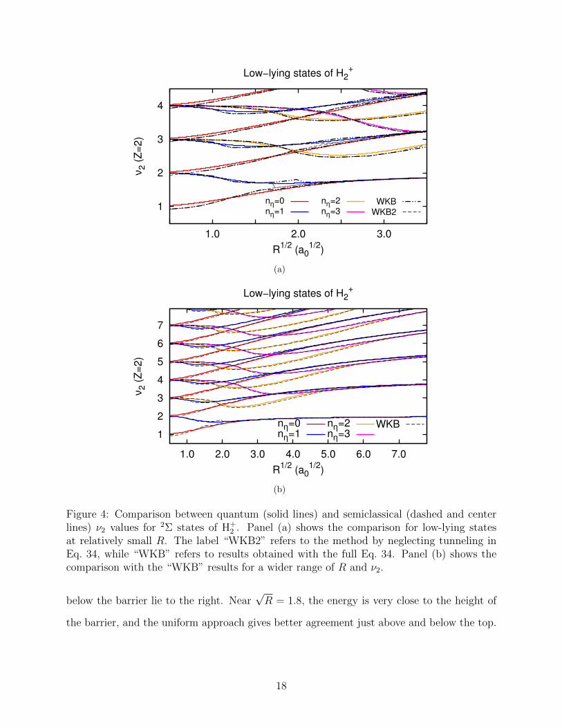
Figure 4 shows a comparison between our semiclassical and quantum mechanical values of

ν2(=√−2/ε) for low-lying states of H+

2 . Panel (a), which shows the comparison for a

smaller range than Panel (b), illustrates where the tunneling rate is large enough that the

right-hand side of Eq. 34 is non-negligible; results obtained by using the full Eq. 34 are

labeled “WKB,” while results obtained by using Eqs. 35 or 36 are labeled “WKB2.” Of

course, it’s only important to account for the true tunneling rate by using Eq. 34 near the

barrier tops, where the gerade-ungerade splitting is just starting to manifest itself in the

figure. There are bumps, however, in the “WKB” energies very close to the barrier tops

where the turning points cannot be considered isolated. In Panel (a) of Fig. 4 one can see,

for instance, a bump near R = 3.5 a0 for the state (nη, nξ) = (1, 0) where the ν2 value is

overestimated. Accounting for reflections just above the barrier, as was done by Gershtein

et al.,39 diminishes but does not remove the bumps near the barrier tops, which can be seen

in their Fig. 4.

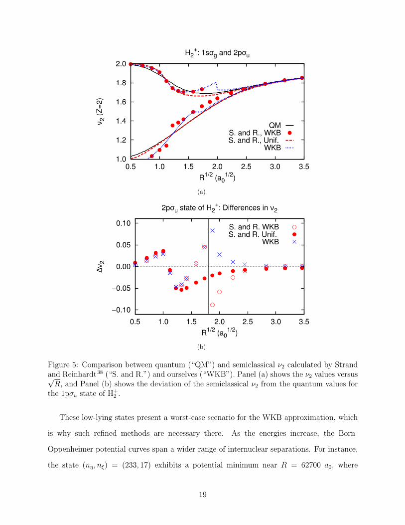
Strand and Reinhardt38 account for the proximity of the turning points near the height

of the barrier with a uniform approach. Panel (a) of Fig. 5 compares the ν2 values they

obtained by using the uniform approach (dashed lines) with our WKB results (dotted lines),

WKB results38 that neglect tunneling in Eq. 34 (solid circles), and the quantum values (solid

lines). Accurately determining the tunneling integral in Eq. 34 improves results below the

barrier top. Then the energies can be further refined by using a uniform approach, which

gives better results where the turning points are close together. Panel (b) of Fig. 5 shows

the difference between the quantum mechanical and semiclassical values of ν2 for the 1pσu

state. Energies above the potential barrier lie to the left of the vertical line, while energies

17

1

2

3

4

1.0 2.0 3.0

ν 2 (

Z=

2)

R1/2

(a01/2

)

Low−lying states of H2+

nη=0

nη=1

nη=2

nη=3WKB

WKB2

(a)

1

2

3

4

5

6

7

1.0 2.0 3.0 4.0 5.0 6.0 7.0

ν 2 (

Z=

2)

R1/2

(a01/2

)

Low−lying states of H2+

nη=0nη=1

nη=2nη=3

WKB

(b)

Figure 4: Comparison between quantum (solid lines) and semiclassical (dashed and centerlines) ν2 values for 2Σ states of H+

2 . Panel (a) shows the comparison for low-lying statesat relatively small R. The label “WKB2” refers to the method by neglecting tunneling inEq. 34, while “WKB” refers to results obtained with the full Eq. 34. Panel (b) shows thecomparison with the “WKB” results for a wider range of R and ν2.

below the barrier lie to the right. Near√R = 1.8, the energy is very close to the height of

the barrier, and the uniform approach gives better agreement just above and below the top.

18

1.0

1.2

1.4

1.6

1.8

2.0

0.5 1.0 1.5 2.0 2.5 3.0 3.5

ν 2 (

Z=

2)

R1/2

(a01/2

)

H2+: 1sσg and 2pσu

QMS. and R., WKBS. and R., Unif.

WKB

(a)

−0.10

−0.05

0.00

0.05

0.10

0.5 1.0 1.5 2.0 2.5 3.0 3.5

∆ν2

R1/2

(a01/2

)

2pσu state of H2+: Differences in ν2

S. and R. WKBS. and R. Unif.

WKB

(b)

Figure 5: Comparison between quantum (“QM”) and semiclassical ν2 calculated by Strandand Reinhardt38 (“S. and R.”) and ourselves (“WKB”). Panel (a) shows the ν2 values versus√R, and Panel (b) shows the deviation of the semiclassical ν2 from the quantum values for

the 1pσu state of H+2 .

These low-lying states present a worst-case scenario for the WKB approximation, which

is why such refined methods are necessary there. As the energies increase, the Born-

Oppenheimer potential curves span a wider range of internuclear separations. For instance,

the state (nη, nξ) = (233, 17) exhibits a potential minimum near R = 62700 a0, where

19

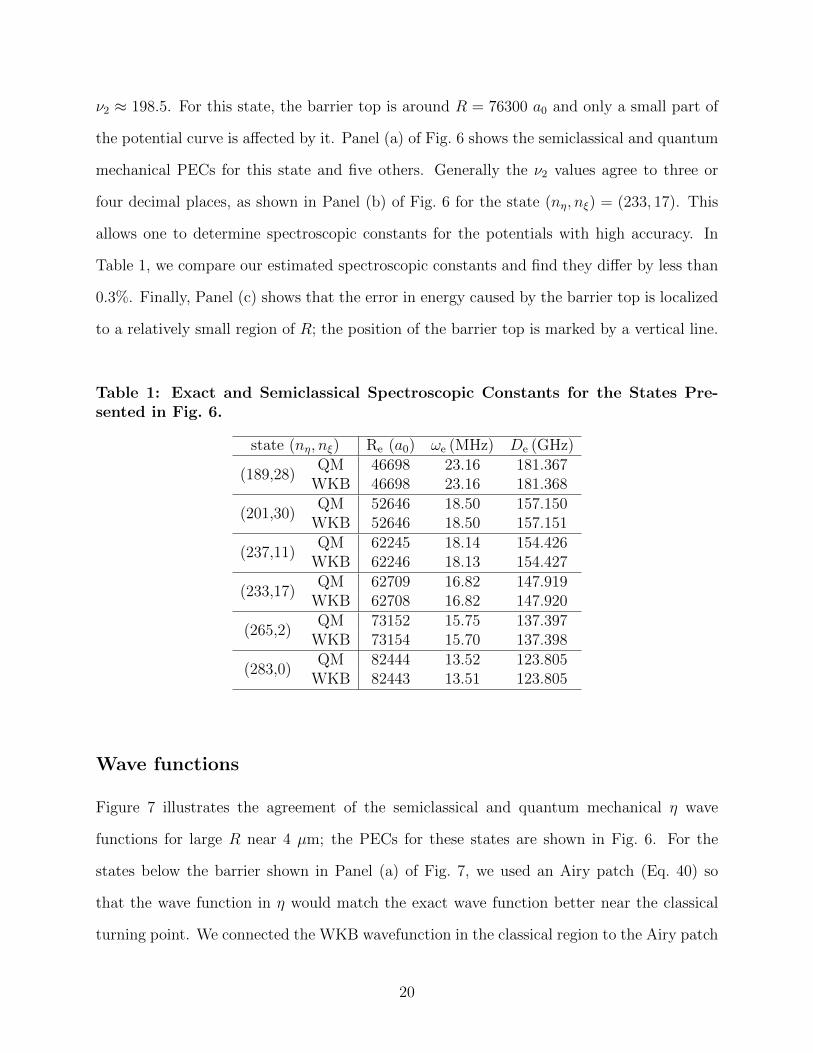
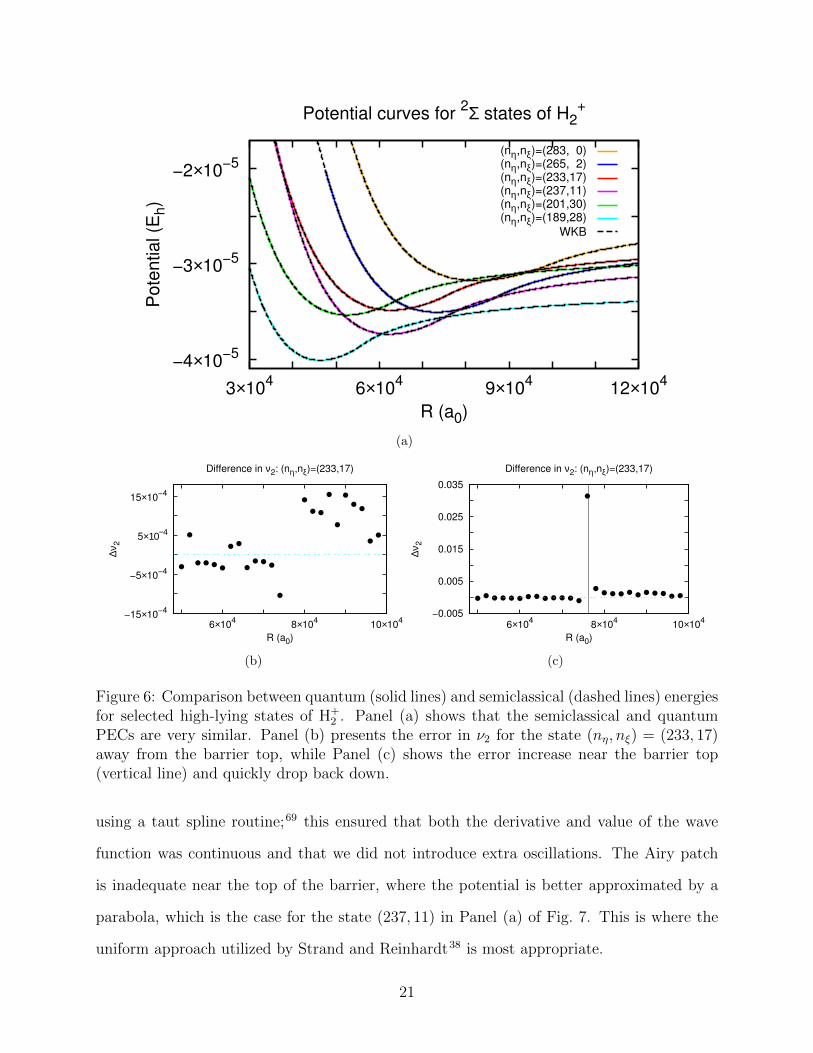
ν2 ≈ 198.5. For this state, the barrier top is around R = 76300 a0 and only a small part of

the potential curve is affected by it. Panel (a) of Fig. 6 shows the semiclassical and quantum

mechanical PECs for this state and five others. Generally the ν2 values agree to three or

four decimal places, as shown in Panel (b) of Fig. 6 for the state (nη, nξ) = (233, 17). This

allows one to determine spectroscopic constants for the potentials with high accuracy. In

Table 1, we compare our estimated spectroscopic constants and find they differ by less than

0.3%. Finally, Panel (c) shows that the error in energy caused by the barrier top is localized

to a relatively small region of R; the position of the barrier top is marked by a vertical line.

Table 1: Exact and Semiclassical Spectroscopic Constants for the States Pre-sented in Fig. 6.

state (nη, nξ) Re (a0) ωe (MHz) De (GHz)

(189,28)QM 46698 23.16 181.367

WKB 46698 23.16 181.368

(201,30)QM 52646 18.50 157.150

WKB 52646 18.50 157.151

(237,11)QM 62245 18.14 154.426

WKB 62246 18.13 154.427

(233,17)QM 62709 16.82 147.919

WKB 62708 16.82 147.920

(265,2)QM 73152 15.75 137.397

WKB 73154 15.70 137.398

(283,0)QM 82444 13.52 123.805

WKB 82443 13.51 123.805

Wave functions

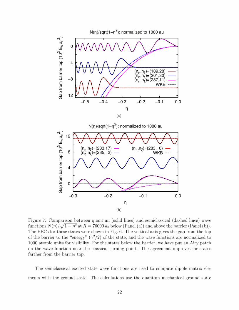
Figure 7 illustrates the agreement of the semiclassical and quantum mechanical η wave

functions for large R near 4 µm; the PECs for these states are shown in Fig. 6. For the

states below the barrier shown in Panel (a) of Fig. 7, we used an Airy patch (Eq. 40) so

that the wave function in η would match the exact wave function better near the classical

turning point. We connected the WKB wavefunction in the classical region to the Airy patch

20

−4×10−5

−3×10−5

−2×10−5

3×104

6×104

9×104

12×104

Pote

ntial (E

h)

R (a0)

Potential curves for 2Σ states of H2

+

(nη,nξ)=(283, 0)(nη,nξ)=(265, 2)(nη,nξ)=(233,17)(nη,nξ)=(237,11)(nη,nξ)=(201,30)(nη,nξ)=(189,28)

WKB

(a)

−15×10−4

−5×10−4

5×10−4

15×10−4

6×104

8×104

10×104

∆ν2

R (a0)

Difference in ν2: (nη,nξ)=(233,17)

(b)

−0.005

0.005

0.015

0.025

0.035

6×104

8×104

10×104

∆ν2

R (a0)

Difference in ν2: (nη,nξ)=(233,17)

(c)

Figure 6: Comparison between quantum (solid lines) and semiclassical (dashed lines) energiesfor selected high-lying states of H+

2 . Panel (a) shows that the semiclassical and quantumPECs are very similar. Panel (b) presents the error in ν2 for the state (nη, nξ) = (233, 17)away from the barrier top, while Panel (c) shows the error increase near the barrier top(vertical line) and quickly drop back down.

using a taut spline routine;69 this ensured that both the derivative and value of the wave

function was continuous and that we did not introduce extra oscillations. The Airy patch

is inadequate near the top of the barrier, where the potential is better approximated by a

parabola, which is the case for the state (237, 11) in Panel (a) of Fig. 7. This is where the

uniform approach utilized by Strand and Reinhardt38 is most appropriate.

21

−12

−8

−4

0

−0.5 −0.4 −0.3 −0.2 −0.1 0.0

Gap fro

m b

arr

ier

top (

10

3 E

h a

02)

η

N(η)/sqrt(1−η2): normalized to 1000 au

(nη,nξ)=(189,28)(nη,nξ)=(201,30)(nη,nξ)=(237,11)

WKB

(a)

0

4

8

12

−0.3 −0.2 −0.1 0.0

Gap fro

m b

arr

ier

top (

10

3 E

h a

02)

η

N(η)/sqrt(1−η2): normalized to 1000 au

(nη,nξ)=(233,17)(nη,nξ)=(265, 2)

(nη,nξ)=(283, 0)WKB

(b)

Figure 7: Comparison between quantum (solid lines) and semiclassical (dashed lines) wavefunctionsN(η)/

√1− η2 atR = 76000 a0 below (Panel (a)) and above the barrier (Panel (b)).

The PECs for these states were shown in Fig. 6. The vertical axis gives the gap from the topof the barrier to the “energy” (γ2/2) of the state, and the wave functions are normalized to1000 atomic units for visibility. For the states below the barrier, we have put an Airy patchon the wave function near the classical turning point. The agreement improves for statesfarther from the barrier top.

The semiclassical excited state wave functions are used to compute dipole matrix ele-

ments with the ground state. The calculations use the quantum mechanical ground state

22

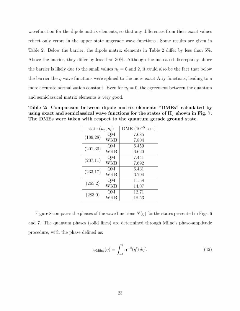
wavefunction for the dipole matrix elements, so that any differences from their exact values

reflect only errors in the upper state ungerade wave functions. Some results are given in

Table 2. Below the barrier, the dipole matrix elements in Table 2 differ by less than 5%.

Above the barrier, they differ by less than 30%. Although the increased discrepancy above

the barrier is likely due to the small values nξ = 0 and 2, it could also be the fact that below

the barrier the η wave functions were splined to the more exact Airy functions, leading to a

more accurate normalization constant. Even for nξ = 0, the agreement between the quantum

and semiclassical matrix elements is very good.

Table 2: Comparison between dipole matrix elements “DMEs” calculated byusing exact and semiclassical wave functions for the states of H+

2 shown in Fig. 7.The DMEs were taken with respect to the quantum gerade ground state.

state (nη, nξ) DME (10−5 a.u.)

(189,28)QM 7.685

WKB 7.804

(201,30)QM 6.459

WKB 6.620

(237,11)QM 7.441

WKB 7.692

(233,17)QM 6.431

WKB 6.794

(265,2)QM 11.58

WKB 14.07

(283,0)QM 12.71

WKB 18.53

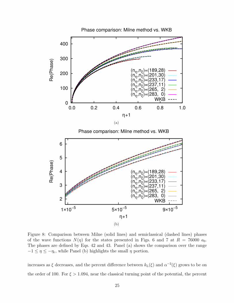
Figure 8 compares the phases of the wave functionsN(η) for the states presented in Figs. 6

and 7. The quantum phases (solid lines) are determined through Milne’s phase-amplitude

procedure, with the phase defined as:

φMilne(η) =

∫ η

−1α−2(η′) dη′. (42)

23

The dashed lines show the semiclassical phases in the classical region,

φWKB(η) =

∫ η

−1kL(η′) dη′ + π/4, η < −ηc (43)

where ηc = 0 for states above the barrier. The quantum (Eq. 42) and semiclassical (Eq. 43)

phases are most different for low values of η where the quasimomentum varies rapidly and the

WKB approximation is less accurate. This small η region is highlighted in Panel (b). The

discrepancies are still small, and over the whole range of η the quantum and semiclassical

results differ by less than 0.1%.

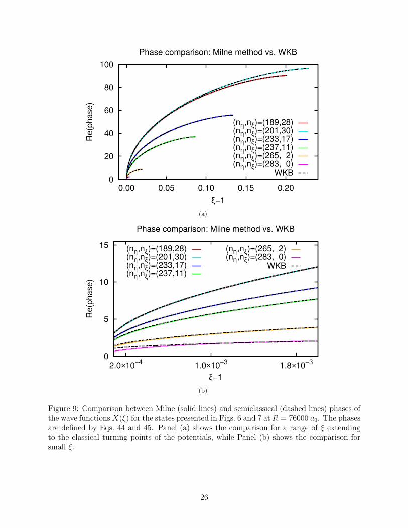
Figure 9 compares the phases of the wave functions X(ξ), defined as

φMilne(ξ) =

∫ ξ

1

α−2(ξ′) dξ′. (44)

φWKB(ξ) =

∫ ξ

ξc1

kL(ξ′) dξ′ + π/4 ξ < ξc2. (45)

Panel (b) shows that, as with the phases of N(η), the quantum (solid lines) and WKB

(dashed lines) values differ most when ξ is small. The deviation is larger for wave functions

with a smaller node number.

Figure 10 presents a typical comparison between the WKB wave number kL(ξ) and the

Milne α−2(ξ). The dotted line shows the percent difference between the two, which increases

as the WKB approximation breaks down. Approximately, the WKB assumptions are satisfied

where ∣∣∣∣ ddξ 1

kL(ξ)

∣∣∣∣ << 1 (46)

The region for which the left hand side of Eq. 46 is less than 0.1 is bracketed by the two

vertical lines in Fig. 10, with the vertical line on the left at approximately ξ = 1.003 and

the vertical line on the right at approximately ξ = 1.094. The percent difference between

kL(ξ) and α−2(ξ) is less than 0.5 within this region. For small ξ < 1.0030, kL(ξ) varies more

and more rapidly before becoming singular at ξ = 1, so that the left-hand side of Eq. 46

24

0

100

200

300

400

0.0 0.2 0.4 0.6 0.8 1.0

Re

(Ph

ase

)

η+1

Phase comparison: Milne method vs. WKB

(nη,nξ)=(189,28)(nη,nξ)=(201,30)(nη,nξ)=(233,17)(nη,nξ)=(237,11)(nη,nξ)=(265, 2)(nη,nξ)=(283, 0)

WKB

(a)

2

3

4

5

6

1×10−5

5×10−5

9×10−5

Re

(Ph

ase

)

η+1

Phase comparison: Milne method vs. WKB

(nη,nξ)=(189,28)(nη,nξ)=(201,30)(nη,nξ)=(233,17)(nη,nξ)=(237,11)(nη,nξ)=(265, 2)(nη,nξ)=(283, 0)

WKB

(b)

Figure 8: Comparison between Milne (solid lines) and semiclassical (dashed lines) phasesof the wave functions N(η) for the states presented in Figs. 6 and 7 at R = 76000 a0.The phases are defined by Eqs. 42 and 43. Panel (a) shows the comparison over the range−1 ≤ η ≤ −ηc, while Panel (b) highlights the small η portion.

increases as ξ decreases, and the percent difference between kL(ξ) and α−2(ξ) grows to be on

the order of 100. For ξ > 1.094, near the classical turning point of the potential, the percent

25

0

20

40

60

80

100

0.00 0.05 0.10 0.15 0.20

Re

(ph

ase

)

ξ−1

Phase comparison: Milne method vs. WKB

(nη,nξ)=(189,28)(nη,nξ)=(201,30)(nη,nξ)=(233,17)(nη,nξ)=(237,11)(nη,nξ)=(265, 2)(nη,nξ)=(283, 0)

WKB

(a)

0

5

10

15

2.0×10−4

1.0×10−3

1.8×10−3

Re

(ph

ase

)

ξ−1

Phase comparison: Milne method vs. WKB

(nη,nξ)=(189,28)(nη,nξ)=(201,30)(nη,nξ)=(233,17)(nη,nξ)=(237,11)

(nη,nξ)=(265, 2)(nη,nξ)=(283, 0)

WKB

(b)

Figure 9: Comparison between Milne (solid lines) and semiclassical (dashed lines) phases ofthe wave functions X(ξ) for the states presented in Figs. 6 and 7 at R = 76000 a0. The phasesare defined by Eqs. 44 and 45. Panel (a) shows the comparison for a range of ξ extendingto the classical turning points of the potentials, while Panel (b) shows the comparison forsmall ξ.

26

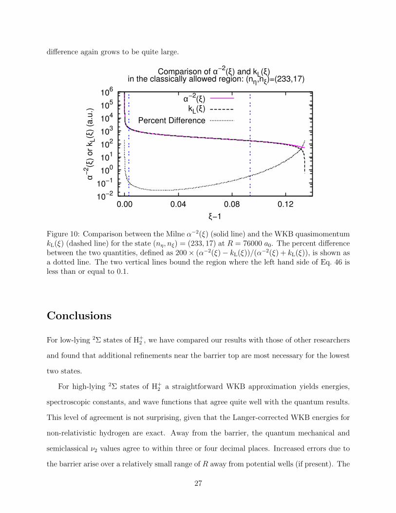
difference again grows to be quite large.

10−2

10−1

100

101

102

103

104

105

106

0.00 0.04 0.08 0.12

α−2(ξ

) o

r k

L(ξ

) (a

.u.)

ξ−1

Comparison of α−2(ξ) and kL(ξ)

in the classically allowed region: (nη,nξ)=(233,17)

Wed Aug 01, 2018 14:11:20 comparealph5.eps Windows 7

α−2(ξ)

kL(ξ)

Percent Difference

Figure 10: Comparison between the Milne α−2(ξ) (solid line) and the WKB quasimomentumkL(ξ) (dashed line) for the state (nη, nξ) = (233, 17) at R = 76000 a0. The percent differencebetween the two quantities, defined as 200× (α−2(ξ)− kL(ξ))/(α−2(ξ) + kL(ξ)), is shown asa dotted line. The two vertical lines bound the region where the left hand side of Eq. 46 isless than or equal to 0.1.

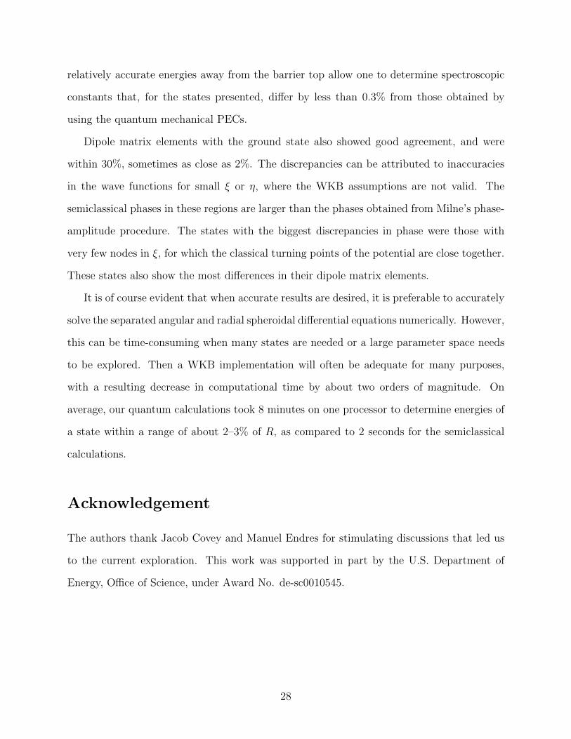
Conclusions

For low-lying 2Σ states of H+2 , we have compared our results with those of other researchers

and found that additional refinements near the barrier top are most necessary for the lowest

two states.

For high-lying 2Σ states of H+2 a straightforward WKB approximation yields energies,

spectroscopic constants, and wave functions that agree quite well with the quantum results.

This level of agreement is not surprising, given that the Langer-corrected WKB energies for

non-relativistic hydrogen are exact. Away from the barrier, the quantum mechanical and

semiclassical ν2 values agree to within three or four decimal places. Increased errors due to

the barrier arise over a relatively small range of R away from potential wells (if present). The

27

relatively accurate energies away from the barrier top allow one to determine spectroscopic

constants that, for the states presented, differ by less than 0.3% from those obtained by

using the quantum mechanical PECs.

Dipole matrix elements with the ground state also showed good agreement, and were

within 30%, sometimes as close as 2%. The discrepancies can be attributed to inaccuracies

in the wave functions for small ξ or η, where the WKB assumptions are not valid. The

semiclassical phases in these regions are larger than the phases obtained from Milne’s phase-

amplitude procedure. The states with the biggest discrepancies in phase were those with

very few nodes in ξ, for which the classical turning points of the potential are close together.

These states also show the most differences in their dipole matrix elements.

It is of course evident that when accurate results are desired, it is preferable to accurately

solve the separated angular and radial spheroidal differential equations numerically. However,

this can be time-consuming when many states are needed or a large parameter space needs

to be explored. Then a WKB implementation will often be adequate for many purposes,

with a resulting decrease in computational time by about two orders of magnitude. On

average, our quantum calculations took 8 minutes on one processor to determine energies of

a state within a range of about 2–3% of R, as compared to 2 seconds for the semiclassical

calculations.

Acknowledgement

The authors thank Jacob Covey and Manuel Endres for stimulating discussions that led us

to the current exploration. This work was supported in part by the U.S. Department of

Energy, Office of Science, under Award No. de-sc0010545.

28

References

(1) Pauli, W., Jr. Ann. Phys. (Leipzig) 1922, 68, 177.

(2) Frost, A. A. Delta-function model. I. Electronic energies of hydrogen-like atoms and

diatomic molecules. J. Chem. Phys. 1956, 25, 1150–1154.

(3) Frost, A. A.; Musulin, B. Semiempirical potential energy functions. I. The H2 and H+2

diatomic molecules. J. Chem. Phys. 1954, 22, 1017–1020.

(4) Jaffe, G. Z. Phys. 1934, 87, 535.

(5) Baber, W. G.; Hasse, H. R. Proc. Cambridge Philos. Soc. 1935, 25, 564.

(6) Bates, D. R.; Ledsham, K.; Stewart, A. L. Wave functions of the hydrogen molecular

ion. Philos. Trans. Royal Soc. A 1953, 246, 215–240.

(7) Hodge, D. B. Eigenvalues and eigenfunctions of the spheroidal wave equation. J. Math.

Phys. 1970, 11, 2308–2312.

(8) Montgomery, H. E., Jr. One-electron wavefunctions. Accurate expectation values.

Chem. Phys. Lett. 1977, 50, 455–458.

(9) Bailey, P. B. Automatic calculation of the energy levels of one-electron diatomic

molecules. J. Chem. Phys. 1978, 69, 1676–1679.

(10) Madsen, M. M.; Peek, J. M. Eigenparameters for the lowest twenty electronic states of

the hydrogen molecule ion. At. Data 1971, 2, 171–204.

(11) Boyack, R.; Lekner, J. Confluent Heun functions and separation of variables in

spheroidal coordinates. J. Math. Phys. 2011, 52, 073517 (8 pages).

(12) Scott, T. C.; Aubert-Frecon, M.; Grotendorst, J. New approach for the electronic en-

ergies of the hydrogen molecular ion. Chem. Phys. 2006, 324, 323–338.

29

(13) Leaver, E. W. Solutions to a generalized spheroidal wave equation: Teukolsky’s equa-

tions in general relativity, and the two-center problem in molecular quantum mechanics.

J. Math. Phys 1986, 27, 1238–1265.

(14) Liu, J. W. Analytical solutions to the generalized spheroidal wave equation and the

Green’s function of one-electron diatomic molecules. J. Math. Phys 1992, 33, 4026–

4036.

(15) Figueiredo, B. D. B.; Novello, M. Solutions to a spheroidal wave equation. J. Math.

Phys. 1993, 34, 3121–3132.

(16) Figueiredo, B. D. B. Generalized spheroidal wave equation and limiting cases. J. Math.

Phys. 2007, 48, 013503 (43 pages).

(17) Ponomarev, L. I.; Puzynina, T. P.; Truskova, N. F. Effective potentials of the three-

body problem in the adiabatic representation. J. Phys. B: Atom. Molec. Phys. 1978,

11, 3861–3874.

(18) Ramaker, D. E.; Peek, J. M. 2H+2 dipole strengths by asymptotic techniques. J. Phys.

B. At. Mol. Opt. Phys. 1972, 5, 2175–2181.

(19) Ramaker, D. E.; Peek, J. M. Dipole strengths involving the lowest twenty electronic

states of H+2 . Atomic Data and Nuclear Data Tables 1973, 5, 164–184.

(20) Kereselidze, T.; Chkadua, G.; Defrance, P. Coulomb Sturmians in spheroidal coordi-

nates and their application for diatomic molecular calculations. Mol. Phys. 2015, 113,

3471–3479.

(21) Kereselidze, T.; Chkadua, G.; Defrance, P.; Ogilvie, J. F. Derivation, properties and

application of Coulomb Sturmians defined in spheroidal coordinates. Mol. Phys. 2015,

114, 148–161.

30

(22) Ponomarev, L. I.; Somov, L. N. The wave functions of continuum for the two-center

problem in quantum mechanics. J. Comput. Phys. 1976, 20, 183–195.

(23) Yoo, B.; Greene, C. H. Implementation of the quantum-defect theory for arbitrary

long-range potentials. Phys. Rev. A 1986, 34, 1635–1643.

(24) Santos, M. G.; Kepler, S. O. Theoretical study of line profiles of the hydrogen perturbed

by collisions with protons. Mon. Not. R. Astron. Soc. 2012, 423, 68–79.

(25) Zammit, M. C.; Savage, J. S.; Colgan, J.; Fursa, D. V.; Kilcrease, D. P.; Bray, I.;

Fontes, C. J.; Hakel, P.; Timmermans, E. State-resolved photodissociation and radiative

association data for the molecular hydrogen ion. Astrophys. J. 2017, 851, 64 (16 pages).

(26) Froman, P. O.; Larsson, K. Phase-amplitude method for numerically exact solution of

the differential equations of the two-center Coulomb problem. J. Math. Phys. 2002, 43,

2169–2179.

(27) Pelisoli, I.; Santos, M. G.; Kepler, S. O. Unified line profiles for hydrogen perturbed by

collisions with protons: satellites and asymmetries. Mon. Not. R. Astron. Soc. 2015,

448, 2332–2343.

(28) Babb, J. F. State-resolved data for radiative association of H and H+ and for photodis-

sociation of H+2 . Astrophys. J. Supp. Series 2015, 216, 21 (3 pages).

(29) Giannakeas, P.; Greene, C. H.; Robicheaux, F. Generalized local frame transformation

theory for excited species in external fields. Phys. Rev. A 2016, 94, 013419 (9 pages).

(30) Fano, U. Stark effect of nonhydrogenic Rydberg spectra. Phys. Rev. A 1981, 24, 619–

622.

(31) Harmin, D. A. Theory of the Stark effect. Phys. Rev. A 1982, 26, 2656–2680.

31

(32) Dalgarno, A.; Lewis, J. T. The representation of long range forces by series expansions

I: The divergence of the series II: The complete perturbation calculation of long range

forces. Proc. Phys. Soc. A. 1956, 69, 57–64.

(33) Robinson, P. D. H+2 : a problem in perturbation theory. Proc. Phys. Soc. 1961, 78,

537–548.

(34) Cızek, J.; Damburg, R. J.; Graffi, S.; Grecchi, V.; Harrell, E. M., II.; Harris, J. G.;

Nakai, S.; Paldus, J.; Propin, R. K.; Silverstone, H. J. 1/R expansion for H+2 : Calcula-

tion of exponentially small terms and asymptotics. Phys. Rev. A 1986, 33, 12–33.

(35) Tang, K. T.; Toennies, J. P.; Yiu, C. L. The exchange energy of H+2 calculated from

polarization perturbation theory. J. Chem. Phys. 1991, 94, 175–183.

(36) Scott, T. C.; Babb, J. F.; Dalgarno, A.; Morgan, J. D., III Resolution of a paradox in

the calculation of exchange forces for H+2 . Chem. Phys. Lett. 1992, 203, 7266–7277.

(37) Cha lasinaski, G.; Szalewicz, K. Degenerate symmetry-adapted perturbation theory.

Convergence properties of perturbation expansions for excited states of H+2 ion. Int J

Quantum Chem. 18, 1071–1089.

(38) Strand, M. P.; Reinhardt, W. P. Semiclassical quantization of the low lying electronic

states of H+2 . J. Chem. Phys. 1979, 70, 3812–3827.

(39) Gershtein, S. S.; Ponomarev, L. I.; Puzynina, T. P. A quasiclassical approximation in

the two-center problem. J. Exptl. Theoret. Phys. (U.S.S.R) 1965, 48, 632–643.

(40) Athavan, N.; Froman, P. O.; Froman, N.; Lakshmanan, M. Quantal two-center Coulomb

problem treated by means of the phase-integral method. I. General theory. J. Math.

Phys. 2001, 42, 5051–5076.

(41) Athavan, N.; Lakshmanan, M.; Froman, N. Quantal two-center Coulomb problem

treated by means of the phase-integral method. II. Quantization conditions in the sym-

32

metric case expressed in terms of complete elliptic integrals. Numerical illustration. J.

Math. Phys. 2001, 42, 5077–5095.

(42) Sink, M. L.; Eu, B. C. A uniform WKB approximation for spheroidal wave functions.

J. Chem. Phys. 1983, 78, 4887–4895.

(43) Hunter, C.; Guerrieri, B. The eigenvalues of the angular spheroidal wave equation. Stud.

Appl. Math. 1982, 66, 217–240.

(44) Hnatic, M.; Khmara, V. M.; Lazur, V. Y.; Reity, O. K. Quasiclassical study of the

quantum mechanical two-Coulomb-centre problem. EPJ Web of Conferences 2016,

108, 02028 (6 pages).

(45) Hnatic, M.; Khmara, V. M.; Lazur, V. Y.; Reity, O. K. Splitting of potential curves in

the two-Coulomb-centre problem. EPJ Web of Conferences 2018, 173, 02008 (4 pages).

(46) Hnatic, M.; Khmara, V. M.; Lazur, V. Y.; Reity, O. K. Quasicrossings of potential

curves in the two-Coulomb-center problem. Eur. Phys. J. D 2018, 72, 39 (10 pages).

(47) de Moraes, P. C. G.; Guimaraes, L. H. Uniform asymptotic formulae for the spheroidal

angular function. J. Quant. Spectrosc. Radiat. Transf. 2002, 74, 757–765.

(48) Langer, R. E. On the connection formulas and the solutions of the wave equation. Phys.

Rev. 1937, 51, 669–676.

(49) Milne, W. E. The numerical determination of characteristic numbers. Phys. Rev. 1930,

35, 863–867.

(50) Shu, D.; Simbotin, I.; Cote, R. Integral representation for scattering phase shifts via

the phase-amplitude approach. Phys. Rev. A 2018, 97, 022701 (10 pages).

(51) Kiyokawa, S. Exact solution to the Coulomb wave using the linearized phase-amplitude

method. AIP Advances 2015, 5, 087150 (9 pages).

33

(52) Miller, S. C., Jr.; Good, R. H., Jr. A WKB-type approximation to the Schrodinger

equation. Phys. Rev. 1953, 91, 174–179.

(53) Furry, W. H. Two notes on phase-integral methods. Phys. Rev. 1947, 71, 360–371.

(54) Heading, J. An Introduction to Phase-Integral Methods ; Methuen: London, 1962.

(55) Kemble, E. C. The Fundamental Principles of Quantum Mechanics ; McGraw-Hill: New

York, 1937.

(56) Erikson, H. A.; Hill, E. L. A note on the one-electron states of diatomic molecules.

Phys. Rev. 1949, 75, 29–31.

(57) Coulson, C. A.; Joseph, A. A constant of the motion for the two-centre Kepler problem.

Int. J. Quantum Chem. 1967, 1, 337–347.

(58) Rost, J. M.; Briggs, J. S.; Greenland, P. T. New sequences of avoided crossings in the

correlation diagram of H+2 and their significance for doubly-excited atomic states. J.

Phys. B: At. Mol. Opt. Phys. 1989, 22, L353–L359.

(59) Fano, U. Wave propagation and diffraction on a potential ridge. Phys. Rev. A 1980,

22, 2660–2671.

(60) Inc., W. R. Mathematica, Version 11.3. Champaign, IL, 2018.

(61) Seaton, M. J.; Peach, G. The determination of phases of wave functions. Proc. Phys.

Soc. 1962, 79, 1296–1297.

(62) Korsch, H. J.; Laurent, H. Milne’s differential equation and numerical solutions of the

Schrodinger equation. I. Bound-state energies for single- and double-minimum poten-

tials. J. Phys. B: At. Mol. Phys. 1981, 14, 4213–4230.

(63) More, J.; Garbow, B.; Hillstrom, K. http://netlib.org/minpack/, Source code, Accessed

10/10/2016.

34

(64) Adams, J. E.; Miller, W. H. Semiclassical eigenvalues for potential functions defined on

a finite interval. J. Chem. Phys. 1977, 67, 5775–5778.

(65) Collins, M. A. Generalized Langer corrections. J. Chem. Phys. 1986, 85, 3902–3905.

(66) Gu, X.; Dong, S. The improved quantization rule and the Langer modification. Phys.

Lett. A 2008, 372, 1972–1977.

(67) Farrelly, D.; Reinhardt, W. P. Uniform semiclassical and accurate quantum calculations

of complex energy eigenvalues for the hydrogen atom in a uniform electric field. J. Phys.

B: At. Mol. Phys. 1983, 16, 2103–2117.

(68) Berry, M. V.; Mount, K. E. Semiclassical approximations in wave mechanics. Rep. Prog.

Phys. 1972, 35, 315–397.

(69) de Boor, C. A Practical Guide to Splines, revised ed.; Springer: New York, 2001; Codes

available at: http://pages.cs.wisc.edu/ deboor/pgs/.

35

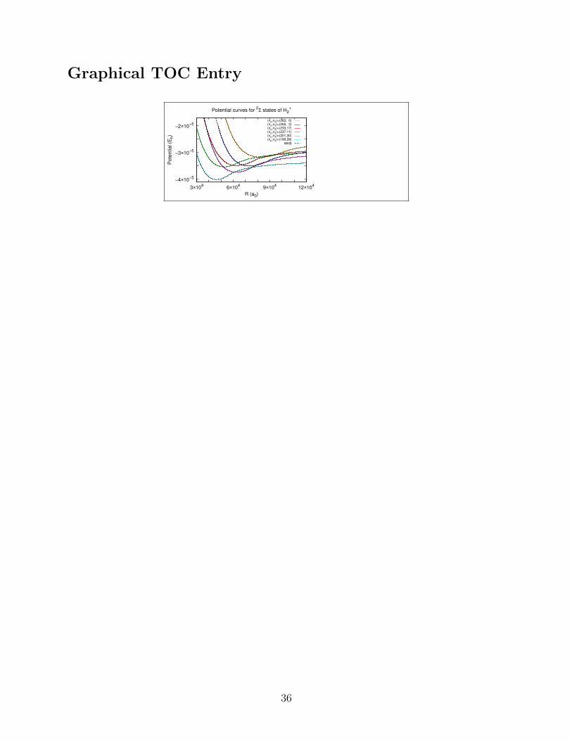
Graphical TOC Entry

−4×10−5

−3×10−5

−2×10−5

3×104

6×104

9×104

12×104

Po

ten

tia

l (E

h)

R (a0)

Potential curves for 2Σ states of H2

+

(nη,nξ)=(283, 0)(nη,nξ)=(265, 2)(nη,nξ)=(233,17)(nη,nξ)=(237,11)(nη,nξ)=(201,30)(nη,nξ)=(189,28)

WKB

36