Section 2: Quantum Mechanics as a QFT Feynman rules …web.mit.edu/8.323/sp12/Lecture notes and...

QM reviewCorrelation Functions

Interactions and Feynman Diagrams

Physics 8.323

Section 2:

Quantum Mechanics as a QFT

Feynman rules for non-relativistic QM perturbation theory

(A rough road map for QFT)

February 2012

c©2012 W. Taylor 8.323 Section 2: QM as QFT 1 / 27



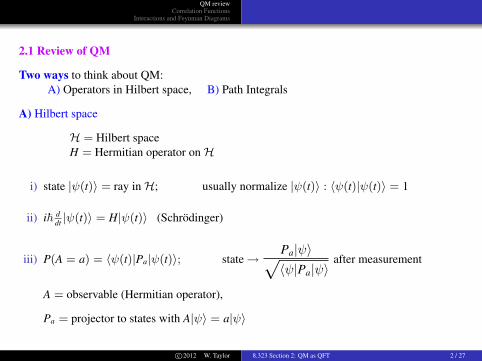
2.1 Review of QM

Two ways to think about QM:A) Operators in Hilbert space, B) Path Integrals

A) Hilbert space

H = Hilbert spaceH = Hermitian operator on H

i) state |ψ(t)〉 = ray in H; usually normalize |ψ(t)〉 : 〈ψ(t)|ψ(t)〉 = 1

ii) i~ ddt |ψ(t)〉 = H|ψ(t)〉 (Schrodinger)

iii) P(A = a) = 〈ψ(t)|Pa|ψ(t)〉; state →Pa|ψ〉√〈ψ|Pa|ψ〉

after measurement

A = observable (Hermitian operator),

Pa = projector to states with A|ψ〉 = a|ψ〉




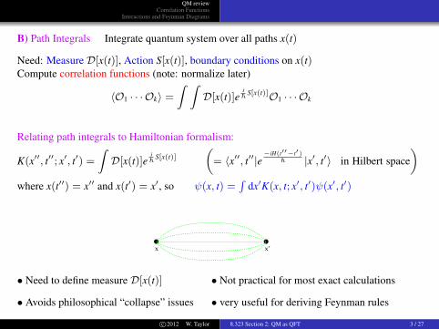
B) Path Integrals Integrate quantum system over all paths x(t)

Need: Measure D[x(t)], Action S[x(t)], boundary conditions on x(t)Compute correlation functions (note: normalize later)

〈O1 · · · Ok〉 =

Z ZD[x(t)]e

i~ S[x(t)]O1 · · · Ok

Relating path integrals to Hamiltonian formalism:

K(x′′, t′′; x′, t′) =

ZD[x(t)]e

i~ S[x(t)]

„= 〈x′′, t′′|e

−iH(t′′−t′)~ |x′, t′〉 in Hilbert space

«where x(t′′) = x′′ and x(t′) = x′, so ψ(x, t) =

Rdx′K(x, t; x′, t′)ψ(x′, t′)

x x’

• Need to define measure D[x(t)] • Not practical for most exact calculations

• Avoids philosophical “collapse” issues • very useful for deriving Feynman rules




The Simple Harmonic Oscillator (SHO) in Hilbert space and path integral languages

A)H =

p2

2[m]+

[m]ω2

2x2, p = −i[~]

∂

∂x

(we set m = ~ = c = 1). Define

a =

rω

2(x +

ipω

), a† =

rω

2(x− ip

ω)

a, a† commute as lowering and raising operators:

[a, a†] = 1; H = [~]ω(a†a +12)

Eigenstates |n〉:• H|n〉 = ω(n + 1/2)|n〉• a|n〉 =

√n|n− 1〉, a†|n〉 =

√n + 1|n + 1〉; (a|0〉 = 0)

a|0〉 = 0 ⇒ 〈x|0〉 = 4rω

πe−

ω2 x2, . . .




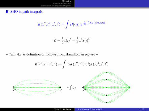
B) SHO in path integrals

K(x′′, t′′; x′, t′) =

ZD[x(t)]e

i[~]

RdtL(x(t),x(t))

L =12

x(t)2 − 12ω2x(t)2

– Can take as definition or follows from Hamiltonian picture +

K(x′′, t′′; x′, t′) =

ZdyK(x′′, t′′; y, t)K(y, t; x′, t′)

x’’ x’’x’ x’= dy




2.2 Correlation Functions in Quantum Mechanics

Treat QM as a (0 + 1)-dimensional QFT

Do perturbative quantum mechanics calculations from point of view of QFT.

Remember, you know the physics!— Same results as standard perturbation theory, different calculation method.

All calculations → finite answers.

Refer back later when we do (3+1)-dimensional QFT

Compute: N-point functions (“correlation functions”)

〈x(tN)x(tN−1) · · · x(t1)〉

Example: 2-point function (“propagator”) in ground state

〈x(t2)x(t1)〉0




A) Heisenberg picture: x(t) = eiHtxe−iHt,

states fixed.〈x(t2)x(t1)〉0 = 〈0|eiHt2 xe−iH(t2−t1)xe−iHt1 |0〉

wherex =

1√2ω

(a + a†)

Time Ordering

Ordering: correct when t2 > t1

Define

T (x(t2)x(t1)) =

x(t2)x(t1), t2 > t1

x(t1)x(t2), t1 > t2

“Time-ordered” 2-point function is

D(t2, t1) = 〈T (x(t2)x(t1))〉0

= 〈0| 1√2ω

a e−iω|t2−t1| 1√2ω

a†|0〉= 12ω

e−iω|t2−t1|




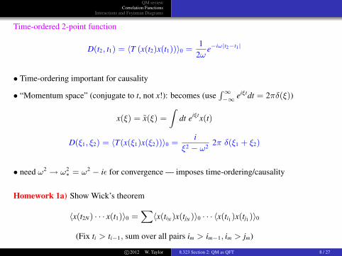
Time-ordered 2-point function

D(t2, t1) = 〈T (x(t2)x(t1))〉0 =1

2ωe−iω|t2−t1|

• Time-ordering important for causality

• “Momentum space” (conjugate to t, not x!): becomes (useR∞−∞ eiξtdt = 2πδ(ξ))

x(ξ) = x(ξ) =

Zdt eiξtx(t)

D(ξ1, ξ2) = 〈T(x(ξ1)x(ξ2))〉0 =i

ξ2 − ω2 2π δ(ξ1 + ξ2)

• need ω2 → ω2∗ = ω2 − iε for convergence — imposes time-ordering/causality

Homework 1a) Show Wick’s theorem

〈x(t2N) · · · x(t1)〉0 =X

〈x(tiN )x(tjN )〉0 · · · 〈x(ti1)x(tj1)〉0

(Fix ti > ti−1, sum over all pairs im > im−1, im > jm)




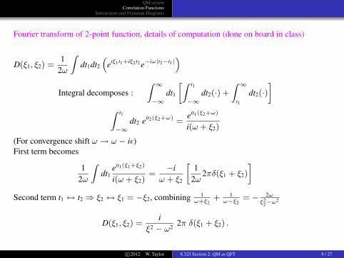
Fourier transform of 2-point function, details of computation (done on board in class)

D(ξ1, ξ2) =1

2ω

Zdt1dt2

“eiξ1t1+iξ2t2 e−iω|t2−t1|

”Integral decomposes :

Z ∞

−∞dt1

»Z t1

−∞dt2(·) +

Z ∞

t1

dt2(·)–

Z t1

−∞dt2 eit2(ξ2+ω) =

eit1(ξ2+ω)

i(ω + ξ2)

(For convergence shift ω → ω − iε)First term becomes

12ω

Zdt1

eit1(ξ1+ξ2)

i(ω + ξ2)=

−iω + ξ2

»1

2ω2πδ(ξ1 + ξ2)

–Second term t1 ↔ t2 ⇒ ξ2 ↔ ξ1 = −ξ2, combining 1

ω+ξ2+ 1

ω−ξ2= − 2ω

ξ22−ω2

D(ξ1, ξ2) =i

ξ2 − ω2 2π δ(ξ1 + ξ2) .




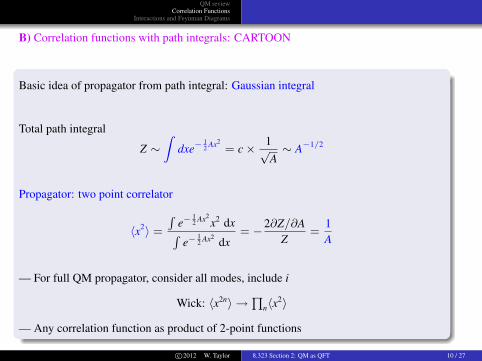
B) Correlation functions with path integrals: CARTOON

Basic idea of propagator from path integral: Gaussian integral

Total path integral

Z ∼Z

dxe−12 Ax2

= c× 1√A∼ A−1/2

Propagator: two point correlator

〈x2〉 =

Re−

12 Ax2

x2 dxRe−

12 Ax2 dx

= −2∂Z/∂AZ

=1A

— For full QM propagator, consider all modes, include i

Wick: 〈x2n〉 →Q

n〈x2〉

— Any correlation function as product of 2-point functions




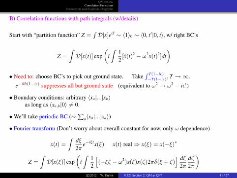
B) Correlation functions with path integrals (w/details)

Start with “partition function” Z =RD[x]eiS ∼ 〈1〉0 ∼ 〈0, t′|0, t〉, w/ right BC’s

Z =

ZD[x(t)] exp

„iZ

12[x(t)2 − ω2x(t)2]dt

«

• Need to: choose BC’s to pick out ground state. TakeR T(1−iε)−T(1−iε), T →∞.

e−iHt(1−iε) suppresses all but ground state (equivalent to ω2 → ω2 − iε′)

• Boundary conditions: arbitrary 〈xa|...|xb〉as long as 〈xa,b|0〉 6= 0.

• We’ll take periodic BC (∼P

a〈xa|...|xa〉)

• Fourier transform (Don’t worry about overall constant for now, only ω dependence)

x(t) =

Zdξ2π

e−iξtx(ξ) x(t) real ⇒ x(ξ) = x(−ξ)∗

Z =

ZD[x(ξ)] exp

„iZ

12

h(−ξζ − ω2)x(ξ)x(ζ)2πδ(ξ + ζ)

i dξ2π

dζ2π

«c©2012 W. Taylor 8.323 Section 2: QM as QFT 11 / 27



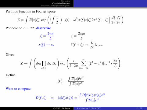
Partition function in Fourier space

Z =

ZD[x(ξ)] exp

„iZ

12

h(−ξζ − ω2)x(ξ)x(ζ)2πδ(ξ + ζ)

i dξ2π

dζ2π

«Periodic on L = 2T , discretize

ξ =2πn

Lζ =

2πmL

x(ξ) → xn δ(ξ + ζ) → L2πδn,−m

Gives

Z →Z

dx0

Yn>0

dxndxn

!exp

i

2 · 2π

∞Xm=−∞

(ξ2 − ω2)|xm|2 ·2πL

!

Define

〈F〉 =

RD[x]FeiSRD[x]eiS

Want to compute:

D(ξ, ζ) = 〈x(ξ)x(ζ)〉 =

RD[x]x(ξ)x(ζ)eiSR

D[x]eiS




Two-point function in Fourier space

D(ξ, ζ) = 〈x(ξ)x(ζ)〉 =

RD[x]x(ξ)x(ζ)eiSR

D[x]eiS

→ Dnm =

R `Qr>0 dxrdxr

´xnxm exp

`i

2π

Ps>0(ξ

2s − ω2)xsxs

2πL

´RD[x]eiS

=2πi

ξ2 − ω2

L2πδn+m,0

using

i2

Zdzdze−azz = 2π

Z ∞

0rdr e−ar2

= π/a,i2

Zdzdz zz e−azz = π/a2

We thus find in the continuous limit

D(ξ, ζ) → iξ2 − ω2 2πδ(ξ + ζ)

Treat 0-mode slightly differently (real), but irrelevant in continuum limitStructure of time-ordered propagator automatic, with ω → ω − iεOverall constant (including phase) cancels in PI quotient




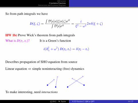
So from path integrals we have

D(ξ, ζ) =

RD[x]x(ξ)x(ζ)eiSR

D[x]eiS=

iξ2 − ω2 2πδ(ξ + ζ)

HW 1b) Prove Wick’s theorem from path integrals

What is D(t2, t1)? It is a Green’s function

i(∂2t2 + ω2) D(t2, t1) = δ(t2 − t1)

Describes propagation of SHO equation from source

Linear equation ⇒ simple noninteracting (free) dynamics

To make interesting, need interactions




2.3 Interacting Theory and Feynman Diagrams

Add interaction potential V(x); simple example: cubic perturbation

H = H0 + V(x)

= (p2

2+ω2

2x2) +

A3!

x3

Want to compute 〈x(tN)...x(t1)〉

Given by 〈Ω|x(tN)...x(t1)|Ω〉 in Schrodinger theory where

|Ω〉 = ground state of interacting theory

Note: Ground state nonperturbatively unstable — ignore instability in pert. theory

Example: 1-point function with Ax3/6 perturbation

Consider 〈x(0)〉, mean position in ground state

〈x(0)〉 is measurable physical quantity (perturbatively)

Can compute 〈x(0)〉 in 4 ways— do computation to O(A)




a) Perturbation theory in QM(nondegenerate, time-independent)

Ground state to O(A)

|Ω〉 = |0〉+Xn6=0

|n〉〈n| A

6 x3|0〉E0 − En

+ O(A2)

We then compute

〈x〉 = 〈Ω|x|Ω〉

= 2〈0|x|1〉 ·A6 〈1|x

3|0〉−ω + · · ·

[x =1√2ω

(a + a†), 〈1|a†aa†|0〉 = 1, 〈1|aa†a†|0〉 = 2]

= − A3ω

(1

2ω)2 · 3 + · · ·

= − A4ω3 + O(A2)




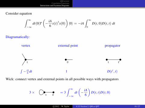
Consider equationZ ∞

−∞dt〈0|T

„− iA

6x(t)3x(0)

«|0〉 = −iA

Z ∞

0D(t, 0)D(t, t) dt

Diagramatically:

vertex external point propagator

t 0 t t’R− iA

6 dt 1 D(t′, t)

Wick: connect vertex and external points in all possible ways with propagators

3×t 0

= 3Z ∞

−∞dt„− iA

6

«D(t, t)D(t, 0)




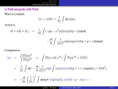
c) Path integrals with WickWant to compute

〈x〉 = 〈x(0)〉 =1

2π

Zdp〈x(p)〉

Action is

iS = i(S0 + S1) =i

4π

Z(−pq− ω2)x(p)x(q)δ(p + q)dpdq

− iA6

Z1

(2π)2 x(p)x(q)x(r)δ(p + q + r)dpdqdr

Computation

〈x〉 =

RD[x]xeiSRD[x]eiS

=

ZD[x] x iS1 eiS0/

ZD[x]eiS0 +O(S2

1)

=1

2π

Zdp〈 − iA

61

(2π)2 x(p)

Zx(q)x(r)x(s)δ(q + r + s)dqdrds〉0 + O(A2)

= − iA4π

„1

2π

«2 Zdpdqdr 〈x(p)x(q)〉0 〈x(r)x(−q− r)〉0+ · · ·




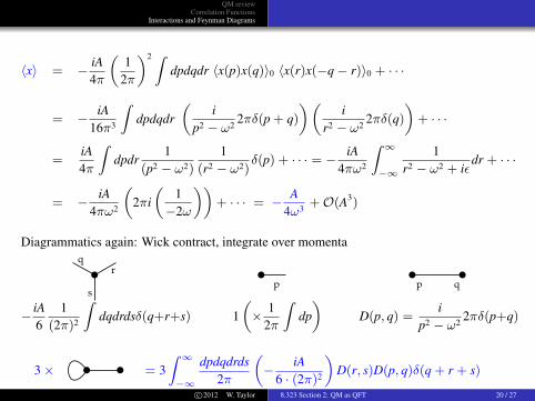
〈x〉 = − iA4π

„1

2π

«2 Zdpdqdr 〈x(p)x(q)〉0 〈x(r)x(−q− r)〉0 + · · ·

= − iA16π3

Zdpdqdr

„i

p2 − ω2 2πδ(p + q)

«„i

r2 − ω2 2πδ(q)

«+ · · ·

=iA4π

Zdpdr

1(p2 − ω2)

1(r2 − ω2)

δ(p) + · · · = − iA4πω2

Z ∞

−∞

1r2 − ω2 + iε

dr + · · ·

= − iA4πω2

„2πi„

1−2ω

««+ · · · = − A

4ω3 +O(A3)

Diagrammatics again: Wick contract, integrate over momenta

r

q

sp p q

− iA6

1(2π)2

Zdqdrdsδ(q+r+s) 1

„× 1

2π

Zdp«

D(p, q) =i

p2 − ω2 2πδ(p+q)

3× = 3Z ∞

−∞

dpdqdrds2π

„− iA

6 · (2π)2

«D(r, s)D(p, q)δ(q + r + s)




General diagrammatics:

An contribution to 〈x(tm)...x(t1)〉

m external vertices rrr qqq1

2

m

rrrJJ

JJ

JJ

qqqn internal vertices

labeled, even if ti = tj1n! from e−iV , − iA

3! for each vertex.

Wick: connect in all ways

Example: n = 2,m = 2

7!! = 105 diagrams, each × 12!3!3! = 1

72

+ + +...

shortcut: consider only topologically distinct diagramsc©2012 W. Taylor 8.323 Section 2: QM as QFT 21 / 27



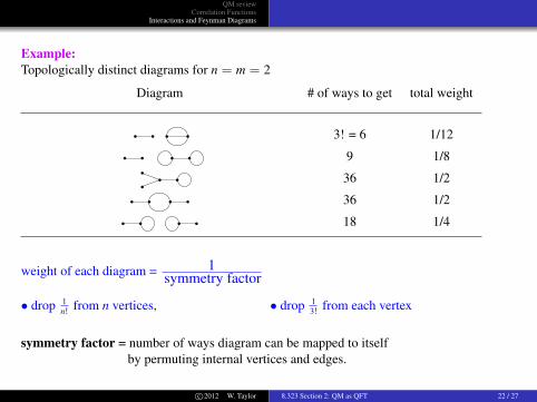
Example:Topologically distinct diagrams for n = m = 2

Diagram # of ways to get total weight

3! = 6 1/12

9 1/8

36 1/2

36 1/2

18 1/4

weight of each diagram = 1symmetry factor

• drop 1n! from n vertices, • drop 1

3! from each vertex

symmetry factor = number of ways diagram can be mapped to itselfby permuting internal vertices and edges.




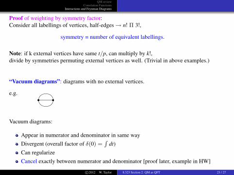
Proof of weighting by symmetry factor:Consider all labellings of vertices, half-edges → n! Π 3!,

symmetry = number of equivalent labellings.

Note: if k external vertices have same t/p, can multiply by k!,divide by symmetries permuting external vertices as well. (Trivial in above examples.)

“Vacuum diagrams”: diagrams with no external vertices.

e.g.

Vacuum diagrams:

Appear in numerator and denominator in same wayDivergent (overall factor of δ(0) =

Rdt)

Can regularizeCancel exactly between numerator and denominator [proof later, example in HW]




4th approach to computing N-pt. funs:

d) Diagrammatics

Build all topologically distinct non-vacuum diagrams

m external vertices

rrr qqqrrrJJ

JJ

JJ

qqq n internal vertices

connected in all topologically distinct ways

correlation function =X

diagrams

vertices× propagatorssymmetry factor




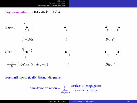
Feynman rules for QM with V = Ax3/6

x spacet 0 t t’

R−iAdt 1 D(t, t′)

p space r

q

sp p q

− iA(2π)2

Rdpdqdr δ(p + q + r) 1 D(p, p′)

Form all topologically distinct diagrams


diagrams





Form all topologically distinct diagrams


diagrams


• integrate over internal t, p ⇒ 〈x(tN)...x(t1)〉 or 〈x(pN)...x(p1)〉

• momentum space: overall 2πδ(p1 + ...+ pn),R dp

2πfor internal (“loop”) momenta.

Example:

〈x(0)〉 ⇒ 12 t 0

=−iA

2

ZdtD(t, t)D(t, 0) =

−A4ω3




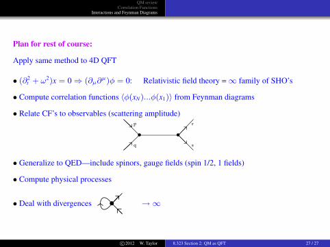
Plan for rest of course:

Apply same method to 4D QFT

• (∂2t + ω2)x = 0 ⇒ (∂µ∂

µ)φ = 0: Relativistic field theory = ∞ family of SHO’s

• Compute correlation functions 〈φ(xN)...φ(x1)〉 from Feynman diagrams

• Relate CF’s to observables (scattering amplitude)p

q

r

s

• Generalize to QED—include spinors, gauge fields (spin 1/2, 1 fields)

• Compute physical processes

• Deal with divergences →∞


Section 2: Quantum Mechanics as a QFT Feynman rules …web.mit.edu/8.323/sp12/Lecture notes and...

Documents

Transcript of Section 2: Quantum Mechanics as a QFT Feynman rules …web.mit.edu/8.323/sp12/Lecture notes and...