Second Order Backward Stochastic Differential Equations and

Fully Non-Linear Parabolic PDEs

Patrick Cheridito ∗ H. Mete Soner † Nizar Touzi ‡ Nicolas Victoir §

March 22, 2006

Abstract

For a d-dimensional diffusion of the form dXt = µ(Xt)dt+ σ(Xt)dWt, and continuousfunctions f and g, we study the existence and uniqueness of adapted processes Y , Z,Γ and A solving the second order backward stochastic differential equation (2BSDE)

dYt = f(t,Xt, Yt, Zt,Γt) dt+ Z ′t dXt , t ∈ [0, T ) ,

dZt = At dt+ Γt dXt , t ∈ [0, T ) ,

YT = g(XT ) .

If the associated PDE

−vt(t, x) + f(t, x, v(t, x), Dv(t, x), D2v(t, x)) = 0 , (t, x) ∈ [0, T )× Rd ,

v(T, x) = g(x) ,

has a sufficiently regular solution, then it follows directly from Ito’s formula that theprocesses

v(t,Xt), Dv(t,Xt), D2v(t,Xt), LDv(t,Xt) , t ∈ [0, T ] ,

solve the 2BSDE, where L is the Dynkin operator of X without the drift term.The main result of the paper shows that if f is Lipschitz in Y as well as decreasing

in Γ and the PDE satisfies a comparison principle as in the theory of viscosity solutions,then the existence of a solution (Y,Z,Γ, A) to the 2BSDE implies that the associatedPDE has a unique continuous viscosity solution v and the process Y is of the formYt = v(t,Xt), t ∈ [0, T ]. In particular, the 2BSDE has at most one solution. Thisprovides a stochastic representation for solutions of fully non-linear parabolic PDEs.As a consequence, the numerical treatment of such PDE’s can now be approached byMonte Carlo methods.

Key Words: Second order backward stochastic differential equations, Fully non-linearparabolic partial differential equations, Viscosity solutions, Monte Carlo methods.

AMS 2000 Subject Classification: 60H30, 35K55, 60H35, 65C05.

∗Princeton University, Princeton, USA, dito@princeton.edu.†Koc University, Istanbul, Turkey, msoner@ku.edu.tr. Member of the Turkish Academy of Sciences and

this work was partly supported by the Turkish Academy of Sciences.‡CREST, Paris, France, touzi@ensae.fr, and Tanaka Business School, Imperial College London, England,

n.touzi@imperial.ac.uk.§Oxford University, Oxford, England, victoir@gmail.com.

1

1 Introduction

Since their introduction, backward stochastic differential equations (BSDEs) have receivedconsiderable attention in the probability literature. Interesting connections to partial dif-ferential equations (PDEs) have been obtained, and the theory has found wide applicationsin areas like stochastic control, theoretical economics and mathematical finance.

BSDEs were introduced by Bismut [7] in the linear case and by Pardoux and Peng [39]in the general case. According to these authors, a solution to a BSDE consists of a pair ofadapted processes (Y, Z) taking values in Rn and Rd×n, respectively, such that

dYt = f(t, Yt, Zt)dt+ Z ′tdWt , t ∈ [0, T ) ,

YT = ξ ,(1.1)

where T is a finite time horizon, (Wt)t∈[0,T ] a d-dimensional Brownian motion on a filteredprobability space (Ω,F , (Ft)t∈[0,T ], P ), f a progressively measurable function from Ω ×[0, T ]× Rn × Rd×n to Rn and ξ an Rn-valued, FT -measurable random variable.

The key feature of BSDEs is the random terminal condition ξ that the solution is requiredto satisfy. Due to the adaptedness requirement on the processes Y and Z, this conditionposes certain difficulties in the stochastic setting. But they have been overcome, andnow an impressive theory is available; see for instance, Bismut [7, 8], Arkin and Saksonov[2], Pardoux and Peng [39, 40, 41], Peng [43, 44, 45, 46, 47, 48], Antonelli [1], Ma et al.[36, 37, 38], Douglas et al. [22], Cvitanic et al. [17, 18, 19], Chevance [15], Pardoux andTang [42], Delarue [20], Bouchard and Touzi [9], Delarue and Menozzi [21], or the overviewpaper El Karoui et al. [23].

If the randomness in the parameters f and ξ in (1.1) is coming from the state of aforward SDE, then the BSDE is referred to as a forward-backward stochastic differentialequation (FBSDE) and its solution can be written as a deterministic function of timeand the state process. Under suitable regularity assumptions, this function can be shownto be the solution of a parabolic PDE. FBSDEs are called uncoupled if the solution ofthe BSDE does not enter the dynamics of the forward SDE and coupled if it does. Thecorresponding parabolic PDE is semi-linear in case the FBSDE is uncoupled and quasi-linear if the FBSDE is coupled; see Peng [44, 46], Pardoux and Peng [40], Antonelli [1], Maet al. [36, 37], Pardoux and Tang [42]. These connections between FBSDEs and PDEs haveled to interesting stochastic representation results for solutions of semi-linear and quasi-linear parabolic PDEs, generalizing the Feynman–Kac representation of linear parabolicPDEs and opening the way to Monte Carlo methods for the numerical treatment of suchPDEs, see for instance, Zhang [52], Bally and Pages [3], Ma et al. [36, 37, 38], Bouchard andTouzi [9], Delarue and Menozzi [21]. However, PDEs corresponding to standard FBSDEscannot be non-linear in the second order derivatives because second order terms only ariselinearly through Ito’s formula from the quadratic variation of the underlying state process.

In this paper we introduce FBSDEs with second order dependence in the generator f . Wecall them second order backward stochastic differential equations (2BSDEs) and show howthey are related to fully non-linear parabolic PDEs. This extends the range of connectionsbetween stochastic equations and PDEs. In particular, it opens the way for the development

2

of Monte Carlo methods for the numerical solution of fully non-linear parabolic PDEs. Ourapproach is motivated by results in Cheridito et al. [13, 14], which show how second ordertrading constraints lead to fully non-linear parabolic Hamilton–Jacobi–Bellman equationsfor the super-replication cost of European contingent claims.

The structure of the paper is as follows: In Section 2, we explain the notation andintroduce 2BSDEs together with their associated PDEs. In Section 3, we show that theexistence of a sufficiently regular solution to the associated PDE implies the existence of asolution to the 2BSDE. Our main result, Theorem 4.10 in Section 4, shows the converse: Ifthe PDE satisfies suitable Lipschitz and parabolicity conditions together with a comparisonprinciple from the theory of viscosity solutions, then the existence of a solution to the2BSDE implies that the PDE has a unique continuous viscosity solution v. Moreover,the solution of the 2BSDE can then be written in terms of v and the underlying stateprocess. This implies that the solution of the 2BSDE is unique, and it provides a stochasticrepresentation result for fully non-linear parabolic PDEs. In Section 5 we discuss MonteCarlo schemes for the numerical solution of such PDEs. In Section 6 we show how theresults of the paper can be adjusted to the case of PDEs with boundary conditions.

2 Notation and definitions

Let d ≥ 1 be a natural number. By Md we denote the set of all d × d matrices withreal components. B′ is the transpose of a matrix B ∈ Md and Tr[B] its trace. By Md

inv

we denote the set of all invertible matrices in Md, by Sd all symmetric matrices in Md,and by Sd+ all positive semi-definite matrices in Md. For B,C ∈ Md, we write B ≥ C ifB − C ∈ Sd+. For x ∈ Rd, we set

|x| :=√x2

1 + · · ·+ x2d

and for B ∈Md,

|B| :=

√√√√ d∑i,j=1

B2ij .

Equalities and inequalities between random variables are always understood in the almostsure sense. We fix a finite time horizon T ∈ (0,∞) and let (Wt)t∈[0,T ] be a d-dimensionalBrownian motion on a complete probability space (Ω,F , P ). For s ∈ [0, T ], we set W s

t :=Wt −Ws, t ∈ [s, T ] and denote by Fs,T = (Fs

t )t∈[s,T ] the augmented filtration generated by(W s

t )t∈[s,T ].µ : Rd → Rd and σ : Rd → Md

inv are assumed to be functions satisfying the followingLipschitz and growth conditions: There exists a constant K with

|µ(x)− µ(y)|+ |σ(x)− σ(y)| ≤ K|x− y| for all x, y ∈ Rd , (2.1)

and a constant p1 ∈ [0, 1] such that

|µ(x)|+ |σ(x)| ≤ K(1 + |x|p1) for all x ∈ Rd . (2.2)

3

Then, for every initial condition (s, x) ∈ [0, T ]× Rd, the forward SDE

dXt = µ(Xt)dt+ σ(Xt)dWt , t ∈ [s, T ] ,

Xs = x ,(2.3)

has a unique strong solution (Xs,xt )t∈[s,T ]; see for instance, Theorem 5.2.9 in Karatzas and

Shreve [30]. Note that for existence and uniqueness of a strong solution to the SDE (2.3),p1 = 1 in condition (2.2) is enough. But for p1 ∈ [0, 1), we will get a better growth exponentp in Proposition 4.5 below. In any case, the process (Xs,x

t )t∈[s,T ] is adapted to the filtrationFs,T , and by Ito’s formula, we have for all ϕ ∈ C1,2([s, T ]× Rd) and t ∈ [s, T ],

ϕ (t,Xs,xt ) = ϕ(s, x) +

∫ t

sLϕ (r,Xs,x

r ) dr +∫ t

sDϕ (r,Xs,x

r )′ dXs,xr , (2.4)

where

Lϕ(t, x) = ϕt(t, x) +12Tr[D2ϕ(t, x)σ(x)σ(x)′] ,

and Dϕ, D2ϕ are the gradient and the matrix of second derivatives of ϕ with respect tothe x-variables.

In the whole paper, f : [0, T ) × Rd × R × Rd × Sd → R and g : Rd → R are continuousfunctions.

Definition 2.1 Let (s, x) ∈ [0, T ) × Rd and (Yt, Zt,Γt, At)t∈[s,T ] a quadruple of Fs,T -progressively measurable processes taking values in R, Rd, Sd and Rd, respectively. Thenwe call (Y, Z,Γ, A) a solution of the second order backward stochastic differential equation(2BSDE) corresponding to (Xs,x, f, g) if

dYt = f(t,Xs,xt , Yt, Zt,Γt) dt+ Z ′t dX

s,xt , t ∈ [s, T ) , (2.5)

dZt = At dt+ Γt dXs,xt , t ∈ [s, T ) , (2.6)

YT = g(Xs,xT

), (2.7)

where Z ′t dXs,xt denotes Fisk–Stratonovich integration, which is related to Ito integration

by

Z ′t dXs,xt = Z ′t dX

s,xt +

12d 〈Z,Xs,x〉t = Z ′t dX

s,xt +

12

Tr[Γt σ(Xs,xt )σ(Xs,x

t )′] dt . (2.8)

The equations (2.5)–(2.7) can be viewed as a whole family of 2BSDEs indexed by (s, x) ∈[0, T )×Rd. In the following sections, we will show relations between this family of 2BSDEsand the associated PDE

−vt(t, x) + f(t, x, v(t, x), Dv(t, x), D2v(t, x)

)= 0 on [0, T )× Rd , (2.9)

with terminal condition

v(T, x) = g(x) , x ∈ R . (2.10)

4

Since Z is a semimartingale, the use of the Fisk–Stratonovich integral in (2.5) means noloss of generality, but it simplifies the notation in the PDE (2.9). Alternatively, (2.5) couldbe written in terms of the Ito integral as

dYt = f (t,Xs,xt , Yt, Zt,Γt) dt+ Z ′t dX

s,xt (2.11)

for

f(t, x, y, z, γ) = f(t, x, y, z, γ) +12

Tr[γ σ(x)σ(x)′

].

In terms of f , the PDE (2.9) reads as follows:

−vt(t, x) + f(t, x, v(t, x), Dv(t, x), D2v(t, x))− 12Tr[D2v(t, x)σ(x)σ(x)′] = 0 .

Note that the form of the PDE (2.9) does not depend on the functions µ and σ determiningthe dynamics in (2.3). So, we could restrict our attention to the case where µ ≡ 0 andσ ≡ Id, the d× d identity matrix. But the freedom to choose µ and σ from a more generalclass provides additional flexibility in the design of the Monte Carlo schemes discussed inSection 5 below.

3 From a solution of the PDE to a solution of the 2BSDE

Assume v : [0, T ]× Rd → R is a continuous function such that

vt, Dv,D2v,LDv exist and are continuous on [0, T )× Rd ,

and v solves the PDE (2.9) with terminal condition (2.10). Then it follows directly fromIto’s formula (2.4) that for each pair (s, x) ∈ [0, T )× Rd, the processes

Yt = v (t,Xs,xt ) , t ∈ [s, T ] ,

Zt = Dv (t,Xs,xt ) , t ∈ [s, T ] ,

Γt = D2v (t,Xs,xt ) , t ∈ [s, T ] ,

At = LDv (t,Xs,xt ) , t ∈ [s, T ] ,

solve the 2BSDE corresponding to (Xs,x, f, g).

4 From a solution of the 2BSDE to a solution of the PDE

In all of Section 4 we assume that

f : [0, T )× Rd × R× Rd × Sd → R and g : Rd → R

are continuous functions that satisfy the following Lipschitz and growth assumptions:(A1) For every N ≥ 1 there exists a constant FN such that

|f(t, x, y, z, γ)− f(t, x, y, z, γ)| ≤ FN |y − y|

5

for all (t, x, y, y, z, γ) ∈ [0, T )× Rd × R2 × Rd × Sd with max |x| , |y| , |y| , |z| , |γ| ≤ N .(A2) There exist constants F and p2 ≥ 0 such that

|f(t, x, y, z, γ)| ≤ F (1 + |x|p2 + |y|+ |z|p2 + |γ|p2)

for all (t, x, y, z, γ) ∈ [0, T )× Rd × R× Rd × Sd.(A3) There exist constants G and p3 ≥ 0 such that

|g(x)| ≤ G(1 + |x|p3) for all x ∈ Rd .

4.1 Admissible strategies

We fix constants p4, p5 ≥ 0 and denote for all (s, x) ∈ [0, T ] × Rd and m ≥ 0 by As,xm theclass of all processes of the form

Zt = z +∫ t

sArdr +

∫ t

sΓrdXs,x

r , t ∈ [s, T ] ,

where z ∈ Rd, (At)t∈[s,T ] is an Rd-valued, Fs,T -progressively measurable process, (Γt)t∈[s,T ]

is an Sd-valued, Fs,T -progressively measurable process such that

max |Zt| , |At| , |Γt| ≤ m(1 + |Xs,xt |p4) for all t ∈ [s, T ] , (4.1)

and

|Γr − Γt| ≤ m(1 + |Xs,xr |p5 + |Xs,x

t |p5)(|r − t|+ |Xs,xr −Xs,x

t |) for all r, t ∈ [s, T ] . (4.2)

Set As,x :=⋃m≥0A

s,xm . It follows from the assumptions (A1) and (A2) on f and condition

(4.1) on Z that for all y ∈ R and Z ∈ As,x, the forward SDE

dYt = f(t,Xs,xt , Yt, Zt,Γt) dt+ Z ′t dX

s,xt , t ∈ [s, T ) , (4.3)

Ys = y , (4.4)

has a unique strong solution(Y s,x,y,Zt

)t∈[s,T ]

(this can, for instance, be shown with the

arguments in the proofs of Theorems 2.3, 2.4 and 3.1 in Chapter IV of Ikeda and Watanabe[28]).

4.2 Auxiliary stochastic target problems

For every m ≥ 0, we define the functions V m, Um : [0, T ]× Rd → R as follows:

V m(s, x) := infy ∈ R : Y s,x,y,ZT ≥ g(Xs,x

T ) for some Z ∈ As,xm ,

and

Um(s, x) := supy ∈ R : Y s,x,y,ZT ≤ g(Xs,x

T ) for some Z ∈ As,xm .

Notice that these problems do not fit into the class of stochastic target problems studiedby Soner and Touzi [49] and are more in the spirit of Cheridito et al. [13, 14].

6

Lemma 4.1 (Dynamic Programming Principle)Let (s, x,m) ∈ [0, T )× Rd × R+ and (y, Z) ∈ R×As,xm such that Y s,x,y,Z

T ≥ g(Xs,xT ). Then

Y s,x,y,Zt ≥ V m(t,Xs,x

t ) for all t ∈ (s, T ) .

Proof. Fix t ∈ (s, T ) and denote by Cd[s, t] the set of all continuous functions from [s, t] toRd. Since Xs,x

t and Y s,x,y,Zt are Fs

t -measurable, there exist measurable functions

ξ : Cd[s, t] → Rd and ψ : Cd[s, t] → R

such thatXs,xt = ξ(W s,t) and Y s,x,y,Z

t = ψ(W s,t) ,

where we denote W s,t := (W sr )r∈[s,t]. The process Z is of the form

Zr = z +∫ r

sAudu+

∫ r

sΓudXs,x

u , r ∈ [s, T ] ,

for z ∈ R, (Ar)r∈[s,T ] an Rd-valued, Fs,T -progressively measurable process, and (Γr)r∈[s,T ]

an Sd-valued, Fs,T -progressively measurable process. Therefore, there exist progressivelymeasurable functions (see Definition 3.5.15 in Karatzas and Shreve [30])

ζ, φ : [s, T ]× Cd[s, T ] → Rd

χ : [s, T ]× Cd[s, T ] → Sd

such that

Zr = ζ(r,W s,T ) , Ar = φ(r,W s,T ) and Γr = χ(r,W s,T ) for r ∈ [s, T ] .

With obvious notation, we define for every w ∈ Cd[s, t] the Rd-valued, Ft,T -progressivelymeasurable process (Zwr )r∈[t,T ] by

Zwr = ζ(t, w) +∫ r

tφ(u,w +W t,T )du+

∫ r

tχ(u,w +W t,T )dXt,ξ(ω)

u , r ∈ [t, T ] .

Let µ be the distribution of W s,t on Cd[s, t]. Then, Zw ∈ At,ξ(w)m for µ-almost all w ∈

Cd[s, t], and

1 = P[Y s,x,y,ZT ≥ g(Xs,x

T )]

=∫Cd[s,t]

P[Yt,ξ(w),ψ(w),Zw

T ≥ g(Xt,ξ(w)T )

]dµ(w) .

Hence, for µ-almost all w ∈ Cd[s, t], the control Zw satisfies

P[Ys,ξ(w),ψ(w),Zw

T ≥ g(Xs,ξ(w)T )

]= 1 .

This shows that ψ(w) = Yt,ξ(w),ψ(w),Zw

t ≥ V m(t, ξ(w)). In view of the definition of thefunctions ξ and ψ, this implies Y s,x,y,Z

t ≥ V m(t,Xs,xt ). 2

7

Since we have no a priori knowledge of any regularity of the functions V m and Um, weintroduce the semicontinuous envelopes as in Barles and Perthame [6]

V m∗ (t, x) := lim inf

(t,x)∈[0,T ] , (t,x)→(t,x)V m

(t, x

), (t, x) ∈ [0, T ]× Rd

andU∗m(t, x) := lim sup

(t,x)∈[0,T ] , (t,x)→(t,x)

Um(t, x

), (t, x) ∈ [0, T ]× Rd .

For s ∈ [0, T ), we also need the tighter semicontinuous envelopes

V m∗,s(t, x) := lim inf

(t,x)∈[s,T ] , (t,x)→(t,x)V m

(t, x

), (t, x) ∈ [s, T ]× Rd ,

andU∗,sm (t, x) := lim sup

(t,x)∈[s,T ] , (t,x)→(t,x)

Um(t, x

), (t, x) ∈ [s, T ]× Rd .

Note thatV m∗,s = V m

∗ and U∗,sm = U∗

m on (s, T ]× Rd ,

whereasV m∗,s ≥ V m

∗ and U∗,sm ≤ U∗

m on s × Rd .

For the theory of viscosity solutions, we refer to Crandall et al. [16] and the book ofFleming and Soner [25].

Theorem 4.2 Let m ≥ 0 and assume there exists an s ∈ [0, T ) such that V m∗,s is R-valued

on [s, T ]× Rd. Then V m∗,s is a viscosity supersolution of the PDE

−vt(t, x) + supβ∈Sd

+

f(t, x, v(t, x), Dv(t, x), D2v(t, x) + β

)= 0 on [s, T )× Rd .

Before turning to the proof of this result, let us state the corresponding claim for thevalue function Um.

Corollary 4.3 Let m ≥ 0 and assume there exists an s ∈ [0, T ) such that U∗,sm is R-valued

on [s, T ]× Rd. Then U∗,sm is a viscosity subsolution of the PDE

−vt(t, x) + infβ∈Sd

+

f(t, x, v(t, x), Dv(t, x), D2v(t, x)− β

)= 0 on [s, T )× Rd . (4.5)

Proof. Observe that for all (t, x) ∈ [s, T )× Rd,

−Um(t, x) = infy ∈ R : Y t,x,y,Z

T ≥ −g(Xt,xT ) for some Z ∈ At,xm

,

where for given (y, Z) ∈ R×At,xm , the process Y t,x,y,Z is the unique strong solution of theSDE

dYr = −f(r,Xt,xr ,−Yr,−Zr,−Γr)dr + (Zr)′ dXt,x

r , r ∈ [t, T ) ,

Yt = y .

8

Hence, it follows from Theorem 4.2 that −U∗,sm = (−Um)∗,s is a viscosity supersolution of

the PDE

−vt(t, x) − infβ∈Sd

+

f(t, x,−v(t, x),−Dv(t, x),−D2v(t, x)− β

)= 0 on [s, T )× Rd ,

which shows that U∗,sm is a viscosity subsolution of the PDE (4.5) on [s, T )× Rd. 2

Proof of Theorem 4.2 Choose (t0, x0) ∈ [s, T )× Rd and ϕ ∈ C∞([s, T )× Rd) such that

0 = (V m∗,s − ϕ)(t0, x0) = min

(t,x)∈[s,T )×Rd(V m∗,s − ϕ)(t, x) .

Let (tn, xn)n≥1 be a sequence in [s, T )×Rd such that (tn, xn) → (t0, x0) and V m(tn, xn) →V m∗,s(t0, x0). There exist positive numbers εn → 0 such that for yn = V m(tn, xn) + εn, there

exists Zn ∈ Atn,xnm with

Y nT ≥ g(Xn

T ) ,

where we denote (Xn, Y n) = (Xtn,xn , Y tn,xn,yn,Zn) and

Znr = zn +∫ r

tn

Anudu+∫ r

tn

ΓnudXnu , r ∈ [tn, T ] .

Note that for all n, Γntn is almost surely constant, and |zn|, |Γntn | ≤ m(1 + |xn|p4) by as-sumption (4.1). Hence, by passing to a subsequence, we can assume that zn → z0 ∈ Rd andΓntn → γ0 ∈ Sd. Observe that αn := yn − ϕ(tn, xn) → 0. We choose a decreasing sequenceof numbers δn ∈ (0, T − tn) such that δn → 0 and αn/δn → 0. By Lemma 4.1,

Y ntn+δn ≥ V m

(tn + δn, X

ntn+δn

),

and therefore,

Y ntn+δn − yn + αn ≥ ϕ

(tn + δn, X

ntn+δn

)− ϕ(tn, xn) ,

which, after two applications of Ito’s formula, becomes

αn +∫ tn+δn

tn

[f(r,Xnr , Y

nr , Z

nr ,Γ

nr )− ϕt(r,Xn

r )]dr

+ [zn −Dϕ(tn, xn)]′[Xntn+δn − xn]

+∫ tn+δn

tn

(∫ r

tn

[Anu − LDϕ(u,Xnu )] du

)′ dXn

r

+∫ tn+δn

tn

(∫ r

tn

[Γnu −D2ϕ(u,Xn

u )]dXn

u

)′ dXn

r ≥ 0 (4.6)

It is shown in Lemma 4.4 below that the sequence of random vectorsδ−1n

∫ tn+δntn

[f(r,Xnr , Y

nr , Z

nr ,Γ

nr )− ϕt(r,Xn

r )]drδ−1/2n [Xn

tn+δn− xn]

δ−1n

∫ tn+δntn

(∫ rtn

[Anu − LDϕ(u,Xnu )] du

)′ dXn

r

δ−1n

∫ tn+δntn

(∫ rtn

[Γnu −D2ϕ(u,Xn

u )]dXn

u

)′ dXn

r

, n ≥ 1 , (4.7)

9

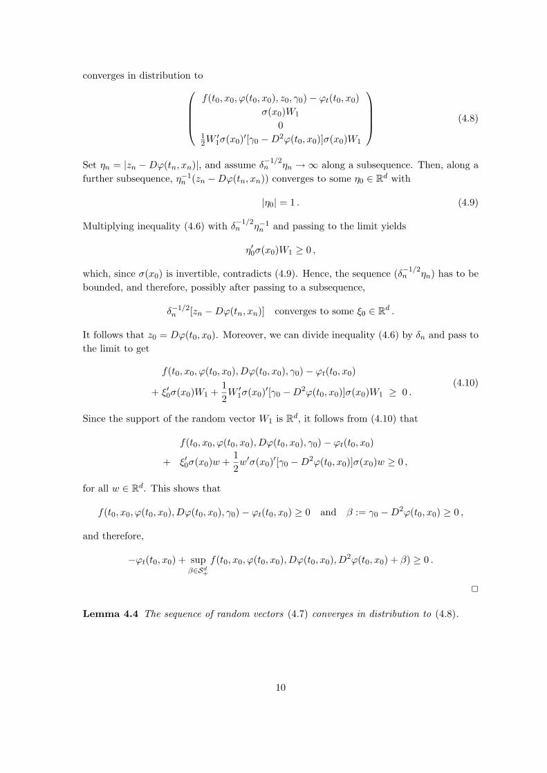
converges in distribution tof(t0, x0, ϕ(t0, x0), z0, γ0)− ϕt(t0, x0)

σ(x0)W1

012W

′1σ(x0)′[γ0 −D2ϕ(t0, x0)]σ(x0)W1

(4.8)

Set ηn = |zn −Dϕ(tn, xn)|, and assume δ−1/2n ηn →∞ along a subsequence. Then, along a

further subsequence, η−1n (zn −Dϕ(tn, xn)) converges to some η0 ∈ Rd with

|η0| = 1 . (4.9)

Multiplying inequality (4.6) with δ−1/2n η−1

n and passing to the limit yields

η′0σ(x0)W1 ≥ 0 ,

which, since σ(x0) is invertible, contradicts (4.9). Hence, the sequence (δ−1/2n ηn) has to be

bounded, and therefore, possibly after passing to a subsequence,

δ−1/2n [zn −Dϕ(tn, xn)] converges to some ξ0 ∈ Rd .

It follows that z0 = Dϕ(t0, x0). Moreover, we can divide inequality (4.6) by δn and pass tothe limit to get

f(t0, x0, ϕ(t0, x0), Dϕ(t0, x0), γ0)− ϕt(t0, x0)

+ ξ′0σ(x0)W1 +12W ′

1σ(x0)′[γ0 −D2ϕ(t0, x0)]σ(x0)W1 ≥ 0 .(4.10)

Since the support of the random vector W1 is Rd, it follows from (4.10) that

f(t0, x0, ϕ(t0, x0), Dϕ(t0, x0), γ0)− ϕt(t0, x0)

+ ξ′0σ(x0)w +12w′σ(x0)′[γ0 −D2ϕ(t0, x0)]σ(x0)w ≥ 0 ,

for all w ∈ Rd. This shows that

f(t0, x0, ϕ(t0, x0), Dϕ(t0, x0), γ0)− ϕt(t0, x0) ≥ 0 and β := γ0 −D2ϕ(t0, x0) ≥ 0 ,

and therefore,

−ϕt(t0, x0) + supβ∈Sd

+

f(t0, x0, ϕ(t0, x0), Dϕ(t0, x0), D2ϕ(t0, x0) + β) ≥ 0 .

2

Lemma 4.4 The sequence of random vectors (4.7) converges in distribution to (4.8).

10

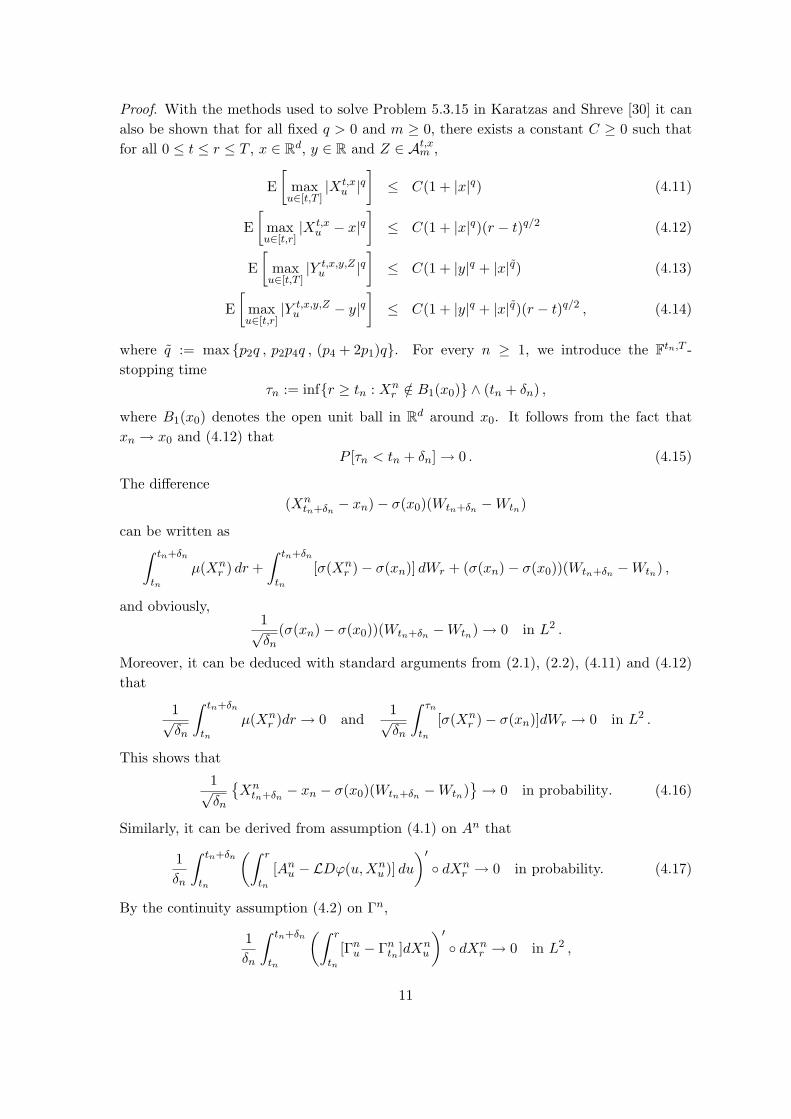
Proof. With the methods used to solve Problem 5.3.15 in Karatzas and Shreve [30] it canalso be shown that for all fixed q > 0 and m ≥ 0, there exists a constant C ≥ 0 such thatfor all 0 ≤ t ≤ r ≤ T , x ∈ Rd, y ∈ R and Z ∈ At,xm ,

E[

maxu∈[t,T ]

|Xt,xu |q

]≤ C(1 + |x|q) (4.11)

E[

maxu∈[t,r]

|Xt,xu − x|q

]≤ C(1 + |x|q)(r − t)q/2 (4.12)

E[

maxu∈[t,T ]

|Y t,x,y,Zu |q

]≤ C(1 + |y|q + |x|q) (4.13)

E[

maxu∈[t,r]

|Y t,x,y,Zu − y|q

]≤ C(1 + |y|q + |x|q)(r − t)q/2 , (4.14)

where q := max p2q , p2p4q , (p4 + 2p1)q. For every n ≥ 1, we introduce the Ftn,T -stopping time

τn := infr ≥ tn : Xnr /∈ B1(x0) ∧ (tn + δn) ,

where B1(x0) denotes the open unit ball in Rd around x0. It follows from the fact thatxn → x0 and (4.12) that

P [τn < tn + δn] → 0 . (4.15)

The difference(Xn

tn+δn − xn)− σ(x0)(Wtn+δn −Wtn)

can be written as∫ tn+δn

tn

µ(Xnr ) dr +

∫ tn+δn

tn

[σ(Xnr )− σ(xn)] dWr + (σ(xn)− σ(x0))(Wtn+δn −Wtn) ,

and obviously,1√δn

(σ(xn)− σ(x0))(Wtn+δn −Wtn) → 0 in L2 .

Moreover, it can be deduced with standard arguments from (2.1), (2.2), (4.11) and (4.12)that

1√δn

∫ tn+δn

tn

µ(Xnr )dr → 0 and

1√δn

∫ τn

tn

[σ(Xnr )− σ(xn)]dWr → 0 in L2 .

This shows that

1√δn

Xntn+δn − xn − σ(x0)(Wtn+δn −Wtn)

→ 0 in probability. (4.16)

Similarly, it can be derived from assumption (4.1) on An that

1δn

∫ tn+δn

tn

(∫ r

tn

[Anu − LDϕ(u,Xnu )] du

)′ dXn

r → 0 in probability. (4.17)

By the continuity assumption (4.2) on Γn,

1δn

∫ tn+δn

tn

(∫ r

tn

[Γnu − Γntn ]dXnu

)′ dXn

r → 0 in L2 ,

11

and

1δn

∫ tn+δn

tn

(∫ r

tn

ΓntndXnu

)′ dXn

r

−12(Wtn+δn −Wtn)′σ(x0)′γ0σ(x0)(Wtn+δn −Wtn)

→ 0 in probability.

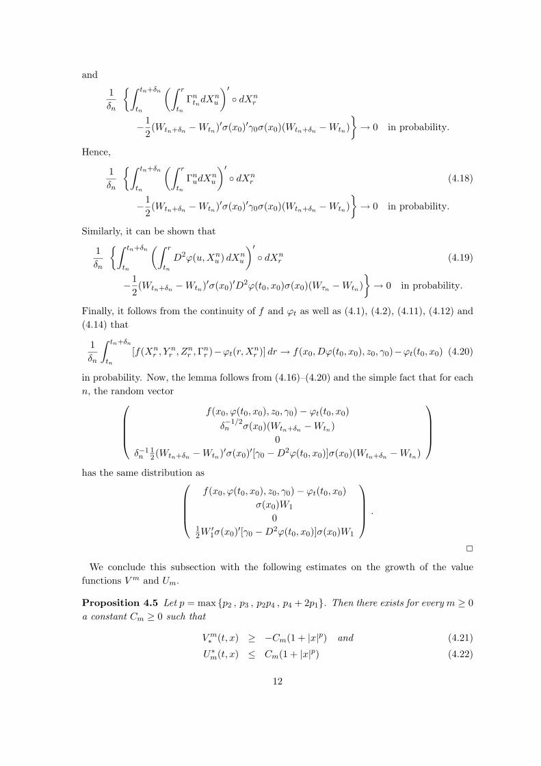
Hence,

1δn

∫ tn+δn

tn

(∫ r

tn

ΓnudXnu

)′ dXn

r (4.18)

−12(Wtn+δn −Wtn)′σ(x0)′γ0σ(x0)(Wtn+δn −Wtn)

→ 0 in probability.

Similarly, it can be shown that

1δn

∫ tn+δn

tn

(∫ r

tn

D2ϕ(u,Xnu ) dXn

u

)′ dXn

r (4.19)

−12(Wtn+δn −Wtn)′σ(x0)′D2ϕ(t0, x0)σ(x0)(Wτn −Wtn)

→ 0 in probability.

Finally, it follows from the continuity of f and ϕt as well as (4.1), (4.2), (4.11), (4.12) and(4.14) that

1δn

∫ tn+δn

tn

[f(Xnr , Y

nr , Z

nr ,Γ

nr )−ϕt(r,Xn

r )] dr → f(x0, Dϕ(t0, x0), z0, γ0)−ϕt(t0, x0) (4.20)

in probability. Now, the lemma follows from (4.16)–(4.20) and the simple fact that for eachn, the random vector

f(x0, ϕ(t0, x0), z0, γ0)− ϕt(t0, x0)δ−1/2n σ(x0)(Wtn+δn −Wtn)

0δ−1n

12(Wtn+δn −Wtn)′σ(x0)′[γ0 −D2ϕ(t0, x0)]σ(x0)(Wtn+δn −Wtn)

has the same distribution as

f(x0, ϕ(t0, x0), z0, γ0)− ϕt(t0, x0)σ(x0)W1

012W

′1σ(x0)′[γ0 −D2ϕ(t0, x0)]σ(x0)W1

.

2

We conclude this subsection with the following estimates on the growth of the valuefunctions V m and Um.

Proposition 4.5 Let p = max p2 , p3 , p2p4 , p4 + 2p1. Then there exists for every m ≥ 0a constant Cm ≥ 0 such that

V m∗ (t, x) ≥ −Cm(1 + |x|p) and (4.21)

U∗m(t, x) ≤ Cm(1 + |x|p) (4.22)

12

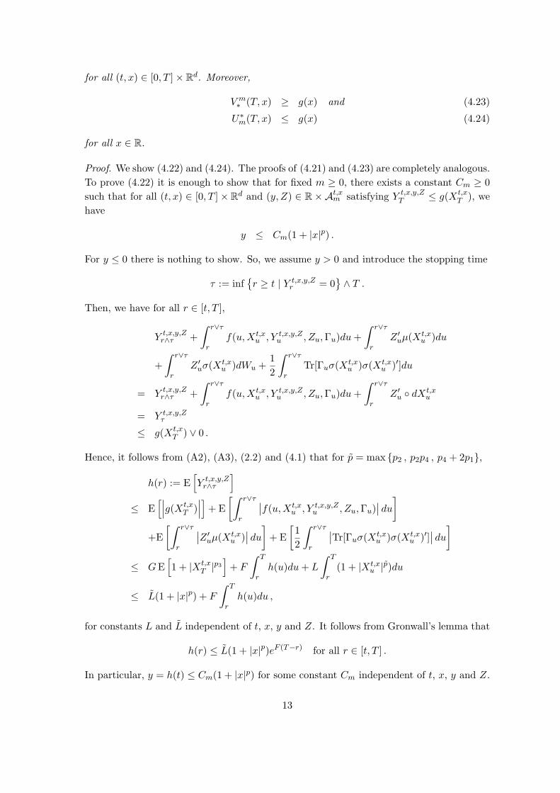
for all (t, x) ∈ [0, T ]× Rd. Moreover,

V m∗ (T, x) ≥ g(x) and (4.23)

U∗m(T, x) ≤ g(x) (4.24)

for all x ∈ R.

Proof. We show (4.22) and (4.24). The proofs of (4.21) and (4.23) are completely analogous.To prove (4.22) it is enough to show that for fixed m ≥ 0, there exists a constant Cm ≥ 0such that for all (t, x) ∈ [0, T ]× Rd and (y, Z) ∈ R×At,xm satisfying Y t,x,y,Z

T ≤ g(Xt,xT ), we

have

y ≤ Cm(1 + |x|p) .

For y ≤ 0 there is nothing to show. So, we assume y > 0 and introduce the stopping time

τ := infr ≥ t | Y t,x,y,Z

r = 0∧ T .

Then, we have for all r ∈ [t, T ],

Y t,x,y,Zr∧τ +

∫ r∨τ

rf(u,Xt,x

u , Y t,x,y,Zu , Zu,Γu)du+

∫ r∨τ

rZ ′uµ(Xt,x

u )du

+∫ r∨τ

rZ ′uσ(Xt,x

u )dWu +12

∫ r∨τ

rTr[Γuσ(Xt,x

u )σ(Xt,xu )′]du

= Y t,x,y,Zr∧τ +

∫ r∨τ

rf(u,Xt,x

u , Y t,x,y,Zu , Zu,Γu)du+

∫ r∨τ

rZ ′u dXt,x

u

= Y t,x,y,Zτ

≤ g(Xt,xT ) ∨ 0 .

Hence, it follows from (A2), (A3), (2.2) and (4.1) that for p = max p2 , p2p4 , p4 + 2p1,

h(r) := E[Y t,x,y,Zr∧τ

]≤ E

[∣∣∣g(Xt,xT )

∣∣∣] + E[∫ r∨τ

r

∣∣f(u,Xt,xu , Y t,x,y,Z

u , Zu,Γu)∣∣ du]

+E[∫ r∨τ

r

∣∣Z ′uµ(Xt,xu )

∣∣ du] + E[12

∫ r∨τ

r

∣∣Tr[Γuσ(Xt,xu )σ(Xt,x

u )′]∣∣ du]

≤ GE[1 + |Xt,x

T |p3]

+ F

∫ T

rh(u)du+ L

∫ T

r(1 + |Xt,x

u |p)du

≤ L(1 + |x|p) + F

∫ T

rh(u)du ,

for constants L and L independent of t, x, y and Z. It follows from Gronwall’s lemma that

h(r) ≤ L(1 + |x|p)eF (T−r) for all r ∈ [t, T ] .

In particular, y = h(t) ≤ Cm(1 + |x|p) for some constant Cm independent of t, x, y and Z.

13

To prove (4.24), we assume by way of contradiction that there exists an x ∈ Rd suchthat U∗

m(T, x) ≥ g(x) + 3ε for some ε > 0. Then, there exists a sequence (tn, xn)n≥1 in[0, T )× Rd converging to (T, x) such that Um(tn, xn) ≥ g(x) + 2ε for all n ≥ 1. Hence, forevery integer n ≥ 1, there exists a real number yn ∈ [g(x) + ε, g(x) + 2ε] and a processZn ∈ Atn,xn

m of the form Znr = zn +∫ rtnAnudu+

∫ rtn

ΓnudXtn,xnu such that

yn ≤ g(Xtn,xn

T )−∫ T

tn

f(r,Xtn,xnr , Y t,xn,yn,Zn

r , Znr ,Γnr )dr −

∫ T

tn

(Znr )′ dXtn,xnr . (4.25)

By (4.1), (4.11), (4.12) and (4.13), the right-hand side of (4.25) converges to g(x) in proba-bility. Therefore, it follows from (4.25) that g(x)+ ε ≤ g(x). But this is absurd, and hence,we must have U∗

m(T, x) ≤ g(x) for all x ∈ Rd. 2

4.3 Main result

For our main result, Theorem 4.10, and the ensuing Corollary 4.11 below we need two moreassumptions on the functions f and g, the first of which is(A4) For all (t, x, y, z) ∈ [0, T )× Rd × R× Rd and γ, γ ∈ Sd,

f(t, x, y, z, γ) ≥ f(t, x, y, z, γ) whenever γ ≤ γ .

Remark 4.6 Assume (A1)–(A4) and there exists an s ∈ [0, T ) such that V m∗,s is R-valued

on [s, T ] × Rd. Then it immediately follows from Theorem 4.2 that V m∗,s is a viscosity

supersolution of the PDE (2.9) on [s, T ) × Rd. Analogously, if (A1)–(A4) hold and thereexists an s ∈ [0, T ) such that U∗,s

m is R-valued on [s, T ]×Rd, Corollary 4.3 implies that U∗,sm

is a viscosity subsolution of the PDE (2.9) on [s, T )× Rd.

For our last assumption and the statement of Theorem 4.10 we need the following

Definition 4.7 Let s ∈ [0, T ) and q ≥ 0.1. We call a function v : [s, T ]×Rd → R a viscosity solution with growth exponent q of thePDE (2.9) with terminal condition (2.10) if v is a viscosity solution of (2.9) on [s, T )×Rd

with v∗(T, x) = v∗(T, x) = g(x) for all x ∈ Rd and there exists a constant C such that|v(t, x)| ≤ C(1 + |x|q) for all (t, x) ∈ [s, T ]× Rd.2. We say that the PDE (2.9) with terminal condition (2.10) satisfies the comparisonprinciple on [s, T ]× Rd with growth exponent q if the following holds:

If w : [s, T ] × Rd → R is lower semicontinuous and a viscosity supersolution of (2.9) on[s, T ) × Rd and u : [s, T ] × Rd → R upper semicontinuous and a viscosity subsolution of(2.9) on [s, T )× Rd such that

w(T, x) ≥ g(x) ≥ u(T, x) for all x ∈ Rd

and there exists a constant C ≥ 0 such that

w(t, x) ≥ −C(1 + |x|q) and u(t, x) ≤ C(1 + |x|q) for all (t, x) ∈ [s, T )× Rd ,

then w ≥ u on [s, T ]× Rd.

14

With this definition our last assumption on f and g is(A5) For all s ∈ [0, T ), the PDE (2.9) with terminal condition (2.10) satisfies the

comparison principle on [s, T ]×Rd with growth exponent p = max p2 , p3 , p2p4 , p4 + 2p1.

Remarks 4.81. The monotonicity assumption (A4) is natural from the PDE viewpoint. It implies thatf is elliptic and the PDE (2.9) parabolic. If f satisfies the following stronger version of(A4): there exists a constant C > 0 such that

f(t, x, y, z, γ −B) ≥ f(t, x, y, z, γ) + C Tr[B] (4.26)

for all (t, x, y, z, γ) ∈ [0, T )× Rd × R× Rd × Sd and B ∈ Sd+, then the PDE (2.9) is calleduniformly parabolic, and there exist general results on existence, uniqueness and smoothnessof solutions; see for instance Krylov [31] or Evans [24]. When f is linear in the γ variable(in particular, for the semi- and quasi-linear equations discussed in Subsections 5.2 and 5.3below), the condition (4.26) essentially guarantees existence, uniqueness and smoothness ofsolutions to the PDE (2.9)–(2.10); see for instance, Section 5.4 in Ladyzenskaya et al. [32].Without parabolicity there are no comparison results for PDEs of the form (2.9)–(2.10).2. Condition (A5) is an implicit assumption on the functions f and g. But we find it moreconvenient to assume comparison directly in the form (A5) instead of putting technicalassumptions on f and g which guarantee that the PDE (2.9) with terminal condition (2.10)satisfies (A5). Several comparison results for non-linear PDEs are available in the literature;see for example, Crandall et al. [16], Fleming and Soner [25], Caffarelli and Cabre [10].However, most results are stated for equations in bounded domains. For equations in thewhole space, the critical issue is the interplay between the growth of solutions at infinityand the growth of the non-linearity. We list some typical situations where the comparisonprinciple holds:a) Comparison principle with growth exponent 1: Assume (A1)–(A4) and there exists a

function h : [0,∞] → [0,∞] with limx→0 h(x) = 0 such that

|f(t, x, y, α(x− x), A)− f(t, x, y, α(x− x), B)| ≤ h(α|x− x|2 + |x− x|),

for all (t, x, x, y), α > 0 and A, B satisfying

−α

[I 00 I

]≤

[A 00 −B

]≤ α

[I −I

−I I

].

Then it follows from Theorem 8.2 in Crandall et al. [16] that equations of the form (2.9)–(2.10) satisfy the comparison principle with growth exponent 0 if the domain is bounded.If the domain is unbounded, it follows from the modifications outlined in Section 5.D of[16] that the PDE (2.9)–(2.10) satisfies the comparison principle with growth exponent 1.b) When the equation (2.9) is a dynamic programming equation related to a stochastic

optimal control problem, then a comparison theorem for bounded solutions is given inFleming and Soner [25], Section 5.9, Theorem V.9.1. In this case, f is of the form

f(t, x, y, z, γ) = supu∈U

α(t, x, u) + β(t, x, u)y + b(t, x, u)′z − Tr[c(t, x, u)γ]

,

15

see Subsection 5.5 below. Theorem V.9.1 in [25] is proved under the assumption that β ≡ 0,U is a compact set and α, b, c are uniformly Lipschitz and growing at most linearly (see IV(2.1) in [25]). This result can be extended directly to the case where β satisfies a similarcondition and to equations related to differential games, that is, when

f(t, x, y, z, γ) = supu∈U

infu∈U

α(t, x, u, u) + β(t, x, u, u)y + b(t, x, u, u)′z − Tr[c(t, x, u, u)γ]

.

c) Many techniques in dealing with unbounded solutions were developed by Ishii [29]for first order equations (that is, when f is independent of γ). These techniques can beextended to second order equations. Some related results can be found in Barles et al.[5, 4]. In [4], in addition to comparison results for PDEs, one can also find BSDEs basedon Markov processes with jumps.

The following simple support result is needed in the proof of Theorem 4.10 and Corollary4.11.

Lemma 4.9 Let (s, x) ∈ [0, T )×Rd. Then for all t ∈ (s, T ], the random variable Xs,xt has

full support in Rd.

Proof. By assumption, σ(x) is non-degenerate for all x ∈ Rd. Therefore, the distributionof the process (Xs,x

t )t∈[s,T ] is equivalent to the distribution of the unique strong solution ofthe SDE

Xt = x+∫ t

sσ(Xr)dWr , t ∈ [s, T ] ;

see for instance, result 7.6.4 in Liptser and Shiryaev [34] or Theorem 2.4 in Cheridito et al.[12]. Now the lemma follows from the arguments in the proof of Theorem 3.1 in Stroockand Varadhan [50]. 2

Theorem 4.10 (Uniqueness for 2BSDE)Assume (A1)–(A5) and there exists (s, x) ∈ [0, T )×Rd such that the 2BSDE correspondingto (Xs,x, f, g) has a solution (Y s,x, Zs,x,Γs,x, As,x) with Zs,x ∈ As,x. Then the associatedPDE (2.9) with terminal condition (2.10) has a unique viscosity solution v on [s, T ) × Rd

with growth exponent p = max p2 , p3 , p2p4 , p4 + 2p1, v is continuous on [s, T ]×Rd, andthe process Y s,x is of the form

Y s,xt = v(t,Xs,x

t ) , t ∈ [s, T ] , (4.27)

In particular, (Y s,x, Zs,x,Γs,x, As,x) is the only solution of the 2BSDE corresponding to(Xs,x, f, g) with Zs,x ∈ As,x.

Proof. Let (s, x) ∈ [0, T ) × Rd. If (Xs,x, Y s,x,Γs,x, As,x) is a solution of the 2BSDE corre-sponding to (Xs,x, f, g) with Zs,x ∈ As,xm for some m ≥ 0, then it follows from Lemma 4.1that

Y s,xt ≥ V m(t,Xs,x

t ) for all t ∈ (s, T ) , (4.28)

and by symmetry,Y s,xt ≤ Um(t,Xs,x

t ) for all t ∈ (s, T ) . (4.29)

16

Recall that the inequalities (4.28) and (4.29) are understood in the P -almost sure sense.But, by Lemma 4.9, Xs,x

t has full support in Rd for all t ∈ (s, T ]. Therefore, we get from(4.28) and (4.29) that

V m(t, x) ≤ Um(t, x) for all (t, x) in a dense subset of [s, T ]× Rd .

It follows thatV m∗,s ≤ U∗,s

m on [s, T ]× Rd .

Together with Proposition 4.5, this shows that V m∗,s and U∗,s

m are R-valued on [s, T ]×Rd. ByRemark 4.6, V m

∗,s is a viscosity supersolution and U∗,sm a viscosity subsolution of the PDE

(2.9) on [s, T )× Rd. Therefore, it follows from Proposition 4.5 and assumption (A5) that

V m∗,s ≥ U∗,s

m on [s, T ]× Rd .

Hence, the function v = V m∗,s = V m = Um = U∗,s

m is continuous on [s, T ]×Rd and a viscositysolution with growth exponent p of the PDE (2.9)–(2.10). By (A5), v is the only viscositysolution of the PDE (2.9)–(2.10) on [s, T ] × Rd with growth exponent p. From (4.28) and(4.29) we get

Y s,xt = v(t,Xs,x

t ) for all t ∈ [s, T ] .

Now, Zs,x is uniquely determined by

Y s,xt = Y s,x

s +∫ t

sf(r,Xs,x

r , Y s,xr , Zs,xr ,Γs,xr )dr +

∫ t

s(Zs,xr )′ dXs,x

r , t ∈ [s, T ] ,

and Γs,x and As,x are uniquely determined by

Zs,xt = Zs,xs +∫ t

sAs,xr dr +

∫ t

sΓs,xr dXs,x

r , t ∈ [s, T ] .

2

In the subsequent corollary, we use the following notation: H2(R), H2(Rd) and H2(Md)denote the spaces of all F0,T -progressively measurable processes (Ht)t∈[0,T ] with values inR, Rd, and Md, respectively, such that

‖H‖H2 := E[∫ T

0|Ht|2dt

]<∞ .

For s ∈ (0, T ], we extend Fs,T -progressively measurable processes (Ht)t∈[s,T ] to the wholetime interval [0, T ] by setting

Ht := Hs for t ∈ [0, s) .

Corollary 4.11 Assume (A1)–(A5) and there exists x0 ∈ Rd such that the 2BSDE corre-sponding to (X0,x0 , f, g) has a solution (Y 0,x0 , Z0,x0 ,Γ0,x0 , A0,x0) with Z0,x0 ∈ A0,x0. Thenfor all (s, x) ∈ [0, T ] × Rd, there exists exactly one solution (Y s,x, Zs,x,Γs,x, As,x) to the2BSDE corresponding to (Xs,x, f, g) such that Zs,x ∈ As,x. Furthermore, the mapping

(s, x) 7→ (Y s,x, Zs,x,Γs,x, As,x)

is continuous from [0, T ]× Rd to H2(R)×H2(Rd)×H2(Md)×H2(Rd).

17

Proof. Assume there exists x0 ∈ Rd such that the 2BSDE corresponding to (X0,x, f, g) hasa solution (Y 0,x0 , Z0,x0 ,Γ0,x0 , A0,x0) with Z0,x0 ∈ A0,x0

m for some m ≥ 0. Then, by Theorem4.10, v = V m = Um is a continuous function on [0, T ]× Rd and the process Y 0,x0 is of theform

Y 0,x0t = v(t,X0,x0

t ) for all t ∈ [0, T ] .

By Lemma 4.9, X0,x0t has full support in Rd for all t ∈ (0, T ]. Hence, it follows from the

disintegration argument in the proof of Lemma 4.1 that for all (s, x) in a dense subset Dof [0, T ]×Rd, there exists a solution (Y s,x, Zs,x,Γs,x, As,x) to the 2BSDE corresponding to(Xs,x, f, g) such that Y s,x

t = v(t,Xs,xt ) and Zs,x ∈ As,xm . For arbitrary (s, x) ∈ [0, T ] × Rd,

there exists a sequence (sn, xn)n≥1 in D converging to (s, x). To simplify the notation wewrite Xn for the process Xsn,xn and (Y n, Zn,Γn, An) for (Y sn,xn , Zsn,xn ,Γsn,xn , Asn,xn). Inthe following we are going to show that

(Y n, Zn,Γn, An) → (Y, Z,Γ, A) in H2(R)×H2(Rd)×H2(Md)×H2(Rd) , (4.30)

where Yt = v(t,Xs,xt ), t ∈ [s, T ], and (Y, Z,Γ, A) is a solution to the BSDE corresponding

to (Xs,x, f, g) with Z ∈ As,xm . Then, by Theorem 4.10, (Y, Z,Γ, A) is the only solution ofthe BSDE corresponding to (Xs,x, f, g) with Z ∈ As,x, and the corollary follows.

To prove (4.30), we first notice that with the arguments used in the solution of Problem5.3.15 in Karatzas and Shreve [30] it can be derived from the Lipschitz assumption (2.1)on the coefficients µ and σ that for every q > 0, there exists a constant Cq ≥ 0 such that

E

[supt∈[0,T ]

|Xnt −Xs,x

t |q]≤ Cq(1+ |xn|q+ |x|q)(|sn−s|q/2 + |xn−x|q) for all n ≥ 1 . (4.31)

Since v is continuous and polynomially bounded of order p = max p2, p3, p2p4, p4 + 2p1,it follows from (4.31) that for all q > 0,

E

[supt∈[0,T ]

|Y nt − Yt|q

]→ 0 as n→∞ .

and

E

[supt∈[0,T ]

|Y nt − Y k

t |q]→ 0 as n, k →∞ . (4.32)

In particular,

Y n0 − Y k

0 → 0 and Y nT − Y k

T → 0 in L2(Ω,F , P ) as n, k → 0 .

Note thatdY n

t = Gnt dt+ (Hnt )′ dWt , t ∈ [0, T ) , (4.33)

forGnt = 1t≥sn

[f(t,Xn

t , Ynt , Z

nt ,Γ

nt ) + (Znt )′µ(Xn

t )]

andHnt = 1t≥snσ(Xsn,xn

t )′Zsn,xnt .

18

From the growth assumptions (2.2) and (A2) on µ, σ and f , the estimates (4.11) and (4.13)for Xn and Y n, and assumption (4.1) on Zn and Γn we obtain

supn≥1

E

[supt∈[0,T ]

|Gnt |q + |Hnt |q

]<∞ for all q > 0 . (4.34)

(4.32)–(4.34) yield∫ T

0(Y nt − Y k

t ) d(Y nt − Y k

t ) → 0 in L2(Ω,F , P ) as k, n→ 0 ,

and therefore, by Ito’s formula,∫ T

0|Hn

t −Hnt |2dt = (Y n

T − Y kT )2 − (Y n

0 − Y k0 )2 − 2

∫ T

0(Y nt − Y k

t ) d(Y nt − Y k

t ) → 0

in L1(Ω,F , P ). Since H2(Rd) is a complete metric space, it contains a process (Ht)t∈[0,T ]

such that ‖Hn −H‖H2 → 0. Define

Zt :=

(σ(Xs,x

t )′)−1Ht for t ∈ [s, T ](σ(Xs,x

s )′)−1Hs for t ∈ [0, s).

Then, Zn → Z in measure with respect to P × dt on Ω × [0, T ]. In view of the estimate(4.11) for Xn and assumption (4.1) on Zn, this implies that for all q > 0,

E[∫ T

0|Znt − Zt|qdt

]→ 0 as n→∞ .

In particular, ‖Zn − Z‖H2 → 0 for n→∞, and

E[∫ T

0|Znt − Zkt |qdt

]→ 0 for n, k →∞ . (4.35)

SincedZnt = Int dt+ Jnt dWt , t ∈ [0, T ] , (4.36)

forInt = 1t≥sn [Ant + Γnt µ(Xn

t )] and Jnt = 1t≥snΓnt σ(Xn

t ) ,

it follows from the growth bounds (2.2) and (4.1) on µ, σ, An and Γn that there exists aconstant L ≥ 0 such that

E[|Znr − Znt |

2]≤ L(r − t) for all n ≥ 1 and r, t ∈ [0, T ] .

This and (4.35) show that∣∣∣Zn0 − Zk0

∣∣∣ → 0 and∣∣∣ZnT − ZkT

∣∣∣ → 0 in L2(Ω,F , P ) as n, k →∞ . (4.37)

By (4.11), (2.2) and (4.1), we also have

supn≥1

E

[supt∈[0,T ]

|Int |q + |Jnt |q

]<∞ for all q > 0 .

19

Thus, it follows from (4.35)–(4.37) that∫ T

0|Jnt − Jkt |2dt = |ZnT − ZkT |2 − |Zn0 − Zk0 |2 − 2

∫ T

0(Znt − Zkt )

′d(Znt − Zkt ) → 0

in L1(Ω,F , P ), which implies that ‖Jn − J‖H2 → 0 for a process (Jt)t∈[0,T ] in H2(Md).Define

Γt :=

Jt σ(Xs,x

t )−1 for t ∈ [s, T ]Js σ(Xs,x

s )−1 for t ∈ [0, s).

Then, (Γn)n≥1 converges to Γ in measure with respect to P×dt on Ω×[0, T ]. By assumption(4.1) on Γn, we also have ‖Γn − Γ‖H2 → 0 for n → ∞. Now, it can easily be checked thatthere exists a process (At)t∈[0,T ] in H2(Rd) such that ‖An−A‖H2 → 0 as n→∞. Since allthe triples (Zn,Γn, An), n ≥ 1, satisfy the conditions (4.1) and (4.2), so does (Z,Γ, A), andit readily follows from all the convergence results in this proof that

Zt = Zs +∫ t

sArdr +

∫ t

sΓrdXs,x

r , t ∈ [s, T ] ,

and

Y s,xt = v(s, x) +

∫ t

sf(r,Xs,x

r , Y s,xr , Zr,Γr)dr +

∫ t

sZ ′r dXs,x

r , t ∈ [s, T ) .

2

Remark 4.12 If the assumptions of Corollary 4.11 are fulfilled, it follows from (4.27)that v(s, x) = Y s,x

s for all (s, x) ∈ [0, T ) × Rd. Hence, v(s, x) can be approximated bybackward simulation of the process (Y s,x

t )t∈[s,T ]. If v is C1,2, it follows from Ito’s lemmathat Zs,xt = Dv(t,Xs,x

t ), t ∈ [s, T ]. Then, Dv(s, x) can be approximated by backwardsimulation of (Zs,xt )t∈[s,T ]. If v and all the components of Dv are C1,2, then we also haveΓs,xt = D2v(t,Xs,x

t ), t ∈ [s, T ], and D2v(s, x) can be approximated by backward simulationof (Γs,xt )t∈[s,T ]. A formal discussion of a potential numerical scheme for the backwardsimulation of the processes Y s,x, Zs,x and Γs,x is provided in Subsection 5.4 below.

Remark 4.13 Assume there exists a classical solution v of the PDE (2.9) such that

vt, Dv,D2v,LDv exist and are continuous on [0, T ]× Rd ,

there exists a constant m ≥ 0 such that

|Dv(t, x)||D2v(t, x)||LDv(t, x)|

≤ m(1 + |x|p4) for all t ∈ [0, T ] and x ∈ Rd , (4.38)

and

|D2v(t, x)−D2v(s, y)| ≤ m(1 + |x|p5 + |y|p5)(|t− s|+ |x− y|) (4.39)

for all 0 ≤ t, s ≤ T and x, y ∈ Rd .

20

Note that (4.39) follows, for instance, if ∂∂tD

2v and D3v exist and

maxij | ∂∂t(D2ijv(t, x))|

maxij |D(D2ijv(t, x))|

≤ m

d(1 + |x|p5) for all 0 ≤ t ≤ T and x ∈ Rd .

Fix (s, x) ∈ [0, T )× Rd. By Section 3, the processes

Yt = v(t,Xs,xt ) , t ∈ [s, T ] ,

Zt = Dv(t,Xs,xt ) , t ∈ [s, T ] ,

Γt = D2v(t,Xs,xt ) , t ∈ [s, T ] ,

At = LDv(t,Xs,xt ) , t ∈ [s, T ] ,

solve the 2BSDE corresponding to (Xs,x, f, g). By (4.38) and (4.39), Z is in As,xm (see (4.1)and (4.2)). Hence, if the assumptions of Theorem 4.10 are fulfilled, (Y, Z,Γ, A) is the onlysolution of the 2BSDE corresponding to (Xs,x, f, g) with Z ∈ As,x.

5 Monte Carlo methods for the solution of parabolic PDEs

In this section, we provide a formal discussion of the numerical implications of our rep-resentation results. We start by recalling some well-known facts in the linear case. Thenwe review recent advances in the semi- and quasi-linear cases and conclude with the fullynon-linear case related to Theorem 4.10 and Corollary 4.11.

5.1 The linear case

In this subsection, we assume that the function f is of the form

f(t, x, y, z, γ) = −α(t, x)− β(t, x)y − µ(x)′z − 12Tr

[σ(x)σ(x)′γ

]Then, (2.9) is a linear parabolic PDE. Under standard conditions, it has a smooth solutionv, and the Feynman–Kac representation theorem states that for all (s, x) ∈ [0, T ]× Rd,

v(s, x) = E[∫ T

sBs,t α (t,Xs,x

t ) dt+Bs,T g(Xs,xT

)],

where

Bs,t := exp(∫ t

sβ (r,Xs,x

r ) dr)

(see, for instance, Theorem 5.7.6 in Karatzas and Shreve [30]). This representation suggestsa numerical approximation of the function v by means of the so-called Monte Carlo method:

(i) Given J independent copiesXj , 1 ≤ j ≤ J

of the process Xs,x, set

v(J)(s, x) :=1J

J∑j=1

∫ T

sBjs,t α

(t,Xj

t

)dt+Bj

s,T g(XjT

),

21

where Bjs,t := exp

(∫ ts β

(r,Xj

r

)dr

). Then, it follows from the law of large numbers and

the central limit theorem that

v(J)(s, x) → v(s, x) a.s and√J

(v(J)(s, x)− v(s, x)

)→ N (0, ρ) in distribution ,

where N denotes the normal distribution and ρ is the variance of the random variable∫ Ts Bs,t α (t,Xs,x

t ) dt + Bs,T g(Xs,xT

). Hence, v(J)(s, x) is a consistent approximation of

v(s, x), and in contrast to finite differences or finite elements methods, the error estimateis of order J−1/2, independently of the dimension d.

(ii) In practice, it is not possible to produce independent copiesXj , 1 ≤ j ≤ J

of the

process Xs,x, except in trivial cases. In most cases, the above Monte Carlo approximation isperformed by replacing the process Xs,x by a suitable discrete-time approximation XN withtime step of order N−1 for which independent copies

XN,j , 1 ≤ j ≤ J

can be produced.

The simplest discrete-time approximation is the following discrete Euler scheme: Set XNs =

x and for 1 ≤ n ≤ N ,

XNtn = XN

tn−1+ µ(XN

tn−1)(tn − tn−1) + σ(XN

tn−1)(Wtn −Wtn−1) ,

where tn := s+ n(T − s)/N . We refer to Talay [51] for a survey of the main results in thisarea.

5.2 The semi-linear case

We next consider the case where f is given by

f(t, x, y, z, γ) = ϕ(t, x, y, z)− µ(x)′z − 12

Tr[σ(x)σ(x)′γ

].

Then the PDE (2.9) is called semi-linear. We assume that the assumptions of Corollary 4.11are satisfied. In view of the connection (2.8) between Fisk–Stratonovich and Ito integration,the 2BSDE (2.5)–(2.7) reduces to an uncoupled FBSDE of the form

dYt = ϕ(t,Xs,xt , Yt, Zt)dt+ Z ′tσ(Xs,x

t )dWt , t ∈ [s, T ) ,

YT = g(Xs,xT ) ;

compare to Peng [44, 46] and Pardoux and Peng [40]. For N ≥ 1, we denote tn :=s+ n(T − s)/N , n = 0, . . . , N , and we define the discrete-time approximation Y N of Y bythe backward scheme

Y NT := g(Xs,x

T ) ,

and, for n = 1, . . . , N ,

Y Ntn−1

:= E[Y Ntn

∣∣Xs,xtn−1

]− ϕ

(tn−1, X

s,xtn−1

, Y Ntn−1

, ZNtn−1

)(tn − tn−1) (5.1)

ZNtn−1:=

1tn − tn−1

(σ(Xs,xtn−1

)′)−1 E[(Wtn −Wtn−1)Y

Ntn | Xs,x

tn−1

]. (5.2)

Then, we havelim supN→∞

√N

∣∣Y Ns − v(s, x)

∣∣ <∞ ;

22

see for instance, Zhang [52], Bally and Pages [3], Bouchard and Touzi [9], Gobet et al.[27]. The practical implementation of this backward scheme requires the computation ofthe conditional expectations in (5.1) and (5.2). This suggests the use of a Monte Carloapproximation, as in the linear case. But at every time step, one needs to compute condi-tional expectations based on J independent copies

Xj , 1 ≤ j ≤ J

of the process Xs,x.

Recently, several approaches to this problem have been developed. We refer to Carriere[11], Longstaff and Schwartz [35], Lions and Regnier [33], Bally and Pages [3], Glasserman[26], Bouchard and Touzi [9].

5.3 The quasi-linear case

It is shown in Antonelli [1] and Ma et al. [36] that coupled FBSDEs of the form

dXt = µ(t,Xt, Yt, Zt)dt+ σ(t,Xt, Yt)dWt , t ∈ [s, T ] ,

Xs = x

dYt = ϕ(t,Xt, Yt, Zt)dt+ Z ′tσ(t,Xt, Yt)dWt , t ∈ [s, T ) ,

YT = g(XT ) ,

are related to quasi-linear PDEs of the form (2.9)–(2.10) with

f(t, x, y, z, γ) = ϕ(t, x, y, z)− µ(t, x, y, z)′z − 12

Tr[σ(t, x, y)σ(t, x, y)′γ

],

see also, Pardoux and Tang [42]. Delarue and Menozzi [21] have used this relation to builda Monte Carlo scheme for the numerical solution of quasi-linear parabolic PDEs. But theirmethod suffers from the curse of dimensionality.

5.4 The fully non-linear case

We now discuss the case of a general f as in Section 4. Set

ϕ(t, x, y, z, γ) := f(t, x, y, z, γ) + µ(x)′z +12

Tr[σ(x)σ(x)′γ

]. (5.3)

Then for all (s, x) ∈ [0, T )×Rd the 2BSDE corresponding to (Xs,x, f, g) can be written as

dYt = ϕ(t,Xs,xt , Yt, Zt,Γt)dt+ Z ′tσ(Xs,x

t )dWt , t ∈ [s, T ) , (5.4)

dZt = Atdt+ Γt dXs,xt , t ∈ [s, T ) , (5.5)

YT = g(Xs,xT ) . (5.6)

We assume that the conditions of Corollary 4.11 hold true, so that the PDE (2.9)–(2.10)has a unique viscosity solution v with growth exponent p = max p2 , p3 , p2p4 , p4 + 2p1,and for all (s, x) ∈ [0, T ] × Rd, there exists a unique solution (Y s,x, Zs,x,Γs,x, As,x) to the2BSDE (5.4)–(5.6) with Zs,x ∈ As,x.

Comparing with the backward scheme (5.1)–(5.2) in the semi-linear case, we suggest thefollowing discrete-time approximation of the processes Y s,x, Zs,x and Γs,x:

Y NT := g(Xs,x

T ) , ZNT := Dg(Xs,xT ) ,

23

and, for n = 1, . . . , N ,

Y Ntn−1

:= E[Y Ntn

∣∣Xs,xtn−1

]− ϕ(tn−1, X

s,xtn−1

, Y Ntn−1

, ZNtn−1,ΓNtn−1

)(tn − tn−1)

ZNtn−1:=

1tn − tn−1

(σ(Xs,xtn−1

)′)−1 E[(Wtn −Wtn−1)Y

Ntn | Xs,x

tn−1

],

ΓNtn−1:=

1tn − tn−1

E[ZNtn (Wtn −Wtn−1)

′ | Xs,xtn−1

]σ(Xs,x

tn−1)−1 ,

where tn := s + n(T − s)/n. A precise analysis of this backward scheme is left for futureresearch. We conjecture that

Y Ns → v(s, x) as N →∞ ,

ZNs → Dv(s, x) as N →∞ if v is C1,2 ,

andΓNs → D2v(s, x) as N →∞

if v and all components of Dv are C1,2.

5.5 Connections with standard stochastic control

For s ∈ [0, T ), let Us be the collection of all Fs,T -progressively measurable processes(νt)t∈[s,T ] with values in a given bounded subset U ⊂ Rk. Let b : [0, T ]×Rd ×U → Rd anda : [0, T ] × Rd × U → Sd be continuous functions, Lipschitz in x uniformly in (t, u). Wecall a process ν ∈ Us an admissible control if

E[∫ T

s(|b(t, x, νt)|+ |a(t, x, νt)|2)dt

]<∞

for all x ∈ Rd and denote the class of all admissible controls by Us. For every pair of initialconditions (s, x) ∈ [0, T ]× Rd and each admissible control process ν ∈ Us, the SDE

dXt = b(t,Xt, νt)dt+ a(t,Xt, νt)dWt , t ∈ [s, T ] ,

Xs = x ,(5.7)

has a unique strong solution, which we denote by (Xs,x,νt )t∈[s,T ]. Let α, β : [0, T ]×Rd×U →

R and g : Rd → R be continuous functions with β ≤ 0, and assume that α and g havequadratic growth in x uniformly in (t, u). Consider the stochastic control problem

v(s, x) := supν∈Us

E[∫ T

sBνs,t α(t,Xs,x,ν

t , νt)dt+Bνs,T g(X

s,x,νT )

],

where

Bνs,t := exp

(∫ t

sβ(r,Xs,x,ν

r , νr)dr), 0 ≤ s ≤ t ≤ T .

By the classical method of dynamic programming, the function v can be shown to solvethe Hamilton–Jacobi–Bellman equation

− vt(t, x) + f(t, x, v(t, x), Dv(t, x), D2v(t, x)) = 0

v(T, x) = g(x) ,(5.8)

24

where

f(t, x, y, z, γ) := supu∈U

α(t, x, u) + β(t, x, u)y + b(t, x, u)′z − 1

2Tr[aa′(t, x, u) γ]

.

This is a fully non-linear parabolic PDE covered by the class (2.9)–(2.10). Note that f isconvex in the triple (y, z, γ). The semi-linear case is obtained when there is no control onthe diffusion part, that is, when a(t, x, u) = a(t, x) is independent of u.

If the value function v has a stochastic representation in terms of a 2BSDE satisfying theassumptions of Theorem 4.10, then the Monte Carlo scheme of the previous can be appliedto approximate v.

Under suitable regularity assumptions, the optimal control at time t is known to be ofthe form

u(t, x, v(t, x), Dv(t, x), D2v(t, x)) ,

where u is a maximizer of the expression

supu∈U

α(t, x, u) + β(t, x, u)v(t, x) + b(t, x, u)′Dv(t, x)− 1

2Tr[aa′(t, x, u)D2v(t, x)]

.

Notice that the numerical scheme suggested in Subsection 5.4 calculates the values of theprocesses Xs,x, Y s,x, Zs,x and Γs,x at each time step. Therefore, it also provides the optimalcontrol by

νt = u(t,Xs,xt , Y s,x

t , Zs,xt ,Γs,xt ) .

6 Boundary value problems

In this section, we briefly outline how the results of this paper can be adjusted to boundaryvalue problems. Namely, let O ⊂ Rd be an open set. For (s, x) ∈ [0, T ) × Rd, the processXs,x is given as in (2.3), but we stop it at the boundary of O. Then we extend the terminalcondition (2.7) in the 2BSDE to a boundary condition. In other words, we introduce theexit time

θ := inf t ≥ s | Xs,xt /∈ O

and modify the 2BSDE (2.5)–(2.7) to

Yt∧θ = g(Xs,xT∧θ)−

∫ T∧θ

t∧θf(r,Xs,x

r , Yr,Γr, Ar)dr −∫ T∧θ

t∧θZ ′r dXs,x

r , t ∈ [s, T ] ,

Zt∧θ = ZT∧θ −∫ T∧θ

t∧θArdr −

∫ T∧θ

t∧θΓrdXs,x

r , t ∈ [s, T ] .

Then the corresponding PDE is the same as (2.9)–(2.10), but it only holds in [0, T ) × O.Also, the terminal condition v(T, x) = g(x) only holds in O. In addition, the followinglateral boundary condition holds

v(t, x) = g(x) , for all (t, x) ∈ [0, T ]× ∂O .

25

All the results of the previous sections can easily be adapted to this case. Moreover, if weassume that O is bounded, most of the technicalities related to the growth of solutions areavoided as the solutions are expected to be bounded.

Acknowledgements. Parts of this paper were completed during a visit of Soner andTouzi to the Department of Operations Research and Financial Engineering at PrincetonUniversity. They would like to thank Princeton University, Erhan Cinlar and PatrickCheridito for the hospitality. We also thank Nicole El Karoui, Arturo Kohatsu-Higa andShige Peng for stimulating and helpful discussions.

References

[1] Antonelli, F. (1993). Backward-forward stochastic differential equations. Ann. Appl.

Probab. 3(3), 777–793.

[2] Arkin, V. and Saksonov, M. (1979). Necessary optimality conditions in problems ofthe control of stochastic differential equations. Dokl. Akad. Nauk SSSR 244(1), 11–15.

[3] Bally, V., Pages, G. (2003). Error analysis of the quantization algorithm for obstacleproblems. Stoch. Proc. Appl. 106(1), 1–40.

[4] Barles, G., Biton, S., Bourgoing, M., Ley, O. (2003). Uniqueness results for quasilinearparabolic equations through viscosity solutions’ methods. Calc. Var. PDEs, 18(2), 159–179.

[5] Barles, G., Buckdahn, R., and Pardoux, E. (1997). Backward stochastic differen-tial equations and integral-partial differential equations, Stochastics Stochastics Rep.,60(1-2), 57–83.

[6] Barles, G. and Perthame, B. (1988). Exit time problems in optimal control and van-ishing viscosity method. SIAM J. Cont. Opt. 26(5), 1133–1148.

[7] Bismut, J.M. (1973). Conjugate convex functions in optimal stochastic control. J.

Math. Anal. Appl. 44, 384–404.

[8] Bismut, J.M. (1978). Controle des systeme lineaire quadratiques: applications del’integrale stochastique, Sem. Probab. XII, Lect. Notes. Math. vol. 649. Springer-Verlag, 180–264.

[9] Bouchard, B., Touzi, N. (2004). Discrete-time approximation and Monte Carlo simula-tion of backward stochastic differential equations. Stoch. Proc. Appl. 111(2), 175–206.

[10] Caffarelli, L., Cabre, X. (1995). Fully Nonlinear Elliptic Equations. AMS, Providence,RI.

[11] Carriere, J.F. (1996). Valuation of the early-exercise price for options using simulationsand nonparametric regression. Insurance Math. Econom. 19(1), 19–30.

26

[12] Cheridito, P., Filipovic, D., Yor, M. (2005). Equivalent and absolutely continuousmeasure changes for jump-diffusion processes. Ann. Appl. Probab. 15(3), 1713–1732.

[13] Cheridito, P., Soner, H.M., Touzi, N. (2005). Small time path behavior of doublestochastic integrals and applications to stochastic control, Ann. Appl. Probab. 15(4),2472–2495.

[14] Cheridito, P., Soner, H.M., Touzi, N. (2005). The multi-dimensional super-replicationproblem under gamma constraints, Annales de l’Institute Henri Poincare (C) Non

Linear Analysis 22(5), 633–666.

[15] Chevance, D. (1997). Numerical Methods for Backward Stochastic Differential Equa-tions. Publ. Newton Inst., Cambridge University Press.

[16] Crandall, M.G., Ishii, H., Lions, P.L. (1992). User’s guide to viscosity solutions ofsecond order partial differential equations. Bull. Amer. Math. Soc. 27(1), 1–67.

[17] Cvitanic, J., Ma, J. (1996). Hedging options for a large investor and forward-backwardSDE’s, Ann. Appl. Probab. 6(2), 370–398.

[18] Cvitanic, J., Karatzas, I. (1996). Backward stochastic differential equations with re-flection and Dynkin games. Ann. Probab., 24(4), 2024–2056.

[19] Cvitanic, J., Karatzas, I., Soner, H.M. (1998). Backward SDEs with constraints on thegains-process, Ann. Probab. 26(4), 1522–1551.

[20] Delarue, F. (2002). On the existence and uniqueness of solutions to FBSDEs in anon-degenerate case, Stoch. Proc. Appl. 99(2), 209–286.

[21] Delarue, F., Menozzi, F. (2006). A forward-backward stochastic algorithm for quasi-linear PDEs. Ann. Appl. Probab. 16(1), 140–184.

[22] Douglas, J., Ma, J., Protter, P. (1996). Numerical methods for forward-backwardstochastic differential equations. Ann. Appl. Probab. 6(3), 940–968.

[23] El Karoui, N., Peng, S., Quenez, M.C. (1997). Backward stochastic differential equa-tions in finance. Mathematical Finance 7(1), 1–71.

[24] Evans, L.C. (1998). Partial Differential Equations. AMS, Providence, RI.

[25] Fleming, W.H., Soner, H.M. (1993). Controlled Markov Processes and Viscosity Solu-

tions. Applications of Mathematics 25. Springer-Verlag, New York.

[26] Glasserman, P. (2003). Monte Carlo Methods in Financial Engineering. Applicationsof Mathematics 53. Springer-Verlag, New York.

[27] Gobet, E., Lemor, J.P, Warin, X. (2005). A regression-based Monte Carlo method tosolve backward stochastic differential equations. Ann. Appl. Probab. 15(3), 2172–2202.

27

[28] Ikeda, N., Watanabe, S. (1989). Stochastic Differential Equations and Diffusion Pro-

cesses, Second Edition. North-Holland Publishing Company.

[29] Ishii, H. (1984). Uniqueness of unbounded viscosity solutions of Hamilton–Jacobi equa-tions. Indiana Univ. Math. J.. 33(5), 721–748.

[30] Karatzas, I., Shreve, S. (1991). Brownian Motion and Stochastic Calculus, SecondEdition. Springer-Verlag.

[31] Krylov, N. (1987). Nonlinear Elliptic and Parabolic Partial Differential Equations of

Second Order. Mathematics and its Applications 7, D. Reidel Publishing Co., Dor-drecht.

[32] Ladyzenskaya, O.A., Solonnikov, V.A., Uralceva, N.N. (1967). Linear and Quasilinear

Equations of Parabolic Type. AMS, Providence, RI.

[33] Lions, P.L., Regnier, H. (2001). Calcul du prix et des sensibilites d’une optionamericaine par une methode de Monte Carlo. Preprint.

[34] Liptser, R.S., Shiryaev, A.N. (2001). Statistics of Random Processes. I. General The-

ory, Second Edition. Applications of Mathematics 5. Springer-Verlag, Berlin.

[35] Longstaff, F.A., Schwartz E.S. (2001). Valuing American options by simulation: asimple least-squares approach. Rev. Fin. Stud. 14(1), 113–147.

[36] Ma J., Protter, P., Yong, J. (1994). Solving forward-backward stochastic differentialequations explicitley – a four step scheme. Prob. Theory Rel. Fields 98(3), 339–359.

[37] Ma, J., Yong, J. (1999). Forward-Backward Stochastic Differential Equations and their

Applications. Lect. Notes Math. 1702, Springer-Verlag.

[38] Ma, J., Protter, P., San Martin, J., Torres, S. (2002). Numerical methods for backwardstochastic differential equations, Ann. Appl. Probab. 12(1), 302–316.

[39] Pardoux, E., Peng, S. (1990). Adapted solution of a backward stochastic differentialequation. Systems Control Lett. 14(1), 55–61.

[40] Pardoux, E., Peng, S. (1992). Backward stochastic differential equations and quasilin-

ear parabolic partial differential equations. Lect. Notes Contr. Inf. Sci. 176. Springer-Verlag, 200–217.

[41] Pardoux, E., Peng, S. (1994). Backward doubly stochastic differential equations andsystems of quasilinear SPDEs, Probab. Theory Rel. Fields 98(2), 209–227.

[42] Pardoux, E., Tang, S. (1999). Forward-backward stochastic differential equations andquasilinear parabolic PDEs. Prob. Th. Rel. Fields 114(2), 123–150.

[43] Peng, S. (1990). A general stochastic maximum principle for optimal control problems.SIAM J. Control Optim. 28(4), 966–979.

28

[44] Peng, S. (1991). Probabilistic interpretation for systems of quasilinear parabolic partialdifferential equations. Stochastics Stochastics Rep. 37(1-2), 61–74.

[45] Peng, S. (1992) Stochastic Hamilton–Jacobi–Bellman equations. SIAM J. Control Op-

tim. 30(2), 284–304.

[46] Peng, S. (1992). A generalized dynamic programming principle and Hamilton–Jacobi–Bellman equation. Stochastics Stochastics Rep. 38(2), 119–134.

[47] Peng, S. (1992). A nonlinear Feynman–Kac formula and applications. Control Theory,

Stochastic Analysis and Applications. World Sci. Publishing, River Edge, NJ. 173–184.

[48] Peng, S. (1993). Backward stochastic differential equations and application to optimalcontrol. Appl. Math. Optim. 27(2), 125–144.

[49] Soner, H.M., Touzi, N. (2002). Stochastic target problems, dynamic programming, andviscosity solutions. SIAM J. on Control Optim. 41(2), 404–424.

[50] Stroock, D.W., Varadhan, S.R.S (1972). On the support of diffusion processes withapplications to the strong maximum principle. Proc. Sixth Berkeley Symp. Math. Stat.Prob. III. Univ. California Press, Berkeley, 333–359.

[51] Talay, D. (1996). Probabilistic numerical methods for partial differential equations: el-ements of analysis, in Probabilistic Models for Nonlinear Partial Differential Equations,D. Talay and L. Tubaro, editors, Lect. Notes Math. 1627, 48–196.

[52] Zhang, J. (2001). Some Fine Properties of Backward Stochastic Differential Equations.PhD Thesis, Purdue University.

29