SeaFEM reference - Compass Webpage - Home€¦ · · 2015-06-29SeaFEM reference Compass...

Solver for seakeeping and maneuvering problems

SeaFEM reference

Compass Ingeniería y Sistemas http://www.compassis.comTel.: +34 932 181 989 - Fax.: +34 933 969 746 - E: [email protected] - C/ Tuset 8, 7o 2a, Barcelona 08006 (Spain)

Table of Contents

SeaFEM reference

iiCompass Ingeniería y Sistemas - http://www.compassis.com

Chapters Pag.

SeaFEM Introduction 1

SeaFEM Technical specifications 2

Applications 3

System requirements 3

SeaFEM Reference 4

Start Data window 4

General data 5

Computational domain generation 6

Problem description 8

Environment data 10

Wave environment data 11

Currents environment data 16

Time data 16

Numerical data 17

Body data 21

Body properties 22

Degrees of freedom 24

External loads 25

Local external loads 26

Initial conditions 26

Mooring data 28

Test type 31

Boundary conditions 34

Mesh generation 41

Executing SeaFEM solver 42

Automatically executing SeaFEM 42

Manually executing SeaFEM 42

Output files generated during process execution 43

Appendix A: function editor 45

Appendix B: Tcl extension 56

SeaFEM reference

iiiCompass Ingeniería y Sistemas - http://www.compassis.com

Initiating Tcl extension 57

Tcl interface procedures 58

Examples of scripts defining a Tcl extension 63

Appendix C: RAO analysis 74

Appendix D: Multi-body analysis 75

Appendix E: Mooring definition by Tcl 81

Visualization of mooring results 86

Appendix F: Morison's forces effect 87

Appendix G: Analysis advanced configuration 91

1 SeaFEM Introduction

SeaFEM reference

1Compass Ingeniería y Sistemas - http://www.compassis.com

SeaFEM is a suite of tools for the computational analysis of the effect of waves, wind and currents on naval and offshore structures, as well as for maneuvering studies. SeaFEM applications include ships, spar platforms, FPSO systems, semisubmersibles, TLPs, marine wind turbines and ocean energy harnessing devices. The wide range of analysis capabilities available in SeaFEM enables the assessment of different design alternatives, significantly reducing overall project costs and timescales.

SeaFEM includes a state-of-the-art radiation and diffraction BEM and FEM solver, enabling frequency domain and direct time-domain analyses of the dynamic response of the structure. Furthermore, SeaFEM is integrated in the Tdyn environment, allowing seamless connection with the FEM structural solver RamSeries, to perform hydroelastic studies.

The different tools available in SeaFEM are fully integrated in an advanced graphic user interface (GUI), for geometry and data definition, automatic mesh generation and visualizing the analysis results. SeaFEM GUI features a versatile tree-like interface for data managing, allowing an easy control of the whole process of entering the analysis data.

To facilitate the data definition process, SeaFEM provides tools to easily configure the type of the analysis to be carried out (seakeeping, maneuvering, towing or fluid-structure interaction). Furthermore, SeaFEM provides a variety of tools which allow having a perfect control over the process and assess its quality.

2 SeaFEM Technical specifications

SeaFEM reference


SeaFEM has been developed for the most realistic simulations of three-dimensional multi-body radiation and diffraction problems, by solving potential flow equations in the time domain, using the finite element method on unstructured meshes. This is highly recommended for the simulation of complex geometries in large and deep domains, and for considering non-linear phenomena in the analysis or multi-body studies. In fact, SeaFEM time-domain simulations can efficiently handle non-linear hydrodynamics effects due to the variable wetted surface, wave impact on the structure, as well as real forward speed or current effects.

Details of the theoretical background of SeaFEM can be found in the Theory manual available in the support page of http://www.compassis.com.

SeaFEM has been conceived to simulate seakeeping capabilities of ships and offshore structures, as well as calculating the hydrodynamics loads due to waves, currents, and translational velocities acting simultaneously. Moreover, the software has been equipped with the capability of introducing any external loads acting over the structure under study. Effects of mooring lines can be simulated by using the builtin models.

SeaFEM is also equipped with capabilities to simulate pressurized free surfaces. These capabilities provide the user with the tools for simulating complex devices such as air-cushion vehicles (surface effect ships, for instance) and wave energy converters based on the oscillating water column principle.

The CUDA© - GPU (Graphics Processing Unit) library and the Deflated Conjugated Gradient solver available in SeaFEM, are state of the art implementations aiming at reducing computational time. This leads to being capable of carrying out free floating simulations at full size much faster than real time.

Thanks to its advanced pre-processing capabilities, based on Compass FEM suite's GUI, SeaFEM can easily model complex geometric structures with a best-in-class model preparation time. Additionally, SeaFEM has direct connection with some popular CAD packages. This way, it is not only possible to import the geometrical model but also the parts definition and the tree-like layers structure. Moreover, it is also possible to adapt the GUI, allowing the user to automate and simplify the analysis processes.

SeaFEM is coupled with Compass FEM's structural solver, Ramseries, allowing seamless one-way and two-way implicit structure-waves interaction analysis (hydro-elasticity) including tools for strength and fatigue assessment of the design (DNV-RP-C203, API RP 2A-WSD).

Furthermore, SeaFEM features a powerful scripting extension, enabling users to enhance simulations without recourse to external compiled subroutines. SeaFEM Tcl interface allows access to advanced features, including writing customized results files, operations on internal structures and execution/communication with external program by using a feature rich extension programming language.h extension programming language.

SeaFEM reference


Applications

SeaFEM is a general-purpose hydrodynamics analysis tool that provides great flexibility to address most types of problems, including:

Motion analysis of ships and offshore structures in different sea spectraResponse amplitude operators RAOs with white noise spectrumTurning circle maneuver in irregular wavesEvaluation of floating wind turbines platformsConcept design and analysis of wave and wind energy systemsSeakeeping analysis of offshore structures, including drag effects based on Morison equationMultiple body interactions during LNG transferTLP tether analysisFluid-structure interaction analysis (hydro-elasticity) of ships and offshore structuresAnalysis of air-cushion vehicles in wavesEvaluation of wave loading on lower decks of offshore structuresStrength and fatigue assessment of offshore structures (DNV-RP-C203, API RP 2A-WSD)Design and analysis of mooring systems, including intermediate buoys and clump weightsMotions analysis of FPSOsDetermination of air gapsEstimation of power take out of a wave energy converters, including oscillating water column devicesDischarging landing craft from mother shipsTransportation of large offshore structures using barges/ships

System requirements

Windows NT / XP / XP64 / Vista / Vista64 / 7 / 7 64-bit / 8 / 8 64-bit or Linux 32/64Minimum requirements: 1.0 GB RAM (1.5 GB for 64 bits editions) and 500 MB of free hard disk spaceSupports any graphics card with OpenGL accelerationSupports CUDA GPU acceleration (required any CUDAenabled and double precision GPU)

3 SeaFEM Reference

SeaFEM reference


The following sections contain a reference of the different options available in SeaFEM.

Furthermore, it is possible to obtain help for several items in the data tree and windows simply by passing the mouse pointer over them.

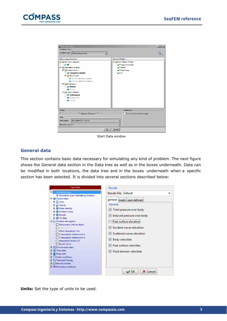
Start Data window

When starting up the Tdyn environment, the start data window will pop up. This window is meant to define the interface so that only those features that are necessary for the case study will be available. This way, the interface will show only those parameters and boundary conditions required, hiding those unnecessary, and therefore making it easier to use and navigate through.

The following figure shows the Tdyn environment and the start data window. In order to use SeaFEM, make sure that Seakeeping analysis option is selected from the Simulation type box.

Within the Analysis domain section of the problem selection data tree you can select either frequency or time domain analysis. When selecting the frequency domain option, the remaining options are automatically set up. On the contrary, if the time domain option is selected, then first or second order diffraction radiation options can be choosen depending on the wave order you want to be used for the analysis. Furthermore, under the environment section of the data tree, you can select whether waves and/or currents are to be used. Finally, under the Type of analysis folder, the following three options are available:

Seakeeping:this option will allow the user to activate body movements on those unrestrained degrees of freedoms.Turning circle: this option is meant to simulate a body following a circular trajectory. Therefore, surge, sway and yaw will be restrained.Towing: this option is meant to simulate a ship following linear trajectory with a certain direction and speed. Therefore, surge, sway and yaw will be restrained.

It is obvious that Turning circle and Towing are not compatible options. On the other hand, any other combination of options are compatible simultaneously.

The Start data window can be accessed and modified at any time through the Data menu:

Data Start data

or through the Data tree.

SeaFEM reference


Start Data window

General data

This section contains basic data necessary for simulating any kind of problem. The next figure shows the General data section in the Data tree as well as in the boxes underneath. Data can be modified in both locations, the data tree and in the boxes underneath when a specific section has been selected. It is divided into several sections described below:

Units: Set the type of units to be used.

SeaFEM reference


Gravity: Set the gravity value, the direction and the units.

Water density: Set the water density and the metric unit.

Problem setup: This section is equivalent to the start data window. Values can be modified though the start data or here.

Results: This section is meant to set what kind of results we want to obtain, and in which format they must be written. Note thta if the frequency domain type of analysis is being used it is only necessary to specify the results file format. The rest of the options listed here are only available when a time domain analysis is undertaken.

Results file: select the format in which the results are to be written. Binary formats are less memory consuming. Binary 1 has to be selected if traditional GID post process is to be used. Binary 2 format (default) is to be used if the newer post process is to be used. Additionally, the native Nemoh file format is available for frequency domain analysis.General: select those values to be written in the result files. The values shown under "general" are those field values over meshes. Then, they might cause the result fields to be quite large memory.Loads: Forces and moments acting over the body under study can be recorded along the simulation. Pressure load refers to those loads obtained by integrating the pressure over the body surfaces. total loads refers to all kind of loads, including pressure loads, hydrostatic restoring loads, and any other external load brought into the simulation.Kinematics: in this section, select the variables to be recorded during the simulation. Movements, velocities and accelerations are referred to the gravity center of the body. Raos stand for Response Amplitude operator.User defined: Here, the user can create time dependent outputs. These outputs might be written analytically and might be dependent on any variable involve in the simulation, such as position, velocity or acceleration of the body, pressure over pressurized free surfaces, etc.

Computational domain generation

In order to generate a good quality computational domain, it is advised to the user to follow these recommendations:

When simulating wave spectra with multiple waves, the absorption area should be at least as long as the maximum wave length. Recommended length is twice the maximum wave length. If monochromatic wave is used along with Sommerfeld radiation condition, the absorption area might be reduced to half the wave length. Computational depth should be no larger than physical depth.

SeaFEM reference


If simulating infinite depth, it is advised to set the computational depth to the maximum wave length. Computational depth might be smaller than physical and/or recommended if the bottom boundary condition is used. Care must be taken since the depth of the body should be small compared to the computational depth when using this option.

SeaFEM reference


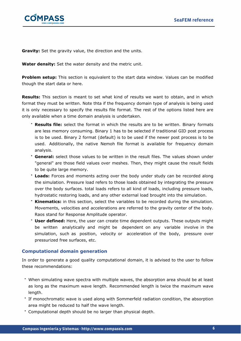
Problem description

In this section, some key parameters necessary to carry out the simulation have to be provided. The following figure shows the data interface. Note that this section of the data tree becomes more simple when using the frequency domain type of analysis. In that case, only the type of bathymetry to be used (and optionally ther corresponding depth) must be specified.

Problem description data interface

Bathymetry

Infinite depth: to be used when the depth is much larger than the wave lengths. In this case, the depth of the domain is recommended to be at least equal to half the wave length of the largest incident wave. However, smaller computational depths can be used in combination with the Bottom boundary condition to simulate lager depths. This can be done when de characteristic length of the body under analysis is small compared to the computational depth. Constant depth: to be used when the bottom is flat, and the depth is constant and smaller than half the wave lengths of the largest wave. Smaller computational depths can be used in combination with the Bottom boundary condition the same way it has been indicated previously.Depth: only available if Bathymetry=Constant depth was selected. The real depth of the problem must be introduced in the box

Wave absorption: select if scattered waves generated by the presence of the body are to be absorbed in order to avoid reflection at the edge of the computational domain. The absorption area will start at a specific distance (Beach)from a reference point located on the free surface. Therefore, there will be no absorption in the circle with center the reference point, and radius the value introduced in "Beach". The area with no dissipation will be referred as the analysis area since no artificial dissipation is introduced on purpose to damp waves refracted and

SeaFEM reference


radiated by the body.

X absorption reference: X coordinate of the reference point to determine the analysis and absorption area.

Y absorption reference: Y coordinate of the reference point to determine the analysis and absorption area.

Absorption factor: determines how strong the dissipation is (recommended value "1”). Large absorption factors might cause instabilities and/or wave reflection. Smaller values, while being less likely to cause instabilities, but will require larger computational domains to damp refracted and radiated waves.

Beach: determine how far, from the reference point, the free surface absorption starts.

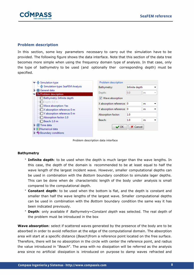
Sommerfeld radiation condition: This option is only available in those cases where the the body is subjected to waves, has no translational movement (turning circle/towing) and is in the absence of currents. In these cases, the largest waves can be hard to be dissipated in the absorption area unless a large computational domain is used. To avoid this situation, a Sommerfeld radiation condition can be used to allow the largest waves to leave the domain across the edge of the computational domain. Therefore, the combined action of the dissipation area and the Sommerfeld radiation condition is the best choice to avoid reflection of waves onto the edges.

Analysis area and wave absorption area

SeaFEM reference


Environment data

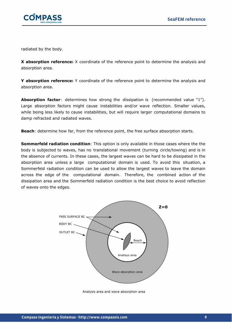
This section is meant to provide the data necessary to simulate the marine environment. Different options are available depending on wether frequency or time domain is under consideration.

Frequency domain:In this case, the wave spectra will be a set of monochromatic waves defined by the period and heading of each wave. The data to be inserted is quite simple and the user only needs to define the following inputs:

- Shortes and Longest Period: Shortest and Longest wave periods that the wave spectra will have.

- Number of waves periods: total number of wave periods to be used in the wave spectra.

- Lower and Upper heading: Lower and Upper wave heading that the wave spectra will have.

- Number of waves headings: Total number of wave headings to be used in the wave spectra.

- Speed: Total forward speed that the bodies will have.

- Speed direction: Direction of the speed for all bodies.

Time domain:Different sort of wave spectra are available for time domain analises, each one requiring of specific data. The wave spectra is introduced in SeaFEM as an incident velocity potential.

SeaFEM reference


Environment data interface

Wave environment data and currents environment data can be defined through the menu options:

Environment data Waves

and

Environment data Currents

respectively.

Wave environment data

Next is a description of the different inputs to be provided by the user:

Wave spectrum type: select the type of incident wave environment. The following options are available.

Monochromatic wave: this is the simplest spectrum available. This option generates an incident wave that corresponds to a monochromatic wave. In order to determine this monochromatic wave, the wave amplitude, period and direction of propagation must be provided.

Wave parameters

SeaFEM reference


Pearson Moskowitz spectrum: S(T)=Hs2Tm(0.11/2π)(Tm/T) - 5exp[ - 0.44(Tm/T) - 4],

where T is the wave period; Hs is the significant wave height; Tm is the mean wave

period, which is obtained via Tm =2πm0/m1, with m0 and m1 the zero and first

moments of the wave spectrum. This is probably the simplest idealized spectrum, obtained by assuming a fully developed sea state, generated by wind blowing steadily for a long time over a large area. For further information, please refer to the SeaFEM Theory Manual. Jonswap2 spectrum: The JONSWAP spectrum was established during a joint research project, the "JOint North Sea WAve Project". This is a peak-enhanced Pierson-Moskowitz spectrum given on the form S(ϖ)=(5/16 · Hs

2 · (T 5/Tp4)/(2π)) · exp( - 1.25(Tp/T) - 4) · (1 - 0.287 · log(γ)) · γY,

Y=exp[ - ((0.159ϖTp - 1)/(σ√2))2], where ω=2π/T, σ=0.07 for ω<=6.28/Tp, σ=0.09 for

ω>6.28/Tm, T is the wave period; Hs is the significant wave height, Tp is the peak wave

period and γ is the peakedness parameter. For further information, please refer to the SeaFEM Theory Manual.Jonswap spectrum: An alternative definition of the JONSWAP spectrum given by S(ϖ)=(155Hs

2/(Tm4 ϖ5)) · exp[ - 944Tm

- 4ϖ - 4](3.3)Y, Y=exp[ - ((0.191ϖTm - 1)/(σ√2))2],

where ω=2π/T, σ=0.07 for ω<=5.24/Tm, σ=0.09 for ω>5.24/Tm, T is the wave period;

Hs is the significant wave height; Tm is the mean wave period, which is obtained via

Tm

=2πm0/m1 , with m0 and m1 the zero and first moments of the wave spectrum. For

further information, please refer to the SeaFEM Theory Manual.White noise: introduce a number of waves with frequencies uniformly distributed across an interval, and with same amplitude and direction. This spectrum is used to carry out response amplitude operator (RAO) analysis.Customize: a spectrum can be defined based on the significant wave height and mean wave period.Read from file: by using this option, any generic wave spectrum can be defined by the user. To this aim, a text file must be provided in the data tree entry that becomes available when rhe 'Read from file' option is selected. In the text file the user must indicate the relevant wave parameters (period T, amplitude A, wave direction G and wave phase P) for each wave component conforming the spectrum. The specific format of the wave spectrum file can be viewed in the following example.

SeaFEM Spectrum_file version 1.0NWaveComponents 20TWaves AWaves GWaves PWaves14.6613 2.56028e-005 -0.349066 2.9405312.6662 0.000229263 -0.116355 3.1478813.7174 0.000229263 0.116355 4.55531

SeaFEM reference


11.8723 2.56028e-005 0.349066 2.255667.21275 0.0123038 -0.349066 2.921687.73874 0.110176 -0.116355 0.9173458.79714 0.110176 0.116355 5.202487.21466 0.0123038 0.349066 3.091335.66508 0.0427017 -0.349066 5.925045.86992 0.382376 -0.116355 2.745756.4778 0.382376 0.116355 3.801335.77667 0.0427017 0.349066 0.9676115.33589 0.0272918 -0.349066 2.406465.20454 0.244386 -0.116355 4.505044.92538 0.244386 0.116355 5.629735.17884 0.0272918 0.349066 4.567884.13839 0.0189668 -0.349066 3.386644.07775 0.16984 -0.116355 5.736554.20474 0.16984 0.116355 1.884964.65867 0.0189668 0.349066 5.62345

This user defined spectrum file is equivalent to a Jonswap spectrum realization with the following characteristics:

-Mean wave period = 5 sec.

-Significant wave height = 2 m.

-Shortest period = 4 sec.

-Longest period = 15 sec.

-Number of wave periods = 5

-Mean wave direction = 0 deg.

-Spreading angle = 40 deg.

-Number of wave directions = 4

Customize spectrum: if the option "customize" has been selected in "Wave spectrum type", the user can introduced a spectrum based on the significant wave height and mean wave period. For instance, a Pearson moskowitz spectrum could be written as follows:

(Hs2 · Tm) ·

0.112 · π

·(ws ·Tm

2 · π ) - 5· e - 0.44 · (ws ·

Tm

2 · π ) - 4

SeaFEM reference


where Hs represents the significant wave height; Tm represents the mean wave period,

ws represent the wave frequency ω=2π/T (See appendix A).

Directional wave energy: this variable allows the introduction of a directional wave nergy distribution f(θ), aiming at reproducing spectra with higher energy around the mean direction of propagation, and decaying as the direction diverge from the mean A typical directional wave energy distribution can be expressed as:

f(θ)=cos2(2θ3 ), where θ=π ·

γ - γmγmax - γmin

and θ goes from -π/2 to π/2. This directional energy distribution should be introduced with the following syntax:

cos2(23

· γs · π)

Directional wave energy examples.

Amplitude: amplitude of monochromatic wave or amplitude for white noise spectrum waves.

Period: period of monochromatic wave.

Heading: direction of monochromatic wave or direction for white noise spectrum waves.

SeaFEM reference


Mean wave period: mean wave period for wave spectrum such as Pearson Moskowitz, Jonswap, etc.

Significant height: significant wave period for wave spectrum such as Pearson Moskowitz, Jonswap, etc.

Shortest period: correspond to the wave with maximum frequency to be considered when discretizing a spectrum. Tmin=Tm/2.2 recommended.

Longest period : correspond to the wave with minimum frequency to be considered when discretizing a spectrum. Tmax=2.2Tm recommended.

Number of wave periods: or number of wave frequencies to be used.

Mean wave heading: mean direction of wave propagation. It is provided in the form of an angle θ measured with respect to the X global axis.

Spreading angle: angular sector Δθ within which the waves propagate. Such an angular sector is always centered at the mean wave heading so that the waves propagate within the range [θ - Δθ/2, θ + Δθ/2]

Number of wave headings: in case the waves propagate within an angular sector specified by the mean wave heading and the spreading angle, this parameter determines how many directions such an angular sector will be discretized into.

Realization repeatibility: this option must be activated if the user wishes to run exactlly the same spectrum realization in further simulations. By contrast, if such an option remains deactivated, random realizations of the same given spectrum will be used when running the simulation several times.

Note: the total number of waves used in the realization will be the "number of wave periods” times ”Number of wave directions”.

SeaFEM reference


Pearson Moskowitz discretization. Hs=1; Tm=1; Tmax=2.2Tm; Tmin=Tm/2.2; N=20.

Currents environment data

Next is a description of the various inputs to be provided by the user when using currents:

Velocity: velocity of the water current.

Direction: direction of the water current.

Time data

In this section, several parameters regarding the timing of the simulation are to be defined. Note that time data presented in this section only concern to time domain analysis but not frequency domain.

SeaFEM reference


Time data interface

Simulation time: length in time of the simulation.

Time step: time step to be use for the time marching schemes. The time step introduced in this box will be the one used unless a zero value is introduced. If a zero value is introduced, the time step will be internally calculated by SeaFEM based on the minimum mesh size and the stability parameter β=g∆t2/∆zmin.

Output step: time lag between recordings. Values corresponding between two time steps are linearly interpolated between the previous and the next time step.

Start time recording: set the point in time when the writing of the results will start.

Initialization time: set an initialization time period. During this period, the wave amplitudes and currents will be increased smoothly from zero to their final values following this expression: Initialization factor = 0.5·(1-cos(π·time/timeinit)). This initialization process is

meant to avoid long transient behaviours due to sudden initializations. Sudden initializations may lead to an unrealistic and highly energetic transient behaviours. In this cases, longer simulations are required so the unrealistic high energy behaviour will dissipate over time.

Numerical data

As well as the time data presented in the previous section of the manualo, numerical data shown herein concerns only time domain analysis.

The Numerical data section of the SeaFEM data tree collects information concerning the numerical algorithms underlying the SeaFEM solver. Most of the computational time required by SeaFEM is spent in solving the linear system of equations resulting from the discretization of the governing equations. Therefore, selecting the correct parameters will enhance having

SeaFEM reference


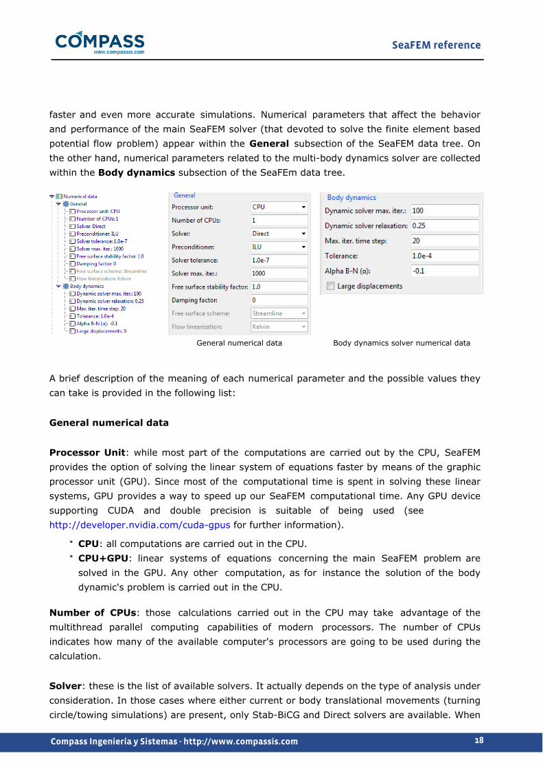
faster and even more accurate simulations. Numerical parameters that affect the behavior and performance of the main SeaFEM solver (that devoted to solve the finite element based potential flow problem) appear within the General subsection of the SeaFEM data tree. On the other hand, numerical parameters related to the multi-body dynamics solver are collected within the Body dynamics subsection of the SeaFEm data tree.

General numerical data Body dynamics solver numerical data

A brief description of the meaning of each numerical parameter and the possible values they can take is provided in the following list:

General numerical data

Processor Unit: while most part of the computations are carried out by the CPU, SeaFEM provides the option of solving the linear system of equations faster by means of the graphic processor unit (GPU). Since most of the computational time is spent in solving these linear systems, GPU provides a way to speed up our SeaFEM computational time. Any GPU device supporting CUDA and double precision is suitable of being used (see http://developer.nvidia.com/cuda-gpus for further information).

CPU: all computations are carried out in the CPU. CPU+GPU: linear systems of equations concerning the main SeaFEM problem are solved in the GPU. Any other computation, as for instance the solution of the body dynamic's problem is carried out in the CPU.

Number of CPUs: those calculations carried out in the CPU may take advantage of the multithread parallel computing capabilities of modern processors. The number of CPUs indicates how many of the available computer's processors are going to be used during the calculation.

Solver: these is the list of available solvers. It actually depends on the type of analysis under consideration. In those cases where either current or body translational movements (turning circle/towing simulations) are present, only Stab-BiCG and Direct solvers are available. When

SeaFEM reference


neither currents nor translational movements exist, the complete list of solvers becomes available. When the CPU+GPU option is being used, the Direct solver is not available in any case.

Conjugate gradient: iterative solver suitable to solve problems leading to a linear set of algebraic equations with a symmetric matrix structureBi-conjugate gradient: iterative solver suitable to solve problems leading to a linear set of algebraic equations with a non-symmetric matrix structureStab bi-conjugate gradient: modified version of the bi-conjugate gradient solver that can provide more stability in some ill-posed numerical problems.Deflated conjugate gradient: deflated version of the conjugate gradient iterative solver. Be aware that the deflation process is not always guaranteed to speed up the solving process. Based on our experience, most of the time it does, but care must be taken when selecting this option. If you feel that SeaFEM is running slow under this option, stop the calculation and select the CG solver instead, compare the speed of the simulation, and act consequently.Direct: direct solver based on the third-party IntelMKL numerical solvers library.

Preconditioner: these is the list of available preconditioners to be used in conjunction with the iterative solvers listed above in order to speed-up the calculations.

if the Processor Unit is set to CPU, the ILU preconditioner is recommended. if the Processor Unit is set to CPU + GPU and neither currents nor translational movements are simulated: the SPAI preconditioner is recommended. if the Processor Unit is set to CPU + GPU and either currents or translational movements are simulated: the Diagonal preconditioner is recommended.

Solver tolerance: maximum tolerance allowed to reach convergence when using iterative solvers. The default value 10-7 is recommended.

Solver max iterations: maximum number of iterations to be carried out by the solver until convergence is achieved. The default value 1000 is recommended.

Free surface stability factor: this factor controls the time step as explained in the time data section, unless a positive time step has been prescribed. If neither currents nor translational movements are simulated, typical values for stability are in the order of 1. If either currents or translational movements are simulated, typical values for stability are in the order of 0.1-0.001, depending on the Froude number. The larger the froude number, the smaller the stability parameter and the time step.

Damping factor: this parameter is available in those cases where the body under study has unrestrained degrees of freedom. Sometimes, the only mechanism to dissipate energy by the body is through wave radiation. However, this mechanism might not be dissipative enough and might cause very long transient periods due to its low dissipation capabilities. This might

SeaFEM reference


be a problem specially when the body is excited with waves whose frequencies are near the resonance frequency of the body. This problem can be mitigated by introducing a small dissipation which is only noticeable near resonance. This is carried out by bringing a percentage of the critical damping into the dynamic equations of the body. It is recommended to use this option only in those cases where it is necessary due to the low wave radiation capacity of the body, and where the body is excited near its resonance frequency. Values between 0 and 0.05 are recommended, depending on the case.

Free surface scheme: this option is only available when either currents or translational movements exist. This parameter actually determines the numerical scheme to be used when solving the free surface boundary condition with convective terms.

Streamlines: in this case, the convective term of the free surface boundary condition is obtained by using a streamline differential operator that actually uses two points upstream and one point downstream to evaluate the derivatives along the streamline.FEM SUPG: this is an alternative method for the integration of the free surface boundary condition. In this case a finite element based SUPG stabilization scheme is used.

Flow linearization: this option is only available when either currents or translational movements exist. It specifies the type of linearization to be used when integrating the convective terms within the free surface boundary condition.

Kelvin: flow around the body is assumed as if is not perturbed by the presence of the body.Double body: flow around the body is assumed as if the free surface behaves as a wall.Non-linear: flow around the body is continously updated to take into account the erpsence of the ody and the effects of waves generated at the free surface.

Body dynamics numerical data

Dynamic solver max. iterations: máximum number of iterations allowed for the dynamic solver.

Dynamic solver relaxation: this parameter concerns the numerical relaxation of the dynamic solver. It must be greater than cero.

Max iterations time step: This parameter is available in those cases where the body under study has unrestrained degrees of freedom. In these cases, an iterative procedure must be carried out within each time step to reach convergence of the body dynamics driven by the hydrodynamic and external loads acting on the body. This parameter sets the maximum number of iterations allowed per time step until convergence is achieved.

SeaFEM reference


Tolerance: maximum tolerance allowed to reach convergence in the iterative procedure carried out within each time step.

Alpha B-N: this parameter concerns the stability of the Bossak-Newmark scheme used to solve the multibody dynamics system. It must take a negative value.

Large displacements: this option must be activated to take into account large displacements when solving the multi-body dynamics system. If this option is active, the inertia matrix of the bodies is updated every time step to take into account the finite rotation of the body. Forces and moments are updated as well to take into account this effect. Note that large displacements have limited application within SeaFEM since the actual position of the body regarding the incident wave is not updated. Hence, caution is adviced when interpreting the results obtained using the large displacements option.

Body data

Body Data section is intended to allow the user to define several bodies and their corresponding properties. The user can create as many bodies as necessary, each one being assigned to a different group of geometrical entities. In the figure below for example, two different bodies have been defined, each one being assigned to a different cylindrical floating body.

Multiple bodies defined through the GUI

For each body, information regarding the mass and the radii's of inertia and unrestrained degrees of freedom must be provided. This is so irrespectively of wether frequency or time

SeaFEM reference


domain options are under consideration. If a time domain calculation is undertaken, additional external forces and moments can be defined for each body.

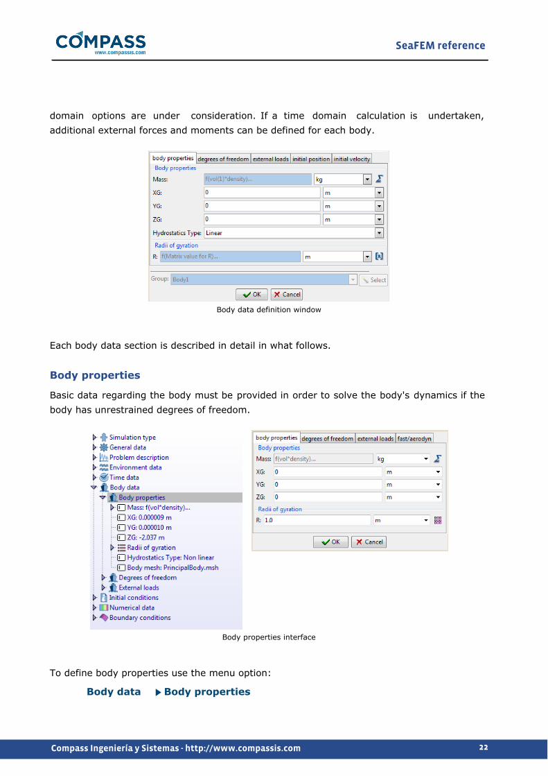
Body data definition window

Each body data section is described in detail in what follows.

Body properties

Basic data regarding the body must be provided in order to solve the body's dynamics if the body has unrestrained degrees of freedom.

Body properties interface

To define body properties use the menu option:

Body data Body properties

SeaFEM reference


Mass: the body mass can be introduced in two different ways: either introducing the exact value or using the function editor. When using the function editor, the mass can be calculated as an analytical value depending of some variables used by SeaFEM. For example, for freely floating objects where the mas must equal the mass of the displaced water, we could write Mass=volume·density, where volume refers to the displaced water volume, and density refers to the water density. This specific case is shown in the following figure.

Mass function editor

XG: introduce the x coordinate of the gravity center of the body.

YG: introduce the y coordinate of the gravity center of the body.

ZG: introduce the z coordinate of the gravity center of the body.

Radii of gyration: the elements of the inertial matrix are related to the radii of gyration as: Iii=Mass·rii·rii; Pij=Mass·rij·|rij|. Then:

rxx: rxx=√Ixx/Mass

rxy: rxy=(Pxy/|Pxy|) · √|Pxy|/Mass

rxz: rxz=(Pxz/|Pxz|) · √|Pxz|/Mass

ryy: ryy=√Iyy/Mass

ryz: ryz=(Pyz/|Pyz|) · √|Pyz|/Mass

rzz: rzz=√Izz/Mass

Radii of gyration matrix interface

SeaFEM reference


Hydrostatic type: this parameter has two possible values, Linear and Non-Linear. By default, the linear option is used so that the calculation of the hydrostatic recovery forces is linearized. By doing this, the displacements of the floating structure are assumed to be small and the hydrostatic restoration coefficients assumed to be constant. This allows for the coefficients to be calculated just once at the beginning of the simulation taking into account the initial configuration. By using the non-linear option, the hydrostatic restoration coefficients are assumed to depend on the actual movement of the floating structure and they must be evaluated at each time step. To this aim, an auxiliary body mesh (containing the entire body) is necessary for tracking the actual position of the body surface during the simulation, thus allowing for the propper integration of the hydrostatic pressure. Such an auxiliary mesh must be generated for each body under analysis and exported in a text file using GiD mesh format. The generated mesh file must be provided as "Body mesh" option under Body properties.

The Non-Linear hydrostatic type option allows for the simulation of those phenomena that are inherently non-linear as for instance the parametric resonance.

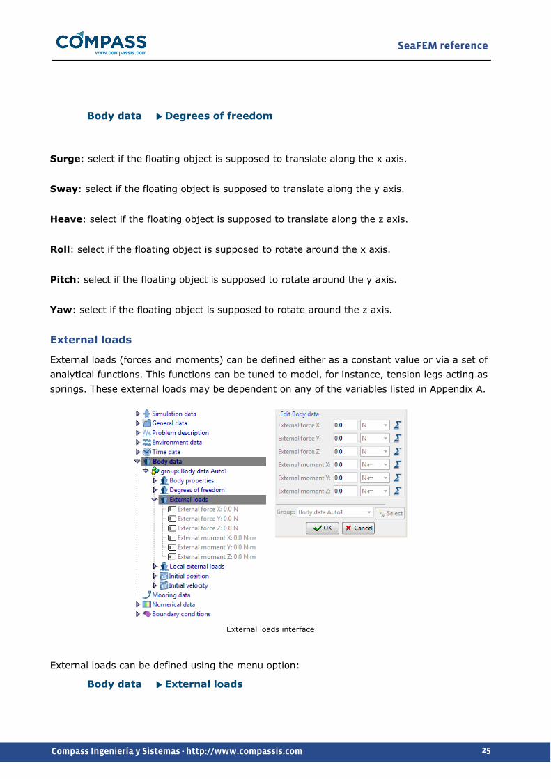
Degrees of freedom

Next figure shows the interface where the user can activate/deactivate the unrestrained degrees of freedom. When performing analysis such as Turning circle or Towing, the Surge,Sway and Yaw are restrained degrees of freedom since the body is forced to follow a specific trajectory, while the Heave, Roll and Pitch are unrestrained.

Degrees of freedom interface

Degrees of freedom can be activated/deactivated through the menu option:

SeaFEM reference


Body data Degrees of freedom

Surge: select if the floating object is supposed to translate along the x axis.

Sway: select if the floating object is supposed to translate along the y axis.

Heave: select if the floating object is supposed to translate along the z axis.

Roll: select if the floating object is supposed to rotate around the x axis.

Pitch: select if the floating object is supposed to rotate around the y axis.

Yaw: select if the floating object is supposed to rotate around the z axis.

External loads

External loads (forces and moments) can be defined either as a constant value or via a set of analytical functions. This functions can be tuned to model, for instance, tension legs acting as springs. These external loads may be dependent on any of the variables listed in Appendix A.

External loads interface

External loads can be defined using the menu option:

Body data External loads

SeaFEM reference


Local external loads

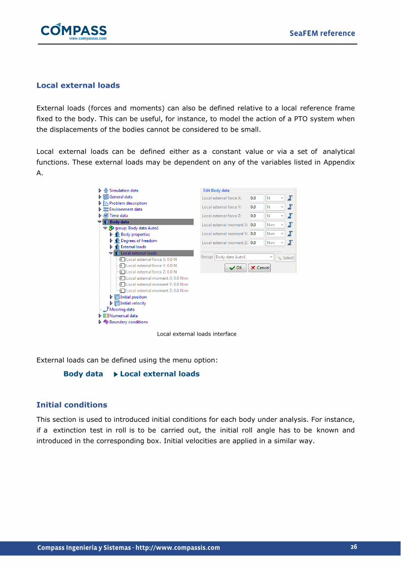
External loads (forces and moments) can also be defined relative to a local reference frame fixed to the body. This can be useful, for instance, to model the action of a PTO system when the displacements of the bodies cannot be considered to be small.

Local external loads can be defined either as a constant value or via a set of analytical functions. These external loads may be dependent on any of the variables listed in Appendix A.

Local external loads interface

External loads can be defined using the menu option:

Body data Local external loads

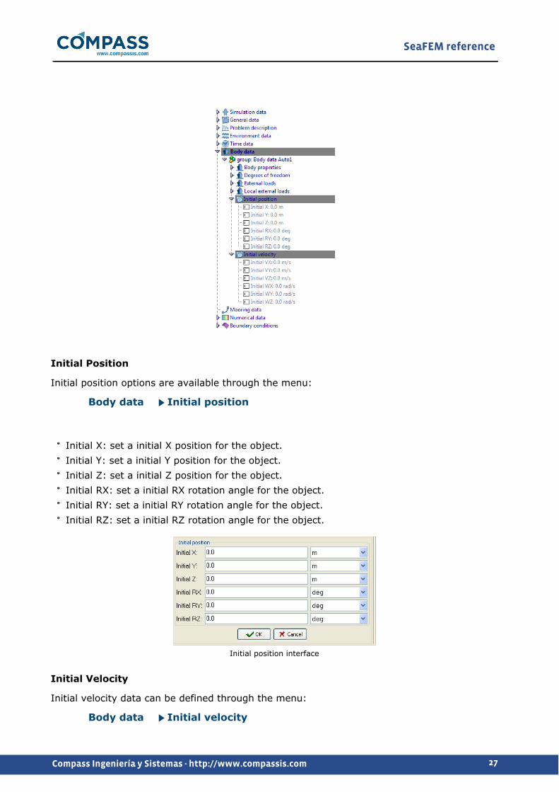
Initial conditions

This section is used to introduced initial conditions for each body under analysis. For instance, if a extinction test in roll is to be carried out, the initial roll angle has to be known and introduced in the corresponding box. Initial velocities are applied in a similar way.

SeaFEM reference


Initial Position

Initial position options are available through the menu:

Body data Initial position

Initial X: set a initial X position for the object.Initial Y: set a initial Y position for the object.Initial Z: set a initial Z position for the object.Initial RX: set a initial RX rotation angle for the object.Initial RY: set a initial RY rotation angle for the object.Initial RZ: set a initial RZ rotation angle for the object.

Initial position interface

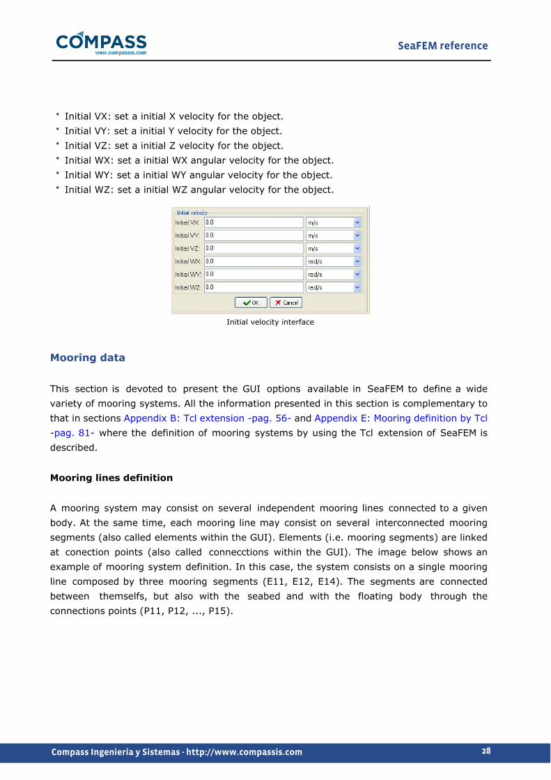
Initial Velocity

Initial velocity data can be defined through the menu:

Body data Initial velocity

SeaFEM reference


Initial VX: set a initial X velocity for the object.Initial VY: set a initial Y velocity for the object.Initial VZ: set a initial Z velocity for the object.Initial WX: set a initial WX angular velocity for the object.Initial WY: set a initial WY angular velocity for the object.Initial WZ: set a initial WZ angular velocity for the object.

Initial velocity interface

Mooring data

This section is devoted to present the GUI options available in SeaFEM to define a wide variety of mooring systems. All the information presented in this section is complementary to that in sections Appendix B: Tcl extension -pag. 56- and Appendix E: Mooring definition by Tcl -pag. 81- where the definition of mooring systems by using the Tcl extension of SeaFEM is described.

Mooring lines definition

A mooring system may consist on several independent mooring lines connected to a given body. At the same time, each mooring line may consist on several interconnected mooring segments (also called elements within the GUI). Elements (i.e. mooring segments) are linked at conection points (also called connecctions within the GUI). The image below shows an example of mooring system definition. In this case, the system consists on a single mooring line composed by three mooring segments (E11, E12, E14). The segments are connected between themselfs, but also with the seabed and with the floating body through the connections points (P11, P12, ..., P15).

SeaFEM reference


New mooring lines can be created by right-clicking over the "Mooring data" option of the data tree and selecting the option "Create a new mooring line". By default, when creating a new mooring line it contains a single element.

Mooring data Create new mooring line

Elements definition

When creating a new mooring line, a single mooring segment is created by default and assigned to the current segment. New mooring segments can be created by copying the previous one and editing the corresponding parameters as they are described in what follows:

Type of mooring : this parameter determines the type of mooring segment to be used. The possible values of this parameter are:

SeaFEM reference


Spring : quasi-static elastic bar (spring able to work in both, tension and compression regimes).Spring only tension : quasi-static cable (spring able to work only in tension)Catenary : quasi-static elastic catenaryDynamic cable : dynamic cable

Length [m] : length of the current mooring element

Area [m2] : cross section area of the element

Young modulus [Pa] : Young modulus of the current mooring element

Effective weight [N/m] : effective weight (actual weight minus bouyancy) per unit length

End A: This field is used to specify the first end point of the current mooring segment. It can be specified by either giving the coordinates of a new point, or by selecting an already existing point of the actual geometry. (See the "Connection definition" section below).

End B: This field is used to specify the second end point of the current mooring segment. It can be specified by either giving the coordinates of a new point, or by selecting an already existing point of the actual geometry. (See the "Connection definition" section below).

Number of elements : this parameter is only enabled when the dynamic FEM cable type of mooring is selected. It determines the number of line elements used in the cable discretization.

Damping a, b : user defined damping ratios for dynamic cables

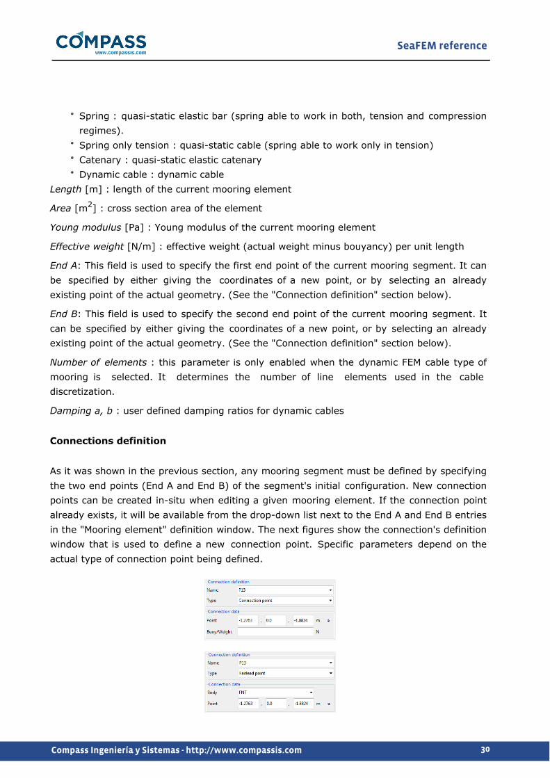
Connections definition

As it was shown in the previous section, any mooring segment must be defined by specifying the two end points (End A and End B) of the segment's initial configuration. New connection points can be created in-situ when editing a given mooring element. If the connection point already exists, it will be available from the drop-down list next to the End A and End B entries in the "Mooring element" definition window. The next figures show the connection's definition window that is used to define a new connection point. Specific parameters depend on the actual type of connection point being defined.

SeaFEM reference


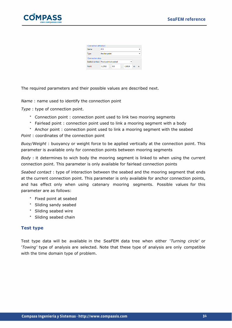
The required parameters and their possible values are described next.

Name : name used to identify the connection point

Type : type of connection point.

Connection point : connection point used to link two mooring segments Fairlead point : connection point used to link a mooring segment with a body Anchor point : connection point used to link a mooring segment with the seabed

Point : coordinates of the connection point

Buoy/Weight : buoyancy or weight force to be applied vertically at the connection point. This parameter is available only for connection points between mooring segments

Body : it determines to wich body the mooring segment is linked to when using the current connection point. This parameter is only available for fairlead connection points

Seabed contact : type of interaction between the seabed and the mooring segment that ends at the current connection point. This parameter is only available for anchor connection points, and has effect only when using catenary mooring segments. Possible values for this parameter are as follows:

Fixed point at seabed Sliding sandy seabed Sliding seabed wire Sliding seabed chain

Test type

Test type data will be available in the SeaFEM data tree when either 'Turning circle' or 'Towing' type of analysis are selected. Note that these type of analysis are only compatible with the time domain type of problem.

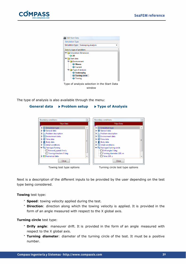
SeaFEM reference


Type of analysis selection in the Start Data window

The type of analysis is also available through the menu:

General data Problem setup Type of Analysis

Towing test type options Turning circle test type options

Next is a description of the different inputs to be provided by the user depending on the test type being considered.

Towing test type:

Speed: towing velocity applied during the test.Direction: direction along which the towing velocity is applied. It is provided in the form of an angle measured with respect to the X global axis.

Turning circle test type:

Drify angle: maneuver drift. It is provided in the form of an angle measured with respect to the X global axis.Turning diameter: diameter of the turning circle of the test. It must be a positive number.

SeaFEM reference


Time: time used to complete the maneuver.

SeaFEM reference


Boundary conditions

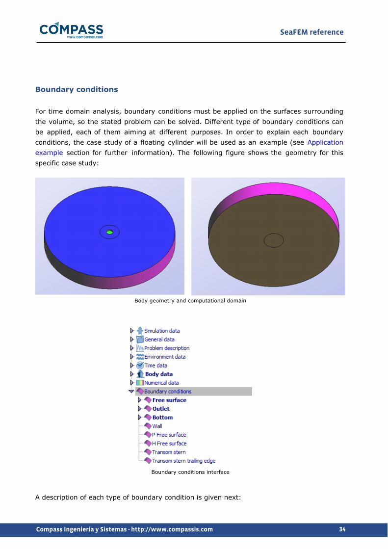
For time domain analysis, boundary conditions must be applied on the surfaces surrounding the volume, so the stated problem can be solved. Different type of boundary conditions can be applied, each of them aiming at different purposes. In order to explain each boundary conditions, the case study of a floating cylinder will be used as an example (see Application example section for further information). The following figure shows the geometry for this specific case study:

Body geometry and computational domain

Boundary conditions interface

A description of each type of boundary condition is given next:

SeaFEM reference


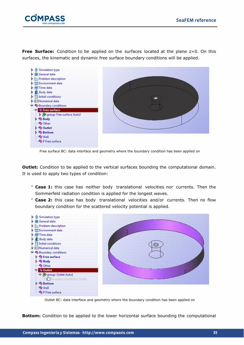
Free Surface: Condition to be applied on the surfaces located at the plane z=0. On this surfaces, the kinematic and dynamic free surface boundary conditions will be applied.

Free surface BC: data interface and geometry where the boundary condition has been applied on

Outlet: Condition to be applied to the vertical surfaces bounding the computational domain. It is used to apply two types of condition:

Case 1: this case has neither body translational velocities nor currents. Then the Sommerfeld radiation condition is applied for the longest waves.Case 2: this case has body translational velocities and/or currents. Then no flow boundary condition for the scattered velocity potential is applied.

Outlet BC: data interface and geometry where the boundary condition has been applied on

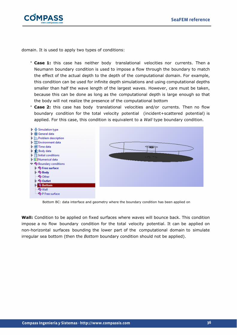
Bottom: Condition to be applied to the lower horizontal surface bounding the computational

SeaFEM reference


domain. It is used to apply two types of conditions:

Case 1: this case has neither body translational velocities nor currents. Then a Neumann boundary condition is used to impose a flow through the boundary to match the effect of the actual depth to the depth of the computational domain. For example, this condition can be used for infinite depth simulations and using computational depths smaller than half the wave length of the largest waves. However, care must be taken, because this can be done as long as the computational depth is large enough so that the body will not realize the presence of the computational bottom Case 2: this case has body translational velocities and/or currents. Then no flow boundary condition for the total velocity potential (incident+scattered potential) is applied. For this case, this condition is equivalent to a Wall type boundary condition.

Bottom BC: data interface and geometry where the boundary condition has been applied on

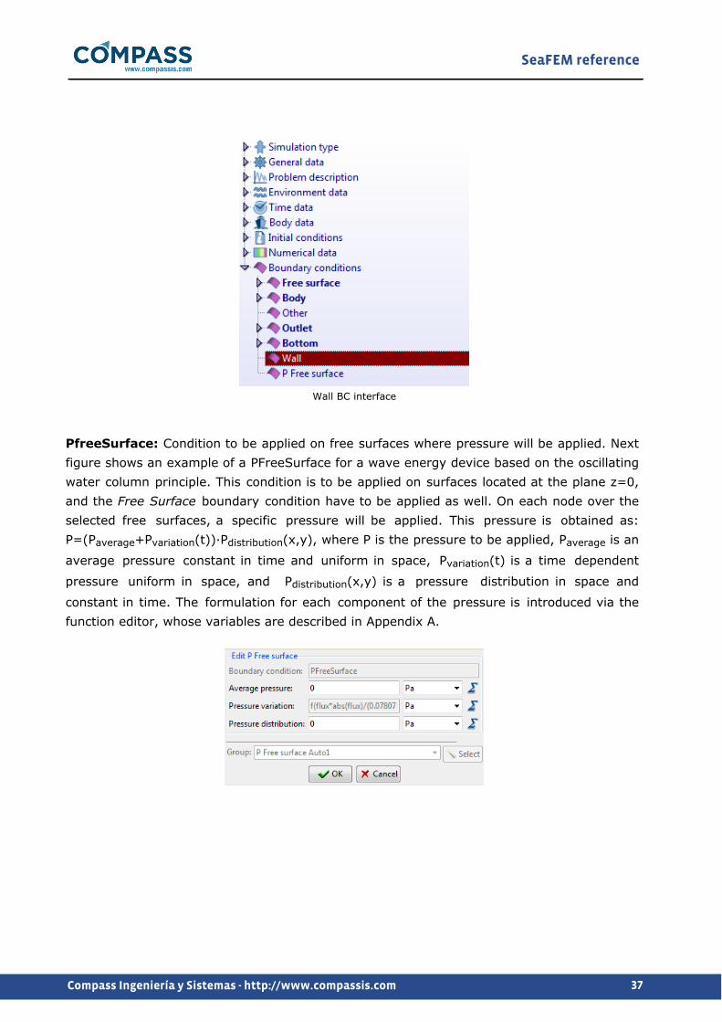
Wall: Condition to be applied on fixed surfaces where waves will bounce back. This condition impose a no flow boundary condition for the total velocity potential. It can be applied on non-horizontal surfaces bounding the lower part of the computational domain to simulate irregular sea bottom (then the Bottom boundary condition should not be applied).

SeaFEM reference


Wall BC interface

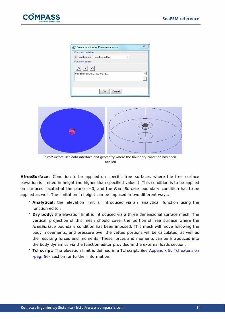
PfreeSurface: Condition to be applied on free surfaces where pressure will be applied. Next figure shows an example of a PFreeSurface for a wave energy device based on the oscillating water column principle. This condition is to be applied on surfaces located at the plane z=0, and the Free Surface boundary condition have to be applied as well. On each node over the selected free surfaces, a specific pressure will be applied. This pressure is obtained as: P=(Paverage+Pvariation(t))·Pdistribution(x,y), where P is the pressure to be applied, Paverage is an

average pressure constant in time and uniform in space, Pvariation(t) is a time dependent

pressure uniform in space, and Pdistribution(x,y) is a pressure distribution in space and

constant in time. The formulation for each component of the pressure is introduced via the function editor, whose variables are described in Appendix A.

SeaFEM reference


PFreeSurface BC: data interface and geometry where the boundary condition has been applied

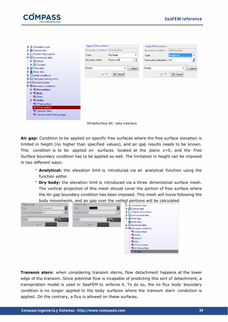
HfreeSurface: Condition to be applied on specific free surfaces where the free surface elevation is limited in height (no higher than specified values). This condition is to be applied on surfaces located at the plane z=0, and the Free Surface boundary condition has to be applied as well. The limitation in height can be imposed in two different ways:

Analytical: the elevation limit is introduced via an analytical function using the function editor.Dry body: the elevation limit is introduced via a three dimensional surface mesh. The vertical projection of this mesh should cover the portion of free surface where the HreeSurface boundary condition has been imposed. This mesh will move following the body movements, and pressure over the vetted portions will be calculated, as well as the resulting forces and moments. These forces and moments can be introduced into the body dynamics via the function editor provided in the external loads section. Tcl script: The elevation limit is defined in a Tcl script. See Appendix B: Tcl extension -pag. 56- section for further information.

SeaFEM reference


HFreeSurface BC: data interface

Air gap: Condition to be applied on specific free surfaces where the free surface elevation is limited in height (no higher than specified values), and air gap results needs to be known. This condition is to be applied on surfaces located at the plane z=0, and the Free Surface boundary condition has to be applied as well. The limitation in height can be imposed in two different ways:

Analytical: the elevation limit is introduced via an analytical function using the function editor.Dry body: the elevation limit is introduced via a three dimensional surface mesh. The vertical projection of this mesh should cover the portion of free surface where the Air gap boundary condition has been imposed. This mesh will move following the body movements, and air gap over the vetted portions will be calculated.

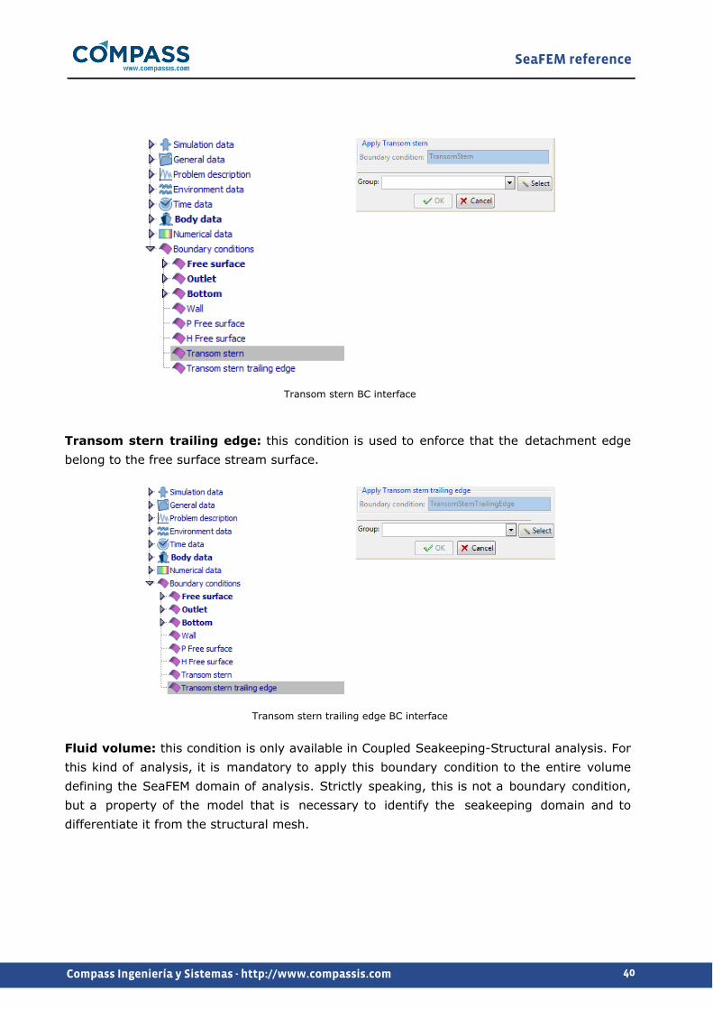
Transom stern: when considering transom sterns, flow detachment happens at the lower edge of the transom. Since potential flow is incapable of predicting this sort of detachment, a transpiration model is used in SeaFEM to enforce it. To do so, the no flux body boundary condition is no longer applied to the body surfaces where the transom stern condiction is applied. On the contrary, a flux is allowed on these surfaces.

SeaFEM reference


Transom stern BC interface

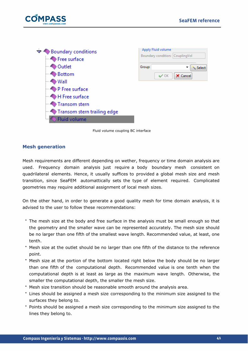
Transom stern trailing edge: this condition is used to enforce that the detachment edge belong to the free surface stream surface.

Transom stern trailing edge BC interface

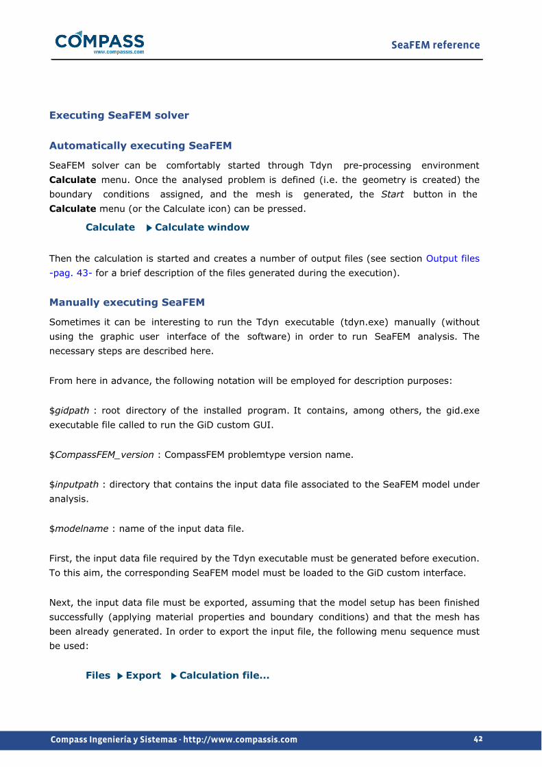
Fluid volume: this condition is only available in Coupled Seakeeping-Structural analysis. For this kind of analysis, it is mandatory to apply this boundary condition to the entire volume defining the SeaFEM domain of analysis. Strictly speaking, this is not a boundary condition, but a property of the model that is necessary to identify the seakeeping domain and to differentiate it from the structural mesh.

SeaFEM reference


Fluid volume coupling BC interface

Mesh generation

Mesh requirements are different depending on wether, frequency or time domain analysis are used. Frequency domain analysis just require a body boundary mesh consistent on quadrilateral elements. Hence, it usually suffices to provided a global mesh size and mesh transition, since SeaFEM automattically sets the type of element required. Complicated geometries may require additional assignment of local mesh sizes.

On the other hand, in order to generate a good quality mesh for time domain analysis, it is advised to the user to follow these recommendations:

The mesh size at the body and free surface in the analysis must be small enough so that the geometry and the smaller wave can be represented accurately. The mesh size should be no larger than one fifth of the smallest wave length. Recommended value, at least, one tenth. Mesh size at the outlet should be no larger than one fifth of the distance to the reference point. Mesh size at the portion of the bottom located right below the body should be no larger than one fifth of the computational depth. Recommended value is one tenth when the computational depth is at least as large as the maximum wave length. Otherwise, the smaller the computational depth, the smaller the mesh size. Mesh size transition should be reasonable smooth around the analysis area. Lines should be assigned a mesh size corresponding to the minimum size assigned to the surfaces they belong to. Points should be assigned a mesh size corresponding to the minimum size assigned to the lines they belong to.

SeaFEM reference


Executing SeaFEM solver

Automatically executing SeaFEM

SeaFEM solver can be comfortably started through Tdyn pre-processing environment Calculate menu. Once the analysed problem is defined (i.e. the geometry is created) the boundary conditions assigned, and the mesh is generated, the Start button in the Calculate menu (or the Calculate icon) can be pressed.

Calculate Calculate window

Then the calculation is started and creates a number of output files (see section Output files -pag. 43- for a brief description of the files generated during the execution).

Manually executing SeaFEM

Sometimes it can be interesting to run the Tdyn executable (tdyn.exe) manually (without using the graphic user interface of the software) in order to run SeaFEM analysis. The necessary steps are described here.

From here in advance, the following notation will be employed for description purposes:

$gidpath : root directory of the installed program. It contains, among others, the gid.exe executable file called to run the GiD custom GUI.

$CompassFEM_version : CompassFEM problemtype version name.

$inputpath : directory that contains the input data file associated to the SeaFEM model under analysis.

$modelname : name of the input data file.

First, the input data file required by the Tdyn executable must be generated before execution. To this aim, the corresponding SeaFEM model must be loaded to the GiD custom interface.

Next, the input data file must be exported, assuming that the model setup has been finished successfully (applying material properties and boundary conditions) and that the mesh has been already generated. In order to export the input file, the following menu sequence must be used:

Files Export Calculation file...

SeaFEM reference


By doing this, the user will be asked for a file name ($modelname) and location ($inputpath). By default, .dat extension will be used to export de input file. If desired, .flavia extension can be also specified for instance, trying to mimic the file name convention used when running SeaFEM solver automatically.

Before execution, you must ensure that the tdyn.exe process is able to find a password.txt file containg a valid tdyn password. You can create such a text file manually and copying the password inside. Alternatively, the password.txt file can be copied from the directory $gidpath\problemtypes\$CompassFEM_version\compassfem.gid , where it is automatically saved if tdyn passwords have been previously registered through the GiD custom GUI. For manual execution of the solver, the password file must be located either next to the tdyn.exe executable (this is on the previously mentioned $gidpath\problemtypes\$CompassFEM_version\compassfem.gid\exec directory) or next to the input file.

After exporting the input file and copying a valid password.txt file, everything is ready to launch tdyn.exe manually. To this aim, open a command shell and move to the location of the tdyn.exe executable. Such a location will be typically of the form:

$gidpath\problemtypes\$CompassFEM_version\compassfem.gid\exec

Note that tdyn.exe may be also executed from an arbitrary location if the directory path above is convinientlly added to the environment system variable PATH.

Finally, launch tdyn by using the following command line:

\:> tdyn.exe -name "$inputpath\$modelname" -SeaWaves

Output files generated during process execution

The output files described in the following section concern to the global analysis.

ProblemName.flavia.inf : Text file containing global information as well as process information for each time step. The content of this file can also be accessed during calculation through the GUI by using the menu option Calculate > View process info.

ProblemName.flavia.out : Text file containing iterations and convergence history.

ProblemName.flavia.tim : XML file that contains a timetable in XML format giving information on the CPU time consumption of the process. The timetable contains a report of the execution time used by different parts of the problem. This file is only available after complete successful calculation of a problem.

SeaFEM reference


ProblemName.flavia.err : Text file containing error messages (file created only if tdyn.exe exits with an error).

ProblemName.flavia.res : Main results file that contains all field valued results. When pressing Postprocess in Custom GiD, this file is loaded, and the results it contains can be visualized in the post-processing module. Also note that each calculation will delete a previous results file that might exist in this directory, unless it has been renamed before the new calculation process has been started.

ProblemName.flavia.ram.msh : Mesh for structural analysis using Ram-Series.

The output files described in the following section concern to the results of the mooring system.

MooringResults.msh : Mesh file containing the nodes coordinates of the mooring segments mesh for the initial configuration. For post-process animation, the coordinates of the initial mesh are updated according to the displacement results saved in MooringResults.res during calculation.

ProblemName.MooringData.res : Text file containing time evolution data of the tension force on both ends of each mooring segment.

MooringResults.res : Text file that contains displacement results (componets and module) at mooring mesh nodes. This results are necessary for animation of the mooring lines in the postprocess.

The output files described in the following section concern to time evolution results on bodies.

Results contained in these files can be visualized using the SeaFEM graphs utility in the SeaFEM postprocessor (see for instance section Results visualization).

ProblemName.BodyKinematics.res : Text file containing time history data of body movements, velocities and accelerations of all bodies under analysis. The complete set of data (all those kinematic results selected for output in the data tree) is written first for the first body defined in the GUI. The rest of bodies data results are written following the order the bodies are defined in the GUI.

ProblemName.BodyLoads.res : Text file containing time history data of body loads and moments acting over all bodies under analysis. The complete set of data (all those kinematic results selected for output in the data tree) is written first for the first body defined in the

SeaFEM reference


GUI. The rest of bodies data results are written following the order the bodies are defined in the GUI. Different components of forces and moments are written separately. Hence, total forces, reactions, hydrostatic pressure forces and dynamic pressure forces can be assessed separately.

ProblemName.Outputs.res : Text file containing time evolution data of the user defined results. (Up to 10 custom results can be defined by the user in the User defined data tree entry).

MooringLoads.res : Text file containing time evolution data of the mooring loads acting on bodies.

The output files described in the following section concern the body animation results.

Results contained in these files can be used to setup body animations within the postprocessor (see for instance section Results visualization).

ProblemName.BodyMovements_animations.res : Text file containing time history data of the movements of the first body defined in the GUI of SeaFEM (refered to the global frame of reference located at the origin 0,0,0).

BodyMovements_animations_#.res : # stands for an integer index that identifies the body to which the file under consideration refers. These are text files similar to the previous one and concerning the remaining bodies defined in the analysis.

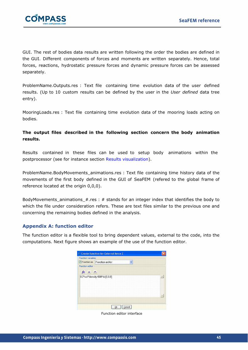
Appendix A: function editor

The function editor is a flexible tool to bring dependent values, external to the code, into the computations. Next figure shows an example of the use of the function editor.

Function editor interface

SeaFEM reference


The following operators can be used in the definition of functions:

Basic operators:

+ : adding operator.Syntax: [adding_expression] + [adding_expression].- : substraction operator.Syntax: [substraction_expression] - [substraction_expression].^ : exponent operator.Syntax: [exponent_expression] ^ [function_expression].* : multiplicative operator.Syntax: [multiplicative_expression] * [multiplicative _expression]./ : division operator.Syntax: [multiplicative_expression] / [quotient_expression].div : integer division operator int(x/y+0.5).Syntax: ([multiplicative_expression]) div ([quotient_expres-sion]). Example: (x)div(2+y).idiv : integer division operator int(x/y+0.5). Similar to div operator but with different syntax.Syntax: idiv ([multiplicative_expression], [quotient_expres-sion]). Example: idiv(x,2+y).mod : integer division module operator int(x+0.5)%int(y+0.5).Syntax: ([multiplicative_expression]) mod ([quotient_expres-sion]). Example: (t)mod(2).imod : integer division module operator int(x+0.5)%int(y+0.5). Similar to mod operator but with different syntax.Syntax: imod ([multiplicative_expression],[quotient_expres-sion]). Example: imod(t,2).rdiv : real division operator int(x/y).Syntax: ([multiplicative_expression]) rdiv ([quotient_expres-sion]). Example: (t)rdiv(5).ddiv : real division operator int(x/y). Similar to rdiv operator but with different syntax.Syntax: ddiv ([multiplicative_expression], [quotient_expres-sion]). Example: ddiv(t,5).rmod : real division module operator x/y-int(x/y).Syntax: ([multiplicative_expression]) rmod ([quotient_expres-sion]). Example: (t)rmod(5).dmod : real division module operator x/y-int(x/y). Similar to rmod operator but with different syntax.Syntax: dmod ([multiplicative_expression], [quotient_expres-sion]). Example: dmod(t,5).max : maximum operator.Syntax: max ([expression], [expression]). Example: max(x,y).min : minimum operator.Syntax: min ([expression], [expression]). Example: min(x,y).not : not operator.Syntax: not([function_expression]).~ : not operator.

SeaFEM reference


Syntax: ~([function_expression]).

Examples:

(2*dy)

(5*(dy+1))/2

(dz*dy)mod(5)

imod(dz*dy) (5)

(5^4)

Relational operators:

The relational (binary) operators compare their first operand with their second operand to test validity of the specified relationship. The result of the relational expression is 1 if the tested relationship is true and 0 if it is false. The binary operators that can be used for functions definitions are:

< : less than operator.Syntax: [expression] < [expression].< = : less or equal than operator.Syntax: [expression] <= [expression].>= : greater or equal than operator.Syntax: [expression] >= [expression].> : greater than operator.Syntax: [expression] > [expression].= : equal operator.Syntax: [expression] = [expression].~= : not equal operator.Syntax: [expression] != [expression].& : and operator.Syntax: [expression] & [expression].| : and operator.Syntax: [expression] | [expression].

Examples:

(dy>2)

(dx<=1)

(dx!=1)

(dy>2)&(dx>2)&(dx<3)&(dy<3)

if-else statement:

SeaFEM reference


The if statement controls conditional branching. The body of the if statement (elif_expression) is executed if the value of the expression is non zero. The syntax for the if statement is the following:

if(expression)then(elif_expression)else(next_expression)endif

being elif_expression an additional expression that may include an elif clause with next form:

(expression2)elif(elif_expression2)then(next_expression2)

Examples:

if(dy>2)then(if(x<1)then(1)else(0)endif)else(0)endif

if(dy>2)then(1)elif(dx<1)then(2)else(0)endif

Function operators:

The function operators calculate the value of a standard function at the point defined by the given argument. The function operators that can be used for the definition of the functions are:

sqrt : the sqrt function calculates the square root of the argument. Syntax: sqrt(.)abs : the abs function calculates the absolute value of the argument. Syntax: abs(.)ln : logarithm of the argument, e base. Syntax: ln(.)log : logarithm of the argument, decimal base. Syntax: log(.)fac : factorial of the argument. Syntax: fac(.)sin : sine of the argument. Syntax: sin(.) (argument given in radians).cos : cosine of the argument. Syntax: cos(.) (argument given in radians).tan : tangent of the argument. Syntax: tan(.) (argument given in radians).asin : The asin function returns the arcsine of the argument in the range -π/2 to π/2 radians. Syntax: asin(.).acos : The acos function returns the arccosine of the argument in the range 0 to À radians. Syntax: acos(.).atan : The atan function returns the arctangent of the argument in the range -π/2 to π/2 radians. Syntax: atan(.) (result given in radians).sinh : hyperbolic sine of the argument. Syntax: sinh(.).cosh : hyperbolic cosine of the argument. Syntax: cosh(.).tanh : hyperbolic tangent of the argument. Syntax: tanh(.).exp : the exp function calculates the exponential value of the argument. Syntax: exp(.).heaviside : the heaviside function evaluates Hs defined as:

Hε(Φ)=0 Φ<-ε

Hε(Φ)=1/2 (1+Φ/ε+1/π sin(π*Φ/ε)) |Φ|<ε

SeaFEM reference


Hε(Φ)=1 Φ>ε

The syntax of the function is heaviside(.,.), where the first argument is Φ and the second ε.

Interpolate : performs a linear interpolation, based on the given data. Two arguments are required: a list of pairs (ξ,η), defining a polylineal curve, and a function defining the point (ξ) where the evaluation is to be done. Syntax: interpolate(#ξ1,η1,ξ2,η2,ξ3,η3,...#.).

InterpolateSpline : performs a spline interpolation, based on the given data. Two arguments are required: a list of pairs (ξ,η), defining a the curve, and a function defining the the point (ξ) where the evaluation is to be done. Syntax: interpolatespline(#ξ

1,η

1,ξ

2,η2,ξ3,η3,...#.).

InterpolateFile : performs a spline interpolation, based on the data given in a file. Two arguments are required: a file name where a list of pairs (ξ,η), defining a the curve, is given, and a function defining the the point (ξ) where the evaluation is to be done. Syntax: Interpolatefile(., .), where the first argument in the filename, and the second a function defining the value.srand : The rand function returns a pseudorandom integer in the range 0 to 1, based on the argument given as seed. Syntax: srand(.).int : Integer conversos. Syntax: int(.).- : change sign operator. Syntax: (-expression).j0 : Calculates Bessel function of first kind and order 0, at the given point. Syntax: j0(.).j1 : Calculates Bessel function of first kind and order 1, at the given point. Syntax: j1(.).jn : Calculates Bessel function of first kind and order n, at the given point. Syntax: jn(.,.), where the first argument is the evaluation point and the second is the order of the Bessel function.y0 : Calculates Bessel function of second kind and order 0, at the given point. Syntax: y0(.).y1 : Calculates Bessel function of second kind and order 1, at the given point. Syntax: y1(.).yn : Calculates Bessel function of second kind and order n, at the given point. Syntax: yn(.,.), where the first argument is the evaluation point and the second is the order of the Bessel function.Readfile : Execute the function in the ASCII file defined by the argument. The file must include a first line defining the maximum time to use the function and a second line containing the function to be executed. If the current time is greater than the one defined in the file, the execution is paused until the file is updated.

Syntax readfile(.) where the argument is the path and name of the file. Example readfile(C:\Temp\velx.dat). Example of file format:

Time = 0.1;

Function = "interpolate(#0.0,1.1,1.0,2.0#t);";

Tcl : Executes a TCL script or procedure returning a double value.

SeaFEM reference


Syntax tcl(.) where the argument is the script to be executed. Example tcl(set var) return the value of tcl variable var.

Note: In order to use this function, TCL extension must be enabled by activating Tcl extension.

CloudOfDataFile : performs a local interpolation based on the cloud of points (x,y,z) and data (¸) given in a file. The argument is the path and name of the text file. Syntax: CloudOfDataFile(·), where the argument in the filename. Example CloudOfDataFile(C:\Temp\velx.dat). Example of file format:

0.0 0.0 0.0 1.0

0.0 1.0 0.0 0.5

1.0 1.0 1.0 2.0

5.0 2.5 2.0 5.0

Examples:

2*sqrt(dy)

dx*fac(5)

srand(0)

log(abs(dx))

exp(5)

interpolate(#1.0,2.0,2.0,2.5,3.0,2.0#t^2)

Specific variables:

Furthermore, the following variables can be used in the definition of functions. Note that some of these variables refer to the main body (index 1). In order to access the corresponding variable for other bodies, the index of the body must be given in parentheses ( examples: dx(2)[0,0,0], vx(3) ).

GENERAL VARIABLES

time or t : Process time (unit: s). gravity or g : Magnitud of gravity (unit: m/s2). density : Fluid density (unit; kg/m·s2). ts or dt : time increment (unit: s). Init_factor : returns the current initialization factor (if the initialization time option is used)

WAVE SPECTRUM VARIABLES

SeaFEM reference


Hs : Significant wave height (unit: m). Tm : Mean wave period (unit: s). W_s : Wave frequency (unit: s-1) Gamma_s : Wave direction (unit: º).

FREE SURFACE VARIABLES

eta : Free surface elevation at the specified node eta_prev : Free surface elevation at the specified node (previous step)

BODY's VARIABLES

vol or volume : Water volume displaced by body (unit: m3). disp : Mass of water displaced by body (unit: kg). Wet_surface : Area of body surface under still water level (unit: m2). xc : X coordinate of the body buoyancy center (unit: m). yc : Y coordinate of the body buoyancy center (unit: m). zc : Z coordinate of the body buoyancy center (unit: m). xg : X coordinate of the body gravity center (unit: m). yg : Y coordinate of the body gravity center (unit: m). zg : Z coordinate of the body gravity center (unit: m). k11 : Surge hydrostatic restoring coeficient. (unit: N/m). k22 : Sway hydrostatic restoring coeficient. (unit: N/m). k33 : Heave hydrostatic restring coeficient. (unit: N/m). k44 : Roll hydrostatic restoring coeficient. (unit: N/rad). k55 : Pitch hydrostatic restoring coeficient. (unit: N/rad). k66 : Yaw hydrostatic restoring coeficient. (unit: N/rad). mass : Body mass. (unit: kg). Ixx : Inertial moment respect to X direction and gravity center (unit: Kg·m2). Iyy : Inertial moment respect to Y direction and gravity center. (unit: Kg·m2). Izz : Inertial moment respect to Z direction and gravity center. (unit: Kg·m2). dx : Translation, in the x direction, of the main body gravity center. (unit: m). dy : Translation, in the y direction, of the main body gravity center. (unit: m). dz : Translation, in the z direction, of the main body gravity center. (unit: m). dx(bodyIdx,stepIdx) : Returns the translation along the x direction of the body given by bodyIdx at a previous time step given by stepIdx. (unit: m). dy(bodyIdx,stepIdx) : Returns the translation along the y direction of the body given by bodyIdx at a previous time step given by stepIdx. (unit: m). dz(bodyIdx,stepIdx) : Returns the translation along the z direction of the body given by bodyIdx at a previous time step given by stepIdx. (unit: m). dx[xi ,yi ,zi]: Translation, in the x direction, of an arbitrary point with coordinates [xi ,yi ,zi] respect to the gravity center. (unit: m). dy[xi ,yi ,zi]: Translation, in the y direction, of an arbitrary point with coordinates [xi ,yi

SeaFEM reference


,zi] respect to the gravity center. (unit: m). dz[xi ,yi ,zi]: Translation, in the z direction, of an arbitrary point with coordinates [xi ,yi ,zi] respect to the gravity center. (unit: m). ldsx : Translation, in the x direction in the local frame. (unit: m). ldsy : Translation, in the y direction in the local frame. (unit: m). ldsz : Translation, in the z direction in the local frame. (unit: m). rx : Rotation, around the x direction, of the body gravity center. (unit: rad). ry : Rotation, around the y direction, of the body gravity center. (unit: rad). rz : Rotation, around the z direction, of the body gravity center. (unit: rad). rx(body,stepIdx) : Returns the rotation around the x direction of the body given by bodyIdx at a previous time step given by stepIdx. (unit: rad). ry(body,stepIdx) : Returns the rotation around the y direction of the body given by bodyIdx at a previous time step given by stepIdx. (unit: rad). rz(body,stepIdx) : Returns the rotation around the z direction of the body given by bodyIdx at a previous time step given by stepIdx. (unit: rad). lrx : Rotation, around the x direction in the local frame. (unit: rad). lry : Rotation, around the y direction in the local frame. (unit: rad). lrz : Rotation, around the z direction in the local frame. (unit: rad). vx : Body velocity in the x direction. (unit: m/s). vy : Body velocity in the y direction. (unit: m/s). vz : Body velocity in the z direction. (unit: m/s). vx(body,stepIdx) : Returns the velocity in the x direction of the body given by bodyIdx at a previous time step given by stepIdx. (unit: m/s). vy(body,stepIdx) : Returns the velocity in the y direction of the body given by bodyIdx at a previous time step given by stepIdx. (unit: m/s). vz(body,stepIdx) : Returns the velocity in the z direction of the body given by bodyIdx at a previous time step given by stepIdx. (unit: m/s). wx: Body angular velocity around the x direction. (unit: rad/s). wy: Body angular velocity around the y direction. (unit: rad/s). wz: Body angular velocity around the z direction. (unit: rad/s). wx(body,stepIdx) : Returns the angular velocity around the x direction of the body given by bodyIdx at a previous time step given by stepIdx. (unit: rad/s). wy(body,stepIdx) : Returns the angular velocity around the y direction of the body given by bodyIdx at a previous time step given by stepIdx. (unit: rad/s). wz(body,stepIdx) : Returns the angular velocity around the z direction of the body given by bodyIdx at a previous time step given by stepIdx. (unit: rad/s). lvx : Body velocity in the x direction in the local frame. (unit: m/s). lvy : Body velocity in the y direction in the local frame. (unit: m/s). lvz : Body velocity in the z direction in the local frame. (unit: m/s). lwx : Body angular velocity around the x direction in the local frame. (unit: rad/s). lwy : Body angular velocity around the y direction in the local frame. (unit: rad/s). lwz : Body angular velocity around the z direction in the local frame. (unit: rad/s).

SeaFEM reference


ax : Body acceleration in the x direction. (unit: m/s2). ay : Body acceleration in the y direction. (unit: m/s2). az : Body acceleration in the z direction. (unit: m/s2). ax(bodyIdx,stepIdx) : Returns the acceleration in the x direction of the body given by bodyIdx at a previous time step given by stepIdx. (unit: m/s2). ay(bodyIdx,stepIdx) : Returns the acceleration in the y direction of the body given by bodyIdx at a previous time step given by stepIdx. (unit: m/s2). az(bodyIdx,stepIdx) : Returns the acceleration in the z direction of the body given by bodyIdx at a previous time step given by stepIdx. (unit: m/s2). lax : Body acceleration in the x direction in the local frame. (unit: m/s2). lay : Body acceleration in the y direction in the local frame. (unit: m/s2). laz : Body acceleration in the z direction in the local frame. (unit: m/s2). arx : Body angular acceleration around the x direction. (unit: rad/s2). ary : Body angular acceleration around the y direction. (unit: rad/s2). arz : Body angular acceleration around the z direction. (unit: rad/s2). arx(body,stepIdx) : Returns the angular acceleration around the x direction of the body given by bodyIdx at a previous time step given by stepIdx. (unit: rad/s2). ary(body,stepIdx) : Returns the angular acceleration around the y direction of the body given by bodyIdx at a previous time step given by stepIdx. (unit: rad/s2). arz(body,stepIdx) : Returns the angular acceleration around the z direction of the body given by bodyIdx at a previous time step given by stepIdx. (unit: rad/s2). larx : Body angular acceleration around the x direction in the local frame. (unit: rad/s2). lary : Body angular acceleration around the y direction in the local frame. (unit: rad/s2). larz : Body angular acceleration around the z direction in the local frame. (unit: rad/s2). HPFx_body : X component of the force due to the hydrostatic pressure over the body. (unit: N). HPFy_body : Y component of the force due to the hydrostatic pressure over the body. (unit: N). HPFz_body : Z component of the force due to the hydrostatic pressure over the body. (unit: N). HPMx_body : X component of the moment due to the hydrostatic pressure over the body. (unit: N·m). HPMy_body : Y component of the moment due to the hydrostatic pressure over the body. (unit: N·m). HPMz_body : Z component of the moment due to the hydrostatic pressure over the body. (unit: N·m). PFx_body : X component of the force due to dynamic pressure over body. (unit: N). PFy_body : Y component of the force due to dynamic pressure over body. (unit: N). PFz_body : Z component of the force due to dynamic pressure over body. (unit: N). PMx_body : X component of the moment due to dynamic pressure over body. (unit: N·m). PMy_body : Y component of the moment due to dynamic pressure over body. (unit: N·m).

SeaFEM reference


PMz_body : Z component of the moment due to dynamic pressure over body. (unit: N·m). TFx_body : X component of the total force over body. (unit: N). TFy_body : Y component of the total force over body. (unit: N). TFz_body : Z component of the total force over body. (unit: N). TMx_body : X component of the total moment over body. (unit: N·m). TMy_body : Y component of the total moment over body. (unit: N·m). TMz_body : Z component of the total moment over body. (unit: N·m). Fx_drift : X component of the drift load due up to first order terms over body. (unit: N). Fy_drift : Y component of the drift load due up to first order terms over body. (unit: N). Fz_drift : Z component of the drift load due up to first order terms over body. (unit: N). Mx_drift : X component of the drift moment due up to first order terms over body. (unit: N·m). My_drift : Y component of the drift moment due up to first order terms over body. (unit: N·m). Mz_drift : Z component of the drift moment due up to first order terms over body. (unit: N·m). Fx_Pdrift : X component of the drift load due up to first order terms over body. (unit: N). Fy_Pdrift : Y component of the drift load due up to first order terms over body. (unit: N). Fz_Pdrift : Z component of the drift load due up to first order terms over body. (unit: N). Mx_Pdrift : X component of the drift moment due up to first order terms over body. (unit: N·m). My_Pdrift : Y component of the drift moment due up to first order terms over body. (unit: N·m). Mz_Pdrift : Z component of the drift moment due up to first order terms over body. (unit: N·m). RFx_body : X component of the reaction loads over body. (unit: N). RFy_body : Y component of the reaction loads over body. (unit: N). RFz_body : Z component of the reaction loads over body. (unit: N). RMx_body : X component of the reaction moments over body. (unit: N·m). RMy_body : Y component of the reaction moments over body. (unit: N·m). RMz_body : Z component of the reaction moments over body. (unit: N·m).

Deprecated variables

dx_prev : Return body's displacement (previous step) dy_prev : Return body's displacement (previous step) dz_prev : Return body's displacement (previous step) rx_prev : Rotation, around the x direction, of the body gravity center (previous step). (unit: rad). ry_prev : Rotation, around the x direction, of the body gravity center (previous step). (unit: rad). rz_prev : Rotation, around the x direction, of the body gravity center (previous step). (unit: rad).

SeaFEM reference


vx_prev : Body velocity in the x direction (previous step). (unit: m/s). vy_prev : Body velocity in the y direction (previous step). (unit: m/s). vz_prev : Body velocity in the z direction (previous step). (unit: m/s). wx_prev : Body angular velocity around the x direction (previous step). (unit: rad/s). wy_prev : Body angular velocity around the y direction (previous step). (unit: rad/s). wz_prev : Body angular velocity around the z direction (previous step). (unit: rad/s). ax_prev : Body acceleration in the x direction (previous step). (unit: m/s2). ay_prev : Body acceleration in the y direction (previous step). (unit: m/s2). az_prev : Body acceleration in the z direction (previous step). (unit: m/s2). arx_prev : Body angular acceleration around the x direction in the local frame. (unit: rad/s2). ary_prev : Body angular acceleration around the y direction in the local frame. (unit: rad/s2). arz_prev : Body angular acceleration around the z direction in the local frame. (unit: rad/s2).

PRESSURIZED FREE SURFACE VARIABLES

Flux : Vertical airflow displaced by pressurized free surfaces. (unit: m3/s). Flux(Idx,stepIdx): Returns the vertical airflow displaced by the pressurized free surfaces indicated by Idx at a previous time step indicated by stepIdx. (unit: m3/s). areap : Area of pressurized free surface (unit: m2). areapxm : X component of the gravity center of the pressurized free surface (unit: m). areapym : Y component of the gravity center of the pressurized free surface (unit: m). Pave : Average pressure applied over pressurized free surface (unit: Pa). P : Total pressure applied over pressurized free surface (unit: Pa). P(Idx,stepIdx) : Returns the total pressure applied over the pressurized free surfaces indicated by Idx at a previous time step indicated by stepIdx. (unit: Pa). vol_P : Volume occupied by the pressurized free surface elevation (unit: m3). vol_P(body,stepIdx) : Returns the volume occupied by the pressurized free surfaces indicated by Idx at a previous time step indicated by stepIdx. (unit: m3). Fx_Pfs : X component of the force due to the pressure over the pressurized free surface (unit: N). Fy_Pfs : Y component of the force due to the pressure over the pressurized free surface (unit: N). Fz_Pfs : Z component of the force due to the pressure over the pressurized free surface (unit: N). Mx_Pfs : X component of the moment due to the pressure over the pressurized free surface (unit: N·m). My_Pfs : Y component of the moment due to the pressure over the pressurized free surface (unit: N·m). Mz_Pfs : Z component of the moment due to the pressure over the pressurized free surface (unit: N·m).

SeaFEM reference


Deprecated variables

Flux_prev: Vertical airflow displaced by pressurized free surfaces at previous time step. (unit: m3/s). P_prev : Total pressure applied over pressurized free surface at previous time step (unit: Pa). vol_P_prev : Volume occupied by the pressurized free surface elevation at previous time step (unit: m3).

HEIGHT-LIMITED FREE SURFACE CONDITION VARIABLES

Fx_Hfs : X component of the force due to the pressure over the height-limited free surface (unit: N). Fy_Hfs : Y component of the force due to the pressure over the height-limited free surface (unit: N). Fz_Hfs : Z component of the force due to the pressure over the height-limited free surface (unit: N). Mx_Hfs : X component of the moment due to the pressure over the height-limited free surface (unit: N·m). My_Hfs : Y component of the moment due to the pressure over the height-limited free surface (unit: N·m). Mz_Hfs : Z component of the moment due to the pressure over the height-limited free surface (unit: N·m).

Appendix B: Tcl extension

SeaFEM can be extended by using the Tcl scripting language. Tcl, or the "Tool Command Language", is a very simple, open-source-licensed programming language. Tcl provides basic language features such as variables, procedures, and control, and it runs on almost any modern OS, such as Unix, MacOS and Windows computers. But the key feature of Tcl is its extensibility.

You may find further information on Tcl at:

http://wiki.tcl.tk/969

SeaFEM distribution includes a basic installation of Tcl, that allows to efficiently implement new capabilities in SeaFEM. However full Tcl installation provides many tool-kits and libraries that can help in the implementation of above mentions SeaFEM extensions.

The full Tcl version can be downloaded from:

http://www.activestate.com/activetcl/

Finally, Ramdebbuger software can be used for editing and debugging Tcl code. Ramdebugger is free to use and can be downloaded from:

http://www.compassis.com/ramdebugger

SeaFEM reference


Initiating Tcl extension

SeaFEM Tcl extension is initiated by selecting the Tcl extension option available in the General data (Tcl data) page as shown in the following picture. If the check-box is selected, the Tcl extension of SeaFEM is activated. The entry must indicate a Tcl script to be interpreted during execution.

The Tcl script used for the SeaFEM extension can implement some standard SeaFEM Tcl event procedures (see Tcl interface procedures -pag. 58-). These procedures (listed below) are automatically called by SeaFEM during execution, when the Tcl interface is activated.

SeaFEM Tcl extension includes a basic library for vector operation and manipulation. Further information on the Tcl math library can be found in the Tdyn manual.

The functions for vector manipulation can operate with temporal vector created from Tcl code and with internal SeaFEM variable vectors. Internal SeaFEM vectors can be accessed from the Tcl extension using standard names. A list of the SeaFEM vectors that can be accesses from the Tcl interface are provided next:

wxnd vector of x coordinates of the mesh nodes.

wynd vector of y coordinates of the mesh nodes.

wznd vector of z coordinates of the mesh nodes.

wph1 vector of potential (Φ) nodal values (current value at t).

wphx vector of nodal values of the x derivatives of the potential (Φ).

wphy vector of nodal values of the y derivatives of the potential (Φ).

wphz vector of nodal values of the z derivatives of the potential (Φ).

wph2 vector of potential (Φ) nodal values (previous value at t-dt).

whfl vector of nodal values of the free surface elevation height limit.

whfp vector of nodal values of the pressure obtained due to free surface elevation height limit.

SeaFEM reference


Tcl interface procedures

The Tcl script used for the SeaFEM extension can implement some of the following Tcl event procedures (as well as other user-defined procedures). These procedures (listed below) are automatically called by SeaFEM during execution, when the Tcl interface is activated. Their syntax corresponds to the standard Tcl language.

TdynTcl_InitiateProblemThis procedure is called at the beginning of the execution, once all the data structures have been created.

TdynTcl_FinishProblemThis procedure is called at the end of the execution of the current problem.

TdynTcl_StartSetProblemThis procedure is called before the creation of the main structures of the problem.

TdynTcl_EndSetProblemThis procedure is called once the creation of the main structures of the problem is finished.

TdynTcl_StartNewStepThis procedure is called when a new time step is started.

TdynTcl_FinishStepThis procedure is called when a time step is finished.

TdynTcl_CreateBodyLinks or TdynTcl_DefineBodyDataThis procedure is called to initiate the body link conditions.

TdynTcl_CreateMooringThis procedure is called to create mooring lines.

TdynTcl_InitiateHfsThis procedure is called within the algorithm of definition of the free surface height (HFreeSurface condition). Within this procedure, the vector whfl should be initiated.

TdynTcl_WriteResults timeThis procedure is called after writing the results of the step. The argument gives the current time for writing the result data. Note that this procedure is only called for the time steps specified in the input data for writing results.

Furthermore, most of Tcl commands included in the Tdyn Tcl interface can be also used in

SeaFEM reference


SeaFEM (see Tdyn user manual for further information). Additionally, several specific procedures are also available. These are described in the following:

TdynTcl_TimeReturns the current simulation time.

TdynTcl_DtReturns the current time increment.

TdynTcl_Insert_Interpolator_Mesh interpolator_name initial/final mesh_idThis procedure can be used to insert an internal SeaFEM mesh (mesh_id) in a interpolator structure (interpolator_name). The available meshes are: fluid, body, frees, outlet, inlet, pfrees and hfrees. See Examples of scripts defining a Tcl extension -pag. 63- for further information.

TdynTcl_Read_Interpolator_Mesh_ForHfs interpolator_name initial/final mesh_file vector_id

This procedure can be used to insert a mesh in GiD format (mesh_file) in a interpolator structure (interpolator_name) for imposing a free surface height condition. See Examples of scripts defining a Tcl extension -pag. 63- for further information.

TdynTcl_Create_Mooring_Segment body type xi yi zi xe ye ze w L A E [SN d1 d2]This procedure can be used to create a mooring line. The different options to create mooring lines are presented in the section Appendix E: Mooring definition by Tcl -pag. 81-. The arguments passed to this procedure are listed in what follows. Note that arguments within brackets only apply for certain types of mooring types (see argument's description below).

body : index of the body which the mooring is linked to (from 1 to n).

type : this parameter determines the type of mooring segment to be used. The possible values of this parameter are:

type = 1 - quasi-static elastic bar (spring able to work in both, tension and compression regimes).

type = 2 - quasi-static catenary

type = 3 - quasi-static cable (spring able to work only in tension)

type = 4 - quasi-static elastic catenary

type = 6 - dynamic cable

xi [m] : x coordinate of the initial point of the mooring segment (this must be the point closer to the body)

yi [m] : y coordinate of the initial point of the mooring segment (this must be the point closer to the body)

SeaFEM reference


zi [m] : z coordinate of the initial point of the mooring segment (this must be the point closer to the body)

xe [m] : x coordinate of the end point of the mooring segment

ye [m] : y coordinate of the end point of the mooring segment

ze [m] : z coordinate of the end point of the mooring segment

w [N/m] : effective weight (actual weight minus bouyancy) per unit length

L [m] : length of the segment

A [m2] : cross section area of the cable

E [Pa] : Young modulus

S : this is the seabed parameter. This argument has only effect for type elastic catenary segments (type 4). If it is provided for other mooring types, it will be actually ignored. The possible values of this parameter are:

S = 0 - the catenary is fixed to a seabed point

S = 1 - considers a sandy seabed contact

S = 2 - considers a sliding seabed wire

S = 3 - considers a sliding seabed chain

N : This argument only applies in the case of dynamic cables (type 6). It indicates the number of line elements for cable geometric discretization.

d1, d2 : User defined damping ratios.

TdynTcl_Create_Mooring_LinkThis procedure creates a link between different mooring lines. The different options to create links are presented in the section Appendix E: Mooring definition by Tcl -pag. 81-.

TdynTcl_Set_Mooring_Displacement seg1 fun1 fun2 fun3This procedure can be used to specify the displacement of one end of the mooring line. The arguments are:

seg1 : identifier variable corresponding to the segment

fun1 : index of the function describing the time-dependent displacement in OX of the end point of the mooring segment

fun2 : index of the function describing the time-dependent displacement in OY of the end point of the mooring segment

fun3 : index of the function describing the time-dependent displacement in OZ of the end point of the mooring segment

TdynTcl_Configure_Mooring_Segment Gk Gc Gu Cd Cf Cm alpha_bs gamma_bs bci steps

SeaFEM reference


This procedure can be used to configure already existing mooring segments. It is only available for mooring segments of cable type. The arguments are:

Gk : seabed interaction parameter that specifies the ground normal stiffness per unit length (Pa/m)

Gc : seabed interaction parameter that specifies the ratio of critical damping of ground

Gu : seabed interaction parameter that specifies the friction coefficient

Cd : drag force parameter that specifies the value of the tangential drag coefficient

Cf : drag force parameter that specifies the value of the normal drag coefficient

Cm : added mass coefficient

alpha_bs : coefficient of the Bossak-Newmark method

gamma_bs : dissipation term for the treatment of boundary conditions

bci : this parameter defines the boundary conditions to be applied for cable analysis

bci = 1 - acceleration is imposed

bci = 0 - the node is free

steps : number of substeps to be used in the iterative solution process of the dynamic cable

TdynTcl_CreateBodyLinksTdynTcl_CreateBodyLink can be used to create correlations between degrees of freedom from different bodies. This is internally implemented by using a Lagrange's multipliers approach. This essentially consists on adding a matrix of restrictions to the bodies dynamics, each row of that matrix corresponding to the equation defining a link. The arguments passed to this function are triads of values that consecutively define the various coefficients of the link equation. To this aim, each triad consists on an integer identifying the body, another integer identifying the degree of freedom and a real value setting the corresponding coefficient value. An additional argument is given at the end to specify an optional independent coefficient that could exist for a given link equation.

The different options to create body links are presented in the section Appendix D: Multi-body analysis -pag. 75-.

TdynTcl_Give_Motions_For_Mesh body_id time mesh_fileThis procedure calculates the displacements, velocities and acceleration of the nodes of a mesh (mesh_file in GiD format) calculated from the motion data of the body body_id. The evaluation is done for time time. See Examples of scripts defining a Tcl extension -pag. 63- for further information.

TdynTcl_Add_Mass_Matrix body_id [list x y z] mass_matrixThis procedure can be called first within the TdynTcl_InitiateProblem procedure to set the mass matrix of the body. The mass matrix must be a 6x6 matrix (given as a list of 36

SeaFEM reference


elements) containing the mass and inertia elements of the different degrees of freedom of the body (surge, sway, heave, roll, pitch and yaw) refered to a point given by the coordinates (x,y,z) that are also passed as a list argument to the procedure. This procedure overwrites the definition of mass and inertia inserted in the user interface. This procedure can be called within TdynTcl_StartNewStep to update the mass matrix of the body from that time step. In that case, the procedure TdynTcl_Build_Mass_Matrixes must be called afterwards. The arguments are:

body_id : index of the body to define the mass matrix (from 1 to n).

x y z : real values (given as a list) corresponding to the coordinates of the reference point for which the mass matrix is provided.

mass_matrix : list of 36 elements containing the mass and inertia elements of the different degrees of freedom of the body (surge, sway, heave, roll, pitch and yaw). Such a mass matrix refers to the point specified by the x y z arguments.

See Examples of scripts defining a Tcl extension -pag. 63- for a usage example.

TdynTcl_Add_Damping_Matrix body_id [list x y z] damping_matrixThis procedure can be called first within the TdynTcl_InitiateProblem procedure to set the damping matrix of the body. The damping matrix must be a 6x6 matrix (given as a list of 36 elements) containing the damping terms corresponding to the different degrees of freedom of the body (surge, sway, heave, roll, pitch and yaw) refered to a point given by the coordinates (x,y,z) that are also passed as a list argument to the procedure. This procedure can be called within TdynTcl_StartNewStep to update the damping matrix of the body from that time step. The arguments are:

body_id : index of the body to define the stiffness matrix (from 1 to n).

x y z : real values (given as a list) corresponding to the coordinates of the reference point for which the mass matrix is provided.

damping_matrix : list of 36 elements containing the damping terms corresponding to the different degrees of freedom of the body (surge, sway, heave, roll, pitch and yaw).

TdynTcl_Add_Stiffness_Matrix body_id [list x y z] stiffness_matrixThis procedure can be called first within the TdynTcl_InitiateProblem procedure to set the stiffness matrix of the body. The stiffness matrix must be a 6x6 matrix (given as a list of 36 elements) containing the stiffness terms corresponding to the different degrees of freedom of the body (surge, sway, heave, roll, pitch and yaw) refered to a point given by the coordinates (x,y,z) that are also passed as a list argument to the procedure. This procedure can be called within TdynTcl_StartNewStep to update the stiffness matrix of the body from that time step. The arguments are:

body_id : index of the body to define the stiffness matrix (from 1 to n).

x y z : real values (given as a list) corresponding to the coordinates of the reference point for

SeaFEM reference


which the mass matrix is provided.

stiffness_matrix : list of 36 elements containing the stiffness terms corresponding to the different degrees of freedom of the body (surge, sway, heave, roll, pitch and yaw).

TdynTcl_Give_Pressure_For_Mesh body_id time mesh_FileThis procedure can be called to get the total pressure over the surface of a given body. Such pressure data is returned in the form of a list of pressure values for every node of the mesh provided. These pressure values are calculated by interpolating from the mesh of the required body. The arguments are:

body_id : index of the body from which we want to obtain the total pressure.

time : time to be reported together with the pressure information

mesh_File : name of the file containing the mesh (in GiD format) to which we want to interpolate the pressure data of the given body.

TdynTcl_Set_Pfreesurface_Pressure Idx pressThis procedure can be called to specify the total pressure press to be applied over the free surface of the PFreeSurface condition identified by Idx. The arguments are:

Idx: index of the PFS condition whose pressure is going to be enforced.

press: total pressure value to be enforced over the free surface of the given PFS condition.

Examples of scripts defining a Tcl extension

The scripts below show examples of procedures defining a SeaFEM Tcl extension. In order to execute these procedures, they have to be saved to a file and the file has to be inserted in the Tcl data page of General Data.

Tcl script example 1: Write a notice in info file

The following procedure (TdynTcl_StartNewStep) is executed at the beginning of every time step. It just writes a message to the standard SeaFEM output (Calculate > View process info...).

proc TdynTcl_StartNewStep { } {

# Reading SeaFEM internal time

set t [TdynTcl_Time]

# Writing a message in SeaFEM info window

TdynTcl_Message "Executing TdynTcl_StartNewStep: time $t" notice

}

Tcl script example 2: Loading Tk package

SeaFEM reference


The following script loads Tk package. Tk is Tcl a library, including basic elements for building a graphical user interface. Once this library is loaded, graphic elements can be created from the Tdyn Tcl interface. In this example, a text window is created and then every time step, the text "Step $Current_Step$" is printed in that window.

In the following code, the full Tcl installation is assumed to be in the directory "C:\Program Files\Tcl\lib". The full Tcl installation can be downloaded from http://www.activestate.com/activetcl/.

# Define directory of the Tcl installation

lappend ::auto_path {C:\Program Files\Tcl\lib}

TdynTcl_Message [package require Tk] notice

# Creates a text window

pack [text .t -width 70 -height 20]

# Prints information in the text window

proc TdynTcl_StartNewStep { } {

set time [TdynTcl_Time]

.t ins end "Time $time " ; .t see end ; update

}

Tcl script example 3: Initiate Hfs

The following script initiate the free surface height of a surface (with HFreeSurface condition applied) interpolating the z coordinate from a mesh file in GiD format (mesh.msh).

proc TdynTcl_InitiateHfs {} {

#Initiate elevation

TdynTcl_Message "Initiate z!!!" notice

set inter2 [TdynTcl_Create_Interpolator]

set tmpvec [::mather::mkvector 1 0.0]

TdynTcl_Insert_Interpolator_Mesh $inter2 initial hfrees

TdynTcl_Read_Interpolator_Mesh_ForHfs $inter2 final "mesh.msh" $tmpvec

TdynTcl_OnInitial_Interpolator $inter2 $tmpvec whfl

TdynTcl_Release_Interpolator $inter2

vmdelete $tmpvec

}

SeaFEM reference


Tcl script example 4: Communicate SeaFEM with Ramseries using HFreeSurface condition

The following script communicates in calculation time SeaFEM with Ramseries. SeaFEM sends to Ramseries (every time step) the pressure calculated on a HFreeSurface condition. Ramseries uses this information to apply a pressure load on the structure and send back the displacements of the structure, used in SeaFEM to update HFreeSurface condition (height elevation).

proc TdynTcl_InitiateHfs {} {

#Initiate elevation

TdynTcl_Message "Initiate z!!!" notice

set inter2 [TdynTcl_Create_Interpolator]

set tmpvec [::mather::mkvector 1 0.0]

TdynTcl_Insert_Interpolator_Mesh $inter2 initial hfrees

TdynTcl_Read_Interpolator_Mesh_ForHfs $inter2 final "mesh.msh" $tmpvec

TdynTcl_OnInitial_Interpolator $inter2 $tmpvec whfl

TdynTcl_Release_Interpolator $inter2

vmdelete $tmpvec

}

proc TdynTcl_InitiateProblem {} {

global myvec myvec2 myvec3 myrec nnode inter

# nnRam must be set to the number of nodes of the structural mesh (fingers.msh)

set nnRam 2619

# Create the vectors

set myvec [::mather::mkvector $nnRam 0.0]

set myrec [::mather::mkvector $nnRam 0.0]

set myvec2 [::mather::mkvector $nnRam 0.0]

set myvec3 ""

# Init coupling

mather_initcoupling 0 2010 100000

TdynTcl_Message "Connected!!!" notice

# Insert mesh for interpolation (mesh.msh is the structural mesh)

mather_insertcouplingmesh "mesh.msh"

SeaFEM reference


# Init interpolator structure to pass information from the updated HFs mesh to fingers.msh

set inter [TdynTcl_Create_Interpolator]

TdynTcl_Insert_Interpolator_Mesh $inter initial hfrees

TdynTcl_Read_Interpolator_Mesh $inter final "mesh.msh"

}

proc TdynTcl_StartNewStep {} {

global myvec myvec2 myvec3 myrec nnode inter

set step [TdynTcl_Time]

TdynTcl_Message "-------> Interpolate data of pressure to the structural mesh" notice

TdynTcl_OnFinal_Interpolator $inter whfp $myvec

TdynTcl_Message "-------> Starts to send pressure vector for time $step" notice

# Note: Only first component (pressure) of the traction vector is sent

mather_sendcouplingvector $myvec 0 $step

TdynTcl_Message "-------> Vector sent for time $step" notice

}

proc TdynTcl_FinishStep {} {

#return

global myvec myvec2 myvec3 myvec4 myrec nnode inter

set step [TdynTcl_Time]

TdynTcl_Message "-------> Starts to retrieve displacement increment for time $step" notice

# Only z component is used

set data [mather_retrievecouplingheader]

mather_retrievecouplingvector $myrec 0 $step





TdynTcl_Message "-------> Info received for time $step" notice

# Convergence check

mather_sendcouplingconvergence $step 1

SeaFEM reference


set conv [mather_retrievecouplingconvergence]

TdynTcl_Message "-------> Convergence check for time $step: $conv" notice

# Interpolate and update the displacement

if { $myvec3 eq "" } {

set myvec3 [::mather::mkvector [::mather::vector_info length whfl] 0.0]

set myvec4 [::mather::mkvector [::mather::vector_info length whfl] 0.0]

}

TdynTcl_OnInitial_Interpolator $inter $myrec $myvec3

vmexpr whfl+=$myvec3

TdynTcl_Message "-------> TdynTcl_FinishStep" notice

}

Tcl script example 5: Debugging a Tcl script with Ramdebugger

RamDebugger is a graphical debugger for Tcl-TK. With RamDebugger, it is possible to make Local Debugging, where the debugger starts the program to be debugged. and Remote debugging, where the program to debug is already started and RamDebugger connects to it. The latter option will be used in this case.

Remark:

In Windows, it is necessary to load the package comm (not the standard, but the one modified in RamDebugger), in order to debug the program remotely.

To debug the following example:

1 open it with Ramdebugger and set a breakpoint in the line "TdynTcl_Message "Set a breakpoint in this line" notice".

2 Then execute Tdyn, and wait for a few seconds, until the execution freezes. 3 Go to Ramdebugger and select

File Debug on Tdyn

4 Tdyn execution will restant until the breakpoint is find.

Remark:

If Tdyn is not included in the list of "Remote TCL debugging" programs, update the list by selecting

File Debug on Update remotes

# Load package commR

# Change the directory below with the one where Ramdebugger is intalled

SeaFEM reference


lappend ::auto_path {C:/Utils/RamDebugger7.0/addons}

TdynTcl_Message [package require commR] notice

# This register Tdyn for debugging

comm::register Tdyn 1

# Add breakpoint beyond this point.

# breakpoints only work inside a proc.

proc TdynTcl_FinishStep {} {

TdynTcl_Message "Set a breakpoint in this line" notice

TdynTcl_Message "Click the arrow button to go to this line" notice

}

# Program gets stopped here waiting for the debugger to connect

commR::wait_for_debugger

Tcl script example 6: Calculating rigid body motions for a mesh

The following script calculates rigid body displacements, velocities and accelerations for the nodes of a given mesh (GiD ASCII format) and writes the results in an ASCII file (GiD format).

proc TdynTcl_InitiateProblem { } {

global resfile mshfile

set mshfile "C:/Users/julio/Desktop/Current/spar_mesh.msh"

set resfile "C:/Temp/spar_acc.res"

set fileid [open $resfile w+]

puts $fileid "GiD Post Results File 1.0"

close $fileid

}

proc TdynTcl_WriteResults { time } {

global resfile mshfile

# Arguments for TdynTcl_Give_Motions_For_Mesh are body_index, time and mesh_file_name

set acclist [TdynTcl_Give_Motions_For_Mesh 1 $time $mshfile]

set fileid [open $resfile a]

SeaFEM reference


puts $fileid "Result \"Displacement (m)\" Body $time Vector OnNodes"

puts $fileid "Values"

set i 1

foreach inode $acclist {

puts $fileid "$i [lrange $inode 0 2]"

incr i

}

puts $fileid "End Values"

puts $fileid "Result \"Velocity (m/s)\" Body $time Vector OnNodes"


set i 1



incr i

}


puts $fileid "Result \"Acceleration (m/s2)\" Body $time Vector OnNodes"


set i 1



incr i

}


close $fileid

}

Tcl script example 7: Create mooring lines

The following script creates 3 quasi-static catenary mooring lines set at 120º to each other.

proc TdynTcl_CreateMooring { } {

# Mooring line 1: type 2: catenary

# arguments: body type xi[m] yi[m] zi[m] xe[m] ye[m] ze[m] w[N/m] L[m] A[m2] E[Pa]

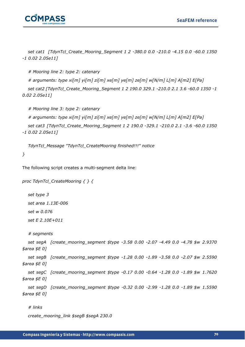
SeaFEM reference


set cat1 [TdynTcl_Create_Mooring_Segment 1 2 -380.0 0.0 -210.0 -4.15 0.0 -60.0 1350 -1 0.02 2.05e11]


# arguments: type xi[m] yi[m] zi[m] xe[m] ye[m] ze[m] w[N/m] L[m] A[m2] E[Pa]

set cat2 [TdynTcl_Create_Mooring_Segment 1 2 190.0 329.1 -210.0 2.1 3.6 -60.0 1350 -1 0.02 2.05e11]


# arguments: type xi[m] yi[m] zi[m] xe[m] ye[m] ze[m] w[N/m] L[m] A[m2] E[Pa]

set cat3 [TdynTcl_Create_Mooring_Segment 1 2 190.0 -329.1 -210.0 2.1 -3.6 -60.0 1350 -1 0.02 2.05e11]

TdynTcl_Message "TdynTcl_CreateMooring finished!!!" notice

}

The following script creates a multi-segment delta line:


set type 3

set area 1.13E-006

set w 0.076

set E 2.10E+011

# segments

set segA [create_mooring_segment $type -3.58 0.00 -2.07 -4.49 0.0 -4.78 $w 2.9370 $area $E 0]

set segB [create_mooring_segment $type -1.28 0.00 -1.89 -3.58 0.0 -2.07 $w 2.5590 $area $E 0]

set segC [create_mooring_segment $type -0.17 0.00 -0.64 -1.28 0.0 -1.89 $w 1.7620 $area $E 0]

set segD [create_mooring_segment $type -0.32 0.00 -2.99 -1.28 0.0 -1.89 $w 1.5590 $area $E 0]

# links

create_mooring_link $segB $segA 230.0

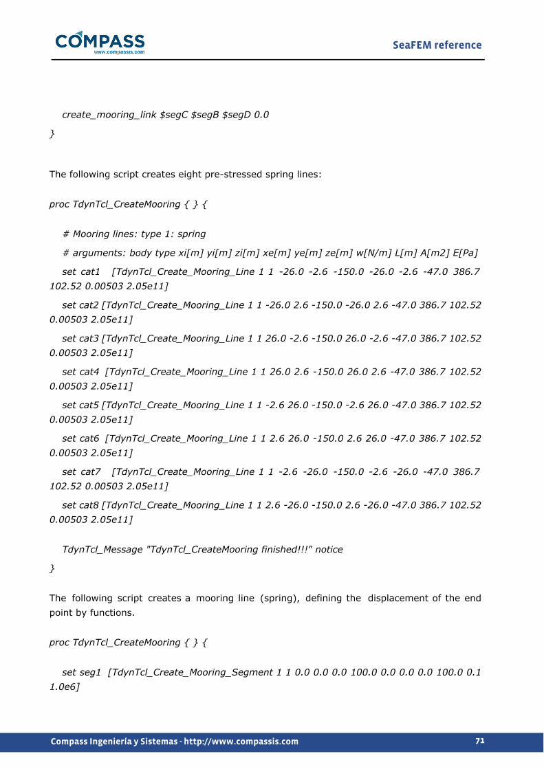
SeaFEM reference


create_mooring_link $segC $segB $segD 0.0

}

The following script creates eight pre-stressed spring lines:


# Mooring lines: type 1: spring

# arguments: body type xi[m] yi[m] zi[m] xe[m] ye[m] ze[m] w[N/m] L[m] A[m2] E[Pa]

set cat1 [TdynTcl_Create_Mooring_Line 1 1 -26.0 -2.6 -150.0 -26.0 -2.6 -47.0 386.7 102.52 0.00503 2.05e11]

set cat2 [TdynTcl_Create_Mooring_Line 1 1 -26.0 2.6 -150.0 -26.0 2.6 -47.0 386.7 102.52 0.00503 2.05e11]

set cat3 [TdynTcl_Create_Mooring_Line 1 1 26.0 -2.6 -150.0 26.0 -2.6 -47.0 386.7 102.52 0.00503 2.05e11]

set cat4 [TdynTcl_Create_Mooring_Line 1 1 26.0 2.6 -150.0 26.0 2.6 -47.0 386.7 102.52 0.00503 2.05e11]

set cat5 [TdynTcl_Create_Mooring_Line 1 1 -2.6 26.0 -150.0 -2.6 26.0 -47.0 386.7 102.52 0.00503 2.05e11]

set cat6 [TdynTcl_Create_Mooring_Line 1 1 2.6 26.0 -150.0 2.6 26.0 -47.0 386.7 102.52 0.00503 2.05e11]

set cat7 [TdynTcl_Create_Mooring_Line 1 1 -2.6 -26.0 -150.0 -2.6 -26.0 -47.0 386.7 102.52 0.00503 2.05e11]

set cat8 [TdynTcl_Create_Mooring_Line 1 1 2.6 -26.0 -150.0 2.6 -26.0 -47.0 386.7 102.52 0.00503 2.05e11]

TdynTcl_Message "TdynTcl_CreateMooring finished!!!" notice

}

The following script creates a mooring line (spring), defining the displacement of the end point by functions.


set seg1 [TdynTcl_Create_Mooring_Segment 1 1 0.0 0.0 0.0 100.0 0.0 0.0 0.0 100.0 0.1 1.0e6]

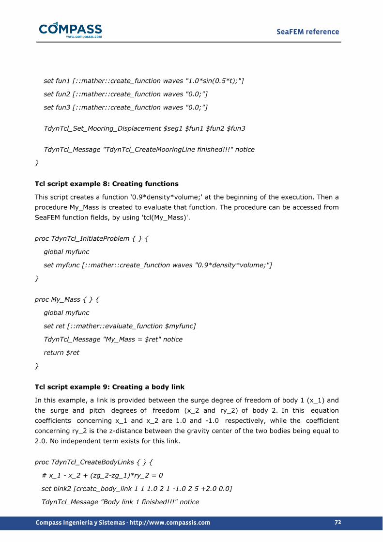
SeaFEM reference


set fun1 [::mather::create_function waves "1.0*sin(0.5*t);"]

set fun2 [::mather::create_function waves "0.0;"]

set fun3 [::mather::create_function waves "0.0;"]

TdynTcl_Set_Mooring_Displacement $seg1 $fun1 $fun2 $fun3

TdynTcl_Message "TdynTcl_CreateMooringLine finished!!!" notice

}

Tcl script example 8: Creating functions

This script creates a function '0.9*density*volume;' at the beginning of the execution. Then a procedure My_Mass is created to evaluate that function. The procedure can be accessed from SeaFEM function fields, by using 'tcl(My_Mass)'.


global myfunc

set myfunc [::mather::create_function waves "0.9*density*volume;"]

}

proc My_Mass { } {

global myfunc

set ret [::mather::evaluate_function $myfunc]

TdynTcl_Message "My_Mass = $ret" notice

return $ret

}

Tcl script example 9: Creating a body link

In this example, a link is provided between the surge degree of freedom of body 1 (x_1) and the surge and pitch degrees of freedom (x_2 and ry_2) of body 2. In this equation coefficients concerning x_1 and x_2 are 1.0 and -1.0 respectively, while the coefficient concerning ry_2 is the z-distance between the gravity center of the two bodies being equal to 2.0. No independent term exists for this link.

proc TdynTcl_CreateBodyLinks { } {

# x_1 - x_2 + (zg_2-zg_1)*ry_2 = 0

set blnk2 [create_body_link 1 1 1.0 2 1 -1.0 2 5 +2.0 0.0]

TdynTcl_Message "Body link 1 finished!!!" notice

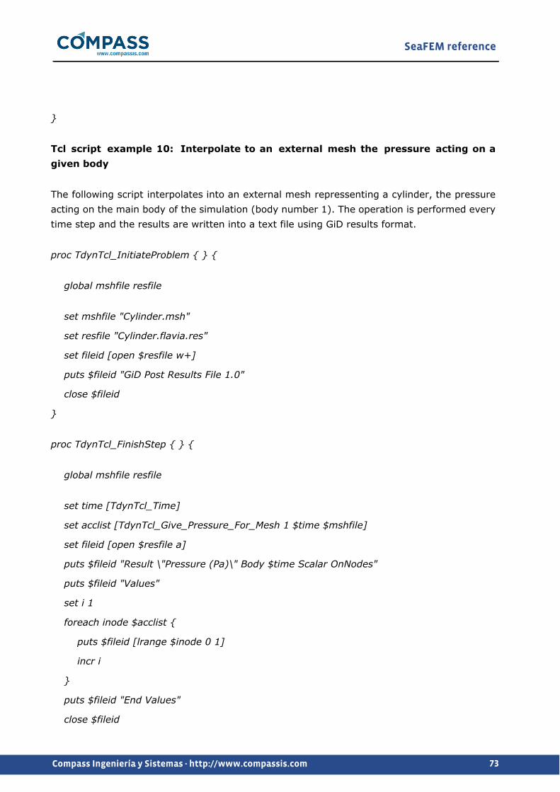
SeaFEM reference


}

Tcl script example 10: Interpolate to an external mesh the pressure acting on a given body

The following script interpolates into an external mesh repressenting a cylinder, the pressure acting on the main body of the simulation (body number 1). The operation is performed every time step and the results are written into a text file using GiD results format.


global mshfile resfile

set mshfile "Cylinder.msh"

set resfile "Cylinder.flavia.res"

set fileid [open $resfile w+]

puts $fileid "GiD Post Results File 1.0"

close $fileid

}

proc TdynTcl_FinishStep { } {

global mshfile resfile

set time [TdynTcl_Time]

set acclist [TdynTcl_Give_Pressure_For_Mesh 1 $time $mshfile]

set fileid [open $resfile a]

puts $fileid "Result \"Pressure (Pa)\" Body $time Scalar OnNodes"


set i 1


puts $fileid [lrange $inode 0 1]

incr i

}


close $fileid

SeaFEM reference


}

Tcl script example 11: Defining a mass matrix

The following script illustrates how to define the mass matrix of a body taking a generic point as the reference point for that matrix. Note that the mass matrix can be directly introduced within the graphic user interface of SeaFEM only in the case the matrix is known for the center of gravity. Hence, the tcl script procedure is usefull when the mass matrix is known from a generic reference point that may differ from the center of gravity. If this is the case, the mass matrix in the graphic user interface is left empty an the following tcl script is used to set up the mass matrix for the generic reference point. SeaFEM takes care of transforming the mass matrix from the reference point specified in the tcl script to the center of gravity or any other generic point specified for the sake of output in the user interface. In the present example, the generic point from which the mass matrix is specified is the point of coordinates (15, -25, -7). The first argument in the TdynTcl_Add_Mass_Matrix procedure indicates that the specified mass matrix concerns body number 1.


TdynTcl_Add_Mass_Matrix 1 [list 15 -25 -7] [list \

1607.95 0 0 0 11255.65 -40198.75 \

0 1607.95 0 -11255.65 0 -24119.25 \

0 0 1607.95 40198.75 24119.25 0 \

0 -11255.65 40198.75 1085366 602981 168835 \

11255.65 0 24119.25 602981 442186.3 -281391.3 \

-40198.75 -24119.25 0 168835 -281391.3 1368365 ]

TdynTcl_Message "TdynTcl_InitiateProblem finished!!!" notice

}

Appendix C: RAO analysis

When carrying out RAO analysis using the white noise spectrum, it must be taken into account that the SeaFEM RAO's calculation is based on a discret Fourier transform decomposition. Because of this, the total calculation time and the sampling time are automatically calculated and fixed internally by the solver based on the maximum and the minimum frequencies (periods) specified by the user in the graphic user interface. Hence, even if a "Simulation time" and/or a "Time step" are specified by the user, they will be ignored and fixed internally by SeaFEM. Only the "Initialization time" parameter will maintained since it can be usefull to avoid energetic transient. This is because a sudden initialization (which can occur when no initialization time is specified) might lead to large accumulation of energy by the body, which would require longer simulation to dissipate all

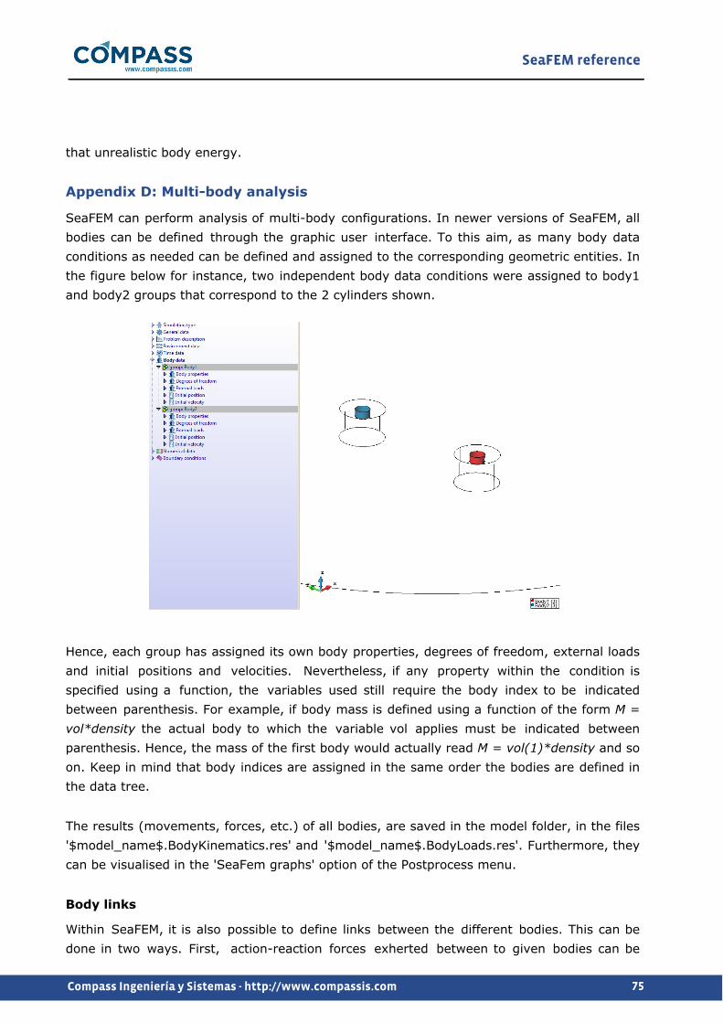
SeaFEM reference


that unrealistic body energy.

Appendix D: Multi-body analysis

SeaFEM can perform analysis of multi-body configurations. In newer versions of SeaFEM, all bodies can be defined through the graphic user interface. To this aim, as many body data conditions as needed can be defined and assigned to the corresponding geometric entities. In the figure below for instance, two independent body data conditions were assigned to body1 and body2 groups that correspond to the 2 cylinders shown.

Hence, each group has assigned its own body properties, degrees of freedom, external loads and initial positions and velocities. Nevertheless, if any property within the condition is specified using a function, the variables used still require the body index to be indicated between parenthesis. For example, if body mass is defined using a function of the form M = vol*density the actual body to which the variable vol applies must be indicated between parenthesis. Hence, the mass of the first body would actually read M = vol(1)*density and so on. Keep in mind that body indices are assigned in the same order the bodies are defined in the data tree.

The results (movements, forces, etc.) of all bodies, are saved in the model folder, in the files '$model_name$.BodyKinematics.res' and '$model_name$.BodyLoads.res'. Furthermore, they can be visualised in the 'SeaFem graphs' option of the Postprocess menu.

Body links

Within SeaFEM, it is also possible to define links between the different bodies. This can be done in two ways. First, action-reaction forces exherted between to given bodies can be

SeaFEM reference


introduced as external loads acting on the corresponding bodies. These functions use the standard syntax shown in section Appendix A: function editor -pag. 45-, but it is extended for multi-bodies analysis, by adding the index of the body between parenthesis at the end of the function. The following are some examples of this extension:

mass(2): mass of the body of index 2.dx[1.0,1.0,1.0](1): displacement of the point 1.0,1.0,1.0 of the body of index 1.yg(3): Y coordinate of the center of graity of the body of index 3.

Secondlly, links can also be created that correlate degrees of freedom from different bodies. This is internally implemented by using a Lagrange's multipliers approach. This essentially consists on adding a matrix of restrictions to the bodies dynamics, each row of that matrix corresponding to the equation defining a link. At the user's level, it is necessary to define these kind of links by using a tcl script procedure. In particular, a Tcl procedure named TdynTcl_CreateBodyLinks must be reimplemented by the user in the tcl script. Within these procedure, several types of joints between bodies (each implying different number of body links) can be defined following the sintax detailed below. In addition, body links can be optionally updated at each iteration to take into account large displacements and rotations. To this aim, a Tcl procedure named TdynTcl_StartNewIteration must be reimplemented by the user in the tcl script. The sintax of the tcl functions used to update the joints (links) is identical to their creation counterpart just adding a first argument to identify the constraint equation index to be updated.

The type of body joints currently available within SeaFEM is listed bellow:

Rotation constraintLine constraintPlane constraintRotation linkTranslation linkRigid body jointBall jointRevolute jointCylindrical jointPrismatic joint

Next, the above body constraints and mechanical joints are described in detail alongside with the arguments required to define each one of the body link relations.

Rotation constraint

This type of constraint is used to prevent body rotation around an arbitrary given direction.

SeaFEM reference


create_rotation_constraint #body #a #b #cupdate_rotation_constraint #ilink #body #a #b #c

Argument #body1 must be an integer value (greatter than 0) and is used to identify the body affected by the rotation constraint. Such an index must respond to the order of creation of the bodies in the interface. Arguments #a #b #c are the direction cosines

of the axis about which the rotation ob the body is prevented.

Line constraint

This type of constraint is used to enforce body movement along a given direction (the body is allowed to move only

along a given direccion.

create_line_constraint #body #a #b #cupdate_line_constraint #ilink #body #a #b #c

Argument #body1 must be an integer value (greatter than 0) and is used to identify the body affected by the line constraint. Such an index must respond to the order of creation of the bodies in the interface. Arguments #a #b #c are the direction cosines

of the direction along which the body can move.

Plane constraint

This type of constraint is used to enforce body movement over a given plane. The body is allowed to move only over a plane whose normal is given and going through the initial position of the body's reference point.

create_plane_constraint #body #a #b #cupdate_plane_constraint #ilink #a #b #c

Argument #body1 must be an integer (greater than 0) and is used to identify the body to which the plane constraint applies. This body index must be consistent with the order of creation of the bodies in the user interface. Arguments #a #b #c are the direction cosines of the plane's normal direction.

Rotation link

This type of joint is used to enforce the rotation degree of freedom of two different bodies to be the same.

SeaFEM reference


create_rotation_link #body1 #body2 #rotdofupdate_rotation_link #ilink #body1 #body2 #rotdof

Arguments #body1 and #body2 must be integer values greater than 0 and are used to identify the two bodies being joined by the rotation link. These indexes correspond to the order of creation of the bodies in the interface. Argument #rotdof must be an integer value between 1 and 3 and is used to identify the constrained rotational degree of freedom (1 = Roll, 2 = Pitch, 3 = Yaw). Argument #ilink identifies the constraint equation index to be updated. It usually corresponds to an integer variable previously initialized by the return value of the create_link function.

Translation link

This type of link is used to create a constraint between translational degrees of freedom of 2 bodies.

create_translation_link #body1 #body2 #transdofupdate_translation_link #ilink #body1 #body2 #transdof

Arguments #body1 and #body2 must be integer values (greater than 0) and are used to identify the two linked bodies. These indexes correspond to the order of creation the different bodies in the interface. Argument #transdof must be an integer value between 1 and 3 and is used to identify the constrained translational degree of freedom (1 = Surge, 2 = Sway, 3 = Heave). Argument #ilink identifies the constraint equation index to be updated. It usually corresponds to an integer variable previously initialized by the return value of the create_link function.

Rigid body joint

This type of joint can be used to enforce two different bodies to move as a single rigid body. The advantage of modelling the rigid body as two separate components instead of a unique body, is that forces and moments exherted by one component over the other are then accessible in the form of body joint reactions.

create_rigid_body_full_link #body1 #body2update_rigid_body_full_link #ilink #body1 #body2

Arguments #body1 and #body2 must be integer values greater than 0 and are used to identify the two components of the rigid body set. These indices must correspond to the order the bodies were created in the user interface. Argument #ilink identifies the constraint equation index to be updated. It usually corresponds to an integer variable previously initialized by the

SeaFEM reference


return value of the create_link function.

Ball joint

This type of link is used to create a ball joint constraint between 2 bodies. This means that the two bodies being joined share a common point (usually the ball joint position point) about which both bodies can rotate freely.

create_ball_joint_link #body1 #body2 #x #y #zupdate_ball_joint_link #ilink #body1 #body2 #x #y #z

Arguments #body1 and #body2 must be integer values greater than 0 and are used to identify the two linked bodies. These indexes correspond to the order of creation of the different bodies in the interface.Arguments #x, #y and #z must be real values that define the initial global position of the ball joint. Argument #ilink identifies the constraint equation index to be updated. It usually corresponds to an integer variable previously initialized by the return value of the create_link function.

Revolute joint

This type of joint is used to create a revolute constraint between 2 bodies. This type of junction implies that the two bodies can freely rotate about a common axis (actually the bodies share two points aligned on a given axis), while the remaining degrees of freedom (translation and rotation) are linked.

create_revolute_joint_link #body1 #body2 #x1 #y1 #z1 #x2 #y2 #z2update_revolute_joint_link #ilink #body1 #body2 #x1 #y1 #z1 #x2 #y2 #z2

Arguments #body1 and #body2 must be integer values greater than 0 and are used to identify the two bodies joined through the revolute joint. These indexes correspond to the order of creation of the different bodies in the interface. Arguments #x1, #y1, #z1 and #x2, #y2, #z2 must be real values defining the two points shared by the bodies. Actually these points define the common axis of revolution.

Cylindrical joint

This type of link is used to create a cylindrical joint between 2 bodies. A cylindrical joint implies that the two bodies can undergo relative translation along a given axis and relative rotation about the same axis. All the remaining degrees of freedom are linked.

create_cylindrical_joint_link #body1 #body2 #a #b #c

SeaFEM reference


update_cylindrical_joint_link #ilink #body1 #body2 #x #y #z

Arguments #body1 and #body2 must be integer values greater than 0 and are used to identify the two bodies linked by the cylindrical joint. These indexes correspond to the order of creation of the different bodies in the interface. Arguments #a #b and #c must be real values that define the vector/axis that characterizes the cylindrical joint. Argument #ilink identifies the constraint equation index to be updated. It usually corresponds to an integer variable previously initialized by the return value of the create_link function.

Prismatic joint

This type of link is used to create a prismatic joint constraint between 2 bodies. A prismatic joint means that all rotational degrees of freedom are linked (this is, both bodies undergo identical roll, pitch and yaw rotations) and that both bodies can undergo relative translation only along a given axis.

create_prismatic_joint_link #body1 #body2 #a #b #cupdate_prismatic_joint_link #ilink #body1 #body2 #a #b #c

Arguments #body1 and #body2 must be integer values greater than 0 and are used to identify the two joined bodies. These indexes correspond to the order of creation the different bodies in the interface. Arguments #a #b and #c must be real values that define the axis along which the two bodies can undergo relative displacement. Argument #ilink identifies the constraint equation index to be updated. It usually corresponds to an integer variable previously initialized by the return value of the create_link function.

An example of tcl script procedure reads as follows:

proc TdynTcl_CreateBodyLinks { } { global link1 link2 set link1 [create_ball_joint_link 1 2 0.0 0.0 -1.0] set link2 [create_rotation_link 1 2 0]}

proc TdynTcl_StartNewIteration { } { global link1 link2 update_ball_joint_link $link1 1 2 0.0 0.0 -1.0 update_rotation_link $link2 1 2 0}

SeaFEM reference


In this example, first a ball joint link is created between bodies 1 and 2 (the corresponding equation index is stored in the global variable link1). The ball joint is located at the position given by the initial global coordinates 0.0, 0.0, -1.0. Secondly, an additional constraint between bodies 1 and 2 is created so that both bodies rigidly rotate in roll direction (link 2).

Generic links can also be created that correlate any number of degrees of freedom from different bodies. The implementation of this kind of links essentially consists on calling the TdynTcl_Create_Body_Link function through the Tcl script. The arguments passed to this function are triads of values that consecutively define the various coefficients of the particular link equation. To this aim, each triad consists on an integer identifying the body, another integer identifying the degree of freedom and a real value setting the corresponding coefficient value. An additional argument can be provided at the end to specify an optional independent coefficient that could exist for a given link equation. An example of tcl script procedure for this kind of generic link would read as follows:

proc TdynTcl_CreateBodyLinks { } {# x_1 - x_2 + (zg2 - zg1)*ry_2 = 0TdynTcl_Create_Body_Link 1 1 1.0 2 1 -1.0 2 5 2.0 0.0

}

In this example, a link is provided between the surge degree of freedom of body 1 and the surge degree of freedom of body 2. In this equation, coefficients concerning x_1 and x_2 are 1.0 and -1.0 respectively, while the coefficient concerning ry_2 is the z-distance between the gravity center of the two bodies (zg2 - zg1) being equal to 2.0. No independent term exists for this link.

It is also possible to define links between bodies using the different mooring options of SeaFEM. See Appendix E: Mooring definition by Tcl -pag. 81- section for further information.

Appendix E: Mooring definition by Tcl

Mooring definition in SeaFEM can be done by using the GUI options available (see Mooring data -pag. 28- section for further information). However, mooring systems can also be defined through a Tcl script procedure, that gives access to advanced mooring definition options. The Tcl procedure must be implemented in a text file. Such a file, is further provided as an input argument of the Tcl data section of the data tree, once the option to use an external Tcl script is activated.

SeaFEM reference


Tcl data section of the SeaFEM data tree

Tcl data can be accessed and modified at any time through the menu option:

General data Tcl data

The procedure to be implemented in the tcl script is named TdynTcl_CreateMooringLine and simply consists on the definition of all mooring segments and further definition of the segment links. Segments definition is performed by calling the SeaFEM internal function create_mooring_segment. Arguments passed to this function are described below. Links between segments are specified by calling the SeaFEM internal function create_mooring_link. Arguments passed to this function are also described below.

The syntax to call TdynTcl_Create_Mooring_Segment and the arguments passed to the function are as follows:

syntax : TdynTcl_Create_Mooring_Segment $body $type $xi $yi $zi $xe $ye $ze $w $L $A $E [$S $N $d1 $d2]

alternative syntax: create_mooring_segment $body $type $xi $yi $zi $xe $ye $ze $w $L $A $E [$S $N $d1 $d2]

The arguments between brackets only apply to certain types of mooring segments.

body : index of the body which the mooring is linked to (from 1 to n). If no body is specified, the current mooring segment is assumed to be attached to the main bodytype : this parameter determines the type of mooring segment to be used. The possible values of this parameter are:

SeaFEM reference


type = 1 - quasi-static elastic bar (spring able to work in both, tension and compression regimes). type = 2 - quasi-static catenary type = 3 - quasi-static cable (spring able to work only in tension) type = 4 - quasi-static elastic catenary type = 6 - dynamic cable

xi [m] : x coordinate of the initial point of the mooring segment (this must be the point closer to the body)yi [m] : y coordinate of the initial point of the mooring segment (this must be the point closer to the body)zi [m] : z coordinate of the initial point of the mooring segment (this must be the point closer to the body)xe [m] : x coordinate of the end point of the mooring segmentye [m] : y coordinate of the end point of the mooring segmentze [m] : z coordinate of the end point of the mooring segmentw [N/m] : effective weight (actual weight minus bouyancy) per unit lengthL [m] : length of the segmentA [m2] : cross section area of the cableE [Pa] : Young modulusS : this is the seabed parameter. This argument has only effect for catenary (type 2) and elastic catenary (type 4) segments. If it is provided for other mooring types, it will be actually ignored. The possible values of this parameter are:

S = 0 - the catenary is fixed to a seabed point S > 0 - the catenary rests on the seabed. In case of elastic catenary, S = 1 considers a sandy seabed contact, S = 2 considers a sliding seabed wire, and S = 3 considers a sliding seabed chain.

N : This argument only applies in the case of dynamic cables (type 6). It indicates the number of line elements for cable geometric discretization.d1, d2 : User defined damping ratios.

For each segment, initial and end points must be introduced in a specific order, being the initial point the closest one to the body. The function simply returns an identifier for the created segment, that can be used to define links among the different mooring segments. These links are defined using the function create_mooring_link, as defined in the following.

By default, create_mooring_segment assumes that the initial point is linked to the given body, and the end point is fixed at the seabed. However, this assumption can be overwritten by defining links with other mooring segments or bodies. As commented above, the function create_mooring_link can be used to define links among the different segments of a multi-segment mooring line. This function can create different type of links as explained below.

SeaFEM reference


The syntax to call create_mooring_link and the arguments passed to the function are as follows:

syntax : create_mooring_link $seg1 $seg2 $f

alternative syntax: TdynTcl_Create_Mooring_Link $seg1 $seg2 $f

seg1 : identifier variable corresponding to the first segment of the link (this must be the segment closer to the body)seg2 : identifier variable corresponding to the second segment of the linkf [N] : buoyancy force to be applied at the link node

The operator TdynTcl_Create_Mooring_Link can also be used to define links between three lines (joint to the same node). In that case, the syntax of the function is as follows:

syntax : TdynTcl_Create_Mooring_Link $seg1 $seg2 $seg3 $f

alternative syntax: create_mooring_link $seg1 $seg2 $seg3 $f

seg1 : identifier variable corresponding to the first segment of the link (the segment closer to the body)seg2 : identifier variable corresponding to the second segment of the linkseg3 : identifier variable corresponding to the third segment of the linkf [N] : buoyancy force to be applied at the link node

The function TdynTcl_Create_Mooring_Link can also be used to define links between two bodies. In that case, the syntax of the function is as follows:

syntax : TdynTcl_Create_Mooring_Link $seg1 &body

alternative syntax: create_mooring_link $seg1 &body

seg1 : identifier variable corresponding to the segment of the linkbody : index of the body which the mooring is linked to (from 1 to n).

An example of a TCL script for defining a multi-catenary mooring system is shown below. It corresponds to the mooring system configuration sketched in the following figure:

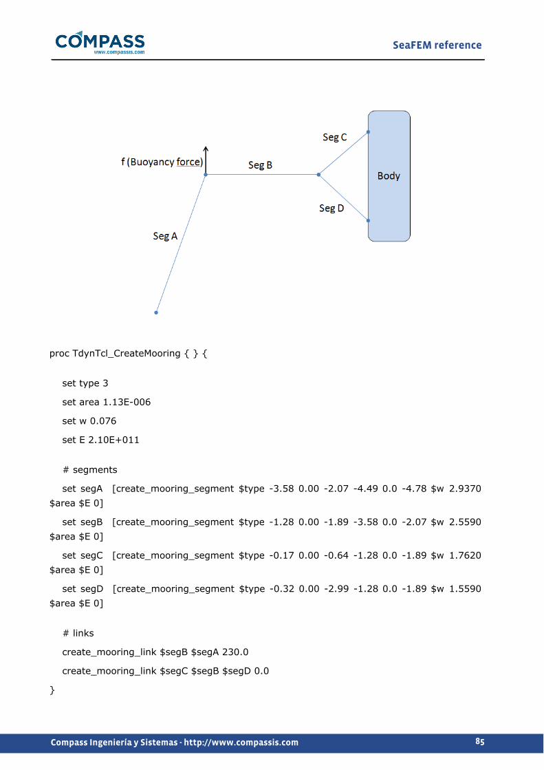
SeaFEM reference



set type 3

set area 1.13E-006

set w 0.076

set E 2.10E+011

# segments

set segA [create_mooring_segment $type -3.58 0.00 -2.07 -4.49 0.0 -4.78 $w 2.9370 $area $E 0]

set segB [create_mooring_segment $type -1.28 0.00 -1.89 -3.58 0.0 -2.07 $w 2.5590 $area $E 0]

set segC [create_mooring_segment $type -0.17 0.00 -0.64 -1.28 0.0 -1.89 $w 1.7620 $area $E 0]

set segD [create_mooring_segment $type -0.32 0.00 -2.99 -1.28 0.0 -1.89 $w 1.5590 $area $E 0]

# links

create_mooring_link $segB $segA 230.0

create_mooring_link $segC $segB $segD 0.0

}

SeaFEM reference


The function TdynTcl_Set_Mooring_Displacement can be used to define the displacement of the end point of a mooring segment.

syntax : TdynTcl_Set_Mooring_Displacement $seg1 $fun1 $fun2 $fun3

alternative syntax: set_mooring_displacement $seg1 $fun1 $fun2 $fun3

seg1 : identifier variable corresponding to the segmentfun1 : index of the function describing the time-dependent displacement in OX of the end point of the mooring segmentfun2 : index of the function describing the time-dependent displacement in OY of the end point of the mooring segmentfun3 : index of the function describing the time-dependent displacement in OZ of the end point of the mooring segment

The function TdynTcl_Configure_Mooring_Segment can be used to configure advanced options of the cable segments.

syntax : TdynTcl_Configure_Mooring_Segment $seg1 $Gk $Gc $Gu $Cd $Cf $Cm $alpha $bci

alternative syntax: configure_moorin_segment $seg1 $Gk $Gc $Gu $Cd $Cf $Cm $alpha $bci

seg1 : identifier variable corresponding to the segmentGk : ground normal stiffness per unit length (Pa/m) for seabed interactionGc : ratio of critical damping of ground (-) for seabed interactionGu : friction coefficient (-) for seabed interactionCd : tangential drag coeficient of the cableCf : normal drag coeficient of the cableCm : added mass coefficient of the cablealpha : Alpha coefficient of the Bossak-Newmark integration schemebci : boundary condition for the initial node: 1 if acceleration is imposed, -1 if the node is

Visualization of mooring results

When running a SeaFEM analysis that includes mooring lines defintion, specific result files are generated concerning the mooring system:

MooringLoads.res - It contains the forces and moments exherted by the mooring system on the attached body. MooringResults.msh - It contains an authomatically generated mesh of the mooring system. MooringResults.res - It contains the displacement results of each mooring segment. projectName.MooringData.res - It contains the tension force components at both ends of each mooring segment.

SeaFEM reference


If MooringResults.msh and MooringResults.res files exist, they are authomatically loaded into the postprocessor graphic user interface. All mooring segments appear grouped within a single Mesh group called "Mooring". Visualization options of each mooring segment can be manipulated individually as can be done with any other mesh. Mooring displacement results can also be animated by drawing the corresponding deformed result as shown in the figure below. To this aim, follow the steps listed in what follows:

1 - In the meshes window, check all mooring segments that you want to be plotted.2 - Select the "Mooring > Displacement > Contour fill" option in the results window.3 - Choose the "Deformed > Result > Mooring {Displacement}" option in the preferences

window.4 - Finally, activate the "Deformed > Draw" option in the preferences window.

Appendix F: Morison's forces effect

When viscous effects may be advanced to have a significant effect on the dynamic behavior of an offshore structure, Morison's equation can be used to correct the forces evaluated by the difraction-radiation solver. For this purpose, an auxiliary framework structure, associated to a body must be defined. Based on the information provided by the user, SeaFEM evaluates Morison's forces per unit length acting on this framework structure. After integration along the different elements, the resultant forces are incorporated to the dynamic solver of the rigid body to which the idealized framework structure has been associated.

To this aim, a tcl procedure must be used to define the different elements of the framework structure associated to a body. This procedure allows specifying the reference line of the element as well as the added mass, lift, drag and friction coefficients of the Morison's

SeaFEM reference


equation. This function can be called several times to define as many elements as required.

The syntax to define the Tcl procedure to create new elements of the framework structure read as follows:

TdynTcl_Add_Morison_Element b t x1 y1 z1 x2 y2 z2 D S CM CD CV CF CL

where:

b is and integer index that identifies the body to which the Morison element pertains,t is the element type (1 defines a standard element for which the floatability forces are evaluated, and 2 defines a virtual element for which floatability forces are neglected).x1, y1, z1, x2, y2, z2 are the coordinates of the end points of the cylinder,D is the section characteristic linear dimension (the diameter in the case of a cylinder),S is the cross section area,CM is the added mass correction coefficient,

CD is the non-linear drag coefficient,

CV is the linear drag coefficient,

CF is the friction coefficient,

and CL is the lift coefficient.

TdynTcl_Add_Morison_Element procedure returns the index of the created element of the framework structure.

Based on the information provided in the succesive calls to TdynTcl_Add_Morison_Element command, SeaFEM evaluates Morison's forces per unit length acting on the framework structure defined by the suer. After integration, the resultant forces are incorporated to the dynamics of the rigid body to which the framework structure has been associated. The various (per unit length) contributions to the force are calculated as follows:

FM= CM·ρ·S·(lxaxl)

FD= 0.5·CD·ρ·D|lxvxl|(lxvxl)

FV= 0.5·CV·ρ·D·(lxvxl)

FF= 0.5·CF·ρ·π·D|l·v|(l·v)·l

FL= 0.5·CL·ρ·D|lxv|(lxv)

where l is the unit vector locally oriented along the element, a is the relative acceleration vector, v is the relative velocity vector, and FM, FD, FV, FF and FL are the inertial correction,

drag, linear drag, friction and lift components of the force per unit length respectively.

Remark: If the defined CM coefficient is greater than 1, then FM component is evaluated in

SeaFEM reference


the following alternative way:

FM=(CM-1)·ρ·S·(lxaxl))+ρ·S·(lxawxl)

where aw is the fluid acceleration of the incident wave, and therefore, the second term in the

right hand side of the above equations represents the Froude-Kriloff force.

It is important to keep in mind that the added mass contribution calculated using the Morison's equation will be added to the added mass effect that is already accounted for by the diffraction-radiation SeaFEM solver. Hence, the added mass contribution of the Morison's equation must be only used if, for some reason, the user wishes to correct the added mass effect calculated by SeaFEM.

It is emphasized that SeaFEM will always calculate the inertia term by integrating the pressure field on the body surface. This will result in the evaluation of the Froude-Krylov force plus diffraction force. On the other hand, it is well known that viscous effects can reduce the amplitude of the diffraction force, and in most of the cases SeaFEM calculation will result in overprediction of this value. Hence, the added mass contribution of the Morison's equation can be used to improve the computational prediction of this force, by setting a suitable (usually negative) value of CM, based on experimental information.

As an example, the following code can be used to add to body number 1 the Morison forces acting on a cylinder whose axis is oriented in the vertical z-direction. In this simplified example, only added mass and non-linear drag effects are considered, while linear drag, friction and lift corrections are kept null.

proc TdynTcl_StartSetProblem {} { set idx [TdynTcl_Add_Morison_Element 1 0 0.0 0.0 0.0 0.0 0.0 -0.5 1 0.7854 -0.3 1.4 0.0 0.0 0.0]}

Finally, it is possible to update the values of the different coefficients of an element of the auxiliary framework structure. The syntax of the Tcl procedure that can be used for this purpose read as follows:

TdynTcl_Update_Morison_Element idx CM CD CV CF CL

where:

idx index of the previously created element of the framework structure (returned by TdynTcl_Add_Morison_Element),CM is the updated added mass correction coefficient,

SeaFEM reference


CD is the updated non-linear drag coefficient,

CV is the updated linear drag coefficient,

CF is the updated friction coefficient,

and CL is the updated lift coefficient.

As an example, the following code can be used to nullify the Morison's correction of the framework element of index 1, after 1.0 s of simulation.

As an example, the following code can be used to nullify the Morison's correction of the framework element of index 1, after 1.0 s of simulation.

proc TdynTcl_StartNewStep {} {

if {[TdynTcl_Time]>1.0} {

TdynTcl_UpdateAdd_Morison_Element 1 0.0 0.0 0.0 0.0 0.0

}

}

As stated above, the forces evaluated on the auxiliary framework structure are added to the dynamic solver of the different associated bodies. Furthermore, these forces are outputed to the ASCII file 'MorisonLoads.res'. This file constains 24·n columns, where n is the number of bodies in the analysis. For every body, the following 24 values are written every time step:

Mx: X component of the added mass force acting on the center of gravity of the body. My: Y component of the added mass force acting on the center of gravity of the body. Mz: Z component of the added mass force acting on the center of gravity of the body. MMx: X component of the added mass moment acting on the center of gravity of the body. MMy: Y component of the added mass moment acting on the center of gravity of the body. MMz: Z component of the added mass moment acting on the center of gravity of the body. Dx: X component of the total drag force acting on the center of gravity of the body. Dy: Y component of the total drag force acting on the center of gravity of the body. Dz: Z component of the total drag force acting on the center of gravity of the body. DMx: X component of the total drag moment acting on the center of gravity of the body. DMy: Y component of the total drag moment acting on the center of gravity of the body. DMz: Z component of the total drag moment acting on the center of gravity of the body. Fx: X component of the friction force acting on the center of gravity of the body. Fy: Y component of the friction force acting on the center of gravity of the body. Fz: Z component of the friction force acting on the center of gravity of the body. FMx: X component of the friction moment acting on the center of gravity of the body. FMy: Y component of the friction moment acting on the center of gravity of the body. FMz: Z component of the friction moment acting on the center of gravity of the body.

SeaFEM reference


Lx: X component of the lift force acting on the center of gravity of the body. Ly: Y component of the lift force acting on the center of gravity of the body. Lz: Z component of the lift force acting on the center of gravity of the body. LMx: X component of the lift moment acting on the center of gravity of the body. LMy: Y component of the lift moment acting on the center of gravity of the body. LMz: Z component of the lift moment acting on the center of gravity of the body.

Appendix G: Analysis advanced configuration

Several advanced (or rarely used) options of the analysis can be configured through the Tcl extension of SeaFEM. As usual, the necessary tcl script procedure must be implementd in a text file, which is further provided as an input argument in the Tcl data section of the data tree once the option to use an external Tcl script is activated.

General data Tcl data

The specification of advanced options is performed by reimplementing the TdynTcl_InitiateProblem procedure, and simply consists on calling the SeaFEM internal function configure_analysis with two arguments indicating the advanced option's name and the corresponding value. Available configuration options are described in the following list:

Mooring_Elements_Number: sets the number of elements for the output of dynamic mooring results. The second argument must be a positive integer number.Mooring_Initial_Damping: activates or deactivates the initial damping for dynamic mooring. The second argument must be 0 (deactivated) or 1 (activated).Mooring_Solver_Type: sets the type of nonlinear solver for dynamic mooring lines. The remaining arguments must be a couple of real values.Morison_Elements_Number: sets the number of elements for the output of Morison element results. The second argument must be a positive integer number.Relax_Type: switchs on and off the Aitkens relaxation method for wave-structure coupling analysis. The second argument must be 0 (deactivated) or 1 (activated).Solve_Dif_Rad: switchs on and off the diffraction-radiation solver. The second argument must be 0 (switch off) or 1 (switch on).Moving_frame: updates the cordinates reference frame according to the main body horizontal displacement. The second argument must be 0 (deactivated) or 1 (activated).

Example: the following Tcl script can be used to deactivate the solution of the diffraction-radiation problem (so that only incident waves are taken into account) and to update the coordinates reference frame in accordance to the horizontal displacement og the main body.


SeaFEM reference


configure_analysis Solve_Dif_Rad 0

configure_analysis Moving_frame 1

}

SeaFEM reference - Compass Webpage - Home€¦ · · 2015-06-29SeaFEM reference Compass...

Documents

Transcript of SeaFEM reference - Compass Webpage - Home€¦ · · 2015-06-29SeaFEM reference Compass...