
SDOF review 061904 - Faculty Server Contact | UMass...
34
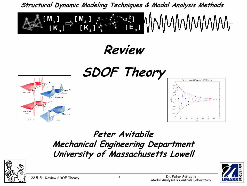
1 Dr. Peter Avitabile Modal Analysis & Controls Laboratory 22.515 – Review SDOF Theory Review SDOF Theory Peter Avitabile Mechanical Engineering Department University of Massachusetts Lowell [ K ] n [ M ] n [ M ] a [ K ] a [ E ] a [ ω ] 2 Structural Dynamic Modeling Techniques & Modal Analysis Methods
Transcript of SDOF review 061904 - Faculty Server Contact | UMass...
1 Dr. Peter AvitabileModal Analysis & Controls Laboratory22.515 – Review SDOF Theory
Review SDOF Theory
Peter AvitabileMechanical Engineering DepartmentUniversity of Massachusetts Lowell
[ K ]n
[ M ]n [ M ]a[ K ]a [ E ]a
[ ω ]2
Structural Dynamic Modeling Techniques & Modal Analysis Methods
2 Dr. Peter AvitabileModal Analysis & Controls Laboratory22.515 – Review SDOF Theory
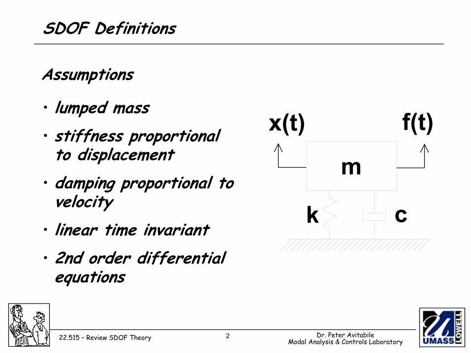
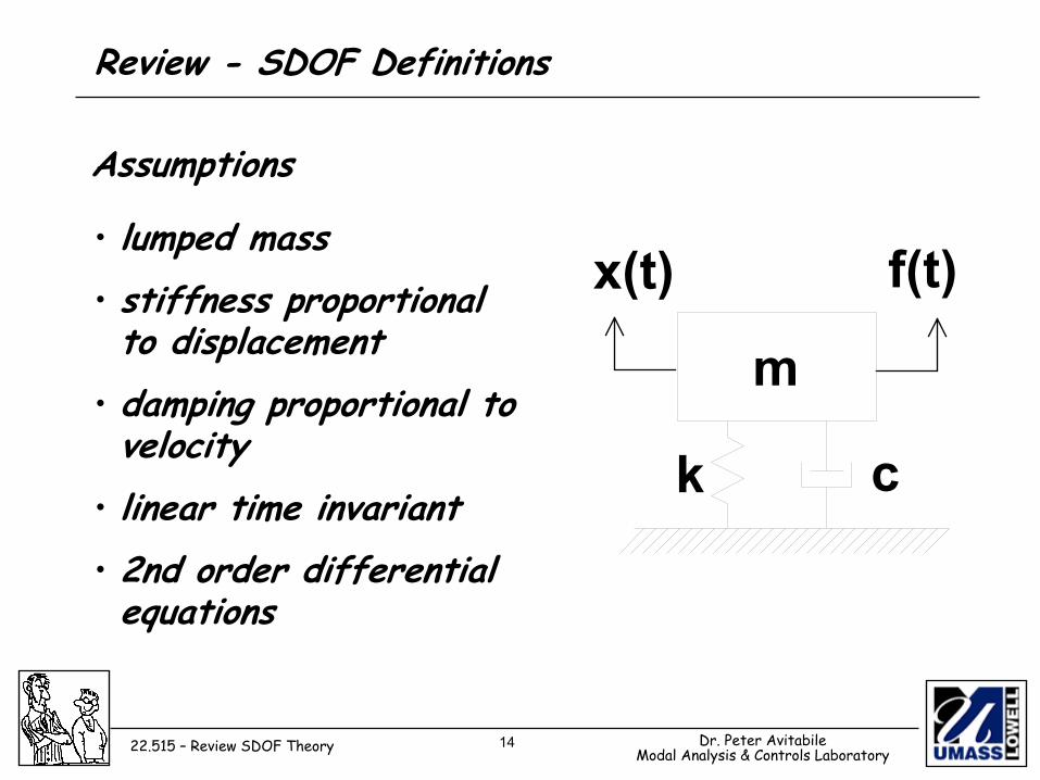
SDOF Definitions
• lumped mass• stiffness proportional to displacement
• damping proportional to velocity
• linear time invariant• 2nd order differential equations
Assumptions
m
k c
x(t) f(t)
3 Dr. Peter AvitabileModal Analysis & Controls Laboratory22.515 – Review SDOF Theory
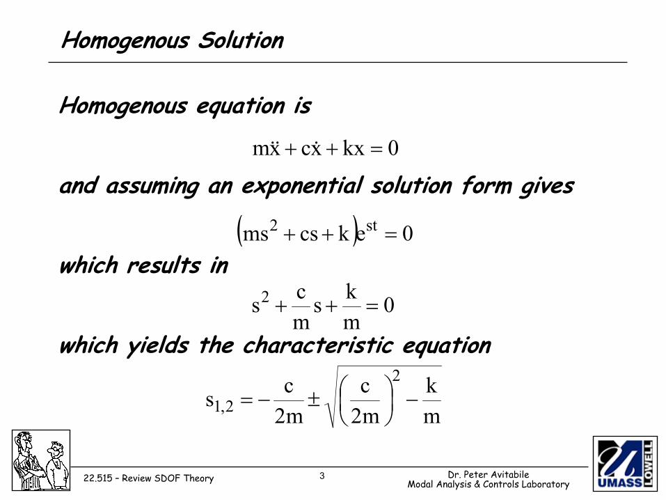
Homogenous Solution
Homogenous equation is
and assuming an exponential solution form gives
which results in
which yields the characteristic equation
0kxxcxm =++ &&&
( ) 0ekcsms st2 =++
0mks
mcs2 =++
mk
m2c
m2cs
2
2,1 −
±−=
4 Dr. Peter AvitabileModal Analysis & Controls Laboratory22.515 – Review SDOF Theory
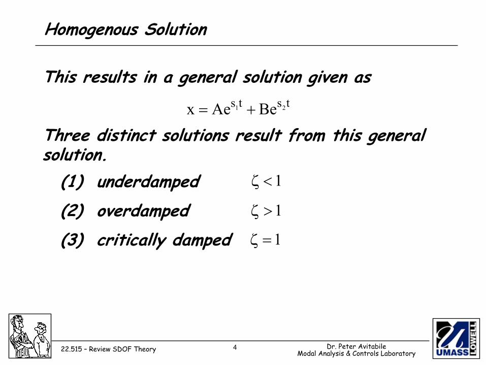
Homogenous Solution
This results in a general solution given as
Three distinct solutions result from this general solution.
tsts 21 BeAex +=
(1) underdamped(2) overdamped(3) critically damped
1<ζ
1>ζ
1=ζ
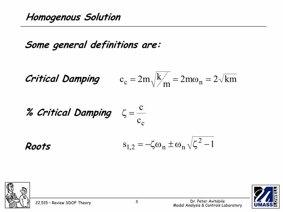
5 Dr. Peter AvitabileModal Analysis & Controls Laboratory22.515 – Review SDOF Theory
Homogenous Solution
Some general definitions are:
Critical Damping
% Critical Damping
Roots
km2m2mkm2c nc =ω==
ccc
=ζ
1s 2nn2,1 −ζω±ζω−=
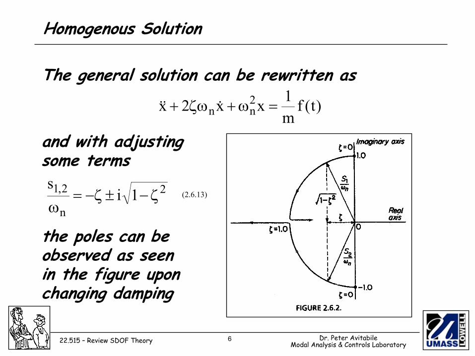
6 Dr. Peter AvitabileModal Analysis & Controls Laboratory22.515 – Review SDOF Theory
The general solution can be rewritten as
and with adjustingsome terms
the poles can be observed as seen in the figure uponchanging damping
(2.6.13)
Homogenous Solution
)t(fm1xx2x 2
nn =ω+ζω+ &&&
2
n
2,1 1is
ζ−±ζ−=ω
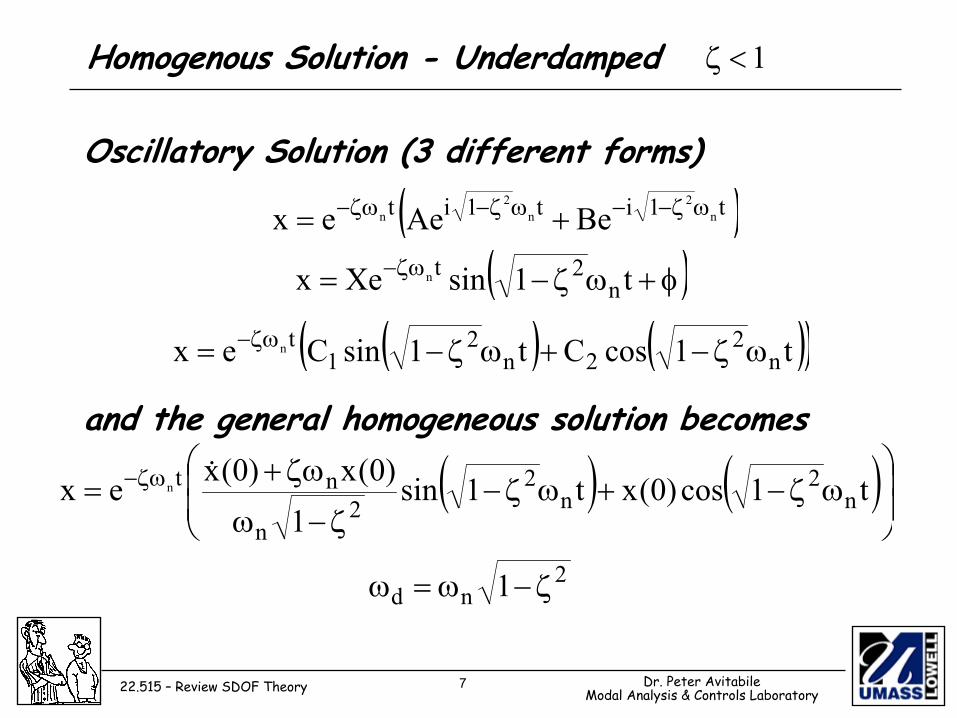
7 Dr. Peter AvitabileModal Analysis & Controls Laboratory22.515 – Review SDOF Theory
Oscillatory Solution (3 different forms)
and the general homogeneous solution becomes
Homogenous Solution - Underdamped 1<ζ
( )t1it1it n2
n2
n BeAeex ωζ−−ωζ−ζω− +=
( )φ+ωζ−= ζω− t1sinXex n2tn
( ) ( )( )t1cosCt1sinCex n2
2n2
1tn ωζ−+ωζ−= ζω−
( ) ( )
ωζ−+ωζ−
ζ−ω
ζω+= ζω− t1cos)0(xt1sin
1)0(x)0(xex n
2n
22
n
ntn &
2nd 1 ζ−ω=ω
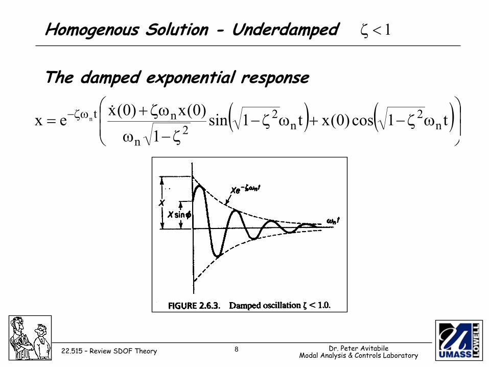
8 Dr. Peter AvitabileModal Analysis & Controls Laboratory22.515 – Review SDOF Theory
The damped exponential response
( ) ( )
ωζ−+ωζ−
ζ−ω
ζω+= ζω− t1cos)0(xt1sin
1)0(x)0(xex n
2n
22
n
ntn &
Homogenous Solution - Underdamped 1<ζ
9 Dr. Peter AvitabileModal Analysis & Controls Laboratory22.515 – Review SDOF Theory
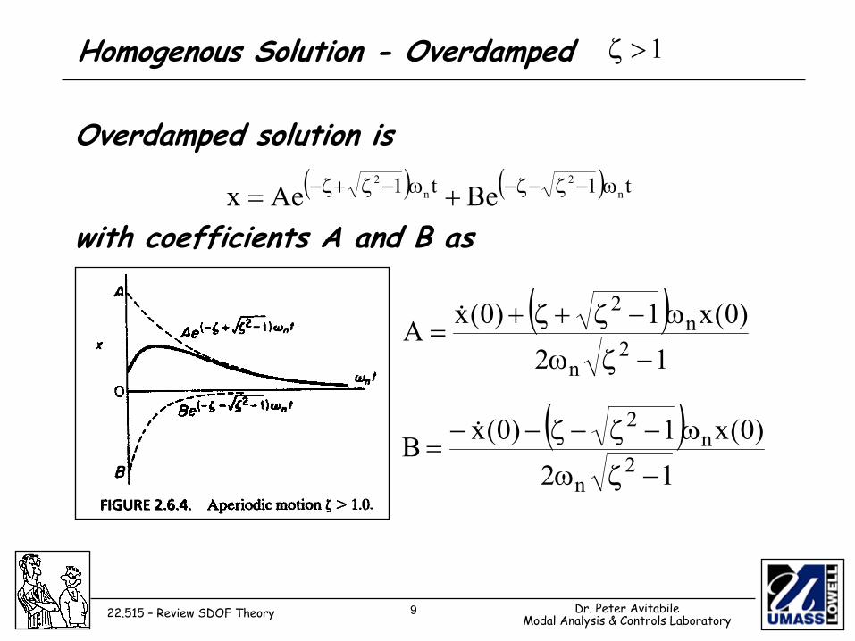
Overdamped solution is
with coefficients A and B as
Homogenous Solution - Overdamped 1>ζ
( ) ( ) t1t1 n2
n2
BeAex ω−ζ−ζ−ω−ζ+ζ− +=
( )12
)0(x1)0(xA2
n
n2
−ζω
ω−ζ+ζ+= &
( )12
)0(x1)0(xB2
n
n2
−ζω
ω−ζ−ζ−−= &
10 Dr. Peter AvitabileModal Analysis & Controls Laboratory22.515 – Review SDOF Theory
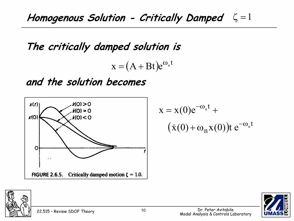
The critically damped solution is
and the solution becomes
Homogenous Solution - Critically Damped 1=ζ
( ) tneBtAx ω+=
( ) tn
t
n
n
et)0(x)0(x
e)0(xxω−
ω−
ω+
+=
&
11 Dr. Peter AvitabileModal Analysis & Controls Laboratory22.515 – Review SDOF Theory
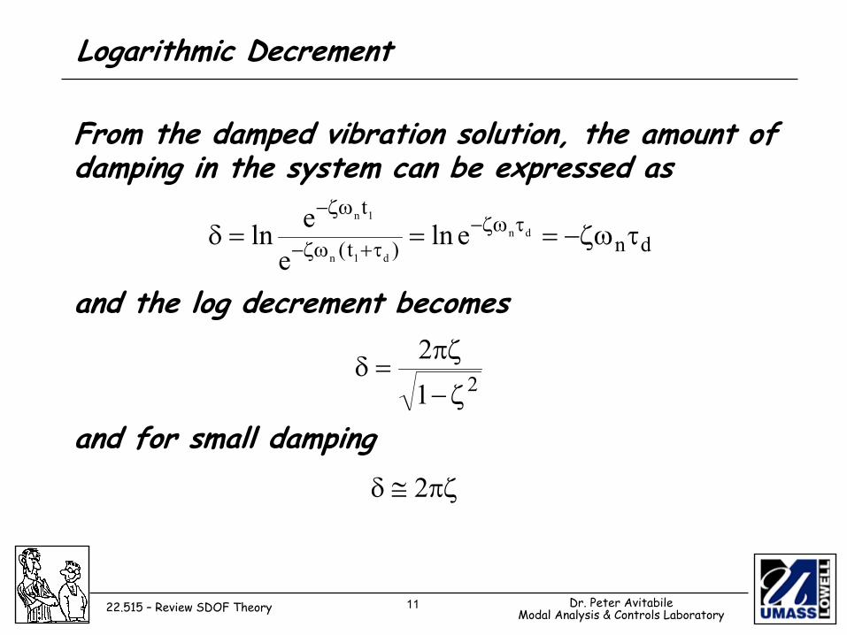
Logarithmic Decrement
From the damped vibration solution, the amount of damping in the system can be expressed as
and the log decrement becomes
and for small damping
dn)t(
tdn
d1n
1n
elneeln τζω−===δ τζω−
τ+ζω−
ζω−
212
ζ−
πζ=δ
πζ≅δ 2
12 Dr. Peter AvitabileModal Analysis & Controls Laboratory22.515 – Review SDOF Theory
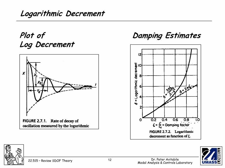
Logarithmic Decrement
Plot of Damping Estimates Log Decrement
13 Dr. Peter AvitabileModal Analysis & Controls Laboratory22.515 – Review SDOF Theory
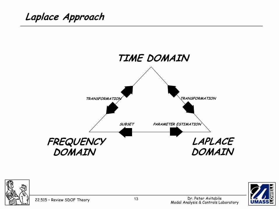
Laplace Approach
TIME DOMAIN
FREQUENCY
DOMAIN
LAPLACE
DOMAIN
TRANSFORMATION TRANSFORMATION
PARAMETER ESTIMATION SUBSET
14 Dr. Peter AvitabileModal Analysis & Controls Laboratory22.515 – Review SDOF Theory
Review - SDOF Definitions
• lumped mass• stiffness proportional to displacement
• damping proportional to velocity
• linear time invariant• 2nd order differential equations
Assumptions
m
k c
x(t) f(t)
15 Dr. Peter AvitabileModal Analysis & Controls Laboratory22.515 – Review SDOF Theory
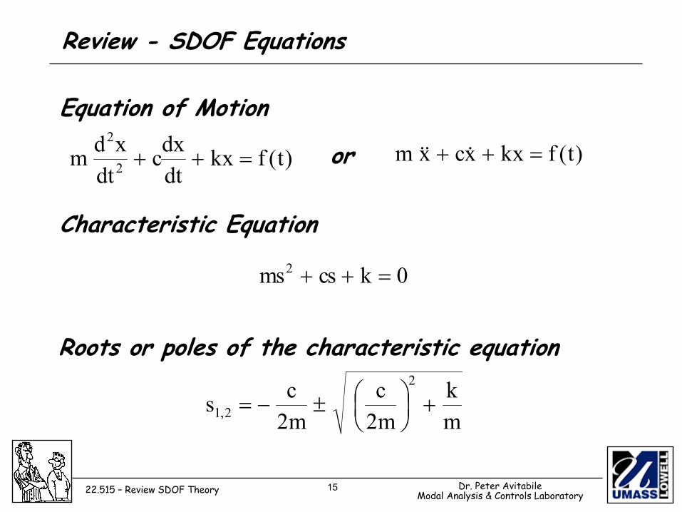
Review - SDOF Equations
Equation of Motion
)t(fxkdtdxc
dtxdm 2
2
=++ )t(fxkxcxm =++ &&&
Characteristic Equation
Roots or poles of the characteristic equation
0kscsm 2 =++
mk
m2c
m2cs
2
2,1 +
±−=
or
16 Dr. Peter AvitabileModal Analysis & Controls Laboratory22.515 – Review SDOF Theory
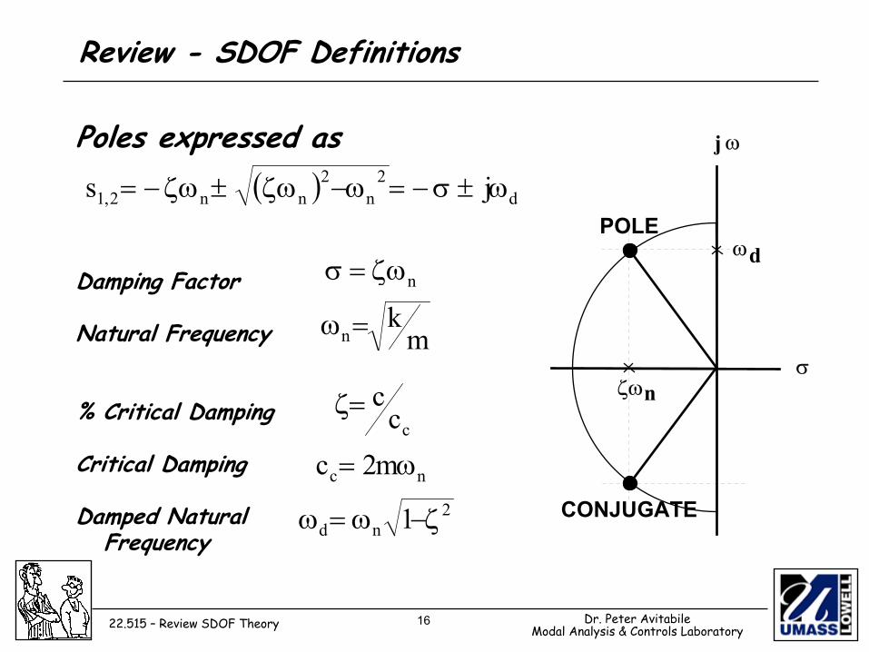
Review - SDOF Definitions
Poles expressed as
Damping Factor
Natural Frequency
% Critical Damping
Critical Damping
Damped NaturalFrequency
POLE
CONJUGATE
jω
σζωn
ωd
( ) d2n
2nn2,1 js ω±σ−=ω−ζω±ζω−=
nζω=σ
mk
n=ω
ccc=ζ
nc m2c ω=2
nd 1 ζ−ω=ω
17 Dr. Peter AvitabileModal Analysis & Controls Laboratory22.515 – Review SDOF Theory
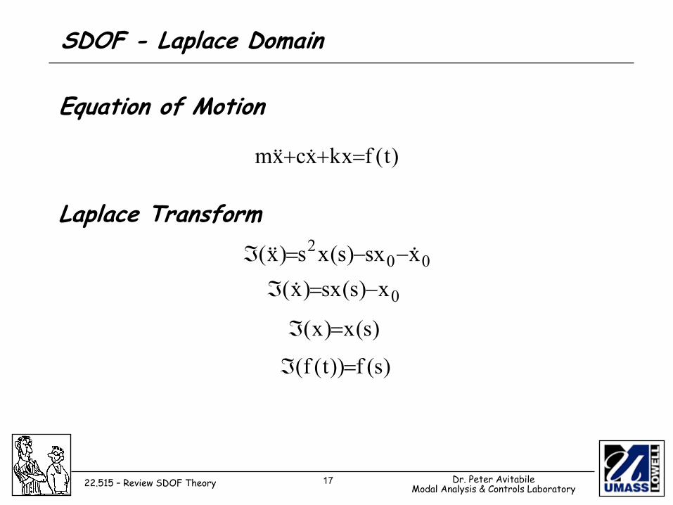
SDOF - Laplace Domain
Equation of Motion
Laplace Transform
)t(fxkxcxm =++ &&&
002 xxs)s(xs)x( &&& −−=ℑ
0x)s(xs)x( −=ℑ &
)s(x)x( =ℑ
)s(f))t(f( =ℑ
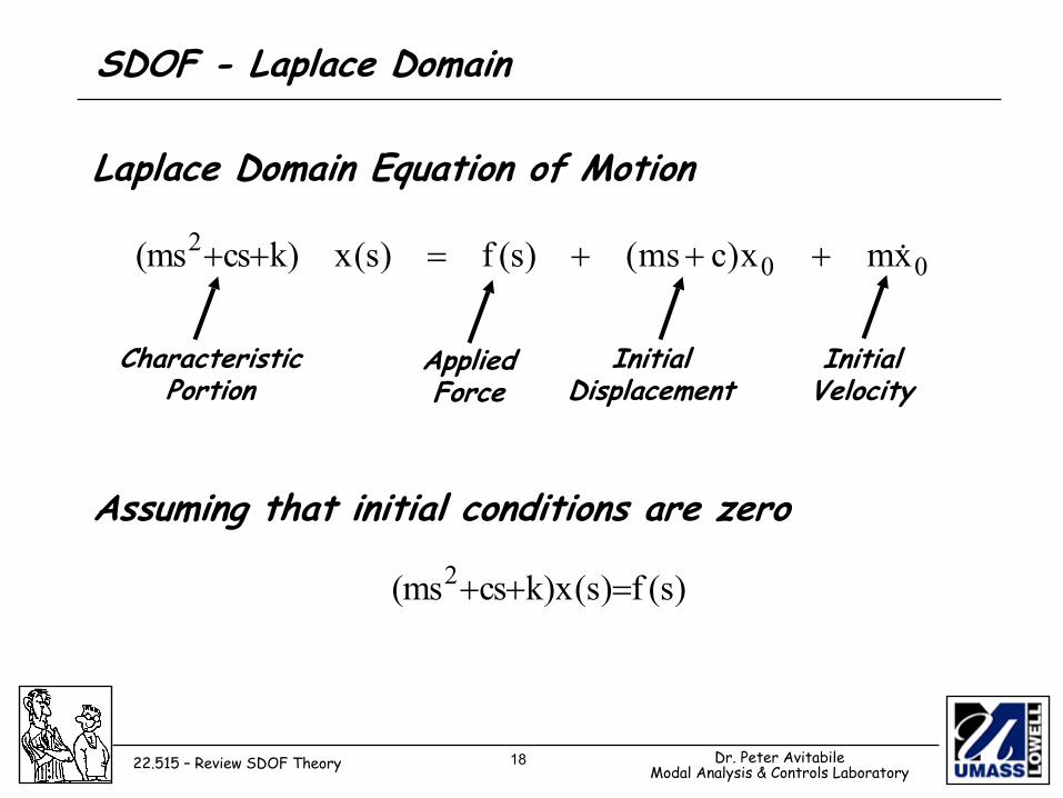
18 Dr. Peter AvitabileModal Analysis & Controls Laboratory22.515 – Review SDOF Theory
SDOF - Laplace Domain
Laplace Domain Equation of Motion
Assuming that initial conditions are zero
)s(f)s(x)kscsm( 2 =++
002 xmx)cms()s(f)s(x)kscsm( &+++=++
CharacteristicPortion
AppliedForce
InitialDisplacement
InitialVelocity
19 Dr. Peter AvitabileModal Analysis & Controls Laboratory22.515 – Review SDOF Theory
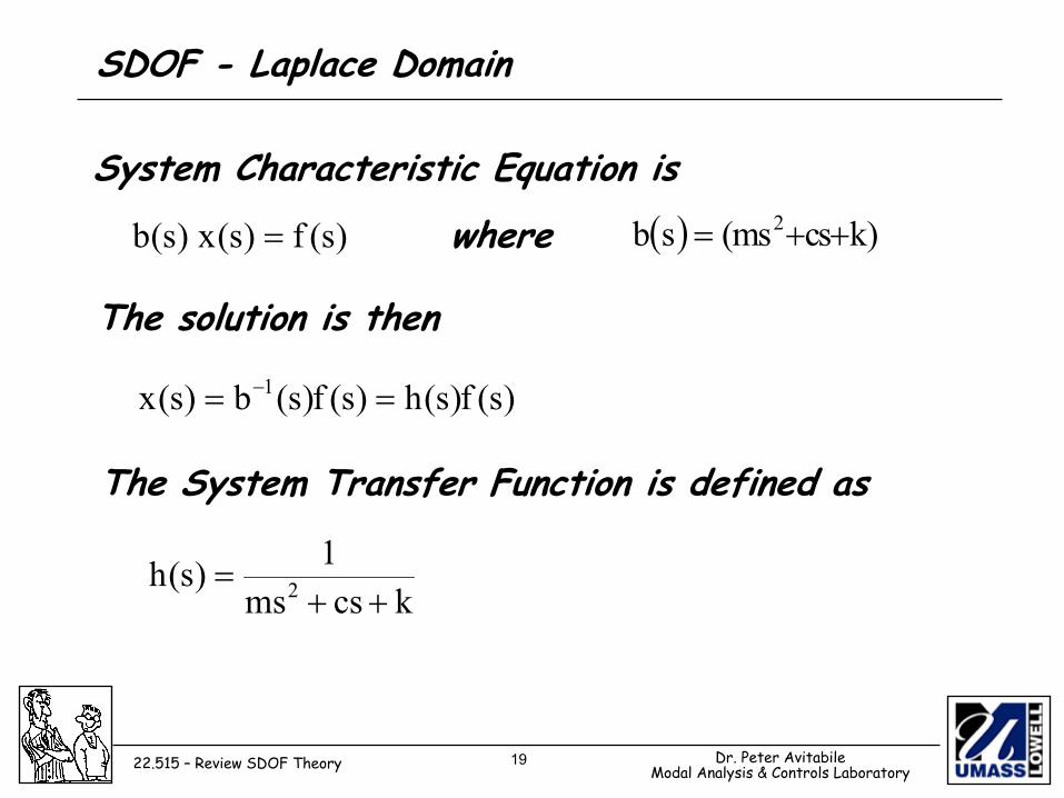
SDOF - Laplace Domain
System Characteristic Equation is
The solution is then
( ) )kscsm(sb 2 ++=where)s(f)s(x)s(b =
)s(f)s(h)s(f)s(b)s(x 1 == −
The System Transfer Function is defined as
kcsms1)s(h 2 ++
=
20 Dr. Peter AvitabileModal Analysis & Controls Laboratory22.515 – Review SDOF Theory
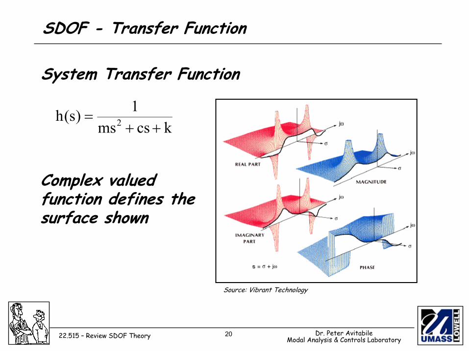
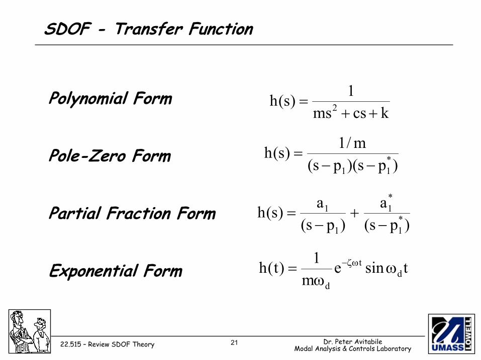
SDOF - Transfer Function
System Transfer Function
kcsms1)s(h 2 ++
=
Complex valued function defines the surface shown
Source: Vibrant Technology
21 Dr. Peter AvitabileModal Analysis & Controls Laboratory22.515 – Review SDOF Theory
SDOF - Transfer Function
Polynomial Form
Pole-Zero Form
Partial Fraction Form
Exponential Form
kcsms1)s(h 2 ++
=
)ps)(ps(m/1)s(h *
11 −−=
)ps(a
)ps(a)s(h *
1
*1
1
1
−+
−=
tsinem1)t(h d
t
d
ωω
= ζω−
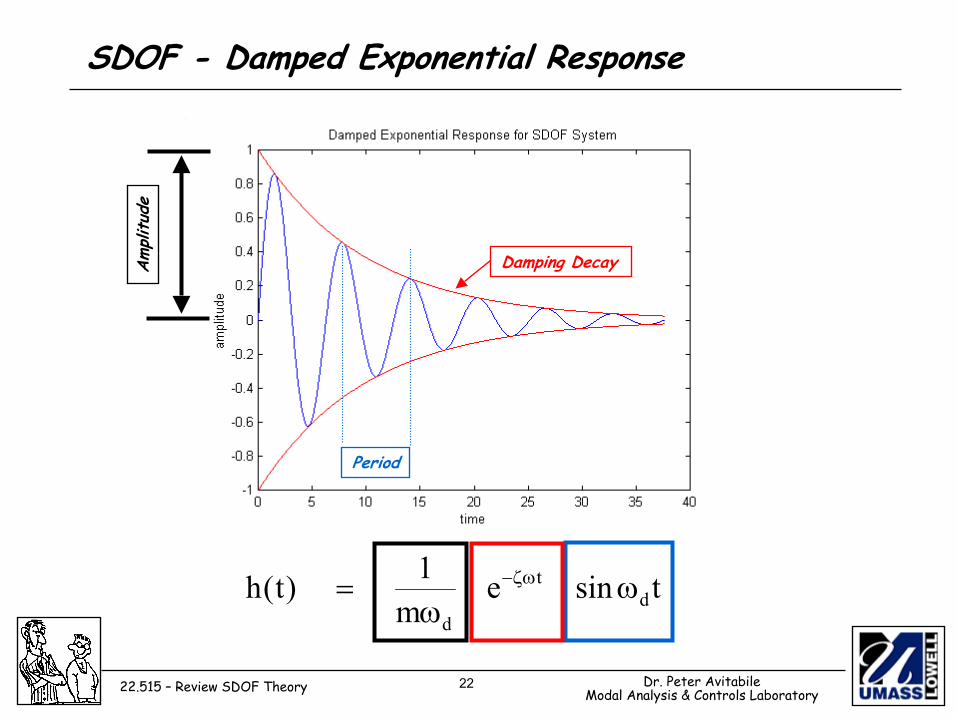
22 Dr. Peter AvitabileModal Analysis & Controls Laboratory22.515 – Review SDOF Theory
SDOF - Damped Exponential Response
tsinem1)t(h d
t
d
ωω
= ζω−
Amplitud
e
Damping Decay
Period
23 Dr. Peter AvitabileModal Analysis & Controls Laboratory22.515 – Review SDOF Theory
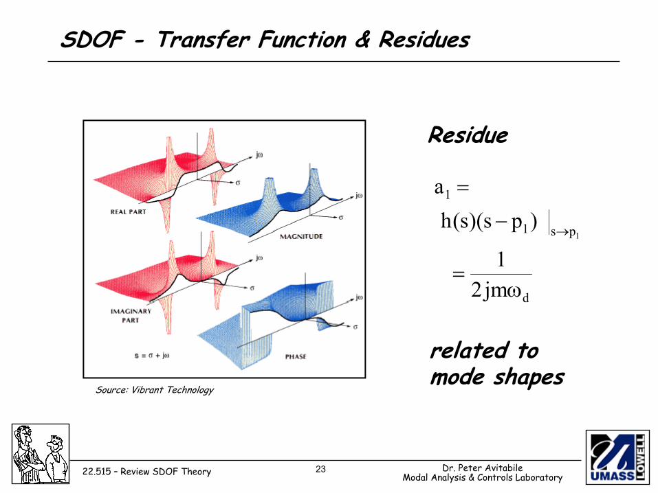
SDOF - Transfer Function & Residues
Residue
d
ps1
1
jm21
)ps)(s(ha
1
ω=
−
=
→
related to mode shapes
Source: Vibrant Technology
24 Dr. Peter AvitabileModal Analysis & Controls Laboratory22.515 – Review SDOF Theory
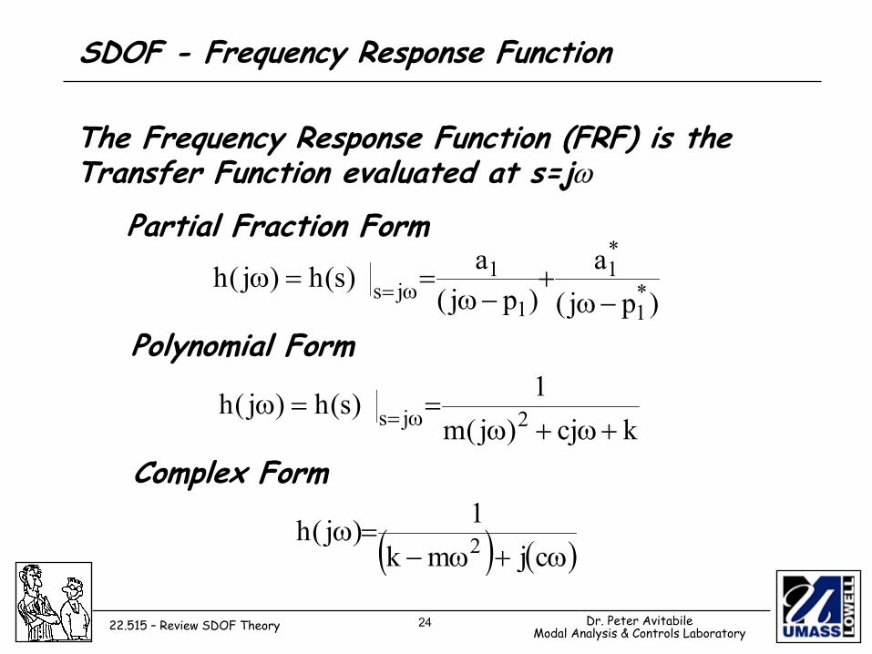
SDOF - Frequency Response Function
The Frequency Response Function (FRF) is the Transfer Function evaluated at s=jω
Partial Fraction Form
)pj(a
)pj(a)s(h)j(h *
1
*1
1
1js −ω
+−ω
==ω ω=
kcj)j(m1)s(h)j(h 2js +ω+ω
==ω ω=
Polynomial Form
( ) ( )ω+ω−=ω
cjmk1)j(h 2
Complex Form
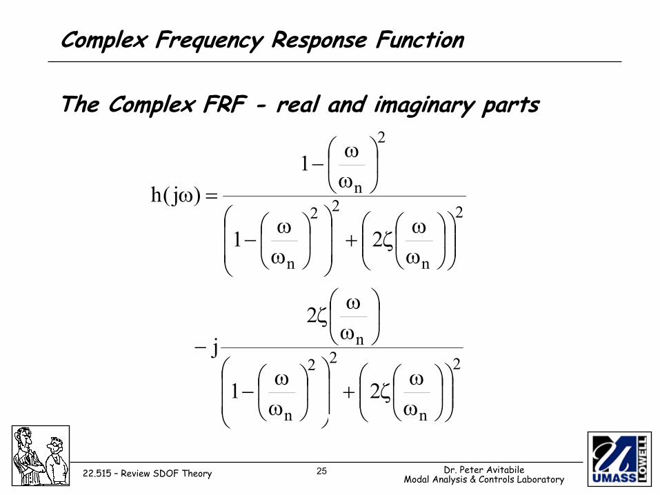
25 Dr. Peter AvitabileModal Analysis & Controls Laboratory22.515 – Review SDOF Theory
Complex Frequency Response Function
The Complex FRF - real and imaginary parts
2
n
22
n
n
2
n
22
n
2
n
21
2j
21
1)j(h
ωω
ζ+
ωω
−
ωω
ζ−
ωω
ζ+
ωω
−
ωω
−=ω
26 Dr. Peter AvitabileModal Analysis & Controls Laboratory22.515 – Review SDOF Theory
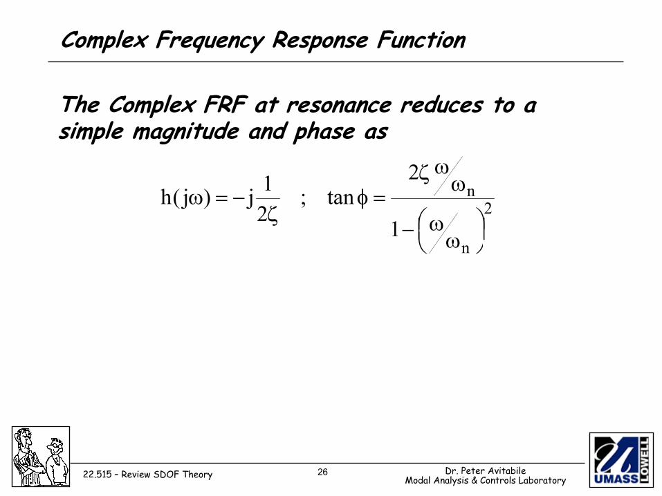
Complex Frequency Response Function
The Complex FRF at resonance reduces to a simple magnitude and phase as
2
n
n
1
2tan;
21j)j(h
ωω−
ωωζ
=φζ
−=ω
27 Dr. Peter AvitabileModal Analysis & Controls Laboratory22.515 – Review SDOF Theory
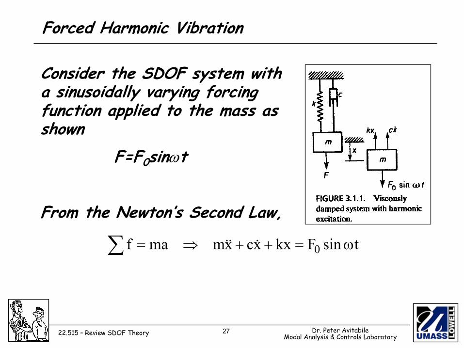
Forced Harmonic Vibration
Consider the SDOF system with a sinusoidally varying forcing function applied to the mass as shown
F=F0sinωt
From the Newton’s Second Law,
∑ ω=++⇒= tsinFkxxcxmmaf 0&&&

28 Dr. Peter AvitabileModal Analysis & Controls Laboratory22.515 – Review SDOF Theory
Forced Harmonic Vibration
The solution consists of the complementary solution (homogeneous solution) and the particular solution. The complementary part of the solution has already been discussed.The particular solution in the one of interest here. Since the oscillation of the response is at the same frequency as the excitation, the particular solution will be of the form
( )φ−ω= tsinXx
29 Dr. Peter AvitabileModal Analysis & Controls Laboratory22.515 – Review SDOF Theory
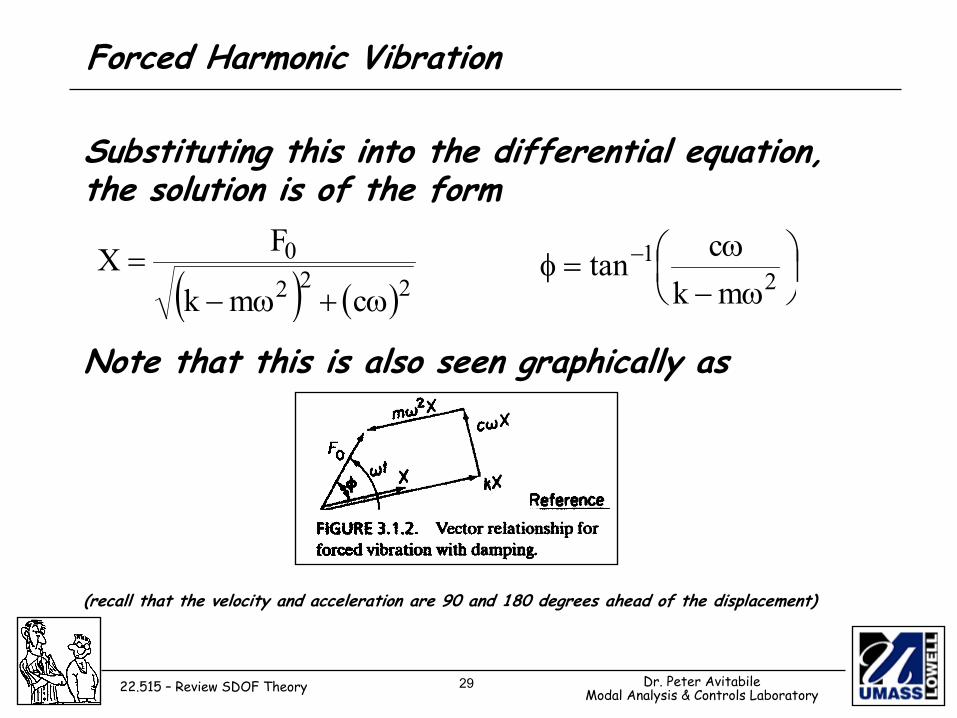
Forced Harmonic Vibration
Substituting this into the differential equation, the solution is of the form
Note that this is also seen graphically as
(recall that the velocity and acceleration are 90 and 180 degrees ahead of the displacement)
( ) ( )2220
cmk
FXω+ω−
=
ω−ω
=φ −2
1
mkctan
30 Dr. Peter AvitabileModal Analysis & Controls Laboratory22.515 – Review SDOF Theory
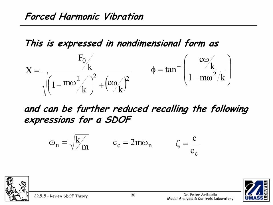
Forced Harmonic Vibration
This is expressed in nondimensional form as
and can be further reduced recalling the following expressions for a SDOF
( )222
0
kc
km1
kF
Xω+
ω−
=
ω−
ω=φ −
km1k
ctan 2
1
mk
n =ω nc m2c ω=ccc
=ζ
31 Dr. Peter AvitabileModal Analysis & Controls Laboratory22.515 – Review SDOF Theory
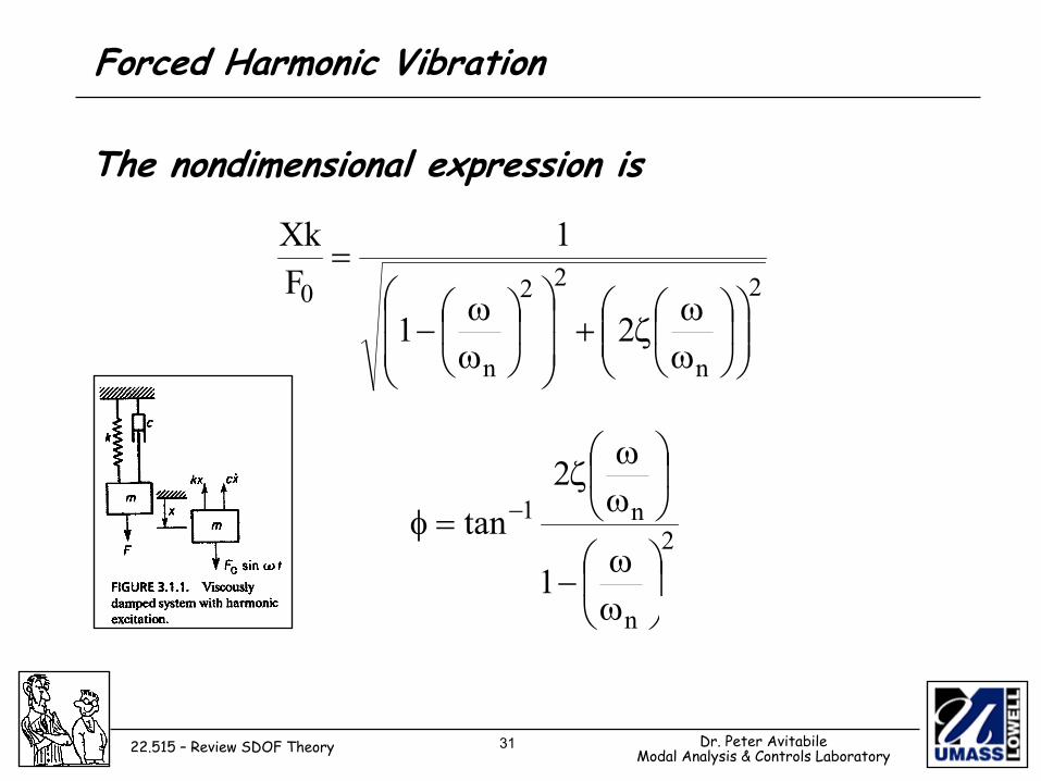
Forced Harmonic Vibration
The nondimensional expression is
2
n
22
n
021
1FXk
ωωζ+
ωω−
=
2
n
n1
1
2tan
ωω
−
ωω
ζ=φ −
32 Dr. Peter AvitabileModal Analysis & Controls Laboratory22.515 – Review SDOF Theory
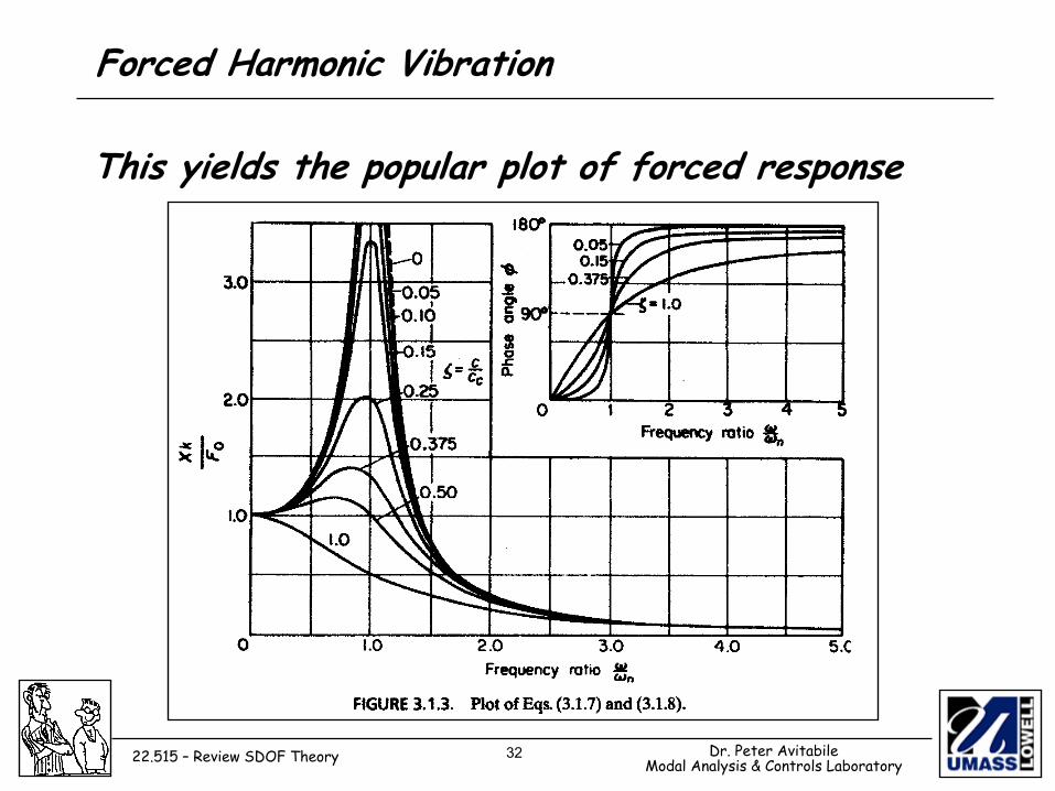
Forced Harmonic Vibration
This yields the popular plot of forced response
33 Dr. Peter AvitabileModal Analysis & Controls Laboratory22.515 – Review SDOF Theory
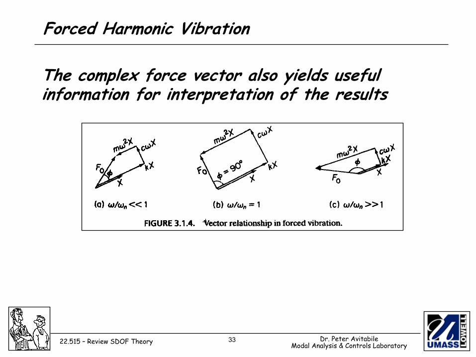
Forced Harmonic Vibration
The complex force vector also yields useful information for interpretation of the results
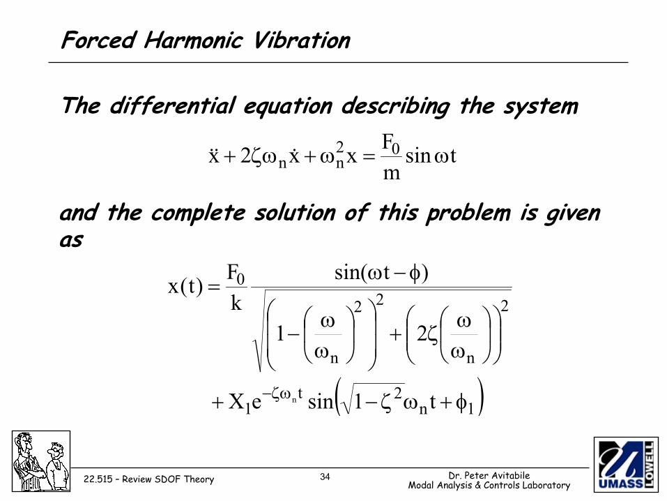
34 Dr. Peter AvitabileModal Analysis & Controls Laboratory22.515 – Review SDOF Theory
Forced Harmonic Vibration
The differential equation describing the system
and the complete solution of this problem is given as
tsinmFxx2x 02
nn ω=ω+ζω+ &&&
( )1n2t
1
2
n
22
n
0
t1sineX
21
)tsin(kF)t(x
n φ+ωζ−+
ωω
ζ+
ωω
−
φ−ω=
ζω−