Script for the Excel-based applet „StressTensor_v2.6.xls“ Heijn van Gent, MSc & Max Arndt, 06.07.2007

Aim of the applet: The aim of this applet is to calculate the stress (the total, normal and shear stress) on 18 planes, given a plane and a stress tensor, as well as establishing the magnitude and orientation of the principle stresses (and their ratio φ) of the same stress tensor. It also calculates whether these planes would fail, given two sets of material properties (for example, intact rock and healed faults, to calculate the possibility of faulting or reactivation). All data is combined in a Mohr diagram. In the sheet “Calculate own stress tensor!” you can input the (relative) size of the principle stresses, as well as the orientation of two stresses to calculate your own stress tensor (with one stress axes being vertical).

Input: The input of this applet consists of 18 planes (dip direction and dip angle), the six independent values of the symmetric stress tensor, and the cohesion, angle of internal friction and tensile strength of two materials.

Output: The output consist of the stress vector on the 18 planes, as well as the normal and shear stress components of this vector and the angles between the stress vector and the normal and shear components of this vector. Also the orientation of the three principle stresses (σ1-3), their ratio (Ф) is given. The Applet also calculates whether the plane would fail according to one or both of the given material properties and indicates this, both in text, as well as in a Schmidt Nett. Furthermore, a grid search is preformed, Here over 1500 pole points, using a 5° grid spacing, are tested for their failure potential, given the material properties and stress tensor. This way an overview is given of which orientations a plane needs to have to fail.

Coordinates systems: Different coordinate systems are used for the input, calculation and projection of the objects and angles in this applet. Input data is in the Polar coordinate system, with Azimuth and Plunge as the components. The Azimuth is the angle in degrees from the North line, which in this applet is defined as straight up in the diagrams. The Plunge is the deviation in degrees from the horizontal. Note that when planes are concerned, the Azimuth describes the Dip Direction and the Plunge equals the Dip of the plane. For the calculations, the right-handed 3D Cartesian vector coordinate system is used, where the following rules apply; the vectors have three elements, (x,y,z), the Cartesian axis are orthogonal and the x direction is up (north), y is right (east) and z is down. For the projection of the objects, a different, 2D Cartesian coordinate system is used, where x is right (east) and y is up (north).

Note to Excel In Excel, all angles are calculated as radian, while the output of the applet and in this script the angle will be described in degrees. Note that radians can be turned into degrees by dividing the radian value by (π/180).

Turning lineation and planes orientations into vectors: Being a line, a lineation can be transformed into a vector relatively easy. The vector is calculated using the formulas:

(1.1)

cos coscos sinsin

ϕ αϕ αϕ

= ⋅= ⋅=

xyz

Where α is the azimuth in degrees, and φ is the plunge, in °. A prerequisite of in this step is that the azimuth and plunge represent a line of the length 1. That means that the Cos (Plunge) represents the projection of the line on the xy-plane. In this applet, planes are initially characterized by their pole (a line (vector) perpendicular to the plane). The pole of a plane is calculated using the formulas:

Pole azimuth = Plane azimuth +180 Pole Dip = 90 – Plane dip

This line can then be turned into a vector using formulas (1.1). Note that since all vectors are recalculated into unit vectors (vectors with magnitude 1) before they are used further in this applet.

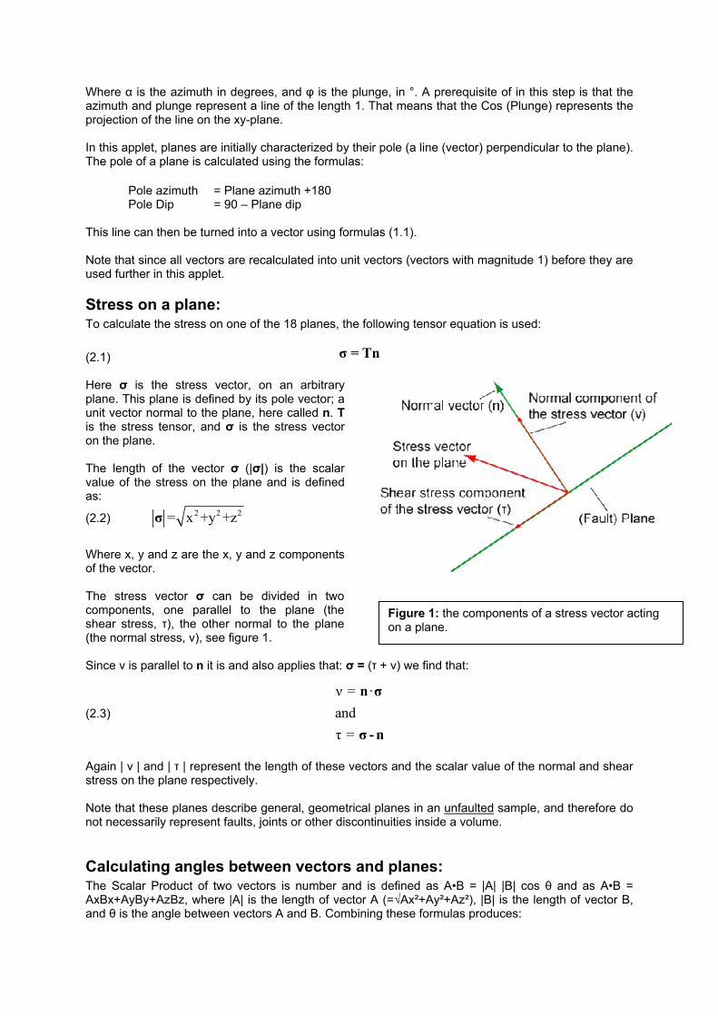
Stress on a plane: To calculate the stress on one of the 18 planes, the following tensor equation is used: (2.1) σ = Tn Here σ is the stress vector, on an arbitrary plane. This plane is defined by its pole vector; a unit vector normal to the plane, here called n. T is the stress tensor, and σ is the stress vector on the plane. The length of the vector σ (|σ|) is the scalar value of the stress on the plane and is defined as:

(2.2) 2 2 2= x +y +zσ

Where x, y and z are the x, y and z components of the vector. The stress vector σ can be divided in two components, one parallel to the plane (the shear stress, τ), the other normal to the plane (the normal stress, ν), see figure 1. Since ν is parallel to n it is and also applies that: σ = (τ + ν) we find that:

(2.3)

ν = ·andτ =

n σ

σ - n

Again | ν | and | τ | represent the length of these vectors and the scalar value of the normal and shear stress on the plane respectively. Note that these planes describe general, geometrical planes in an unfaulted sample, and therefore do not necessarily represent faults, joints or other discontinuities inside a volume.

Calculating angles between vectors and planes: The Scalar Product of two vectors is number and is defined as A•B = |A| |B| cos θ and as A•B = AxBx+AyBy+AzBz, where |A| is the length of vector A (=√Ax²+Ay²+Az²), |B| is the length of vector B, and θ is the angle between vectors A and B. Combining these formulas produces:

Figure 1: the components of a stress vector acting on a plane.

(2.4)

( )( )

1

1

2 2 2 2 2 2

·cos

cos

θ

θ

−

−

⎛ ⎞= ⎜ ⎟⎜ ⎟

⎝ ⎠⎛ ⎞

+ +⎜ ⎟= ⎜ ⎟⎜ ⎟⎝ ⎠

x x y y z z

x y z x y z

A BA B

A B A B A B

A A A B B B

Using this formula, the calculation of the angle between all lines is possible. Of course the angle between the shear and normal stress is per definition 90°. For the calculation of the angle between two planes, the same formula can be used, but the poles to the plane needs to bee used as input vector. The angle between two poles is the same as the angle between two planes. For the calculation of the angle between a line and a plane, the pole vector needs to bee used as input for the plane. Since the pole vector by definition has an angle of 90° to the plane, the angle between a line and a plane (θ’) is defined as θ’= 90 – θ.

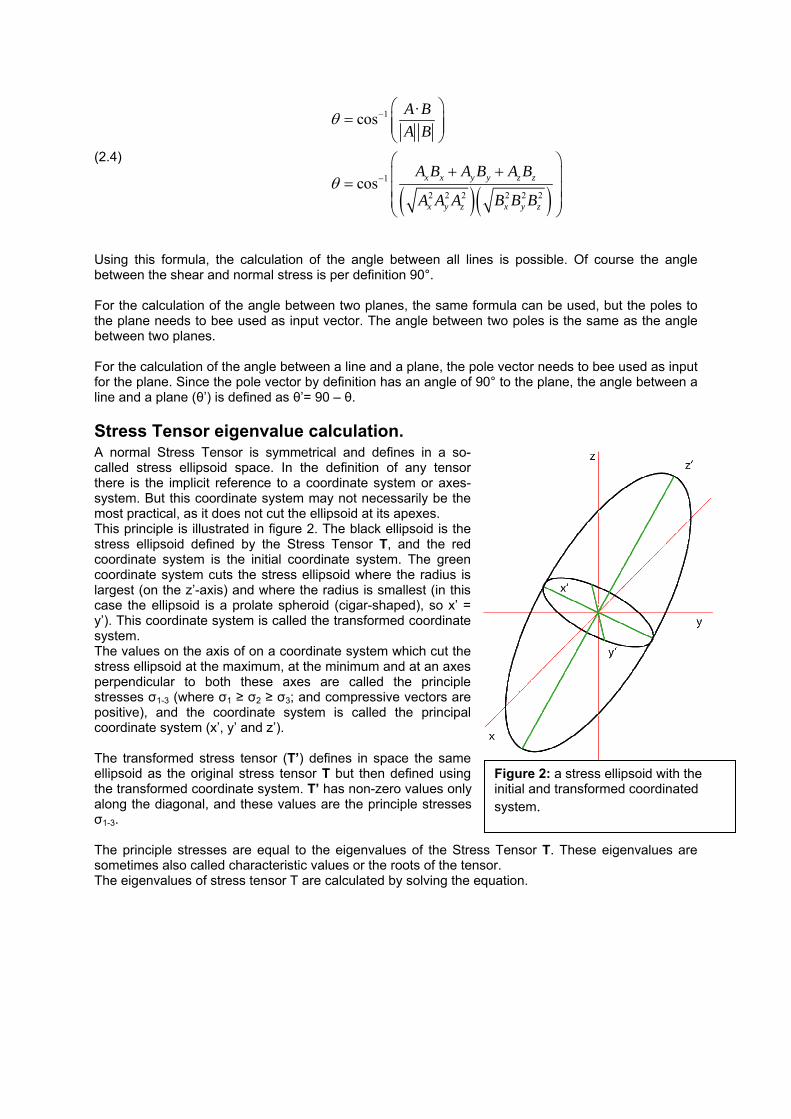
Stress Tensor eigenvalue calculation. A normal Stress Tensor is symmetrical and defines in a so-called stress ellipsoid space. In the definition of any tensor there is the implicit reference to a coordinate system or axes-system. But this coordinate system may not necessarily be the most practical, as it does not cut the ellipsoid at its apexes. This principle is illustrated in figure 2. The black ellipsoid is the stress ellipsoid defined by the Stress Tensor T, and the red coordinate system is the initial coordinate system. The green coordinate system cuts the stress ellipsoid where the radius is largest (on the z’-axis) and where the radius is smallest (in this case the ellipsoid is a prolate spheroid (cigar-shaped), so x’ = y’). This coordinate system is called the transformed coordinate system. The values on the axis of on a coordinate system which cut the stress ellipsoid at the maximum, at the minimum and at an axes perpendicular to both these axes are called the principle stresses σ1-3 (where σ1 ≥ σ2 ≥ σ3; and compressive vectors are positive), and the coordinate system is called the principal coordinate system (x’, y’ and z’). The transformed stress tensor (T’) defines in space the same ellipsoid as the original stress tensor T but then defined using the transformed coordinate system. T’ has non-zero values only along the diagonal, and these values are the principle stresses σ1-3. The principle stresses are equal to the eigenvalues of the Stress Tensor T. These eigenvalues are sometimes also called characteristic values or the roots of the tensor. The eigenvalues of stress tensor T are calculated by solving the equation.

Figure 2: a stress ellipsoid with the initial and transformed coordinated system.

(2.5)

µa b cd e f µg h i

a b c µ 0d e f µ 0g h i µ 0

a-µ b cd e-µ f 0g h i-µ

⎡ ⎤ ⎡ ⎤ ⎡ ⎤⎢ ⎥ ⎢ ⎥ ⎢ ⎥=⎢ ⎥ ⎢ ⎥ ⎢ ⎥⎢ ⎥ ⎢ ⎥ ⎢ ⎥⎣ ⎦ ⎣ ⎦ ⎣ ⎦

⎡ ⎤ ⎡ ⎤ ⎡ ⎤ ⎡ ⎤⎢ ⎥ ⎢ ⎥ ⎢ ⎥ ⎢ ⎥− =⎢ ⎥ ⎢ ⎥ ⎢ ⎥ ⎢ ⎥⎢ ⎥ ⎢ ⎥ ⎢ ⎥ ⎢ ⎥⎣ ⎦ ⎣ ⎦ ⎣ ⎦ ⎣ ⎦

=

x xy yz z

x xy yz z

TX = X

Here T is the stress tensor, X is a vector and µ is a constant (this equation describes a vector X which direction does not change when the deformation T is applied to it, but it length changes with a factor µ). The last line in equation 2.5 shows that µ can be solved by solving det(T-µI)=0 (I is the identity matrix). Note that a-i are the known components of T. det(T-µI)=0 is solved like:

(2.6)

( ) ( )( )3 2

3 2

a-µ b cd e-µ f =0g h i-µ

e-µ f b c b ca-µ -d +g =0

h i-µ h i-µ e-µ f

a-µ e-µ * i-µ -h*f -d(b*(i-µ)-h*c)+g(b*f-(e-µ)-c)=0

-µ +(i+a+e)µ +(-a*i-e*i-a*e+c*g+f*h+b*d)µ+(a*e*i+b*f*g+c*d*h-c*g*e-f*h*a-b*d*i)=0µ -(i+a+e)µ -(-a*i-e*i-a*e+

3 22 1 0

c*g+f*h+b*d)µ-(a*e*i+b*f*g+c*d*h-c*g*e-f*h*a-b*d*i)=0µ +(a )µ +(a )µ+(a )=0

The last line in equation 2.6 can be solved using the Cubic formula (similar to the quadratic or ABC-formula for solving quadratic equations). The three real solutions of the Cubic formula then equal the eigen values and are (from mathworld.wolfram.com/CubicFormula.html):

(2.7)

2

2

2

-1

3

21 2

32 1 0 2

θ 1z1=2 -Qcos - a3 3

θ+2π 1z2=2 -Qcos - a3 3

θ+4π 1z3=2 -Qcos - a3 3

where

Rθ=cos-Q

3a -aQ=9

9(a a )-27a -2aR=54

⎛ ⎞⎜ ⎟⎝ ⎠

⎛ ⎞⎜ ⎟⎝ ⎠⎛ ⎞⎜ ⎟⎝ ⎠

⎛ ⎞⎜ ⎟⎜ ⎟⎝ ⎠

There the largest value of z1, z2 and z3 is σ1 and the smallest value of z1, z2 and z3 equals σ3. Of course z2 equals σ2. The ratio defining the relation between σ1, σ2 and σ3, Ф, is defined as:

(2.8) ( )( )

2 3

1 3

σ -σΦ=

σ -σ

This ratio is often used in stress tensor calculation and stress tensor inversions to describe the shape of the principle stress tensor, because the absolute values of the Tensor can not be calculated.

Calculating the eigenvectors of the Stress Tensor The vectors defining the transformed coordinate system in the original coordinate can be found by solving the eigenvectors of the tensor T. For the different characteristic values (that is σ1, σ2 and σ3) the eigenvectors can be found by solving the sets of equations:

(2.9)

1 1 1 1

1 1 1 1 1

1 1 1 1

2 2 2 2

2 2 2 2 2

2 2 2 2

3 3 3 3

3 3 3 3 3

3 3 3 3

(a-σ )x +by +cz =0for σ : dx +(e-σ )y +fz =0

gx +hy +(i-σ )z =0

(a-σ )x +by +cz =0for σ : dx +(e-σ )y +fz =0

gx +hy +(i-σ )z =0

(a-σ )x +by +cz =0for σ : dx +(e-σ )y +fz =0

gx +hy +(i-σ )z =0

Here x, y and z define the eigenvectors for the appropriate characteristic values. Solving these sets of equations in Excel is complicated. Normally one would assume one value of xj, yj or zj (j = 1, 2 or 3) to be 1, and solve the set of equations to calculate the other two values. However it is possible that the selected value is 0, rendering the calculation useless. It is however possible to ascertain a priority whether xj, yj or zj is 0, using the sub determinants; if the sub determinant of xj, yj or zj is 0, then xj, yj or

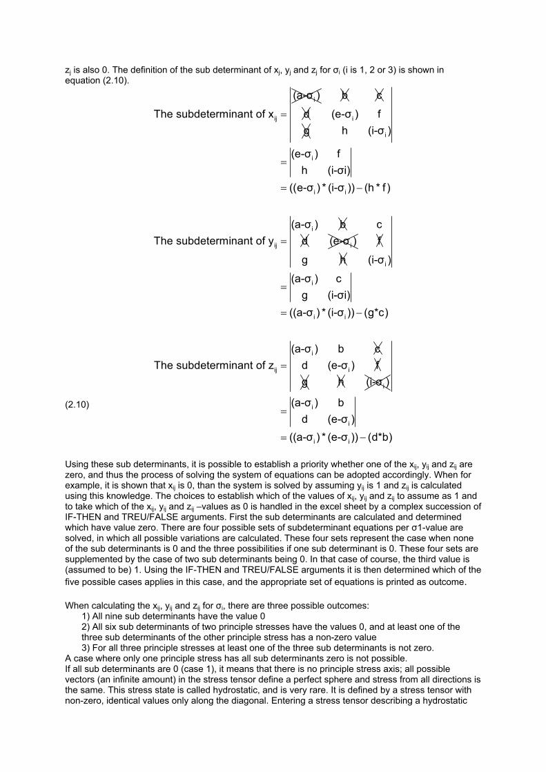
zj is also 0. The definition of the sub determinant of xj, yj and zj for σi (i is 1, 2 or 3) is shown in equation (2.10).

(2.10)

=i

ij

(a-σ )

The subdeterminant of x

b c

d i(e-σ ) fg

=

= −

=

i

i

i i

i

ij

h (i-σ )

(e-σ ) fh (i-σi)

((e-σ ) * (i-σ )) (h * f )

(a-σ ) bThe subdeterminant of y

cd i(e-σ ) f

g h

=

= −

=

i

i

i i

i

ij

(i-σ )

(a-σ ) cg (i-σi)

((a-σ ) * (i-σ )) (g*c)

(a-σ ) b cThe subdeterminant of z id (e-σ ) f

g h i(i-σ )

=

= −

i

i

i i

(a-σ ) bd (e-σ )

((a-σ ) * (e-σ )) (d*b)

Using these sub determinants, it is possible to establish a priority whether one of the xij, yij and zij are zero, and thus the process of solving the system of equations can be adopted accordingly. When for example, it is shown that xij is 0, than the system is solved by assuming yij is 1 and zij is calculated using this knowledge. The choices to establish which of the values of xij, yij and zij to assume as 1 and to take which of the xij, yij and zij –values as 0 is handled in the excel sheet by a complex succession of IF-THEN and TREU/FALSE arguments. First the sub determinants are calculated and determined which have value zero. There are four possible sets of subdeterminant equations per σ1-value are solved, in which all possible variations are calculated. These four sets represent the case when none of the sub determinants is 0 and the three possibilities if one sub determinant is 0. These four sets are supplemented by the case of two sub determinants being 0. In that case of course, the third value is (assumed to be) 1. Using the IF-THEN and TREU/FALSE arguments it is then determined which of the five possible cases applies in this case, and the appropriate set of equations is printed as outcome. When calculating the xij, yij and zij for σi, there are three possible outcomes:

1) All nine sub determinants have the value 0 2) All six sub determinants of two principle stresses have the values 0, and at least one of the three sub determinants of the other principle stress has a non-zero value 3) For all three principle stresses at least one of the three sub determinants is not zero.

A case where only one principle stress has all sub determinants zero is not possible. If all sub determinants are 0 (case 1), it means that there is no principle stress axis; all possible vectors (an infinite amount) in the stress tensor define a perfect sphere and stress from all directions is the same. This stress state is called hydrostatic, and is very rare. It is defined by a stress tensor with non-zero, identical values only along the diagonal. Entering a stress tensor describing a hydrostatic

stress state will not result in a successful calculation, as this applet is designed to calculate shear stresses, and a hydrostatic stress state is defined by its lack of shear stresses. If all sub determinants of two principle stresses are 0 and at least one of the sub determinants is not-zero (case 2), it means that these two principle stresses have no fixed orientation. Together they describe a perfect circle in the stress ellipsoid, perpendicular to the orientation of the third principle value. In practice this means that the stress ellipsoid is a prolate ellipsoid, defining an uniaxial stress state. The principle values of the two undefined vectors are the same and an uniaxial matrix consist of no-zero vales only occurring along the diagonal, and two of these values are identical. In case 3 the stress tensor defines a triaxial state where all principle stresses can be determined and there are three principle stresses with different values. The case with only one principle stress with three sub determinants being 0 is not possible, as this would imply that the other two vectors are defined. Since the three principle stress vectors are at angles of 90° relative to each other, knowing two axes will automatically result in knowing the orientation of the third vector.

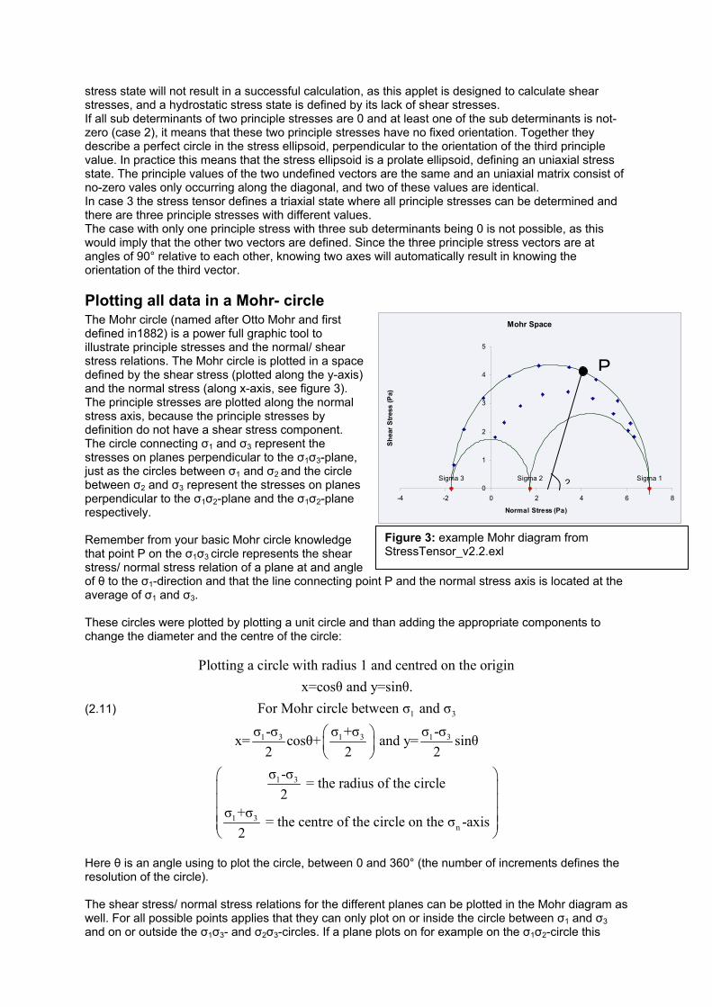
Plotting all data in a Mohr- circle The Mohr circle (named after Otto Mohr and first defined in1882) is a power full graphic tool to illustrate principle stresses and the normal/ shear stress relations. The Mohr circle is plotted in a space defined by the shear stress (plotted along the y-axis) and the normal stress (along x-axis, see figure 3). The principle stresses are plotted along the normal stress axis, because the principle stresses by definition do not have a shear stress component. The circle connecting σ1 and σ3 represent the stresses on planes perpendicular to the σ1σ3-plane, just as the circles between σ1 and σ2 and the circle between σ2 and σ3 represent the stresses on planes perpendicular to the σ1σ2-plane and the σ1σ2-plane respectively. Remember from your basic Mohr circle knowledge that point P on the σ1σ3 circle represents the shear stress/ normal stress relation of a plane at and angle of θ to the σ1-direction and that the line connecting point P and the normal stress axis is located at the average of σ1 and σ3. These circles were plotted by plotting a unit circle and than adding the appropriate components to change the diameter and the centre of the circle:

(2.11) 1 3

1 3 1 3 1 3

1 3

1 3

Plotting a circle with radius 1 and centred on the originx=cosθ and y=sinθ.

For Mohr circle between σ and σσ -σ σ +σ σ -σx= cosθ+ and y= sinθ

2 2 2σ -σ = the radius of the circle

2σ +σ = the cent

2

⎛ ⎞⎜ ⎟⎝ ⎠

nre of the circle on the σ -axis

⎛ ⎞⎜ ⎟⎜ ⎟⎜ ⎟⎜ ⎟⎝ ⎠

Here θ is an angle using to plot the circle, between 0 and 360° (the number of increments defines the resolution of the circle). The shear stress/ normal stress relations for the different planes can be plotted in the Mohr diagram as well. For all possible points applies that they can only plot on or inside the circle between σ1 and σ3 and on or outside the σ1σ3- and σ2σ3-circles. If a plane plots on for example on the σ1σ2-circle this

Mohr Space

Sigma 1Sigma 3 Sigma 20

1

2

3

4

5

-4 -2 0 2 4 6 8

Normal Stress (Pa)

Shea

r Stre

ss (P

a)

2

P

Figure 3: example Mohr diagram from StressTensor_v2.2.exl

means that the pole of the plane lies within the plane defined by the σ1 σ2 vectors (i.e. the pole is perpendicular to the σ3-vector). Ergo planes that plot on the σ2σ3-circle, have a pole perpendicular to the σ1- vector and planes that plot between the circles have pole not perpendicular to any of the principle directions.

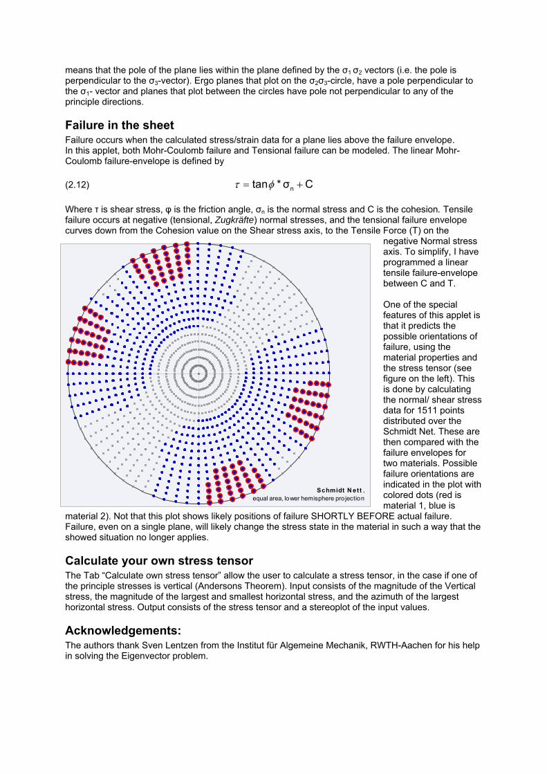
Failure in the sheet Failure occurs when the calculated stress/strain data for a plane lies above the failure envelope. In this applet, both Mohr-Coulomb failure and Tensional failure can be modeled. The linear Mohr- Coulomb failure-envelope is defined by (2.12) ntan *σ Cτ φ= + Where τ is shear stress, φ is the friction angle, σn is the normal stress and C is the cohesion. Tensile failure occurs at negative (tensional, Zugkräfte) normal stresses, and the tensional failure envelope curves down from the Cohesion value on the Shear stress axis, to the Tensile Force (T) on the

negative Normal stress axis. To simplify, I have programmed a linear tensile failure-envelope between C and T. One of the special features of this applet is that it predicts the possible orientations of failure, using the material properties and the stress tensor (see figure on the left). This is done by calculating the normal/ shear stress data for 1511 points distributed over the Schmidt Net. These are then compared with the failure envelopes for two materials. Possible failure orientations are indicated in the plot with colored dots (red is material 1, blue is

material 2). Not that this plot shows likely positions of failure SHORTLY BEFORE actual failure. Failure, even on a single plane, will likely change the stress state in the material in such a way that the showed situation no longer applies.

Calculate your own stress tensor The Tab “Calculate own stress tensor” allow the user to calculate a stress tensor, in the case if one of the principle stresses is vertical (Andersons Theorem). Input consists of the magnitude of the Vertical stress, the magnitude of the largest and smallest horizontal stress, and the azimuth of the largest horizontal stress. Output consists of the stress tensor and a stereoplot of the input values.

Acknowledgements: The authors thank Sven Lentzen from the Institut für Algemeine Mechanik, RWTH-Aachen for his help in solving the Eigenvector problem.

Schmidt N ett , equal area, lower hemisphere pro jection