SCHRÖDINGER’S TRAIN OF THOUGHT

SCHRÖDINGER’S TRAIN OF THOUGHTNicholas Wheeler, Reed College Physics Department

April 2006

Introduction. David Griffiths, in his Introduction to Quantum Mechanics (2nd

edition, 2005), is content—at equation (1.1) on page 1—to pull (a typicalinstance of) the Schrodinger equation

i� ∂Ψ∂t

= − �2

2m∂2Ψ∂x2

+ V Ψ

out of his hat, and then to proceed directly to book-length discussion of itsinterpretation and illustrative physical ramifications. I remarked when I wrotethat equation on the blackboard for the first time that in a course of my owndesign I would feel an obligation to try to encapsulate the train of thoughtthat led Schrodinger to his equation (1926), but that I was determined on thisoccasion to adhere rigorously to the text. Later, however, I was approached byseveral students who asked if I would consider interpolating an account of thehistorical events I had felt constrained to omit. That I attempt to do here. Itseems to me a story from which useful lessons can still be drawn.

1. Prior events. Schrodinger cultivated soil that had been prepared by others.Planck was led to write E = hν by his successful attempt (1900) to use thethen-recently-established principles of statistical mechanics to account for thespectral distribution of thermalized electromagnetic radiation. It was soonappreciated that Planck’s energy/frequency relation was relevant to theunderstanding of optical phenomena that take place far from thermalequilibrium (photoelectric effect: Einstein 1905; atomic radiation: Bohr 1913).By 1916 it had become clear to Einstein that, while light is in some contexts welldescribed as a Maxwellian wave, in other contexts it is more usefully thoughtof as a massless particle, with energy E = hν and momentum p = h/λ. Themechanical statement E = cp1 and the wave relation λν = c become thenalternative ways of saying the same thing. Einstein had in effect “invented thephoton” (which, however, did not acquire its name until 1926, when it wasbestowed by the American chemist, Gilbert Lewis).

In 1923, Louis de Broglie—then a thirty-one-year-old graduate student atthe University of Paris—speculated that if light waves are in some respects

1 This is the relativistic statement E = c√

p2 + (mc)2 in the limit m ↓ 0.

2 Schrodinger’s train of thought

particle-like, perhaps particles are in some respects wave-like, with frequencyand wavelength that stand in the relation (hν) = c

√(h/λ)2 + (mc)2.2 It was

obvious to others that if particles are indeed in some respects “wave-like” thenthey should exhibit the interference and diffractive effects most characteristicof waves. Electron diffraction was in fact observed by Davisson & Germer atBell Labs in 1927, but by then Schrodinger had already completed his work.

Schrodinger cannot have been the only one to appreciate that the wave-likeproperties of particles—if any—must be describable by a wave equation of somesort. Because de Broglie had been led to his idea by Einstein and relativity,so also—and for that reason—were Schrodinger’s initial efforts relativistic. Heobserved that if one looks for planewave solutions

ϕ(xxx, t) = exp{

i�[ppp···xxx − Et]

}of {

1c2

∂2

∂t2− ∂2

∂x2− ∂2

∂y2− ∂2

∂z2+ (mc/�)2

}ϕ = 0

one immediately recovers (E/c)2 = ppp···ppp + (mc)2, but when he attempted to usea modification of the preceding equation3 to compute the energy spectrum ofhydrogen he obtained results that were not in agreement with the measuredvalues.4

2 This is more neatly formulated ω = c√

k2 + κ2 , where ω = 2πν, k = 2π/λand κ = mc/�. De Broglie had written mc2 = hν and interpreted ν to referto some kind of “interior vibration.” He then set the particle into motionand observed that m increased while ν—owing to time dilation—decreased, sohad a sophomoric “paradox” on his hands. It was from an effort to resolve theparadox—not from mere idle word play—that his idea was born. For an Englishtranslation of his brief paper, visit http://www.davis-inc.com/physics/. At theend of his paper de Broglie remarked that if a mass pursues a circular orbitof radius r with momentum p, and if we can assume that Einstein’s p = h/λpertains not only to light quanta but also to particles, then Bohr’s quantizationof angular momentum rp = n� can be interpreted as the stipulation that thecircumference of the orbit be integrally many wavelengths long: 2πr = nλ.The architecture of the Bohr atom could thus be understood in a new way.This modest accomplishment notwithstanding, de Broglie’s advisors were sodubious that they sent the text of his work to Einstein for evaluation. Einstein,on the other hand, was so favorably impressed that he appended to a paper ofhis own—then in press—a note reporting that he had learned of an idea putforward by one Louis de Broglie that he thought merited closer study. It wasthis note that engaged Schrodinger’s attention.

3 It is known today as the Klein-Gordon equation, and is of fundamentalimportance in a connection distinct from the one originally contemplated bySchrodinger.

4 See L. I. Schiff, Quantum Mechanics (3rd edition 1968, page 470) for thedetails, which Schrodinger published in 1926 after his non-relativistic paperswere already in print.

Optical side of the analogy 3

So he put the work aside, not—so the story goes—to take it up againuntil Peter Debye asked him to present a seminar at the ETH (EidgenossischeTechnische Hochschule) in Zurich, to which they were both attached at thetime. For the occasion, Schrodinger chose to develop a non-relativistic versionof his earlier work. Schrodinger (1887–1961) was 38 in 1925, only eight yearsyounger than Einstein, five years younger than Born, two years younger thanBohr and—by a wide margin—the “old man” among the founding fathers of the“new quantum theory” (Pauli was 25, Heisenberg was 24, Dirac was 23). Partlyas a result of his unusually thorough and well-rounded formal education (hehad been a student of Fritz Hasenohrl, Boltzmann’s successor at the Universityof Vienna) and partly because of his prior research experience, Schrodinger’sknowledge of physics appears to have been in many respects much broaderthan that of his junior colleagues. This fact made it possible for Schrodingerto approach his objective with an erudite circumspection that was, I suspect,quite beyond their reach. Schrodinger was uniquely positioned to do what hedid.

Schrodinger remarked that optics came into the world as a theory of rays,which broadened into a wave theory from which ray optics could be recoveredas a certain (high-frequency) approximation, and that at the interface betweenthe two theories stood a certain elegant formalism (“theory of the characteristicfunction”) that had been devised by Hamilton—devised without reference towave theory—nearly a century earlier.5 Schrodinger was aware also thatHamilton himself had noticed (then forgotten, then noticed again) that it ispossible to construct a formalism (known today as Hamilton-Jacobi theory)that stands to the classical theory of particle trajectories as the theory ofcharacteristic functions stands to the classical theory of rays. Schrodingerproposed to complete the optico-mechanical analogy by constructing a “wavemechanics of particles” that stands to Hamilton-Jacobi theory (whence to thetheory of particle trajectories) as optical wave theory stands to characteristicfunction theory (whence to the theory of optical rays).

2. Review of the situation on the optical side of the analogy. For the purposes athand it serves to pretend that light is a scalar wave phenomenon, described invacuum by the simple wave equation

�2ϕ(xxx, t) = 1c2

∂2

∂t2ϕ(xxx, t) (1)

It is from the linearity of this equation (i.e., from the availability of a principleof superposition) that optical interference effects arise, in which connection

5 Hamilton’s ideas were developed in a pair of papers that were publishedunder the title “Theory of systems of rays” in 1830 and 1832. The central ideawas adapted to mechanics in “On a general method in dynamics” (1834). Bythe late 19th Century Hamilton-Jacobi methods were used routinely to studythe 3-body problem, the stability of the solar system and similar problems. Aparticipant in that work was H. Bruns, who in 1895 had the bright idea of usingthose methods to in effect reinvent Hamiltonian optics.


we recall that local field intensity is proportional to the square of local fieldstrength.

Separation of the time variable leads to the theory of monochromatic wavefields

ϕ(xxx, t) = f(xxx) · e−iωt with �2f(xxx) + k2f(xxx) = 0 : k2 ≡ (ω/c)2

Monochromatic planewaves are produced in cases of the type

f(xxx) ∼ eik nnn···xxx

Surfaces of constant phase are in such cases planes normal to the unit vectornnn, defined by equations of the form

nnn···xxx = constant

We then have

ϕ(xxx, t) ∼ ei[k nnn···xxx − ωt]

↓

∼ ei[kx − ωt] in the one-dimensional case

To compute—in the one-dimensional case—the speed with which points ofconstant phase advance we set d

dt [kx − ωt] = 0 and obtain v = ω/k = c. Inthe three-dimensional case we note that the advance is along the local normal,so write xxx = x nnn and are led back to the same result.

If the vacuum is replaced by the simplest kind of refractive medium weexpect the wave equation (1) to be replaced by

�2ϕ(xxx, t) =[n(xxx)

c

]2 ∂2

∂t2ϕ(xxx, t) (2)[n(xxx)

c

]= 1

v(xxx)

where n(xxx) refers to the local index of refraction. Time-separation is stillpossible (which is to say: it is still possible to speak of monochromatic wavefields), but leads to the requirement that the space factor satisfy the modifiedequation

�2f(xxx) + k2[n(xxx)]2f(xxx) = 0 (3)

It becomes natural to contemplate solutions of the form f(xxx) ∼ eikF (xxx). Wewould then have

ϕ(xxx, t) ∼ ei[kF (xxx) − ωt]

and would find that he formerly planar surfaces of constant phase have become—at each instant—a space-filling population of generally curved surfaces of

Optical side of the analogy 5

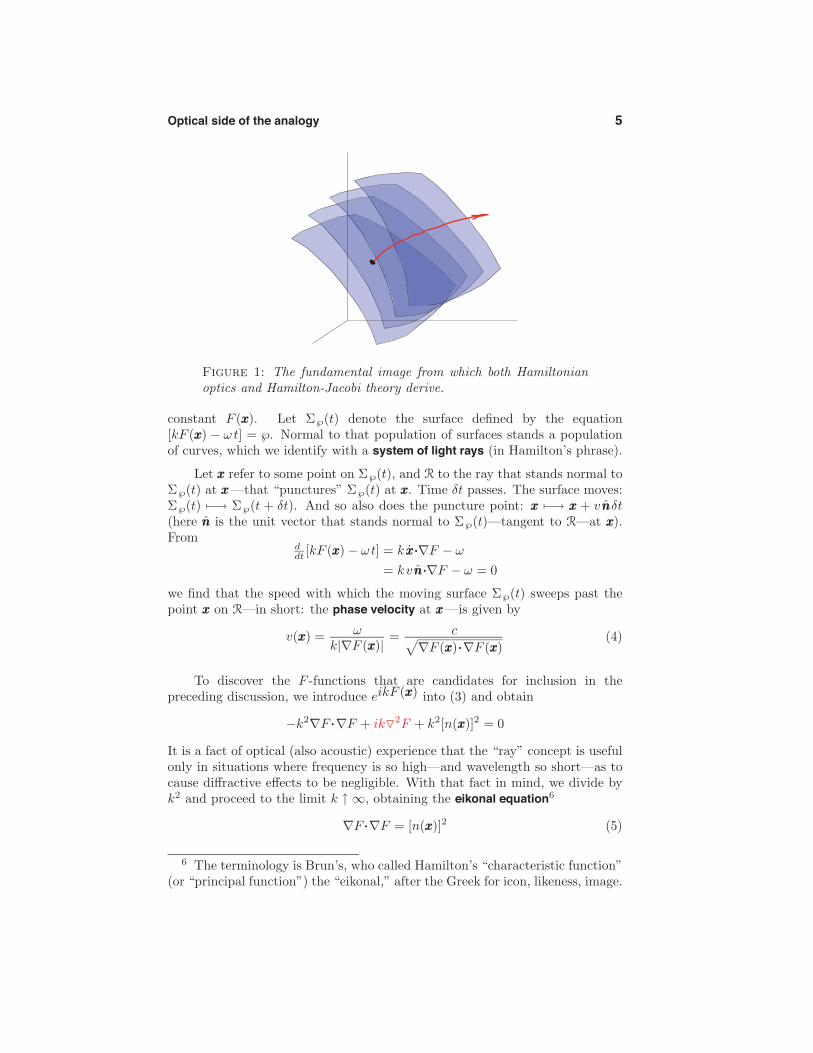
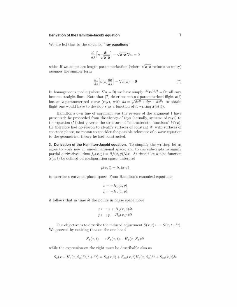
Figure 1: The fundamental image from which both Hamiltonianoptics and Hamilton-Jacobi theory derive.

constant F (xxx). Let Σ℘(t) denote the surface defined by the equation[kF (xxx) − ωt] = ℘. Normal to that population of surfaces stands a populationof curves, which we identify with a system of light rays (in Hamilton’s phrase).

Let xxx refer to some point on Σ℘(t), and R to the ray that stands normal toΣ℘(t) at xxx—that “punctures” Σ℘(t) at xxx. Time δt passes. The surface moves:Σ℘(t) �−→ Σ℘(t + δt). And so also does the puncture point: xxx �−→ xxx + vnnnδt(here nnn is the unit vector that stands normal to Σ℘(t)—tangent to R—at xxx).From

ddt [kF (xxx) − ωt] = kxxx···∇F − ω

= kvnnn···∇F − ω = 0

we find that the speed with which the moving surface Σ℘(t) sweeps past thepoint xxx on R—in short: the phase velocity at xxx—is given by

v(xxx) = ωk|∇F (xxx)| = c√

∇F (xxx)···∇F (xxx)(4)

To discover the F -functions that are candidates for inclusion in thepreceding discussion, we introduce eikF (xxx) into (3) and obtain

−k2∇F ···∇F + ik�2F + k2[n(xxx)]2 = 0

It is a fact of optical (also acoustic) experience that the “ray” concept is usefulonly in situations where frequency is so high—and wavelength so short—as tocause diffractive effects to be negligible. With that fact in mind, we divide byk2 and proceed to the limit k ↑ ∞, obtaining the eikonal equation6

∇F ···∇F = [n(xxx)]2 (5)

6 The terminology is Brun’s, who called Hamilton’s “characteristic function”(or “principal function”) the “eikonal,” after the Greek for icon, likeness, image.


This non-linear partial differential equation is structurally identical to (4),which can be written

[c/v(xxx)]2 = ∇F ···∇F (6)

But at (4) we imagined ourselves to be evaluating v(xxx) after F (xxx) has beenprescribed, while at (5) it is n(xxx) that has been prescribed, and F (xxx) that isbeing evaluated. Taken together, the two statements imply that “phase velocityat xxx” has meaning irrespective of which ray R through xxx one has in mind,and irrespective also of the specific “system of rays” that one has supposedcontains R as a member—irrespective, that is to say, of the global geometryof the surfaces-of-constant-F from which that system (or “pencil”) of rays hasbeen assumed to radiate.

That geometrical optics can be formulated as a theory of surfaces (surfacesof constant F (xxx), with F (xxx) subject to (5)), with rays standing everywherenormal to those surfaces,7 was first appreciated by Hamilton, rediscovered byBruns.

The established properties of those surfaces permit one to say sharp thingsabout the associated rays. Let ray R stand normal to Σ℘(0) at xxxA, let xxxB marksome down-stream point on R, and let xxx(λ) provide a parametric descriptionof the ray: xxx(0) = xxxA and xxx(1) = xxxB . We watch the motion of the puncturepoint produced by the advancing surface Σ℘(t). Specifically, we compute thetime of flight xxxA −→ xxxB :

T [xxxA −−−−−−−−→along ray

xxxB ] =∫ 1

0

1v(xxx(λ))

√xxx(λ)···xxx(λ) dλ : xxx(λ) ≡ dxxx(λ)

dλ

= 1c

∫n(xxx)

√xxx···xxx dλ

= “optical length” of the ray segmentc

It follows from the fact that the puncture point advances always normally toΣ℘(t)—which is to say: along the locally shortest path from xxx on Σ℘(t) toΣ℘(t + δt)—that the time of flight along the ray xxxA −→ xxxB is shorter thanwould be the time of flight along any alternative curve linking those points.Thus have we recovered Fermat’s principle of least time. Geometrical opticsis, however, a theory of curves and surfaces in which time plays actually norole (Fermat worked before it had been established experimentally that it evenmade sense to speak of a finite “speed of light”): what we are really talkingabout here is a principle of shortest optical length. In any event, from

δ

∫n(xxx)

√xxx···xxx dλ = 0

it follows that {ddλ

∂∂xxx

− ∂∂xxx

}n(xxx)

√xxx···xxx = 000

7 The imagery is not at all unfamiliar: think of the “lines of force” that standeverywhere normal to “surfaces of constant potential.”

Derivation of the Hamilton-Jacobi equation 7

We are led thus to the so-called “ray equations”

ddλ

[n xxx√

xxx···xxx

]−√

xxx···xxx∇n = 0

which if we adopt arc-length parameterization (where√

xxx···xxx reduces to unity)assumes the simpler form

dds

[n(xxx)dxxx

ds

]−∇n(xxx) = 000 (7)

In homogeneous media (where ∇n = 000) we have simply d2xxx/ds2 = 000 : all raysbecome straight lines. Note that (7) describes not a t-parameterized flight xxx(t)but an s-parameterized curve (ray), with ds =

√dx2 + dy2 + dz2: to obtain

flight one would have to develop s as a function of t, writing xxx(s(t)).

Hamilton’s own line of argument was the reverse of the argument I havepresented: he proceeded from the theory of rays (actually, systems of rays) tothe equation (5) that governs the structure of “characteristic functions” W (xxx).He therefore had no reason to identify surfaces of constant W with surfaces ofconstant phase, no reason to consider the possible relevance of a wave equationto the geometrical theory he had constructed.

3. Derivation of the Hamilton-Jacobi equation. To simplify the writing, let usagree to work now in one-dimensional space, and to use subscripts to signifypartial derivatives: thus fx(x, y) = ∂f(x, y)/∂x. At time t let a nice functionS(x, t) be defined on configuration space. Interpret

p(x, t) = Sx(x, t)

to inscribe a curve on phase space. From Hamilton’s canonical equations

x = +Hp(x, p)p = −Hx(x, p)

it follows that in time δt the points in phase space move

x �−→x + Hp(x, p)δtp �−→ p − Hx(x, p)δt

Our objective is to describe the induced adjustment S(x, t) �−→ S(x, t+δt).We proceed by noticing that on the one hand

Sx(x, t) �−→ Sx(x, t) − Hx(x, Sx)δt

while the expression on the right must be describable also as

Sx(x + Hp(x, Sx)δt, t + δt) = Sx(x, t) + Sxx(x, t)Hp(x, Sx)δt + Sxt(x, t)δt


p − Hx(x, p)δt

p

x x + Hp(x, p)δt

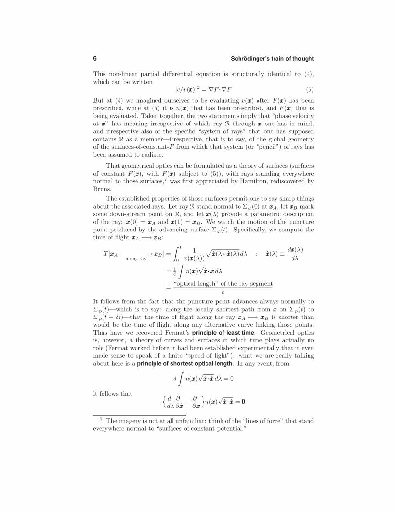
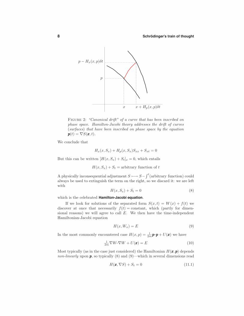
Figure 2: “Canonical drift” of a curve that has been inscribed onphase space. Hamilton-Jacobi theory addresses the drift of curves(surfaces) that have been inscribed on phase space by the equationppp(t) = ∇S(xxx, t).

We conclude that

Hx(x, Sx) + Hp(x, Sx)Sxx + Sxt = 0

But this can be written [H(x, Sx) + St]x = 0, which entails

H(x, Sx) + St = arbitrary function of t

A physically inconsequential adjustment S �−→ S−∫ t(arbitrary function) could

always be used to extinguish the term on the right, so we discard it: we are leftwith

H(x, Sx) + St = 0 (8)

which is the celebrated Hamilton-Jacobi equation.If we look for solutions of the separated form S(x, t) = W (x) + f(t) we

discover at once that necessarily f(t) = constant, which (partly for dimen-sional reasons) we will agree to call E. We then have the time-independentHamiltonian-Jacobi equation

H(x, Wx) = E (9)

In the most commonly encountered case H(x, p) = 12mppp···ppp + U(xxx) we have

12m∇W···∇W + U(xxx) = E (10)

Most typically (as in the case just considered) the Hamiltonian H(xxx, ppp) dependsnon-linearly upon ppp, so typically (8) and (9)—which in several dimensions read

H(xxx,∇S) + St = 0 (11.1)

Completion of the optico-mechanical analogy 9

andH(xxx,∇W ) = E (11.2)

with S = S(xxx, t) and W = W (xxx)—are non-linear partial differential equations.

The Newtonian, Lagrangian and canonical formalisms culminate in systems—often quite large systems—of coupled ordinary differential equations. It isremarkable that in (11) all that physics has come to rest in a single partialdifferential equation, and noteworthy that, while it is ∇U that enters into theequations of motion supplied by the formalisms just mentioned, U(xxx) entersnakedly/undifferentiatedly into the Hamilton-Jacobi equation. . . as it will alsointo the Schrodinger equation.

It is upon the foundation provided by the elegant material just presented—a body of theory that was more than ninety years old by the time he decidedto accept de Broglie/Einstein’s challenge—that Schrodinger erected his “wavemechanics.”

4. Completion of the optico-mechanical analogy. Note first that from p = Sx itfollows that dimensionally

[S ] = (length)(momentum) = action = [� ]

Pursuing now in reverse the change of dependent variable that led us from (2)to (5/6), we write

ψ(xxx, t) = ψ0 eiS(xxx, t)/� (12)

and observe that

− �2

2m�2ψ =

{1

2m∇S ···∇S − i �

2m�2S

}· ψ

Uψ ={

U}· ψ

−i�∂tψ ={

St

}· ψ

from which it follows (by i(�/2m)ψ�2S = (�2/2m)ψ�2 log[ψ/ψ0]) that

− �2

2m

[�2ψ − ψ�2 log[ψ/ψ0]

]+ Uψ − i�ψt =

{1

2m∇S ···∇S + U + St

}· ψ

We conclude that the equation

− �2

2m

[�2ψ − ψ�2 log[ψ/ψ0]

]+ Uψ − i�ψt = 0

is but a renotated variant of—and entirely equivalent to—the Hamilton-Jacobiequation, an eccentric way of rendering classical mechanics. Schrodinger had,however, the wit to abandon the ψ�2 log[ψ/ψ0] term. He was left then with a


linear field equation (we know that linearity in quantum mechanics is the nameof the game!)—the time-dependent Schrodinger equation

− �2

2m�2ψ + Uψ = i�ψt (13)

which is manifestly not just old wine in a new bottle.

It is instructive to pursue the preceding argument in reverse: insert8

ψ(xxx, t) = R(xxx, t) e iS(xxx, t)/�

into the Schrodinger equation (13) and obtain an equation the real andimaginary parts of which can be written

12m∇S ···∇S + U(xxx) − �

2

2m�2RR

+ St = 0 (14.1)

∂tR2 + ∇···

[1mR2∇S

]= 0 (14.2)

respectively. These coupled equations are—conjointly—entirely equivalent tothe Schrodinger equation. The latter possesses the form

∂∂t (density) + ∇···(current) = 0 : density = R2 = ψ∗ψ

of a “continuity equation,” and evidently describes the local conservation ofprobability.9 Equation (14.1) gives back the Hamilton-Jacobi in the classicallimit � ↓ 0. Recall that a limiting process entered also into the derivation ofthe eikonal equation (5) from the wave equation (2).

Curiously, one might look upon the Schrodinger equation as a “linearizedHamilton-Jacobi equation.” Even if the quantum world did not exist, it wouldmake computational good sense to adopt the following 3-step program

• linearize• solve the resulting “Schrodinger equation”• proceed to the classical limit � ↓ 0

as a way of solving classical problems.

If one introduces the time-separated wave function

ψ(xxx, t) = R(xxx)e i[W (xxx) − Et]/�

into the Schrodinger equation (16) one obtains

12m∇W ···∇W = E − U(xxx) + �

2

2m�2RR

(15.1)

∇···[

1mR2∇W

]= 0 (15.2)

8 We use this polar alternative to (12) to insure the reality of R(xxx, t) andS(xxx, t).

9 Note that Schrodinger’s derivation of (13) did not carry with it anyinterpretive advice. Nor did it have anything to say about the (very unclassical)quantum measurement process: all of that came later (Born, von Neumann).

“Rays” traced by classical particles 11

In the classical limit the former equation decouples, to give back the time-independent Hamilton-Jacobi equation (10):

∇W ···∇W = 2m[E − U(xxx)]

5. The “rays” traced by classical particles. We now take leave of Schrodingerto trace this story back to point of departure. In recent discussion we haveproceeded

classical H-J theory −−−−−−−−−−−−→ quantum wave theory

and I propose now to proceed in the reverse direction:

classical particle trajectories ←−−−−−−−−−−−− classical H-J theory

It is by way of preparation that we distinguish several “natural velocities”(speeds) that arise from the theory of waves and particles.

Recall that the phase velocity of the simple wave ei[kx − ω(k)t], got bysetting d

dt [kx − ω(k)t] = 0, is given by

vphase =ω(k)

k

while the group velocity, got by looking to the motion of the envelope whensuch waves of nearly identical k-values are superimposed,10 is given by

vgroup =dω(k)

dk

If we use de Broglie’s relations E = hν = � ω and p = h/λ = �k to translatethose equations into mechanical variables we obtain

vphase =E(p)

p

vgroup =dE(p)

dp

which in the case E(p) = 12mp2 + U become

vphase(xxx) = E√2m[E − U(xxx)]

vgroup(xxx) = 1mp = 1

m

√2m[E − U(xxx)]

Recall also that a mass point m, if moving with conserved energy E in the

10 See Chapter 6, §5 in my sophomore notes (2005).


presence of a potential U(xxx), necessarily has speed

vE(xxx) =√

2m [E − U(xxx)]

when it passes through point xxx, whatever the direction in which it is moving.That

vE(xxx) = vgroup(xxx)

conforms to our experience that in quantum mechanics classical particle motionis represented by the motion of wave packets.

In “Geometrical mechanics: remarks commemorative of Heinrich Hertz”11

I show it to be an implication of Newton’s myyy(t) = −∇U(yyy) that one canalways write yyy(t) = xxx(s(t)) where

• xxx(s) describes the path traced by the particle (mechanical analog of a“ray”) and s signifies Euclidean arc length ;

• s(t) describes progress along that path, and is got by integrating s = vE(xxx).I am able to show, moreover, that xxx(s) satisfies a set of equations

dds

[n(xxx)dxxx

ds

]−∇n(xxx) = 000 (16)

that is structurally identical to the ray equations (7), except that here

n(xxx) = cvphase(xxx)

=

√2mc2[E − U(xxx)]

E=

√2mc2

E

√kinetic energy T

where physically inconsequential factors have been introduced simply to rendern(xxx) dimensionless, and to highlight the formal identity of the mechanicalequation with its optical counterpart. It follows already from our previouswork that (16) can be obtained from12

δE

∫n(xxx(s))ds ∼ δE

∫ √T ds ∼ δE

∫T dt

This variational principle, first stated by Jacobi and later by Hertz, is the directmechanical analog of Fermat’s Principle of Least Time. Neither principle hasanything to do with time or motion: both have to do with the design of curves,rays, trajectories, “flight paths.” The Jacobi-Hertz principle of least actionstates that of all curves that are pursued xxxA −→ xxxB with constant energy E,the curve realized by a particle in natural motion will be the one that extremizesthe mechanical analog of optical path length.13

All of which emerges quite naturally when (with Hamilton) we identifythose curves with the curves normal to surfaces of constant S(xxx, t) = W (xxx)−Etand observe that those surfaces advance with speed

v(xxx) = E√∇W···∇W

= E√2m[E − U(xxx)]

= vphase(xxx)

11 Notes for a Reed College Physics Seminar presented 23 February 1994.12 The final step here follows from s2 = m

2 T ; i.e., from ds ∼√

T dt.13 For detailed discussion see H. Goldstein, C. Poole & J. Safko, Classical

Mechanics (3rd edition 2002), §8.6.

“Rays” traced by classical particles 13

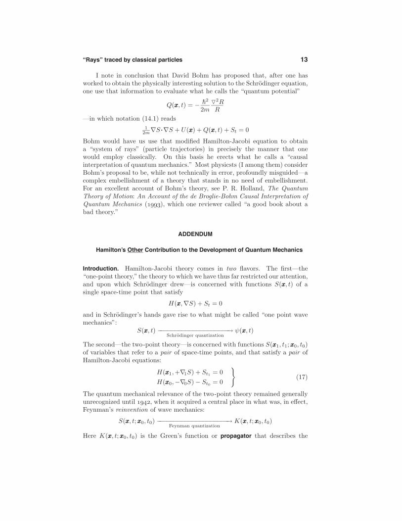
I note in conclusion that David Bohm has proposed that, after one hasworked to obtain the physically interesting solution to the Schrodinger equation,one use that information to evaluate what he calls the “quantum potential”

Q(xxx, t) = − �2

2m�2RR

—in which notation (14.1) reads1

2m∇S ···∇S + U(xxx) + Q(xxx, t) + St = 0

Bohm would have us use that modified Hamilton-Jacobi equation to obtaina “system of rays” (particle trajectories) in precisely the manner that onewould employ classically. On this basis he erects what he calls a “causalinterpretation of quantum mechanics.” Most physicsts (I among them) considerBohm’s proposal to be, while not technically in error, profoundly misguided—acomplex embellishment of a theory that stands in no need of embellishment.For an excellent account of Bohm’s theory, see P. R. Holland, The QuantumTheory of Motion: An Account of the de Broglie-Bohm Causal Interpretation ofQuantum Mechanics (1993), which one reviewer called “a good book about abad theory.”

ADDENDUM

Hamilton’s Other Contribution to the Development of Quantum Mechanics

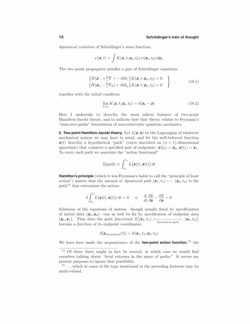
Introduction. Hamilton-Jacobi theory comes in two flavors. The first—the“one-point theory,” the theory to which we have thus far restricted our attention,and upon which Schrodinger drew—is concerned with functions S(xxx, t) of asingle space-time point that satisfy

H(xxx,∇S) + St = 0

and in Schrodinger’s hands gave rise to what might be called “one point wavemechanics”:

S(xxx, t) −−−−−−−−−−−−−−−−−−−−→Schrodinger quantization

ψ(xxx, t)

The second—the two-point theory—is concerned with functions S(xxx1, t1;xxx0, t0)of variables that refer to a pair of space-time points, and that satisfy a pair ofHamilton-Jacobi equations:

H(xxx1,+∇1S) + St1 = 0H(xxx0,−∇0S) − St0 = 0

}(17)

The quantum mechanical relevance of the two-point theory remained generallyunrecognized until 1942, when it acquired a central place in what was, in effect,Feynman’s reinvention of wave mechanics:

S(xxx, t;xxx0, t0) −−−−−−−−−−−−−−−−−−−−→Feynman quantization

K(xxx, t;xxx0, t0)

Here K(xxx, t;xxx0, t0) is the Green’s function or propagator that describes the


dynamical evolution of Schrodinger’s wave function:

ψ(xxx, t) =∫

K(xxx, t;xxx0, t0)ψ(xxx0, t0) dxxx0

The two-point propagator satisfies a pair of Schrodinger equations{H(xxx ,+�

i ∇ ) − i�∂t

}K(xxx, t;xxx0, t0) = 0{

H(xxx0,−�

i ∇0) + i�∂t0

}K(xxx, t;xxx0, t0) = 0

}(18.1)

together with the initial condition

limt↓t0

K(xxx, t;xxx0, t0) = δ(xxx0 − xxx) (18.2)

Here I undertake to describe the most salient features of two-pointHamilton-Jacobi theory, and to indicate how that theory relates to Feynman’s“sum-over-paths” formulation of non-relativistic quantum mechanics.

5. Two-point Hamilton-Jacobi theory. Let L(xxx, xxx) be the Lagrangian of whatevermechanical system we may have in mind, and let the well-behaved functionxxx(t) describe a hypothetical “path” (curve inscribed on (n + 1)-dimensionalspacetime) that connects a specified pair of endpoints: xxx(t0) = xxx0, xxx(t1) = xxx1.To every such path we associate the “action functional”

S[path] ≡∫ t1

t0

L(xxx(t), xxx(t)

)dt

Hamilton’s principle (which it was Feynman’s habit to call the “principle of leastaction”) asserts that the natural or dynamical path (xxx1, t1) ←− (xxx0, t0) is thepath14 that extremizes the action:

δ

∫ t1

t0

L(xxx(t), xxx(t)

)dt = 0 ⇒ d

dt∂L∂xxx

− ∂L∂xxx

= 0

Solutions of the equations of motion—though usually fixed by specificiationof initial data (xxx0, xxx0)—can as well be fix by specification of endpoint data(xxx0, xxx1). Thus does the path functional S

[(xxx1, t1) ←−−−−−−−−−−−−

dynamical path(xxx0, t0)

]become a function of its endpoint coordinates:

S[xxxdynamical(t)] = S(xxx1, t1;xxx0, t0)

We have here made the acquaintance of the two-point action function,15 the

14 Of these there might in fact be several, in which case we would findourselves talking about “local extrema in the space of paths.” It serves mypresent purposes to ignore that possibility.

15 . . .which in cases of the type mentioned in the preceding footnote may bemulti-valued.

2-point Hamilton-Jacobi theory 15

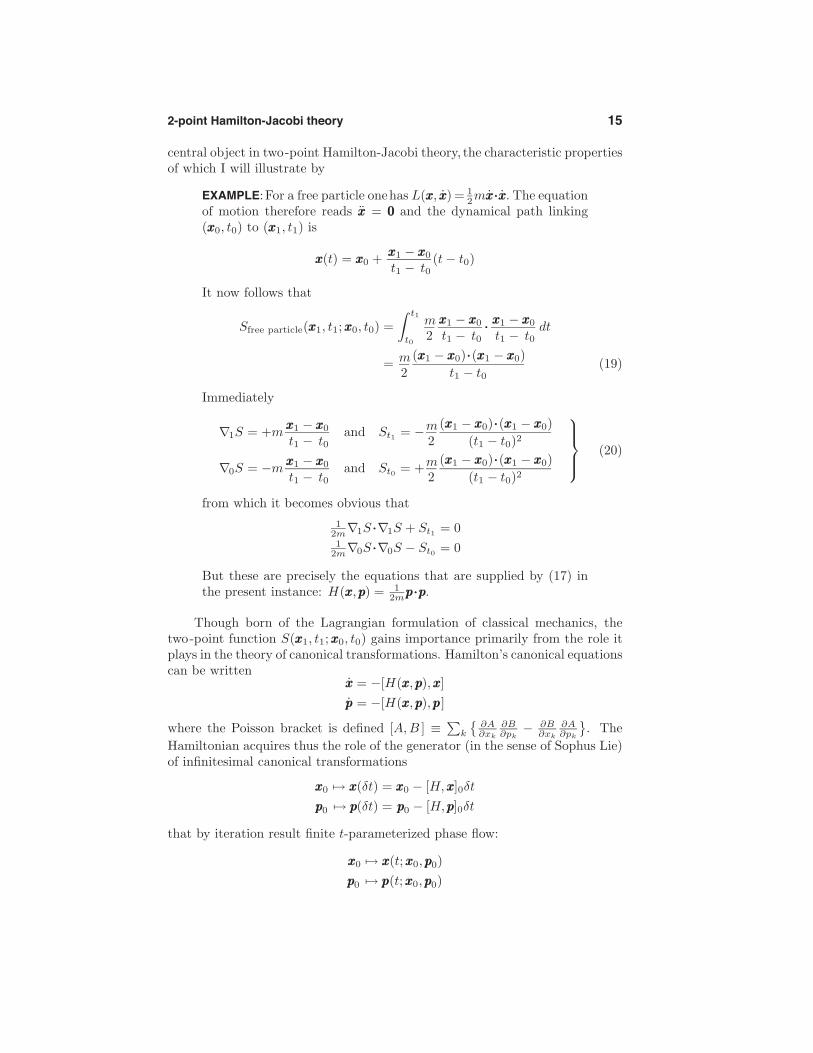
central object in two-point Hamilton-Jacobi theory, the characteristic propertiesof which I will illustrate by

EXAMPLE:For a free particle onehas L(xxx, xxx) = 12mxxx···xxx. The equation

of motion therefore reads xxx = 000 and the dynamical path linking(xxx0, t0) to (xxx1, t1) is

xxx(t) = xxx0 + xxx1 − xxx0

t1 − t0(t − t0)

It now follows that

Sfree particle(xxx1, t1;xxx0, t0) =∫ t1

t0

m2

xxx1 − xxx0

t1 − t0··· xxx1 − xxx0

t1 − t0dt

= m2

(xxx1 − xxx0)···(xxx1 − xxx0)t1 − t0

(19)

Immediately

∇1S = +mxxx1 − xxx0

t1 − t0and St1 = −m

2(xxx1 − xxx0)···(xxx1 − xxx0)

(t1 − t0)2

∇0S = −mxxx1 − xxx0

t1 − t0and St0 = +m

2(xxx1 − xxx0)···(xxx1 − xxx0)

(t1 − t0)2

⎫⎪⎪⎬⎪⎪⎭ (20)

from which it becomes obvious that1

2m∇1S ···∇1S + St1 = 01

2m∇0S ···∇0S − St0 = 0

But these are precisely the equations that are supplied by (17) inthe present instance: H(xxx, ppp) = 1

2mppp···ppp.

Though born of the Lagrangian formulation of classical mechanics, thetwo-point function S(xxx1, t1;xxx0, t0) gains importance primarily from the role itplays in the theory of canonical transformations. Hamilton’s canonical equationscan be written

xxx = −[H(xxx, ppp), xxx]ppp = −[H(xxx, ppp), ppp ]

where the Poisson bracket is defined [A, B ] ≡∑

k

{∂A∂xk

∂B∂pk

− ∂B∂xk

∂A∂pk

}. The

Hamiltonian acquires thus the role of the generator (in the sense of Sophus Lie)of infinitesimal canonical transformations

xxx0 �→ xxx(δt) = xxx0 − [H,xxx]0δtppp0 �→ ppp(δt) = ppp0 − [H,ppp]0δt

that by iteration result finite t-parameterized phase flow:

xxx0 �→ xxx(t;xxx0, ppp0)ppp0 �→ ppp(t;xxx0, ppp0)


The function S(xxx, t;xxx0, 0) achieves that same finitistic result by different means:write

ppp = ppp (xxx, t;xxx0, t0) = +∇ S(xxx, t;xxx0, t0)ppp0 = ppp0(xxx, t;xxx0, t0) = −∇0S(xxx, t;xxx0, t0)

By functional inversion (often more easily said than done!) of the latter equationobtain

xxx = xxx(t;xxx0, ppp0, t0)

Then return with that information to the first equation to obtain

ppp = ppp(t;xxx0, ppp0, t0)

We recognize the sequence of operations just described to comprise an instanceof Legendre’s procedure for promoting derivatives to the status of independentvariables. Evidently

• the Hamiltonian H(xxx, ppp) is the Lie generator of dynamical flow in phasespace, and does its work incrementally;

• the two-point action function S(xxx, t;xxx0, t0) is the Legendre generator ofthat evolving canonical transformation, and does its work wholistically

and the Hamilton-Jacobi equations (17) describe the relationship between thosegenerators.

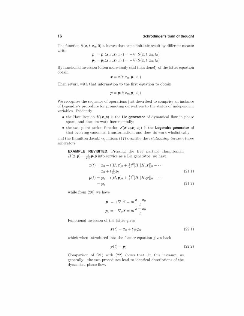
EXAMPLE REVISITED: Pressing the free particle HamiltonianH(xxx, ppp) = 1

2mppp···ppp into service as a Lie generator, we have

xxx(t) = xxx0 − t[H,xxx ]0 + 12 t2[H, [H,xxx ]]0 − · · ·

= xxx0 + t 1m ppp0 (21.1)

ppp(t) = ppp0 − t[H,ppp ]0 + 12 t2[H, [H,ppp ]]0 − · · ·

= ppp0 (21.2)

while from (20) we have

ppp = +∇ S = mxxx − xxx0

t

ppp0 = −∇0S = mxxx − xxx0

t

Functional inversion of the latter gives

xxx(t) = xxx0 + t 1m ppp0 (22.1)

which when introduced into the former equation gives back

ppp(t) = ppp0 (22.2)

Comparison of (21) with (22) shows that—in this instance, asgenerally—the two procedures lead to identical descriptions of thedynamical phase flow.

Feynmanism 17

It is obvious—yet instructive to notice—that two-point functions becomesingle-point functions (of a certain type) when the second argument is frozen:S(xxx, t; •, •) = S(xxx, t). Such neutered functions are, however, incapable ofgenerating canonical transformations. I note also that constants of the motionarise within H-theory from conditions of the form [H, A ] = 0 , but in S-theoryfrom symmetries of the two-point action (Noether’s theorem), but will refrainfrom discussion of how those two notions come to be interconnected.

6. Quantum mechanics according to Feynman. The train of thought that ledthe 23-year-old Richard Feynman (1918–1988) to his very fruitful reinvention ofnon-relativistic quantum mechanics can be traced to an occasion when he askeda drinking buddy whether he “had ever encountered a quantum mechanicalapplication of the principle of least action” (his allusion being actually toHamilton’s principle), and was referred to an obscure paper by P.A.M. Dirac.16

The objects of central interest to Dirac (as also to Feynman after him) werenot “one-point Schrodinger functions” ψ(xxx, t) but the “two-point Schrodingerfunctions” K(xxx, t;xxx0, t0) that arise in xxx-representation

K(xxx, t;xxx0, t0) = (xxx |U(t; t0)|xxx0)

of the unitary operator that (in the Schrodinger picture) sends |ψ)t0 �−→ |ψ)t,and that, as was remarked at (18), become single-point functions (of a certaintype) when the second argument is frozen: K(xxx, t; •, •) = ψ(xxx, t).

Necessarily

U(t1; t0) = U(t1; t)U(t; t0) : t1� t � t0

which in xxx-representation becomes the slightly less obvious composition rule

K(xxx1, t1;xxx0, t0) =∫

K(xxx1, t1;xxx, t) dxxxK(xxx, t;xxx0, t0)

Feynman—typically—attached to that equation a much more robustly physicalinterpretation than Dirac, in his sophistication, had reason to do:17 Feynmanconsidered it to state that

probability amplitude of transition (xxx1, t1) ←− (xxx0, t0)

=∫ {

amplitude of transition via the intermediate point (xxx, t)}

dxxx

16 “The Lagrangian in quantum mechanics,” Physikalische Zeitschrift derSowjetunion 3, 1933. This beautiful paper is reprinted in J. Schwinger (editor),Selected Papers on Quantum Mechanics (1958)—a valuable collection of classicpapers known commonly as “the Schwinger collection.”

17 Dirac, working in the Heisenberg picture, looked upon (xxx1, t1|xxx0, t0) as anelement of a transformation matrix that relates one representation to another.


Dirac noted—and Feynman later made much of the fact— that by repeatedapplication of the composition rule one can resolve K(xxx1, t1;xxx0, t0) into iteratedshort-time propagators

K(xxx1, t1;xxx0, t0) =∫· · ·

∫K(xxx1, t1;yyyN , t1 − τ) dyyyN · · · dyyy1K(yyy1, t0 + τ ;xxx0, t0)

Dirac—who considered himself to be simply pointing out a formal parallelismbetween quantum mechanical transformation theory (in the development ofwhich he had played the leading role) and the classical theory of canonicaltransformations—was led at this point to remark that

K(yyy, t + τ ;xxx, t) “corresponds to” eiS(yyy, t + τ ;xxx, t)/�

and that therefore K(xxx1, t1;xxx0, t0) “corresponds (in the limit N ↑ ∞) to”∫· · ·

∫eiS(xxx1, t1;yyyN , t1 − τ)/� dyyyN · · · dyyy1e

iS(yyy1, t0 + τ ;xxx0, t0)/�

=∫· · ·

∫exp

{(i/�)

∫ t1

t0

L(xxx1 ←−−−−−−−−−−−−yyyN ,...,yyy2,yyy1

xxx0) dt}

dyyyN · · · dyyy1

where τ = t1 − t0N+1

and xxx1 ←−−−−−−−−−−−−yyyN ,...,yyy2,yyy1

xxx0 refers to the segmented path

xxx1 ←− xxx0 that visits successively the points{yyyN , . . . , yyy2, yyy1

}. Dirac found

it natural, in view of his objective, to point out (without explicit referenceto the method of stationary phase) that in the classical limit � ↓ 0 the pathscontemplated above tend collectively to “buzz themselves to extinction,” theonly path immune to this fate being the path (or paths) whose nodal-points{yyyN , . . . , yyy2, yyy1

}are so placed as to extremize18

S(xxx1 ←−−−−−−−−−−−−yyyN ,...,yyy2,yyy1

xxx0) =N∑

n=0

S(yyyn+1, tn + τ ;yyyn, tn)

—placed, that is to say, so as to lie on the classical path (xxx1, t1) ← (xxx0, t0).

Feynman—mystified by Dirac’s “corresponds to”—chose tentatively tointerpret that phrase to mean “equals”(actually: “equals to within an adjustablefactor”) and to see where he was led. Setting

K(yyy, t + τ ;xxx, t) = 1A(τ)

eiS(yyy, t + τ ;xxx, t)/� (23)

his conjecture read

K(xxx1, t1;xxx0, t0) (24)

= limN↑∞

∫· · ·

∫ N∏n=0

1A(τ)

eiS(yyyn+1, tn + τ ;yyyn, tn)/� dyyy1dyyy2 · · · dyyyN

18 Here yyy0 ≡ xxx0, yyyN+1 ≡ xxx1 and tn = t0 + nτ .

Feynmanism 19

Proceeding in the one-dimensional case from the assumption that

L(x, x) = 12mx2 − V (x)

Feynman was able to establish in fairly short order (which is to say: by heavycalculation completed within hours of his first reading of Dirac’s paper) that if(24) is used to construct the propagator K(x, t;x0, t0) that appears in

ψ(x, t) =∫

K(x, t;x0, t0)ψ(x0, t0) dx0

then the resulting ψ(x, t) does in fact satisfy the Schrodinger equation, and doesin fact give back ψ(x0, t0) as t ↓ t0.19

EXAMPLE: For a free particle it was established already at(19) that

S(x1, t0 + τ ;x0, t0) =m(x1 − x0)2

2τ

so in this instance (23) reads

K(x1, t0 + τ ;x0, t0) = 1A(τ)

eim(x1 − x0)2/2�τ

= 1A(τ)

√πσ · 1√

πσe−(x1 − x0)2/σ

σ ≡ 2i�τ/m

With Feynman we temporarily complexify �

� �−→ � − iε : ε > 0

so as to render the real part of σ positive. This done, we have

∫ +∞

−∞

1√πσ

e−(x1 − x0)2/σ dx1 = 1

and recognize the integrand to provide (in the limit σ ↓ 0) aGaussian representation of δ(x1 − x0). We therefore have, as wasrequired at (18.2),

limτ↓0

K(x1, t0 + τ ;x0, t0) = δ(x1 − x0) (25)

provided we setA(τ) =

√πσ =

√ihτ/m

19 For proof see pages 29–30 in Chapter 3 of advanced quantum topics(2000).


Observe next that∫ +∞

−∞

1√πσ

e−(x1 − y)2/σ 1√πσ

e−(y − x0)2/σ dy

= 1√π2σ

e−(x1 − x0)2/2σ

and that N -fold iteration of this result would lead Feynman to write

K(x1, t1;x0, t0) = limN↑∞

1√π(N + 1)σ

e−(x1 − x0)2/(N + 1)σ

= 1√ih(t1− t0)/m

e(i/�)m(x1 − x0)2/2(t1− t0) (26)

We verify by quick calculation that the expression on the right doesin fact satisfy the free particle Schrodinger equations (18.1)

{− �

2

2m∂2x1

− i�∂t1

}K(x1, t1;x0, t0) = 0{

− �2

2m∂2x0

+ i�∂t0

}K(x1, t1;x0, t0) = 0

EXAMPLE: For an oscillator —assuming classical motionto be uniform in the short term

x(t) = x0 + x1 − x0

τ(t − t0) : t0 � t � t0 + τ

—we compute

S(x1, t0 + τ ;x0, t0)

=∫ t0+τ

t0

{12m

[x1 − x0

τ

]2

− 12mω2

[x0 + x1 − x0

τ(t − t0)

]2}

dt

=m(x1 − x0)2

2τ− mω2τ

6(x2

1 + x1x0 + x20

)(27)

A moment’s thought shows that to recover (25) we have again toset A(τ) =

√ihτ/m, and so have

K(x1, t0 + τ ;x0, t0) (28)

= 1√ihτ/m

exp{

i�

[m(x1 − x0)2

2τ− mω2τ

6(x2

1 + x1x0 + x20

)]}

Introduction of this result into Feynman’s formula (24) leads (aftercomplexification of �) to a multiple integral that can be managedeffectivelybyappeal to the N -dimensional Gaussian integral formula

∫· · ·

∫ +∞

−∞eixxx···yyye−

12yyy···Ayyydy1dy2 · · · dyN =

(2π)N/2

√det A

e−12xxx···A–1xxx

Feynmanism 21

Taking the result to the limit N ↑ ∞ requires a bit of finesse (forthese and other computational details see pages 43–47 in Chapter 3of my advanced quantum topics (2000)), but leads ultimatelyto the formula

K(x1, t1;x0, t0) (29)

=√

mωih sin ω(t1−t0)

exp{

i�

mω2 sin ω(t1−t0)

[(x2

1+x20) cos ω(t1−t0)−2x1x0

]}

from which, it is gratifying to observe, we recover (26) as ω ↓ 0.Computation establishes that the Feynman’s oscillator propagator(29) satisfies

{− �

2

2m∂2x1

+ 12mω2x2

1 − i�∂t1

}K(x1, t1;x0, t0) = 0{

− �2

2m∂2x0

+ 12mω2x2

0 + i�∂t0

}K(x1, t1;x0, t0) = 0

Feynman’s central idea, as set forth in his thesis (May 1942) and in thepaper which he published (Reviews of Modern Physics, 1948),20 admits of thepicturesque if somewhat imprecise formulation

K(xxx, t;xxx0, t0) =∫

all paths

ei�

∫L(path) dt D[paths] (30)

which he interprets to describe a sum over the probability amplitudes that hewould associate with each conceivable path (xxx, t) ←− (xxx0, t0), his contentionbeing that each path contributes with the same weight, but with a phasedetermined by the classical action S[path] = i

�

∫L(path) dt. He shows how

(30) can be used to provide novel insight into the construction of• quantum mechanical conservation laws• commutation relations• expectation values.

Subsequent work by others established that (30) can be made to retainits accuracy even when the meaning of “all paths” is altered in various ways—the important implication being that Feynman’s success cannot be interpreted

20 The thesis is entitled “The principle of least action in quantum mechanics,”and in his abstract Feynman claims to have produced a generalization of thestandard Heisenberg/Schrodinger/Born theory. In the published version (whichis reprinted in the Schwinger collection) the title has been changed (to“Space-time approach to non-relativisticquantum mechanics”—the“space-time”evidently intended to draw attention to the fact that Feynman works throughoutin the xxx-representation, and the “non-relativistic” to disabuse readers of thepresumption that “space-time” means “spacetime”) and that claim is dropped:Feynman claims “no fundamentally new results,” aspires only to the “pleasureof recognizing old things from a new point of view.”


as having established that quantum particles do move xxx ←− xxx0 along diversenowhere-differentiable paths: it establishes only that they can be imagined todo so.

There remains—today as in 1942—no properly constructed general “theoryof functional integration” adequate to the work Feynman would have it do.Successful functional integrals appear in every instance to be Gaussian integrals,and to derive that characteristic from the fact that xxx enters quadratically intothe construction of physical Lagrangians. Feynman seems never to have beenmuch bothered by the fact that his physical intuition had carried him to a placebeyond the frontier of established mathematics, but. . .

Near the end of the conclusion to his thesis Feynman expresses his regretthat

“A point of vagueness is the normalizing factor, A. No rule hasbeen given to determine it for a given action expression. Thisquestion is related to the difficult mathematical question as to theconditions under which the limiting process of subdividing the timescale. . . actually converges.”

“Hamilton’s principle,” it has often been remarked—in the first instance byHamilton himself!—is due actually to Lagrange, whose work Hamilton held tobe a kind of “mathematical poem.” But it was Hamilton who first recognizedthat δ

∫L dt = 0 is but the point of entry into a rich landscape21 (theory of

canonical transformations, Hamilton-Jacobi theory) that emerges as soon asone looks to the properties of the functions S(xxx1, t1;xxx0, t0) that extremize thefunctional S[path] =

∫L dt. Feynman’s objective was, in a way, more restricted

than Dirac’s: he sought only to discover a natural place within quantum theoryfor the “principle of least action.” Had he not been so quick to dismiss thoseaspects of Dirac’s paper that drew upon the deeper reaches of Hamiltonianphysics he might well have resolved the problem identified in the precedingquotation—as, indeed, did others (Pauli 1951, Cecile Morette 1952) soon afterhim. I turn now to discussion of the relevant details.22

Working initially in one dimension, we proceed from

U(t + τ, t) = I − i

�Hτ + · · · ≈ e−iHτ/�

where H will be considered to have been obtained by xp-ordered substitutioninto the classical Hamiltonian H(x, p):

H =[

xH(x, p)

]p+ O(�)

21 Cornelius Lanczos, quoting from the Book of Exodus at the beginningof Chapter 8 in his Variational Principles of Mechanics (1949), refers to thislandscape as “holy ground.” Lanczos provides, by the way, an excellent accountof Hamilton-Jacobi theory that is directly relevant to many of the topicsdiscussed in the present essay.

22 The reader should be aware that my methods, taken from a notebook dated1971, are somewhat eccentric.

Feynmanism 23

In this notation

K(x, t + τ ;x0, t) =∫

(x|U(t + τ, t)|p)dp(p|x0)

≈∫

1h e

i�[(x−x0)p−τH(x,p)] dp

from which it follows in particular (and not at all surprisingly) that

limτ↓0

K(x, t + τ ;x0, t) =∫

1h e

i�(x−x0)p dp = δ(x − x0) : all H(x, p)

Notice now that [(x− x0)p− τH(x, p)] = τ [x−x0τ p−H(x, p)] is, by Hamilton’s

principle,23 stationary at the momentum pC associated with the classical path(x, t + τ) ← (x0, t), where it assumes the value S(x, t + τ ;x0, t). With thesepoints in mind, we use the method of stationary phase24 to obtain

lim�↓0

∫1h e

i�[(x−x0)p−τH(x,p)] dp ∼ 1

h

[ i2π�

−τHpp(x, p)

]12

eiS(x,t+τ ;x0,t)/�

∣∣∣∣p = p

C

Hamilton’s canonical equations of motion supply

x0 = x − τHp(x, p)∣∣∣p = p

C

giving∂x0

∂p= −τHpp(x, p)

∣∣∣p = p

C

whence1

−τHpp(x, p)= ∂p

∂x0

=∂2S(x, t + τ ;x0, t)

∂x∂x0

Assembling these results, we have

K(x, t + τ ;x0, t) =√

(i/h)D(x, t + τ ;x0, t) · eiS(x, t + τ ;x0, t)/�

D(x, t + τ ;x0, t) ≡∂2S(x, t + τ ;x0, t)

∂x∂x0

which in several dimensions becomes

K(xxx, t + τ ;xxx0, t) =√

(i/h)nD(xxx, t + τ ;xxx0, t) · eiS(xxx, t + τ ;xxx0, t)/� (31)

D(xxx, t + τ ;xxx0, t) ≡ det∥∥∥∂2S(xxx, t + τ ;xxx0, t)

∂xj∂xk0

∥∥∥EXAMPLE: For a free particle we on page 19 had

S(x1, t0 + τ ;x0, t0) =m(x1 − x0)2

2τ

23 Recall that L(x, x) = xp − H(x, p))24 See advanced quantum topics (2000), Chapter 0, page 47.


which is seen to give√

(i/h)D(x, t + τ ;x0, t) =√−im/hτ , in precise

agreement with Feynman’s 1/A(τ) =√

m/ihτ .

EXAMPLE: For an oscillator we on page 20 had

S(x1, t0 + τ ;x0, t0) =m(x1 − x0)2

2τ− mω2τ

6(x2

1 + x1x0 + x20

)

which gives√

(i/h)D(x, t + τ ;x0, t) =√−im/hτ [1 + 1

6 (ωτ)2]. This(in leading order) again reproduces Feynman’s normalization factor.

It is curious that Feynman himself seems to have been quite uninterested inthis work, though it resolves what he recognized to be a defect in his own work.It is neither cited nor exploited in Feynman & Hibbs, Quantum Mechanics andPath Integrals (1965).

The material sketched above refers to a property of the short-timepropagator K(x1, t0 + τ ;x0, t0). Interestingly, it can be considered to be aspecial consequence of a property of general propagators in the classical limit .If we write

K(xxx1, t1;xxx0, t0) = R(xxx1, t1;xxx0, t0) eiS(xxx1, t1;xxx0, t0)/�

then the argument that on page 10 gave (14) gives

12m∇1S ···∇1S + U(xxx1) + O(�2) + St1 = 0 (32.1)11

2m∇0S ···∇0S + U(xxx0) + O(�2) − St0 = 0 (32.1)0∇1 ···

[(1m∇1S

)R2

]+ ∂t1R

2 = 0 (32.2)1∇0 ···

[(1m∇0S

)R2

]− ∂t0R

2 = 0 (32.2)0

One can show25 that if the two-point function S(xxx1, t1;xxx0, t0) satisfies theHamilton-Jacobi equations (32.1)—with O(�2) terms omitted—then theVan Vleck determinant 26

D(xxx1, t1;xxx0, t0) ≡ det∥∥∥∂2S(xxx1, t1;xxx0, t0)

∂xj1∂xk

0

∥∥∥25 See advanced quantum topics (2000), Chapter 3, page 15. The

argument does not presume the Hamiltonian to have the specialized formH(xxx, ppp) = 1

2mppp···ppp + U(xxx) implicit in the way I have rendered equations (32).26 John Van Vleck (1899–1980) came upon this determinant in the course of

an early study of several-dimensional WKB theory (1928). In conversationwith me he once remarked that the idea sprang from a conversation withJ. R. Oppenheimer, and that his own contribution had been simply to workout the details. Van Vleck remarked with evident pride that the quantummechanical dissertation (1922) he wrote at Harvard (where he was the firststudent of E. C. Kemble) was an American first. He shared the Nobel Prize in1977.

Feynmanism 25

satisfies the continuity equations (32.2). This, I emphasize, is an entirelyclassical proposition, its quantum mechanical importance notwithstanding.

We are brought thus to the conclusion that the quantum propagatorK(xxx1, t1;xxx0, t0) can in semi-classical approximation be described

KC(xxx1, t1;xxx0, t0) =√

(i/h)nD(xxx1, t1;xxx0, t0) · eiS(xxx1, t1;xxx0, t0)/� (33)

This is a fact at which Dirac strongly hinted, and of which Feynman madeimplicit use, but which was first clearly stated by Pauli.27 From (33) onerecovers (31) in the short-time limit. Notice that KC(xxx1, t1;xxx0, t0) is an entirelyclassical construction, if one which no classical consideration would motivateus to construct. And that it is by now clear that at the heart of the Feynmanformalism lies the fact that

Quantum mechanics is briefly classical: the limiting processesτ ↓ 0 and � ↓ 0 are equivalent.

EXAMPLE: Classical calculations establish that for an oscillatorone has

S(x1, t1;x0, t0) =mω

[(x2

1 + x20) cos ω(t1 − t0) − 2x1x0

]2 sinω(t1 − t0)

⇓D(x1, t1;x0, t0) = − mω

sinω(t1 − t0)

⎫⎪⎪⎪⎪⎬⎪⎪⎪⎪⎭

(34)

which when introduced into (33) give back (29). It is a remarkablefact that in this case—as for all Hamiltonians that depend at mostquadratically upon xxx and ppp —KC(xxx1, t1;xxx0, t0) = K(xxx1, t1;xxx0, t0):the semi-classical approximation is exact. Quickcalculationconfirmsthat the functions (34) do indeed satisfy the continuity equations(32.2) if one interprets R2 to mean D. Note finally that if in (34)we set t1 = t0 + τ and expand in powers of τ we recover (27) andobtain

D(x1, t0 + τ ;x0, t0) = −mτ

[1 + 1

6 (ωτ)2 + 7360 (ωτ)4 − · · ·

]which in the limit τ ↓ 0 gives

√(i/h)D =

√m/ihτ , in precise

agreement with Feynman’s 1/A(τ): see again (28) on page 20.

27 See Chapter 6 in Pauli’s Selected Topics in Field Quantization, which isthe English translation (1973) some ETH lecture notes dated 1950/51, to whichthis material is attached as an appendix.


7. Equivalence theorems. Standard quantum mechanics provides a “spectralrepresentation of the propagator”

K(xxx1, t1;xxx0, t0) =∑

n

ψn(xxx1)ψ∗(xxx0) e− i

�En(t1 − t0)

which bears little resemblance to Feynman’s

=∫

all paths

ei�

∫L(path) dt D[paths]

The standard construction is “wave theoretic,” while Feynman’s is “particletheoretic.” At issue is the question of how they come to say the same thing,which I will discuss in the contexts provided by specific examples:

EXAMPLE: For a free particle we have on the one hand

K(x1, t1;x0, t0) =∫

1√he

i�

px1 1√he−

i�

px0e−i�

12m p2(t1−t0) dp

while Feynman’s procedure was seen at (26) to supply

=√

m

ih(t1 − t0)exp

{i�

m2

(x1 − x0)2

t1 − t0

}The formal equivalence of those results is a familiar fact of Fouriertransform theory:∫ +∞

−∞eikxe−

12 k2t dt =

√2π/t · e− 1

2 x2/t

Note that t appears “upstairs” on the left, but “downstairs” on theright.

EXAMPLE: For a particle constrained to move freely on aring of circumference a the spectral representation of thepropagator becomes (here pn = nh/a and E = h2/2ma2)

K(x, t; y, 0) =∞∑

n=−∞

1ae

i�pn(x − y)e

− i�En2t

= 1a

{1 + 2

∞∑n=1

e− i

�En2t cos[2nπ

x − ya

]}As it happens, a name and elegant theory attaches to series of thatdesign: the theta function ϑ3(z, τ)—an invention of the youthfulJacobi—is defined

ϑ3(z, τ) ≡ 1 + 2∞∑

n=1

qn2cos 2nz with q ≡ eiπτ

=∞∑

n=−∞ei(πτn2 − 2nz)

In this notation K(x, t; y, 0) = 1aϑ(z, τ) with z = π x−y

a andτ = − Et

π�= − 2π�t

ma2 . The Feynman formalism leads, on the other

Equivalence theorems 27

hand, to

K(x, t; y, 0) =√

miht

∞∑n=−∞

exp{

im�2t (x + na − y)2

}

=√

miht exp

{im�2t (x − y)2

}·

∞∑n=−∞

ei(−πn2 − 2nz)/τ

= 1a√

τ/i ez2/πiτ · ϑ( z

τ ,− 1τ )

The theory of theta functions supplies, however, a zillion wonderfulidentities, of which the most celebrated is the “Jacobi thetatransformation” (“Jacobi’s identity”)28

ϑ(z, τ) =√

τ/i ez2/πiτ · ϑ( z

τ ,− 1τ )

which is exactly what we need to establish the equivalence in thisinstance of the spectral propagator (wherein t lives upstairs) and theFeynman propagator (wherein t lives downstairs). Jacobi’s identityalso mediates between the propagators obtained in all soluable“particle in a box” problems, in one or several dimensions.

EXAMPLE: For an oscillator we have the spectral representation

K(x, t; y, 0) =∞∑

n=0

ψn(x)ψ∗n(y) e−iω(n + 1

2 )t (34.1)

ψn(x) =(

2mωh

) 14 1√

2nn!e−

12 (mω/�)x2

Hn

(√mω�

x)

while Feynman’s method was seen at (29) to supply

=√

mωih sin ωt exp

{i�

mω2 sin ωt

[(x2+y2) cos ωt−2xy

]}(34.2)

Equivalence follows now from “Mehler’s formula”29

∞∑n=0

1n!

(12τ

)nHn(x)Hn(y) = 1√

1 − τ2exp

{2xyτ − (x2 + y2)τ2

1 − τ2

}

28 Richard Bellman—in A Brief Introduction to Theta Functions (1961)—has remarked that “[Jacobi’s identity] has amazing ramifications in the fieldsof algebra, number theory, geometry and other parts of mathematics [to whichI must add also physics! ]. In fact, it is not easy to find another identity ofcomparable significance.”

29 F. G. Mehler (1866). See A. Erdelyi, Higher Transcendental Functions,Volume II (1953), page 194. Full details can be found in “Jacobi’s thetatransformation & Mehler’s formula: their interrelation, and their role in thequantum theory of angular momentum” (2000.)


I know of a few additional cases in which both the spectral representationand Feynman’s description of the propagator can be evaluated in exact closedform, and equivalence established by appeal to a “well-known” identity. In eachsuch case, t resides upstairs on one side, and downstairs on the other side of theequality. If the Feynman formulation of quantum mechanics is truly equivalentto the standard formulation, then there must exist as many such identitiesas there are quantum systems! And they must, as a population, provide thesubject matter of some kind of over-arching general theory. Which has, so faras I am aware, yet to be devised.

One final comment: It is commonly held to follow from the spectralrepresentation that

limt1↓ t0

K(x1, t1;x0, t0) =∑

n

ψn(x1)ψ∗n(x0) = δ(x1 − x0)

as was required at (18.2). But the latter equality follows from the presumptionthat the set

{ψn(x)

}of eigenfunctions is complete. But equivalence theorems

of the sort we have been considering place us in position to write

∑n

ψn(x1)ψ∗n(x0) = lim

t1↓ t0

{Feynman propagator

}

and thus to prove completeness. This is, in fact, the essential pattern of allcompleteness proofs known to me.

8. Conclusion: Hamilton’s legacy. What began as a modest attempt to sketch“Schrodinger’s train of thought” has expanded to become a more ambitiousaccount of some of the several ways in which Hamiltonian mechanics, in allof its parts, became foundational to quantum mechanics. Hamilton had by1834—when he was not yet thirty years old!—brought classical mechanics toits highest state of development. But the mountain top on which he stood waswrapped in a dense fog that forever denied him a view of the glorious landscapethat lay just ahead. Dispersal of the fog had to await completion of the workof Maxwell (electromagnetic waves, kinetic beginnings of statistical mechanics)and of those who brought thermodynamics and statistical mechanics to matureperfection, had to await Planck’s thermodynamics of light and the wide-ranginginsight of Einstein, who built upon those developments. Only then did Bohr,de Broglie, Schrodinger. . .Feynman become possible, and the quantum worldlatent in Hamilton’s classical work come finally into plain view.

It is interesting to note that some of the developments just mentioned madecritical use of ideas original to Hamilton. Statistical mechanics, as formulated byGibbs, is an exercise in Hamiltonian mechanics. Planck’s primitive quantizationprocedure was recognized by Bohr/Sommerfeld to involve the quantization ofareas

∮p dq inscribed on Hamiltonian phase space, and when Ehrenfest enlarged

upon that insight to propose the quantization of classical “adiabatic invariants”it was pointed out by K. Schwarzschild that those issued most naturally from an

Hamilton’s legacy 29

elaboration of Hamilton-Jacobi theory that had been devised by C. Delaunayas an aid to his study of the motion of the moon (1846).

Between 1843 and the year of his death (1865) Hamilton gave his attentionmainly to the development and promotion of the theory of quaternions. Whilethat effort seems in retrospect to have been in many respects misguided, itdid mark the introduction of the noncommutivity concept which was destinedto become one of the most distinguishing features of quantum theory. And itprovided a kind of preview of a set of mathematical relationships that—eightyyears later—became fundamental to the quantum theory of spin.

SCHRÖDINGER’S TRAIN OF THOUGHT

Documents

Transcript of SCHRÖDINGER’S TRAIN OF THOUGHT