1

SCHEDULING PERIODIC TASKS

2

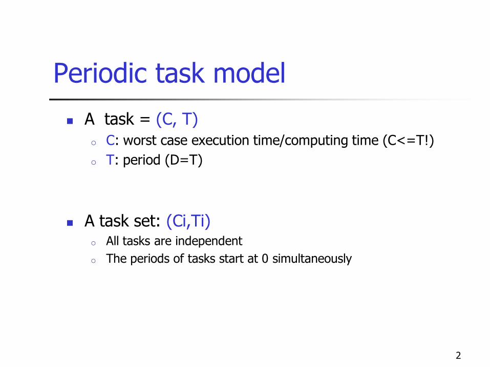
Periodic task model

A task = (C, T)

o C: worst case execution time/computing time (C<=T!)

o T: period (D=T)

A task set: (Ci,Ti)o All tasks are independent

o The periods of tasks start at 0 simultaneously

3

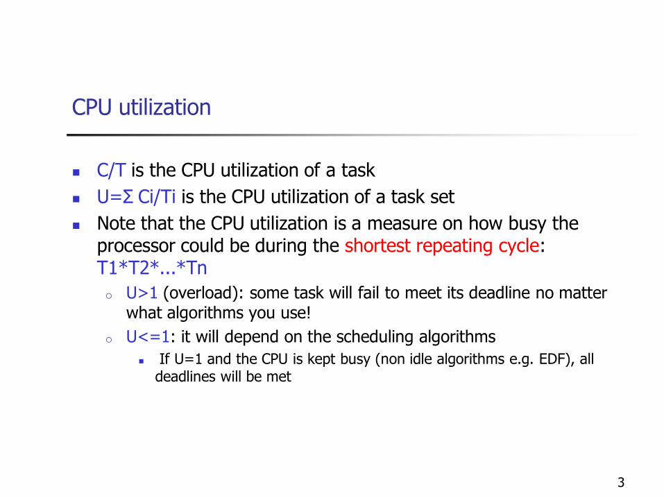
CPU utilization

C/T is the CPU utilization of a task

U=Σ Ci/Ti is the CPU utilization of a task set

Note that the CPU utilization is a measure on how busy the processor could be during the shortest repeating cycle: T1*T2*...*Tn

o U>1 (overload): some task will fail to meet its deadline no matter what algorithms you use!

o U<=1: it will depend on the scheduling algorithms

If U=1 and the CPU is kept busy (non idle algorithms e.g. EDF), all deadlines will be met

4

Scheduling Algorithms

Static Cyclic Scheduling (SCS)

Earliest Deadline First (EDF)

Rate Monotonic Scheduling (RMS)

Deadline Monotonic Scheduling (DMS)

5

Static cyclic scheduling

Shortest repeating cycle = least common multiple (LCM)

Within the cycle, it is possible to construct a static schedule i.e. a time table

Schedule task instances according to the time table within each cycle

Synchronous programming languages: Esterel, Lustre, Signal

6

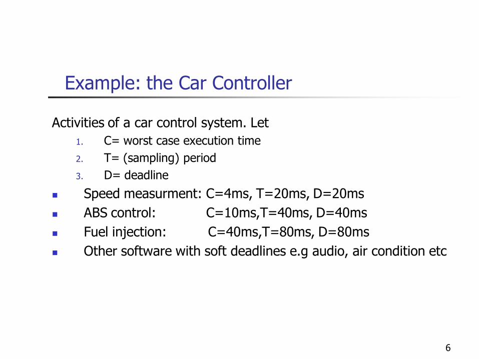
Example: the Car Controller

Activities of a car control system. Let

1. C= worst case execution time

2. T= (sampling) period

3. D= deadline

Speed measurment: C=4ms, T=20ms, D=20ms

ABS control: C=10ms,T=40ms, D=40ms

Fuel injection: C=40ms,T=80ms, D=80ms

Other software with soft deadlines e.g audio, air condition etc

7

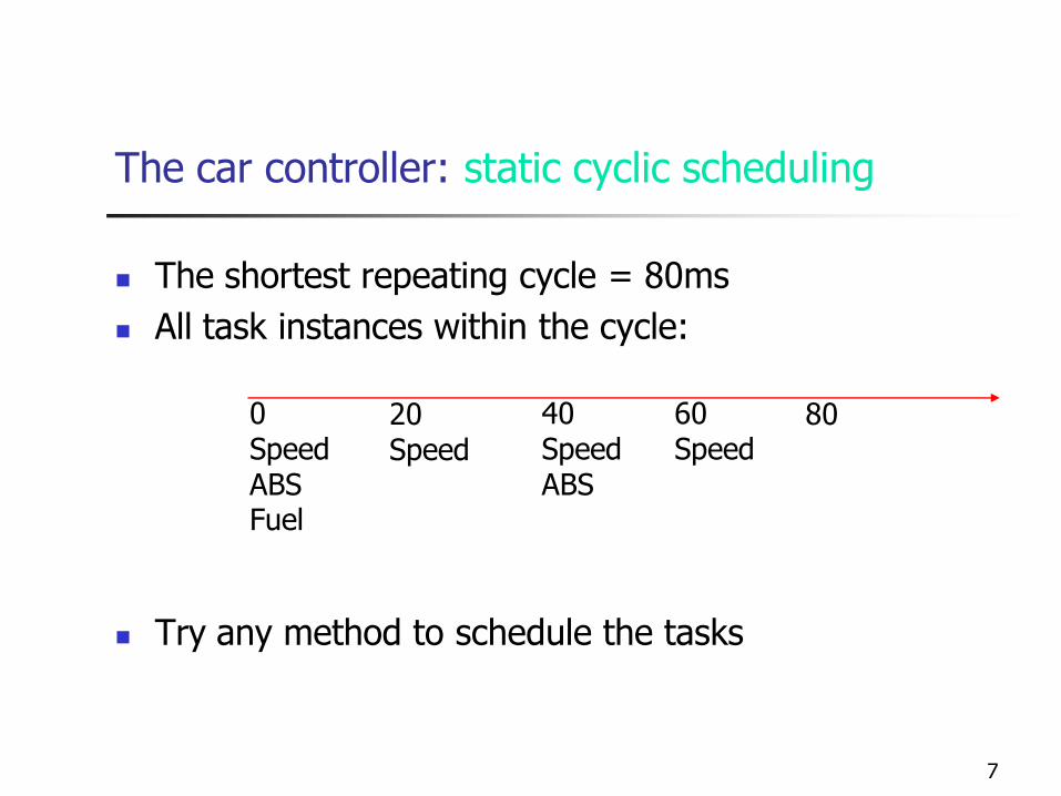
The car controller: static cyclic scheduling

The shortest repeating cycle = 80ms

All task instances within the cycle:

Try any method to schedule the tasks

0SpeedABSFuel

8040SpeedABS

20Speed

60Speed

8

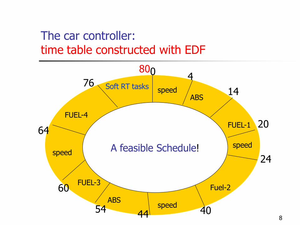
The car controller: time table constructed with EDF

A feasible Schedule!

04

14

20

404454

60

64

76speed

ABS

speed

Fuel-2

speedABS

FUEL-3

FUEL-1

speed

FUEL-4

Soft RT tasks

24

80

9

Static cyclic scheduling: + and –

Deterministic: predictable (+)

Easy to implement (+)

Inflexible (-)

o Difficult to modify, e.g adding another task

o Difficult to handle external events

The table can be huge (-)

o Huge memory-usage

o Difficult to construct the time table

10

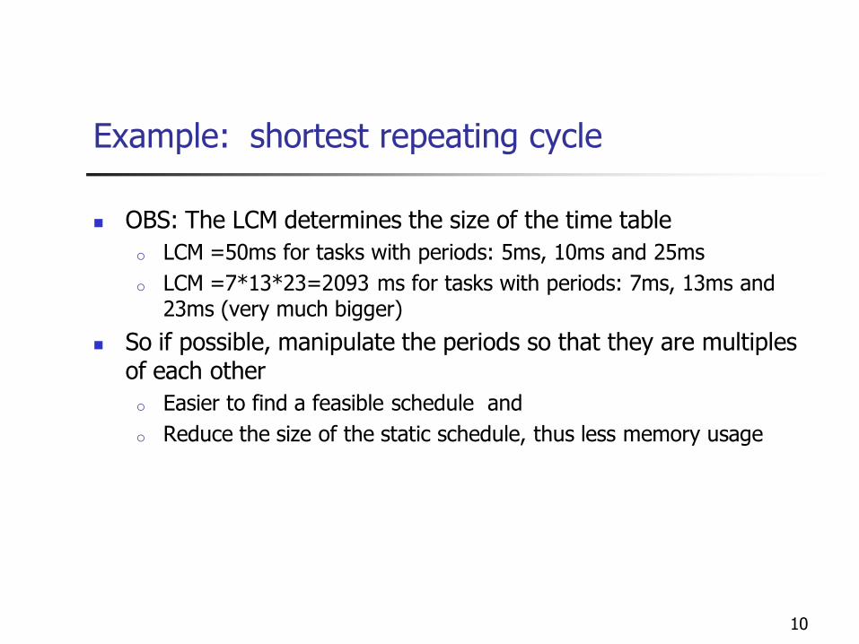
Example: shortest repeating cycle

OBS: The LCM determines the size of the time table

o LCM =50ms for tasks with periods: 5ms, 10ms and 25ms

o LCM =7*13*23=2093 ms for tasks with periods: 7ms, 13ms and 23ms (very much bigger)

So if possible, manipulate the periods so that they are multiples of each other

o Easier to find a feasible schedule and

o Reduce the size of the static schedule, thus less memory usage

11

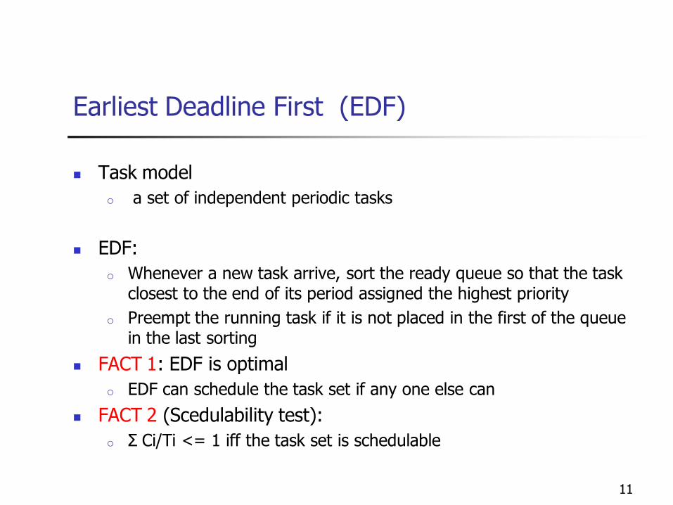
Earliest Deadline First (EDF)

Task model

o a set of independent periodic tasks

EDF:

o Whenever a new task arrive, sort the ready queue so that the task closest to the end of its period assigned the highest priority

o Preempt the running task if it is not placed in the first of the queue in the last sorting

FACT 1: EDF is optimal

o EDF can schedule the task set if any one else can

FACT 2 (Scedulability test):

o Σ Ci/Ti <= 1 iff the task set is schedulable

12

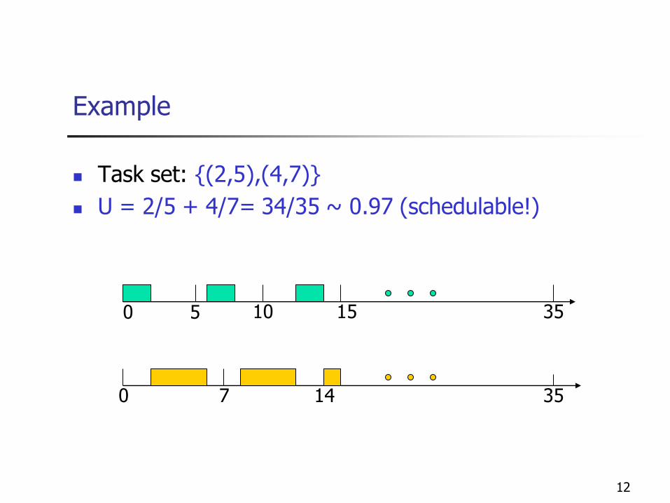
Example

Task set: {(2,5),(4,7)}

U = 2/5 + 4/7= 34/35 ~ 0.97 (schedulable!)

0 35

0 35

5 10

7 14

15

13

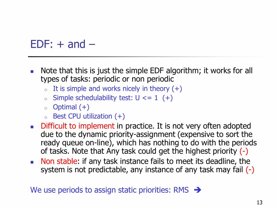
EDF: + and –

Note that this is just the simple EDF algorithm; it works for all types of tasks: periodic or non periodico It is simple and works nicely in theory (+)

o Simple schedulability test: U <= 1 (+)

o Optimal (+)

o Best CPU utilization (+)

Difficult to implement in practice. It is not very often adopted due to the dynamic priority-assignment (expensive to sort the ready queue on-line), which has nothing to do with the periods of tasks. Note that Any task could get the highest priority (-)

Non stable: if any task instance fails to meet its deadline, the system is not predictable, any instance of any task may fail (-)

We use periods to assign static priorities: RMS

Two classic papers on real-time systems

L. Sha, R. Rajkumar, and J. P. Lehoczky, Priority Inheritance Protocols: An Approach to Real-Time Synchronization. In IEEE Transactions on Computers, vol. 39, pp. 1175-1185, Sep. 1990. o Priority inversion and ceiling protocols

C. L. Liu , James W. Layland, Scheduling Algorithms for Multiprogramming in a Hard-Real-Time Environment, Journal of the ACM (JACM), v.20 n.1, p.46-61, Jan. 1973 o Rate monotonic scheduling

14

15

Rate Monotonic Scheduling: task model

Assume a set of periodic tasks: (Ci,Ti)

Di=Ti

Tasks are always released at the start of their periods

Tasks are independent

16

RMS: fixed/static-priority scheduling

Rate Monotonic Fixed-Priority Assignment:

o Tasks with smaller periods get higher priorities

Run-Time Scheduling:

o Preemptive highest priority first

FACT: RMS is optimal in the sense:

o If a task set is schedulable with any fixed-priorityscheduling algorithm, it is also schedulable with RMS

17

Example

20 202020

40

40 30

40

10 20

0 100 200 300

150 300

350

400

0

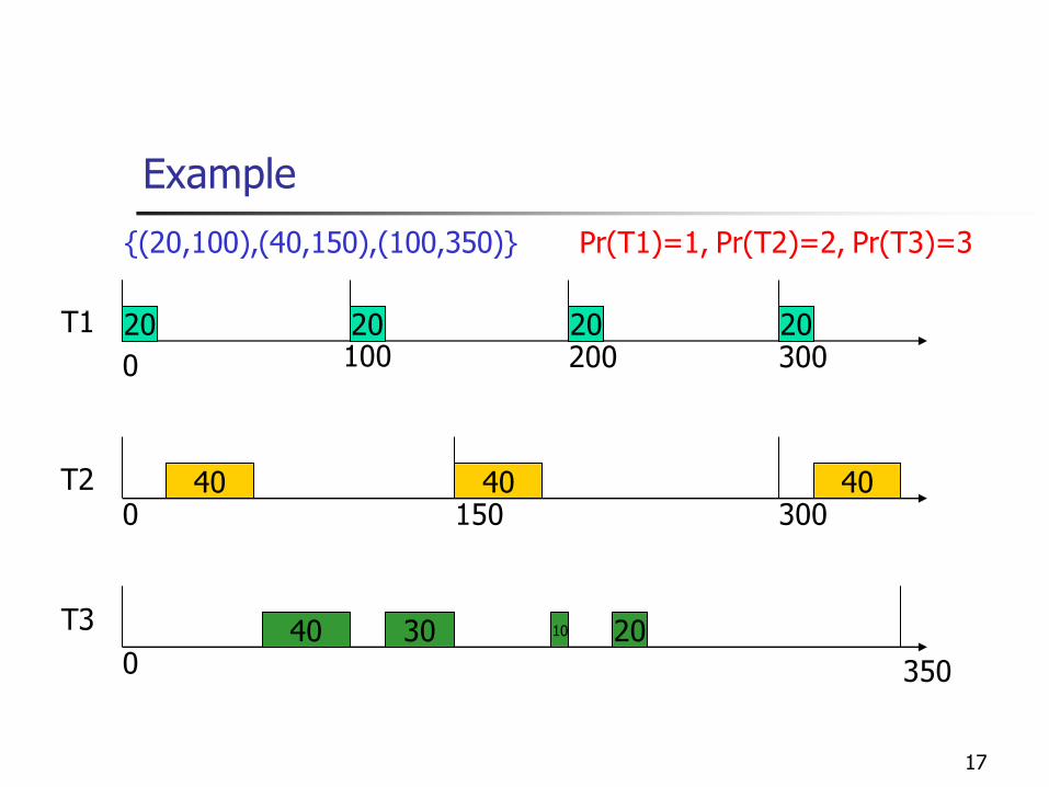
{(20,100),(40,150),(100,350)}

T1

T2

T3

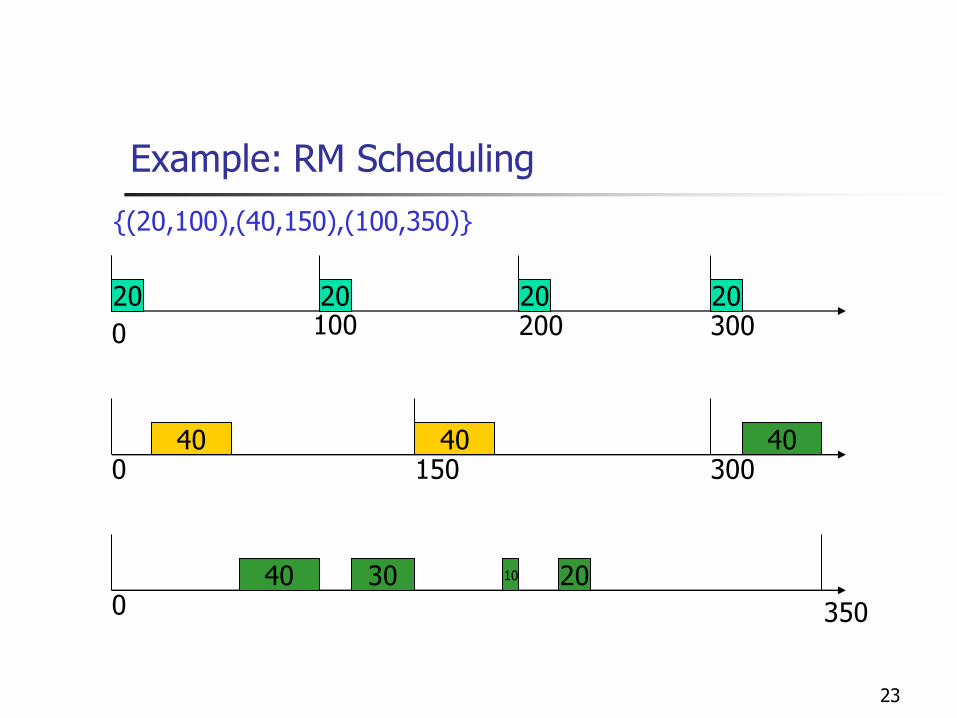
Pr(T1)=1, Pr(T2)=2, Pr(T3)=3

18

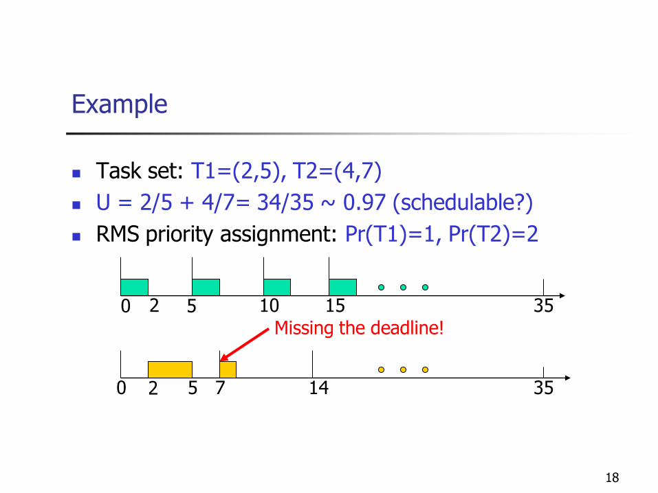
Example

Task set: T1=(2,5), T2=(4,7)

U = 2/5 + 4/7= 34/35 ~ 0.97 (schedulable?)

RMS priority assignment: Pr(T1)=1, Pr(T2)=2

0 35

0 35

5 10

7 14

15

2 5

2Missing the deadline!

19

RMS: schedulability test

U<1 doesn’t imply ’schedulable’ with RMSo OBS: the previous example is schedulable by EDF, not RMS

Idea: utilization boundo Given a task set S, find X(S) such that U<= X(S) if and only

if S is schedulable by RMS (necessary and sufficient test)

o Note that the bound X(S) for EDF is 1

20

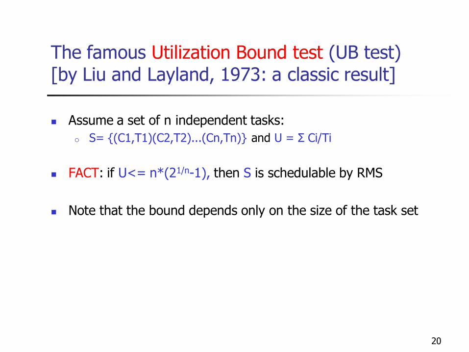
The famous Utilization Bound test (UB test)[by Liu and Layland, 1973: a classic result]

Assume a set of n independent tasks:

o S= {(C1,T1)(C2,T2)...(Cn,Tn)} and U = Σ Ci/Ti

FACT: if U<= n*(21/n-1), then S is schedulable by RMS

Note that the bound depends only on the size of the task set

21

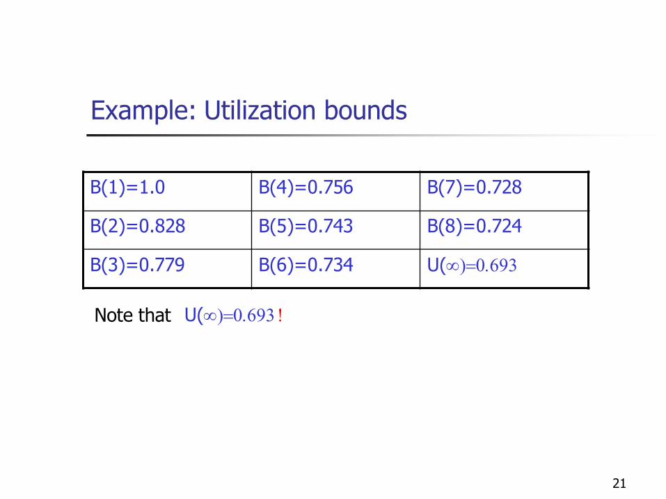
Example: Utilization bounds

B(1)=1.0 B(4)=0.756 B(7)=0.728

B(2)=0.828 B(5)=0.743 B(8)=0.724

B(3)=0.779 B(6)=0.734 U()=0.693

Note that U()=0.693 !

22

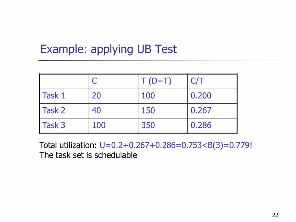
Example: applying UB Test

C T (D=T) C/T

Task 1 20 100 0.200

Task 2 40 150 0.267

Task 3 100 350 0.286

Total utilization: U=0.2+0.267+0.286=0.753<B(3)=0.779!The task set is schedulable

23

Example: RM Scheduling

20 202020

40

40 30

40

10 20

0 100 200 300

150 300

350

400

0

{(20,100),(40,150),(100,350)}

24

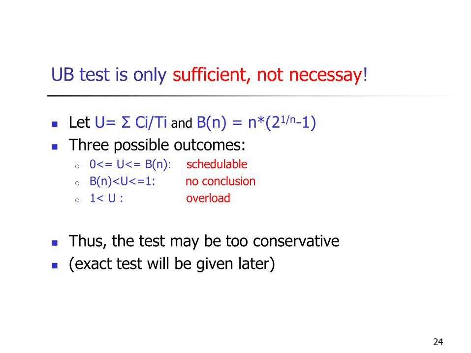
UB test is only sufficient, not necessay!

Let U= Σ Ci/Ti and B(n) = n*(21/n-1)

Three possible outcomes:o 0<= U<= B(n): schedulable

o B(n)<U<=1: no conclusion

o 1< U : overload

Thus, the test may be too conservative

(exact test will be given later)

25

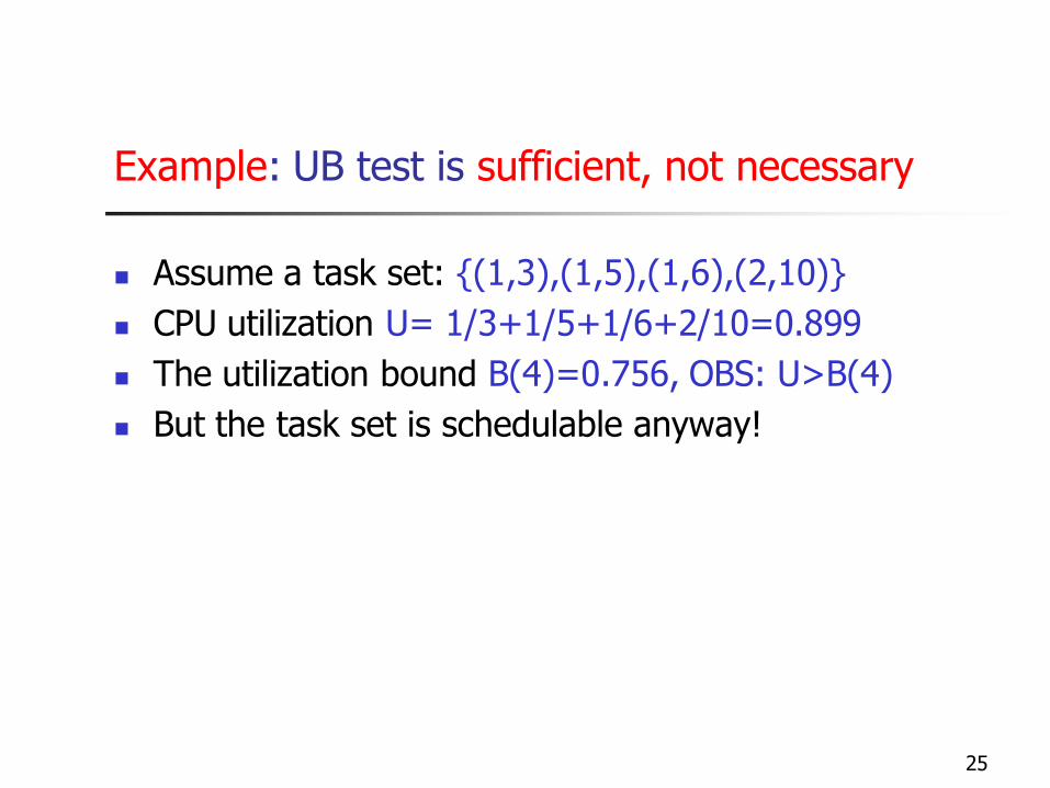
Example: UB test is sufficient, not necessary

Assume a task set: {(1,3),(1,5),(1,6),(2,10)}

CPU utilization U= 1/3+1/5+1/6+2/10=0.899

The utilization bound B(4)=0.756, OBS: U>B(4)

But the task set is schedulable anyway!

26

How to deal with tasks with the same period

What should we do if tasks have the same period?

Should we assign the same priority to the tasks?

How about the UB test? Is it still sufficient?

What happens at run time?

27

RMS: Summary

Task model:

o priodic, independent, D=T, and a task= (Ci,Ti)

Fixed-priority assignment:

o smaller periods = higher priorities

Run time scheduling: Preemptive HPF

Sufficient schedulability test: U<= n*(21/n-1)

Precise/exact schedulability test exists

28

RMS: + and –

Simple to understand (and remember!) (+)

Easy to implement (static/fixed priority assignment)(+)

Stable: though some of the lower priority tasks fail to meet deadlines, others may meet deadlines (+)

”lower” CPU utilization (-)

Requires D=T (-)

Only deal with independent tasks (-)

Non-precise schedulability analysis (-)

But these are not really disadvantages;they can be fixed (+++)

o We can solve all these problems except “lower” utilization

29

Critical instant: an important observation

Critical instant of a task is the time point at which the release of the task will yield the largest response time. It occurs when the task is released simultaneously with higher priority tasks

Note that the start of a task period is not necessarily at zero, or at the same time as the other tasks.

30

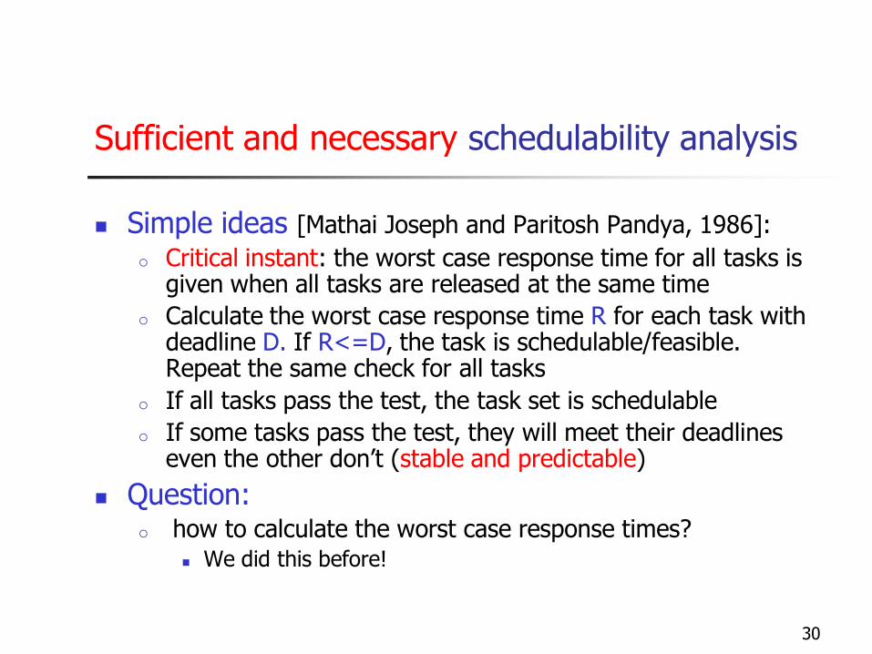
Sufficient and necessary schedulability analysis

Simple ideas [Mathai Joseph and Paritosh Pandya, 1986]:

o Critical instant: the worst case response time for all tasks is given when all tasks are released at the same time

o Calculate the worst case response time R for each task with deadline D. If R<=D, the task is schedulable/feasible. Repeat the same check for all tasks

o If all tasks pass the test, the task set is schedulable

o If some tasks pass the test, they will meet their deadlines even the other don’t (stable and predictable)

Question:o how to calculate the worst case response times?

We did this before!

31

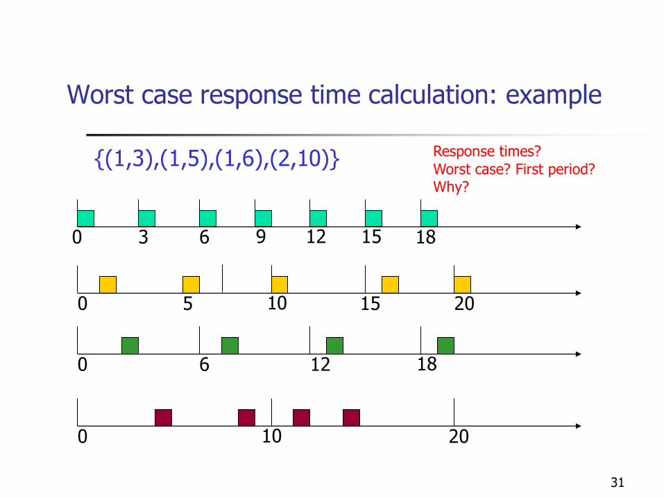
Worst case response time calculation: example

{(1,3),(1,5),(1,6),(2,10)}

0 3 6 9 12 15 18

5 10 15 200

0 6 12 18

0 10 20

Response times?

Worst case? First period?Why?

32

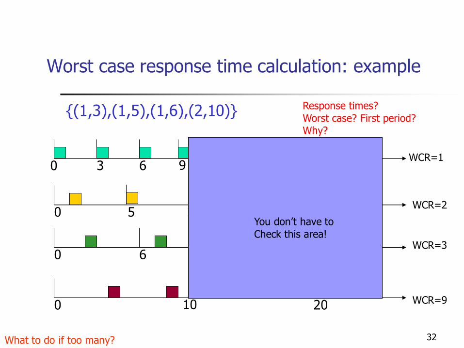
Worst case response time calculation: example

{(1,3),(1,5),(1,6),(2,10)}

0 3 6 9 12 15 18

5 10 15 200

0 6 12 18

0 10 20

Response times?

Worst case? First period?Why?

WCR=1

WCR=2

WCR=3

WCR=9

What to do if too many?

You don’t have to

Check this area!

33

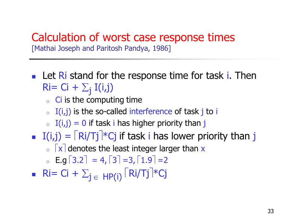
Calculation of worst case response times[Mathai Joseph and Paritosh Pandya, 1986]

Let Ri stand for the response time for task i. Then Ri= Ci + j I(i,j)

o Ci is the computing time

o I(i,j) is the so-called interference of task j to i

o I(i,j) = 0 if task i has higher priority than j

I(i,j) = Ri/Tj*Cj if task i has lower priority than j

o x denotes the least integer larger than x

o E.g 3.2 = 4, 3 =3, 1.9 =2

Ri= Ci + j HP(i) Ri/Tj*Cj

34

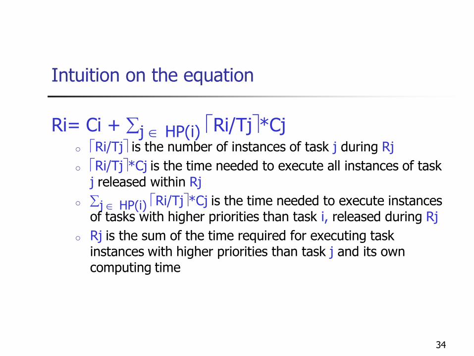
Intuition on the equation

Ri= Ci + j HP(i) Ri/Tj*Cjo Ri/Tj is the number of instances of task j during Rj

o Ri/Tj*Cj is the time needed to execute all instances of taskj released within Rj

o j HP(i) Ri/Tj*Cj is the time needed to execute instances of tasks with higher priorities than task i, released during Rj

o Rj is the sum of the time required for executing task instances with higher priorities than task j and its own computing time

35

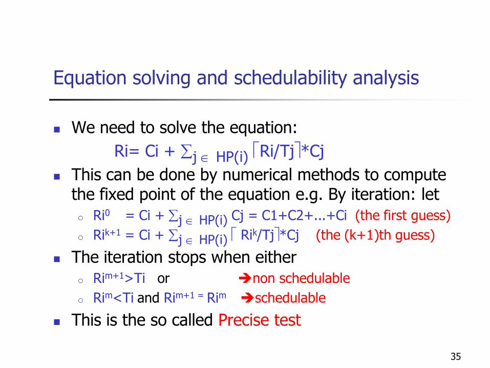
Equation solving and schedulability analysis

We need to solve the equation:

Ri= Ci + j HP(i) Ri/Tj*Cj

This can be done by numerical methods to compute the fixed point of the equation e.g. By iteration: let

o Ri0 = Ci + j HP(i) Cj = C1+C2+...+Ci (the first guess)

o Rik+1 = Ci + j HP(i) Rik/Tj*Cj (the (k+1)th guess)

The iteration stops when either

o Rim+1>Ti or non schedulable

o Rim<Ti and Rim+1 = Rim schedulable

This is the so called Precise test

36

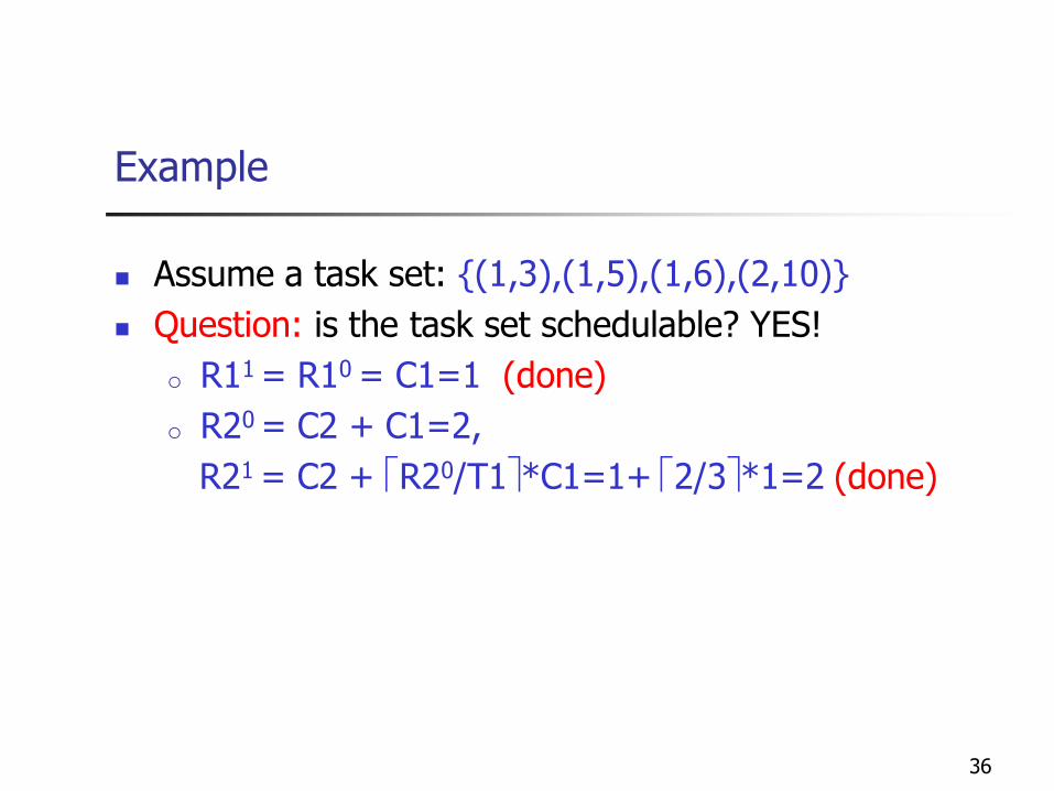
Example

Assume a task set: {(1,3),(1,5),(1,6),(2,10)}

Question: is the task set schedulable? YES!

o R11 = R10 = C1=1 (done)

o R20 = C2 + C1=2,

R21 = C2 + R20/T1*C1=1+ 2/3*1=2 (done)

37

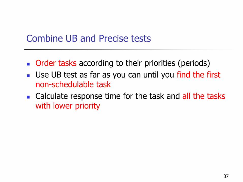
Combine UB and Precise tests

Order tasks according to their priorities (periods)

Use UB test as far as you can until you find the first non-schedulable task

Calculate response time for the task and all the tasks with lower priority

38

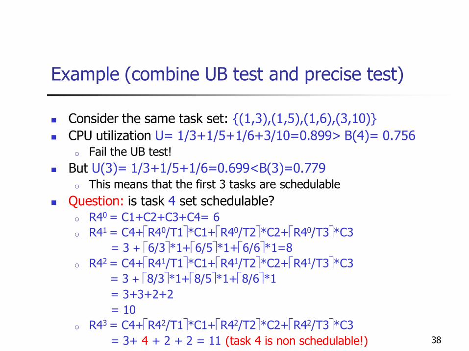
Example (combine UB test and precise test)

Consider the same task set: {(1,3),(1,5),(1,6),(3,10)}

CPU utilization U= 1/3+1/5+1/6+3/10=0.899> B(4)= 0.756o Fail the UB test!

But U(3)= 1/3+1/5+1/6=0.699<B(3)=0.779o This means that the first 3 tasks are schedulable

Question: is task 4 set schedulable?o R40 = C1+C2+C3+C4= 6

o R41 = C4+R40/T1*C1+R40/T2*C2+R40/T3*C3

= 3 + 6/3*1+6/5*1+6/6*1=8

o R42 = C4+R41/T1*C1+R41/T2*C2+R41/T3*C3

= 3 + 8/3*1+8/5*1+8/6*1

= 3+3+2+2

= 10

o R43 = C4+R42/T1*C1+R42/T2*C2+R42/T3*C3

= 3+ 4 + 2 + 2 = 11 (task 4 is non schedulable!)

39

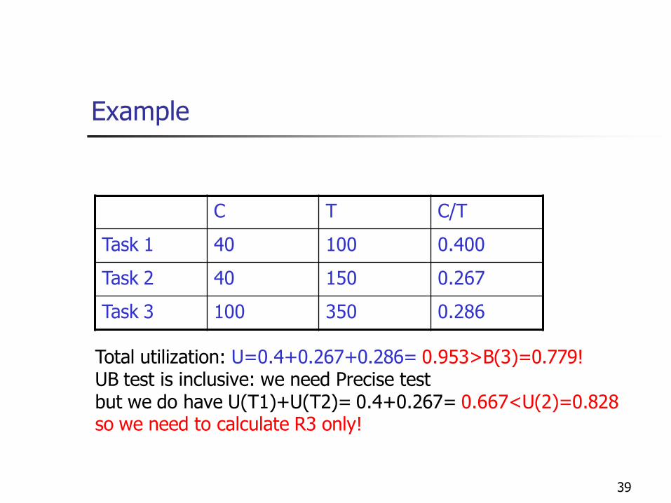
Example

C T C/T

Task 1 40 100 0.400

Task 2 40 150 0.267

Task 3 100 350 0.286

Total utilization: U=0.4+0.267+0.286= 0.953>B(3)=0.779!UB test is inclusive: we need Precise testbut we do have U(T1)+U(T2)= 0.4+0.267= 0.667<U(2)=0.828so we need to calculate R3 only!

40

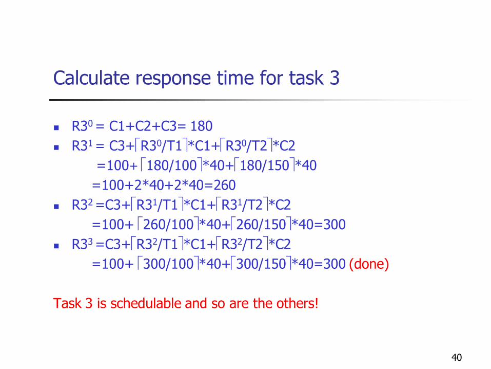
Calculate response time for task 3

R30 = C1+C2+C3= 180

R31 = C3+R30/T1*C1+R30/T2*C2

=100+ 180/100*40+180/150*40

=100+2*40+2*40=260

R32 =C3+R31/T1*C1+R31/T2*C2

=100+ 260/100*40+260/150*40=300

R33 =C3+R32/T1*C1+R32/T2*C2

=100+ 300/100*40+300/150*40=300 (done)

Task 3 is schedulable and so are the others!

41

Question: other priority-assignments

Could we calculate the response times by the same equation for different priority assignment?

42

Precedence constraints

How to handle precedence constraints?

We can always try the ’old’ method: static cyclic scheduling!

Alternatively, take the precedence constraints (DAG) into account in priority assignment: the priority-ordering must satisfy the precedence constraints

o Precise schedulability test is valid: use the same method as beforee to calculate the response times.

43

Summary: Three ways to check schedulability

1. UB test (simple but conservative)

2. Response time calculation (precise test)

3. Construct a schedule for the first periods

o assume the first instances arrive at time 0 (critical instant)

o draw the schedule for the first periods

o if all tasks are finished before the end of the first periods, schedulable, otherwise NO

44

Extensions to the basic RMS

Deadline <= Period

Interrupt handling

Non zero OH for context switch

Non preemptive sections

Resource Sharing

45

RMS for tasks with D <= T

RMS is no longer optimal (example?)

Utilization bound test must be modified

Response time test is still applicable

o Assuming that fixed-priority assignment is adopted

o But considering the critical instant and checking the first deadlines principle are still applicable

46

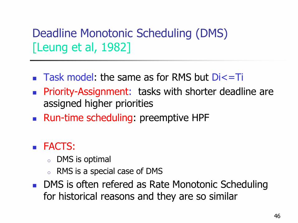
Deadline Monotonic Scheduling (DMS) [Leung et al, 1982]

Task model: the same as for RMS but Di<=Ti

Priority-Assignment: tasks with shorter deadline are assigned higher priorities

Run-time scheduling: preemptive HPF

FACTS:

o DMS is optimal

o RMS is a special case of DMS

DMS is often refered as Rate Monotonic Scheduling for historical reasons and they are so similar

47

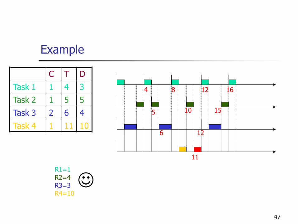
Example

C T D

Task 1 1 4 3

Task 2 1 5 5

Task 3 2 6 4

Task 4 1 11 10

4 8 12 16

5 10 15

6 12

11

R1=1

R2=4R3=3R4=10

48

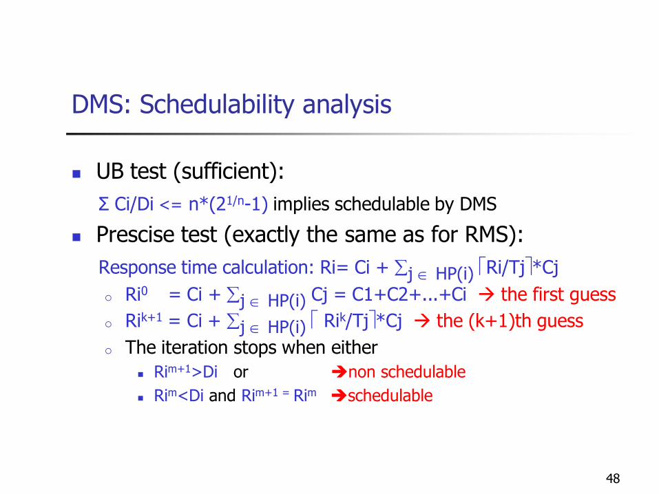
DMS: Schedulability analysis

UB test (sufficient):

Σ Ci/Di <= n*(21/n-1) implies schedulable by DMS

Prescise test (exactly the same as for RMS):

Response time calculation: Ri= Ci + j HP(i) Ri/Tj*Cj

o Ri0 = Ci + j HP(i) Cj = C1+C2+...+Ci the first guess

o Rik+1 = Ci + j HP(i) Rik/Tj*Cj the (k+1)th guess

o The iteration stops when either

Rim+1>Di or non schedulable

Rim<Di and Rim+1 = Rim schedulable

49

Summary: 3 ways for DMS schedulability check

UB test (sufficient, inconclusive)

Response time calculation

Draw the schedule for the first periods

50

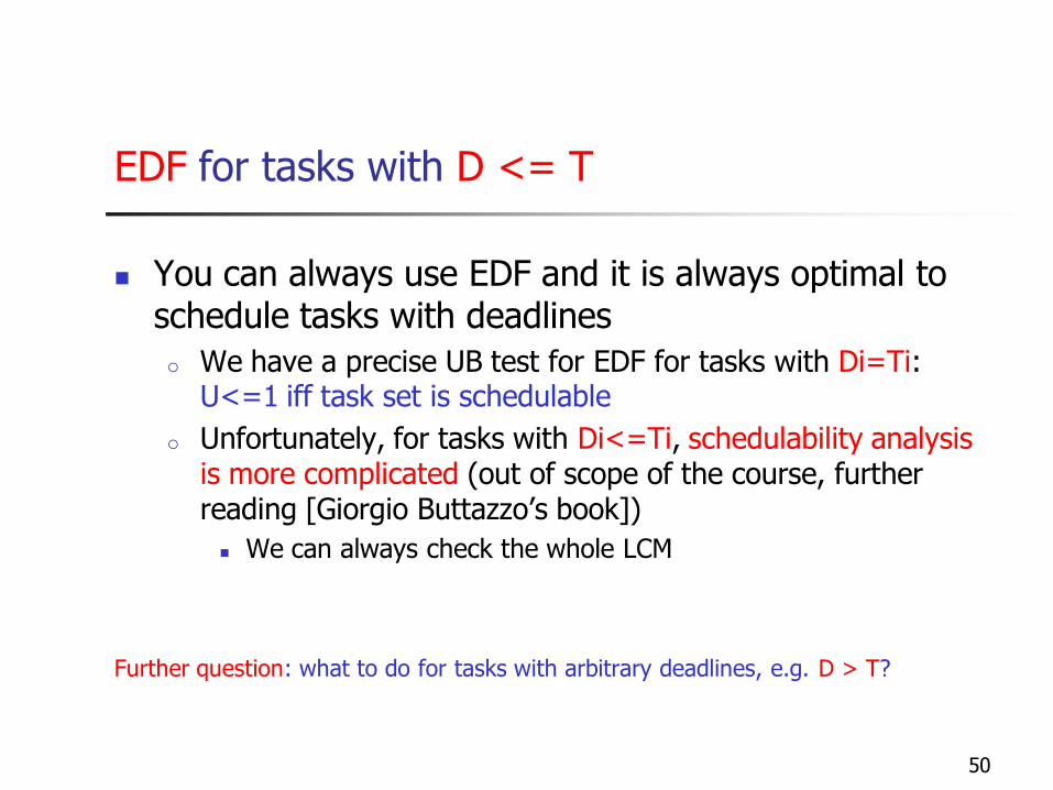
EDF for tasks with D <= T

You can always use EDF and it is always optimal to schedule tasks with deadlines

o We have a precise UB test for EDF for tasks with Di=Ti: U<=1 iff task set is schedulable

o Unfortunately, for tasks with Di<=Ti, schedulability analysisis more complicated (out of scope of the course, further reading [Giorgio Buttazzo’s book])

We can always check the whole LCM

Further question: what to do for tasks with arbitrary deadlines, e.g. D > T?

51

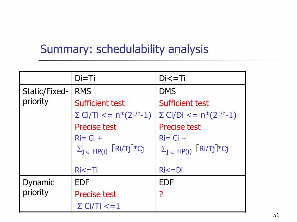
Summary: schedulability analysis

Di=Ti Di<=Ti

Static/Fixed-priority

RMS

Sufficient test

Σ Ci/Ti <= n*(21/n-1)

Precise test

Ri= Ci +

j HP(i) Ri/Tj*Cj

Ri<=Ti

DMS

Sufficient test

Σ Ci/Di <= n*(21/n-1)

Precise test

Ri= Ci +

j HP(i) Ri/Tj*Cj

Ri<=Di

Dynamic priority

EDF

Precise test

Σ Ci/Ti <=1

EDF

?

52

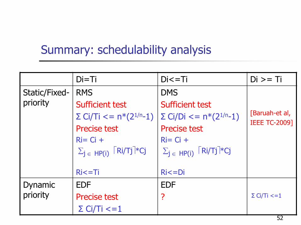
Summary: schedulability analysis

Di=Ti Di<=Ti Di >= Ti

Static/Fixed-priority

RMS

Sufficient test

Σ Ci/Ti <= n*(21/n-1)

Precise test

Ri= Ci +

j HP(i) Ri/Tj*Cj

Ri<=Ti

DMS

Sufficient test

Σ Ci/Di <= n*(21/n-1)

Precise test

Ri= Ci +

j HP(i) Ri/Tj*Cj

Ri<=Di

[Baruah-et al,

IEEE TC-2009]

Dynamic priority

EDF

Precise test

Σ Ci/Ti <=1

EDF

? Σ Ci/Ti <=1

53

Extensions to the basic RMS

Deadline <= Period

Interrupt handling

Non zero OH for context switch

Non preemptive sections

Resource Sharing

54

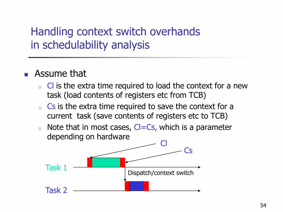
Handling context switch overhandsin schedulability analysis

Assume that

o Cl is the extra time required to load the context for a new task (load contents of registers etc from TCB)

o Cs is the extra time required to save the context for a current task (save contents of registers etc to TCB)

o Note that in most cases, Cl=Cs, which is a parameterdepending on hardware

Task 1

Task 2

Dispatch/context switch

ClCs

55

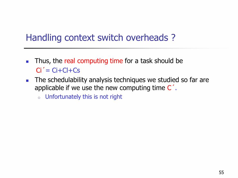
Handling context switch overheads ?

Thus, the real computing time for a task should be

Ci´= Ci+Cl+Cs

The schedulability analysis techniques we studied so far are applicable if we use the new computing time C´.

o Unfortunately this is not right

56

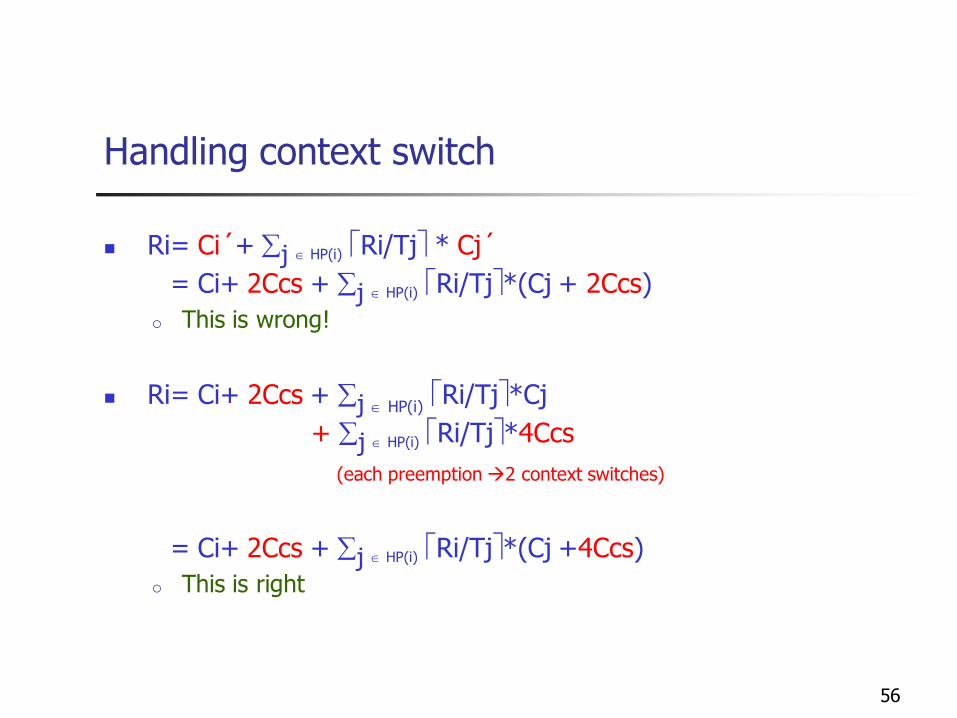
Handling context switch

Ri= Ci´+ j HP(i) Ri/Tj * Cj´

= Ci+ 2Ccs + j HP(i) Ri/Tj*(Cj + 2Ccs)

o This is wrong!

Ri= Ci+ 2Ccs + j HP(i)Ri/Tj*Cj

+ j HP(i) Ri/Tj*4Ccs

(each preemption 2 context switches)

= Ci+ 2Ccs + j HP(i) Ri/Tj*(Cj +4Ccs)

o This is right

57

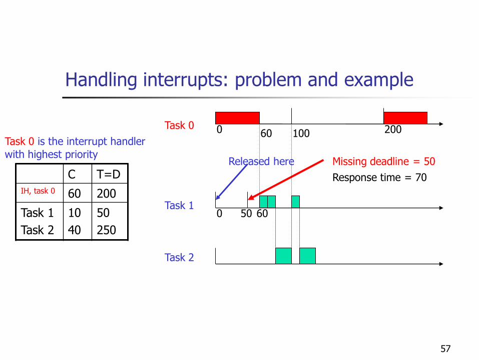
Handling interrupts: problem and example

C T=D

IH, task 0 60 200

Task 1

Task 2

10

40

50

250

Task 0 is the interrupt handler

with highest priority

Task 0

Task 1

0 100 20060

50

Missing deadline = 50Released here

0 60

Response time = 70

Task 2

58

Handling interrupts: solution

Whenever possible: move code from the interrupt handler to a special application task with the same rate as the interrupt handler to make the interrupt handler (with high priority) as shorter as possible

Interrupt processing can be inconsistent with RM priority assignment, and therefore can effect schedulability of task set (previous example)o Interrupt handler runs with high priority despites its period

o Interrupt processing may delay tasks with shorter periods (deadlines)

o how to calculate the worst case response time ?

59

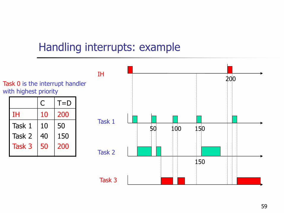
Handling interrupts: example

C T=D

IH 10 200

Task 1

Task 2

Task 3

10

40

50

50

150

200

Task 0 is the interrupt handler

with highest priority

IH

Task 1

200

50

Task 2

100 150

150

Task 3

60

Handling non-preemtive sections

So far, we have assumed that all tasks are preemptive regions of code. This not always the case e.g code for context switch though it may be short, and the short part of the interrupt handler as we considered before

o Some section of a task is non preemptive

In general, we may assume an extra parameter B in the task model, which is the computing time for the non preemtive section of a task.

o Bi = computing time of non preemptive section of task i

61

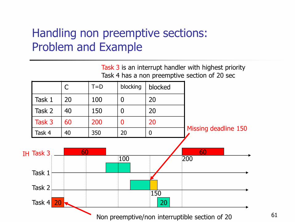
Handling non preemptive sections:Problem and Example

C T=D blocking blocked

Task 1 20 100 0 20

Task 2 40 150 0 20

Task 3 60 200 0 20

Task 4 40 350 20 0

20

100 200

150

Task 3

Task 1

Task 2

Task 4

IH

20

Missing deadline 150

Task 3 is an interrupt handler with highest priority

Task 4 has a non preemptive section of 20 sec

60 60

Non preemptive/non interruptible section of 20

62

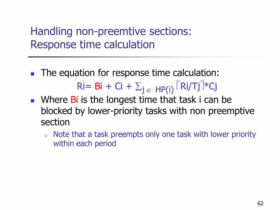
Handling non-preemtive sections:Response time calculation

The equation for response time calculation:

Ri= Bi + Ci + j HP(i) Ri/Tj*Cj

Where Bi is the longest time that task i can be blocked by lower-priority tasks with non preemptive section

o Note that a task preempts only one task with lower priority within each period

63

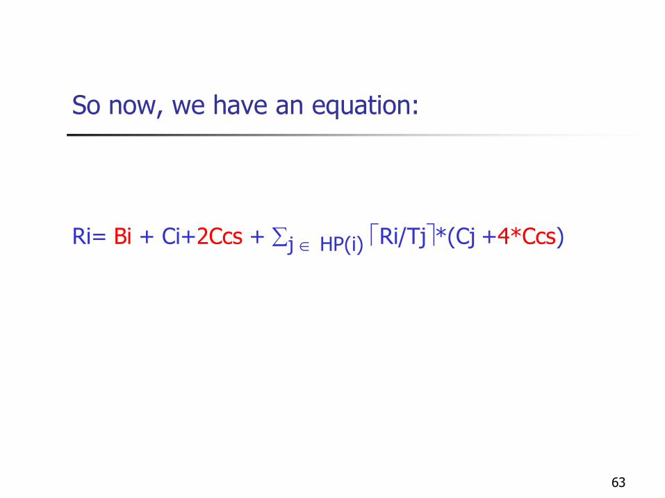
So now, we have an equation:

Ri= Bi + Ci+2Ccs + j HP(i) Ri/Tj*(Cj +4*Ccs)

64

The Jitter Problem

So far, we have assumed that tasks are released at a constant rate (at the start of a constant period)

This is true in practice and a realistic assumption

However, there are situations where the period or rather the release time may ’jitter’ or change a little, but the jitter is bounded with some constant J

The jitter may cause some task missing deadline

65

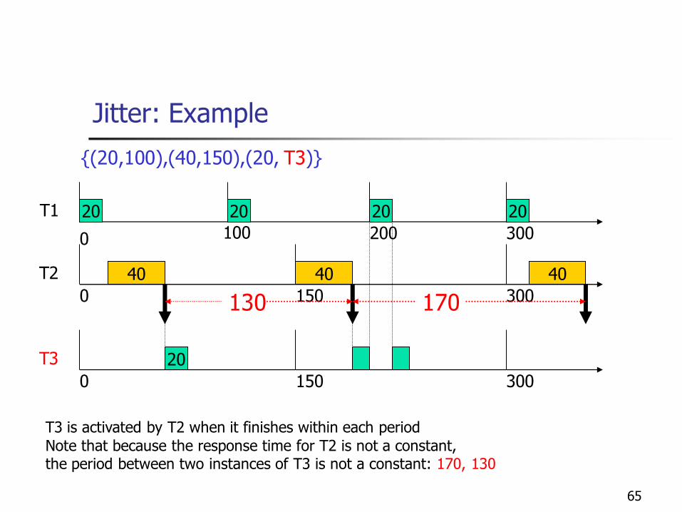
Jitter: Example

20 202020

40 40

0 100 200 300

150 300

40

0

{(20,100),(40,150),(20, T3)}

T1

T2

150 3000

T3

130 170

T3 is activated by T2 when it finishes within each period

Note that because the response time for T2 is not a constant, the period between two instances of T3 is not a constant: 170, 130

20

66

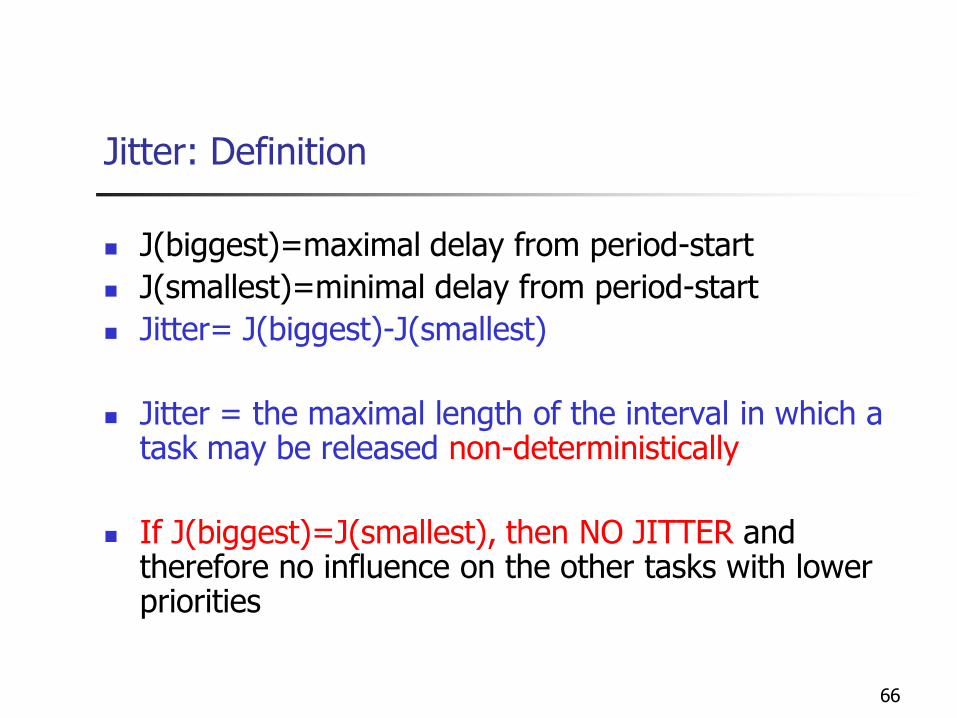
Jitter: Definition

J(biggest)=maximal delay from period-start

J(smallest)=minimal delay from period-start

Jitter= J(biggest)-J(smallest)

Jitter = the maximal length of the interval in which a task may be released non-deterministically

If J(biggest)=J(smallest), then NO JITTER and therefore no influence on the other tasks with lower priorities

67

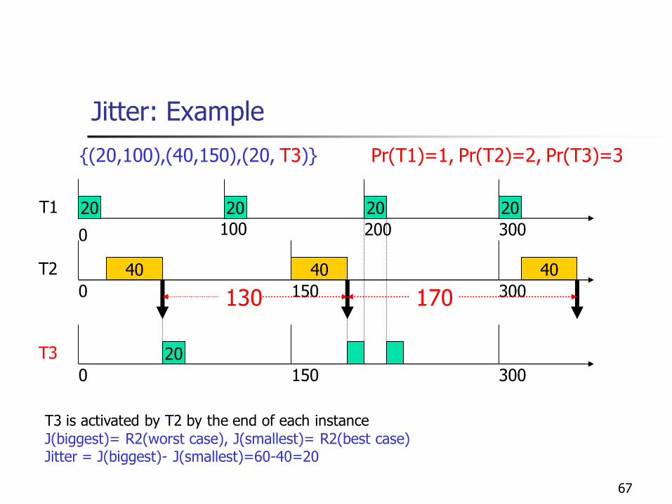
Jitter: Example

20 202020

40 40

0 100 200 300

150 300

40

0

{(20,100),(40,150),(20, T3)}

T1

T2

Pr(T1)=1, Pr(T2)=2, Pr(T3)=3

150 3000

T3

130 170

T3 is activated by T2 by the end of each instance

J(biggest)= R2(worst case), J(smallest)= R2(best case)Jitter = J(biggest)- J(smallest)=60-40=20

20

68

Jitter: Example

20 202020

40 40

0 100 200 300

150 300

40

0

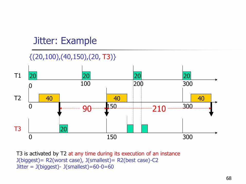
{(20,100),(40,150),(20, T3)}

T1

T2

150 3000

T3

90 210

T3 is activated by T2 at any time during its execution of an instance

J(biggest)= R2(worst case), J(smallest)= R2(best case)-C2Jitter = J(biggest)- J(smallest)=60-0=60

20

69

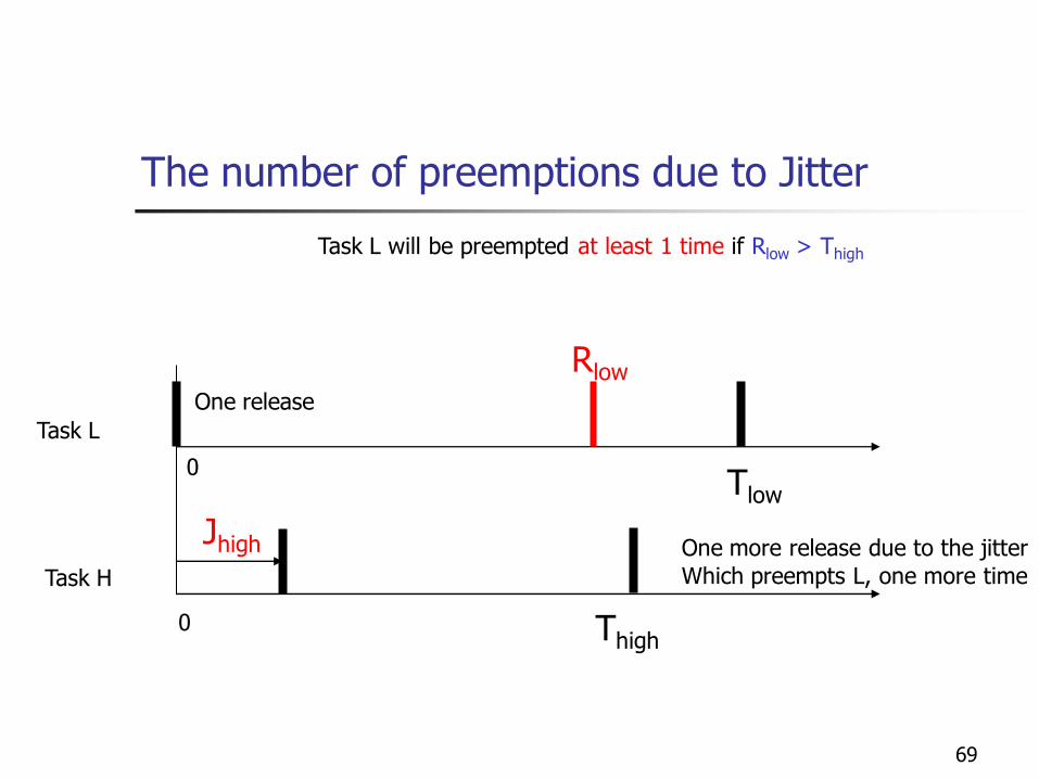
The number of preemptions due to Jitter

Task L

Task H

0

Tlow

Rlow

Thigh

Jhigh

0

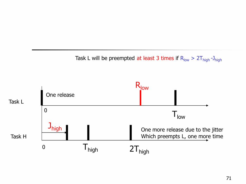
One release

One more release due to the jitter

Which preempts L, one more time

Task L will be preempted at least 1 time if Rlow > Thigh

70

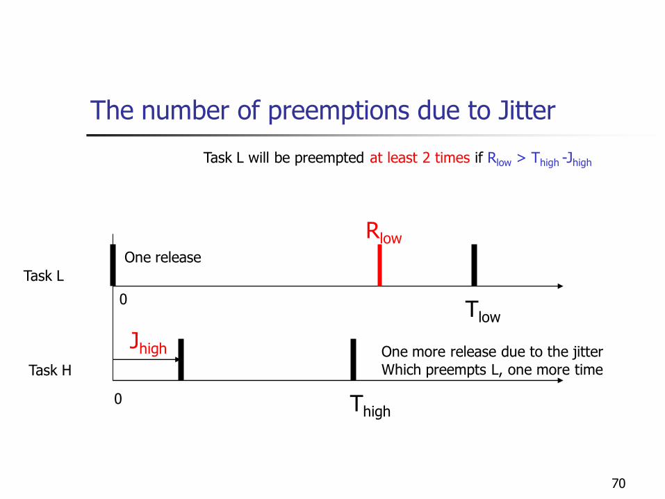
The number of preemptions due to Jitter

Task L

Task H

0

Tlow

Rlow

Thigh

Jhigh

0

One release

One more release due to the jitter

Which preempts L, one more time

Task L will be preempted at least 2 times if Rlow > Thigh -Jhigh

71

Task L

Task H

0

Tlow

Rlow

2Thigh

Jhigh

0

One release

One more release due to the jitter

Which preempts L, one more time

Task L will be preempted at least 3 times if Rlow > 2Thigh -Jhigh

Thigh

72

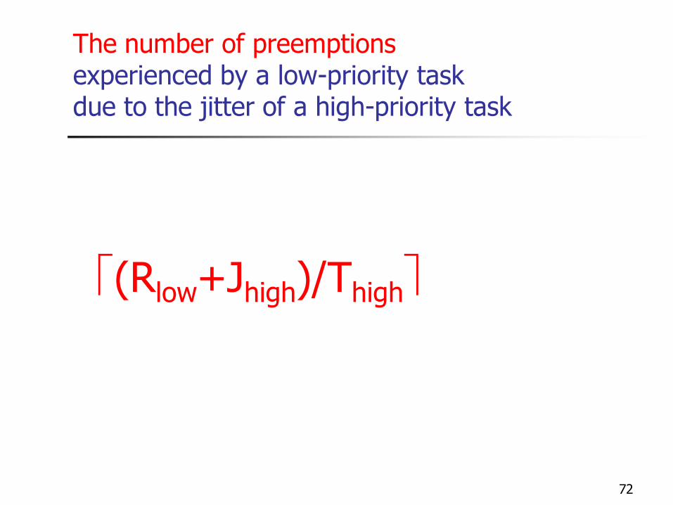
The number of preemptionsexperienced by a low-priority taskdue to the jitter of a high-priority task

(Rlow+Jhigh)/Thigh

73

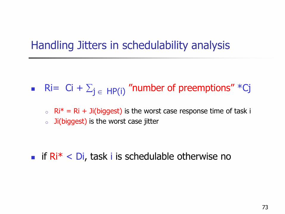
Handling Jitters in schedulability analysis

Ri= Ci + j HP(i) ”number of preemptions” *Cj

o Ri* = Ri + Ji(biggest) is the worst case response time of task i

o Ji(biggest) is the worst case jitter

if Ri* < Di, task i is schedulable otherwise no

74

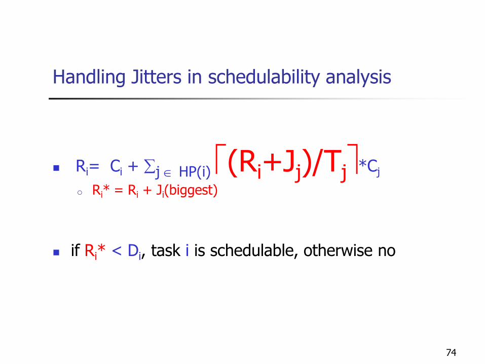
Handling Jitters in schedulability analysis

Ri= Ci + j HP(i) (Ri+Jj)/Tj*Cj

o Ri* = Ri + Ji(biggest)

if Ri* < Di, task i is schedulable, otherwise no

75

Now, we have an equation:

Ri= Ci+ 2Ccs + Bi + j HP(i) (Ri+Jj)/Tj*(Cj +4Ccs)

The response time for task i

Ri* = Ri+Ji(biggest)

Ji(biggest) is the ”biggest jitter” for task i

76

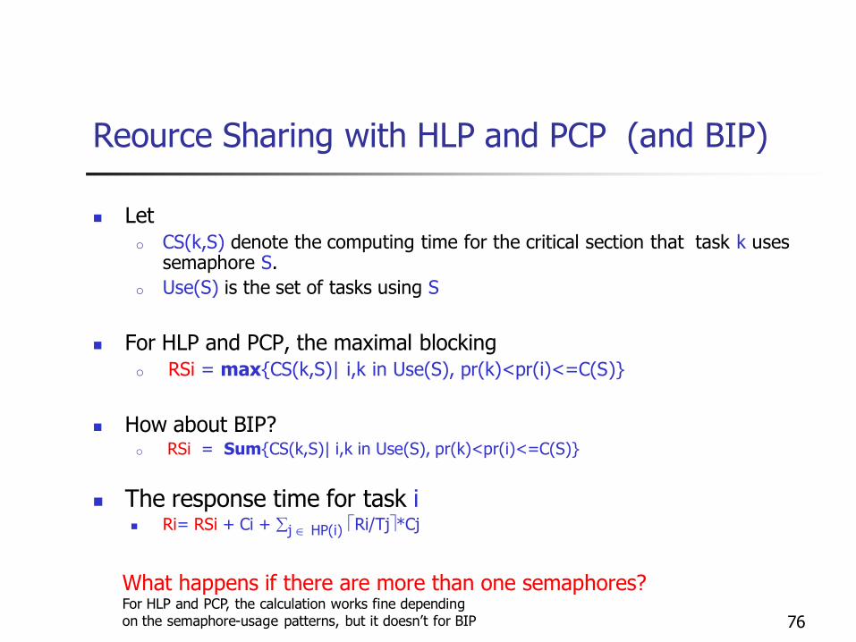
Reource Sharing with HLP and PCP (and BIP)

Let o CS(k,S) denote the computing time for the critical section that task k uses

semaphore S.

o Use(S) is the set of tasks using S

For HLP and PCP, the maximal blockingo RSi = max{CS(k,S)| i,k in Use(S), pr(k)<pr(i)<=C(S)}

How about BIP? o RSi = Sum{CS(k,S)| i,k in Use(S), pr(k)<pr(i)<=C(S)}

The response time for task i Ri= RSi + Ci + j HP(i) Ri/Tj*Cj

What happens if there are more than one semaphores?For HLP and PCP, the calculation works fine depending on the semaphore-usage patterns, but it doesn’t for BIP

77

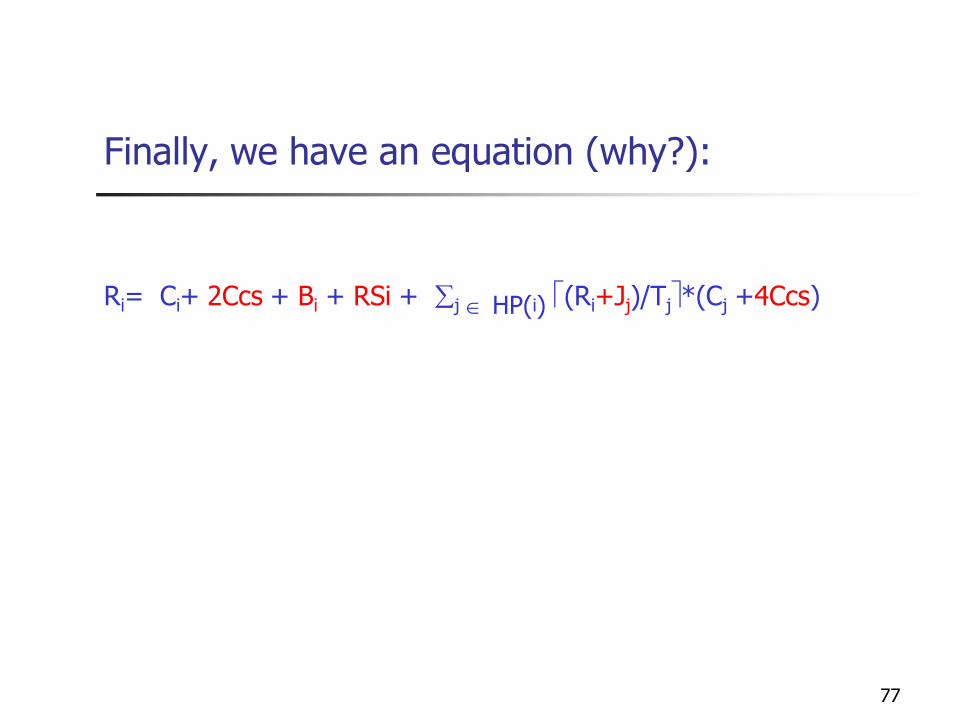
Finally, we have an equation (why?):

Ri= Ci+ 2Ccs + Bi + RSi + j HP(i) (Ri+Jj)/Tj*(Cj +4Ccs)

78

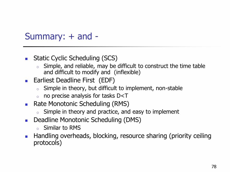
Summary: + and -

Static Cyclic Scheduling (SCS)o Simple, and reliable, may be difficult to construct the time table

and difficult to modify and (inflexible)

Earliest Deadline First (EDF)o Simple in theory, but difficult to implement, non-stable

o no precise analysis for tasks D<T

Rate Monotonic Scheduling (RMS)o Simple in theory and practice, and easy to implement

Deadline Monotonic Scheduling (DMS)o Similar to RMS

Handling overheads, blocking, resource sharing (priority ceiling protocols)