Scarred Eigenstates for Quantum Cat Maps of …faure/articles/scars_02.pdfScarred Eigenstates for...
44
Digital Object Identifier (DOI) 10.1007/s00220-003-0888-3 Commun. Math. Phys. 239, 449–492 (2003) Communications in Mathematical Physics Scarred Eigenstates for Quantum Cat Maps of Minimal Periods Fr´ ed´ eric Faure 1 , St´ ephane Nonnenmacher 2 , Stephan De Bi` evre 3 1 Laboratoire de Physique et Mod´ elisation des Milieux Condens´ es (LPM2C) (Maison des Magist` eres Jean Perrin, CNRS), BP 166, 38042 Grenoble C´ edex 9, France. E-mail: [email protected] 2 Service de Physique Th´ eorique, CEA/DSM/PhT Unit´ e de recherche associ´ ee au CNRS CEA/Saclay, 91191 Gif-sur-Yvette C´ edex, France. E-mail: [email protected] 3 UFR de Math.–UMRAGAT, Universit´ e des Sciences et Technologies de Lille, 59655 Villeneuve d’Ascq, France. E-mail: [email protected] Received: 5 August 2002 / Accepted: 21 February 2003 Published online: 2 July 2003 – © Springer-Verlag 2003 Abstract: In this paper we construct a sequence of eigenfunctions of the “quantum Arnold’s cat map” that, in the semiclassical limit, shows a strong scarring phenomenon on the periodic orbits of the dynamics. More precisely, those states have a semiclassical limit measure that is the sum of 1/2 the normalized Lebesgue measure on the torus plus 1/2 the normalized Dirac measure concentrated on any a priori given periodic orbit of the dynamics. It is known (the Schnirelman theorem) that “most” sequences of ei- genfunctions equidistribute on the torus. The sequences we construct therefore provide an example of an exception to this general rule. Our method of construction and proof exploits the existence of special values of for which the quantum period of the map is relatively “short”, and a sharp control on the evolution of coherent states up to this time scale. We also provide a pointwise description of these states in phase space, which uncovers their “hyperbolic” structure in the vicinity of the fixed points and yields more precise localization estimates. 1. Introduction One of the main problems in quantum chaos is the understanding of the semiclassical behaviour of the eigenfunctions of quantum dynamical systems having a chaotic clas- sical limit. The main theorem in this context is the Schnirelman theorem [Sc, CdV, Z1, HMR, BouDB]. It roughly states that “most” eigenfunctions equidistribute on the available phase space in the classical limit. This leaves open the question of the exis- tence of exceptional sequences of eigenfunctions with a different limit. In the case of “hard chaos” (uniformly hyperbolic systems), numerical computations have shown the presence of “scars” on certain eigenfunctions [He], i.e. a visual enhancement of the wavefunction on an unstable periodic orbit. Up to now all theories of this phenomenon have required some kind of averaging over a (semiclassically large) set of eigenfunctions [Bog, Ber, He, KH]. In addition, scarring is often described in the physics literature as a
Transcript of Scarred Eigenstates for Quantum Cat Maps of …faure/articles/scars_02.pdfScarred Eigenstates for...
Digital Object Identifier (DOI) 10.1007/s00220-003-0888-3Commun. Math. Phys. 239, 449–492 (2003) Communications in
MathematicalPhysics
Scarred Eigenstates for Quantum Cat Mapsof Minimal Periods
Frederic Faure1, Stephane Nonnenmacher2, Stephan De Bievre3
1 Laboratoire de Physique et Modelisation des Milieux Condenses (LPM2C) (Maison des MagisteresJean Perrin, CNRS), BP 166, 38042 Grenoble Cedex 9, France. E-mail: [email protected]
2 Service de Physique Theorique, CEA/DSM/PhT Unite de recherche associee au CNRS CEA/Saclay,91191 Gif-sur-Yvette Cedex, France. E-mail: [email protected]
3 UFR de Math.–UMR AGAT, Universite des Sciences et Technologies de Lille,59655 Villeneuve d’Ascq, France. E-mail: [email protected]
Received: 5 August 2002 / Accepted: 21 February 2003Published online: 2 July 2003 – © Springer-Verlag 2003
Abstract: In this paper we construct a sequence of eigenfunctions of the “quantumArnold’s cat map” that, in the semiclassical limit, shows a strong scarring phenomenonon the periodic orbits of the dynamics. More precisely, those states have a semiclassicallimit measure that is the sum of 1/2 the normalized Lebesgue measure on the torusplus 1/2 the normalized Dirac measure concentrated on any a priori given periodic orbitof the dynamics. It is known (the Schnirelman theorem) that “most” sequences of ei-genfunctions equidistribute on the torus. The sequences we construct therefore providean example of an exception to this general rule. Our method of construction and proofexploits the existence of special values of � for which the quantum period of the mapis relatively “short”, and a sharp control on the evolution of coherent states up to thistime scale. We also provide a pointwise description of these states in phase space, whichuncovers their “hyperbolic” structure in the vicinity of the fixed points and yields moreprecise localization estimates.
1. Introduction
One of the main problems in quantum chaos is the understanding of the semiclassicalbehaviour of the eigenfunctions of quantum dynamical systems having a chaotic clas-sical limit. The main theorem in this context is the Schnirelman theorem [Sc, CdV,Z1, HMR, BouDB]. It roughly states that “most” eigenfunctions equidistribute on theavailable phase space in the classical limit. This leaves open the question of the exis-tence of exceptional sequences of eigenfunctions with a different limit. In the case of“hard chaos” (uniformly hyperbolic systems), numerical computations have shown thepresence of “scars” on certain eigenfunctions [He], i.e. a visual enhancement of thewavefunction on an unstable periodic orbit. Up to now all theories of this phenomenonhave required some kind of averaging over a (semiclassically large) set of eigenfunctions[Bog, Ber, He, KH]. In addition, scarring is often described in the physics literature as a
450 F. Faure, S. Nonnenmacher, S. De Bievre
weak type of localization, compatible with Schnirelman’s (measure-theoretic) equidis-tribution, as opposed to “strong scarring” [RS], which implies that the limiting measurehas a component supported on a periodic orbit and therefore does not equidistribute. Weshow in this paper that, for the quantized “Arnold’s cat map”, strongly scarred sequencesdo indeed exist for any periodic orbit (more generally, for any finite union of periodicorbits). This is, to the best of our knowledge, the first example of this kind in hyperbolicsystems. A construction of exceptional sequences of eigenfunctions not equidistributingin the semiclassical limit was recently announced [CKS] for the quantization of certainergodic piecewise affine transformations on the torus, but these do not correspond to“scars” since the systems in question have no periodic orbits.
Our construction is based on intuitively clear ideas that we now briefly sketch. Forunfamiliar notation, we refer to Sects. 2–4. Precise statements of our results will be givenbelow.
LetM ∈ SL(2,Z) be a hyperbolic automorphism of the 2-dimensional torus T and Mits quantization on the N -dimensional quantum Hilbert space HN,θ , where 2π�N = 1.We will construct strongly scarred quasimodes of M that, for certain values of N , willbe shown to be eigenfunctions. For that purpose we will use three ingredients. First, thetime-energy uncertainty relation in the following simple form (T ∈ N, φ ∈ R):
‖ (M − eiφ I )
T−1∑
t=−Te−iφt Mt ‖=‖ e−2iφT M2T − I ‖≤ 2. (1)
Second, precise estimates on intuitively clear phase space localization properties ofcoherent states. Third, a remark on the quantum period of M [BonDB1] (Sect. 8).
Let x0, x1 = Mx0, . . . , xτ = Mτx0 = x0 be a periodic orbit of period τ of M . Let|x0, c0, θ〉 be a “squeezed” coherent state in HN,θ centered on the point x0 and considerMt |x0, c0, θ〉 for t ∈ Z. Note first that this state is still a squeezed coherent state and that,for small enough t , it is localized around xt . In fact, the support of the Husimi functionof this state is an ellipse stretched along the unstable direction of the dynamics throughthe point xt , with its major axis roughly of size
√� eλt , where λ is the (positive) Lyapou-
nov exponent of the dynamics (Sect. 4). Introducing the Ehrenfest time T = | ln �|λ
, thesupport is therefore microscopic as long as t ≤ (1− ε)T /2. For longer times, betweenT/2 and T , the support of the Husimi function of Mt |x0, c0, θ〉 starts to wrap aroundthe torus and it was shown in [BonDB1] that it equidistributes on that time scale.
We shall consider the “discrete time quasimode”
|�discφ 〉 =
T−1∑
t=−Te−iφt Mt |x0, c0, θ〉 =
4∑
j=1
|�discj,φ 〉 (2)
and its “components”
|�discj,φ 〉 =
−T+j T2 −1∑
t=−T+(j−1) T2
e−iφt Mt |x0, c0, θ〉. (3)
We note that similar states were considered before in the study of scars, see for instance[dPBB, KH] and references therein. We shall introduce a “continuous time” version

Scarred Eigenstates for Quantum Cat Maps of Minimal Periods 451
|Φ >1 |Φ >2 3|Φ > |Φ >4
|Φ >
|Φ >
T
|Φ >
T/2
|Φ >
-T/2-T
erg ergloc
t0
Fig. 1. Partition of the time interval [−T , T ] into four equal parts, and of the quasimode |�φ〉 intocorresponding components
|�contφ 〉 of those quasimodes later. We will write |�φ〉 in statements true for both the
discrete and continuous time quasimodes.Let us for simplicity concentrate on the case where x0 = 0, τ = 1. Our crucial
technical estimate (Sect. 4, Proposition 1) says that there exists C > 0 so that
〈c0, θ | Mt | c0, θ〉 = 1√cosh(λt)
+ I (t), with |I (t)| ≤ C e−λ(T−|t |2 ) . (4)
This implies rather easily (Proposition 2) the existence of a smooth, strictly positivefunction S1(φ, λ) so that
〈�φ | �φ〉 ∼ 2S1(φ, λ)T .
Using (1) one concludes readily that
‖ (M − eiφ I )|�φ〉n ‖≤√
2
S1(φ, λ)T
(1+ O(1)
S1(φ, λ)T
), (5)
justifying the name “quasimode”. Here we used the notation |ψ〉n = |ψ〉/√〈ψ |ψ〉 forany non-zero |ψ〉 ∈ HN,θ .
To analyze the phase space properties of the above quasimodes, we first show as afurther consequence of (4) that the four states |�j,φ〉 have the same norm, asymptoticallyproportional to
√T as � goes to 0 and that they are asymptotically orthogonal in the
semiclassical limit. In fact, this is easily understood intuitively by noting for examplethat the Husimi function of |�1,φ〉 is supported along the stable manifold of the periodicorbit, and that of |�4,φ〉 along the unstable one, so that they have essentially disjointsupports, which is at the origin of their orthogonality. To put it differently, since theunstable and stable manifolds intersect at homoclinic points, our results show that thecontribution of these intersections in the phase space integral expressing the overlap〈�1,φ |�4,φ〉 is small for small �. Note that although the homoclinic interferences donot contribute significantly to the above integral, they are nevertheless clearly visibleon the pointwise behaviour of the Husimi distribution of |�φ〉, which is represented inFig. 1 and that will be further studied in Sect. 6 (for “continuous time” quasimodes).The pointwise estimates obtained there will show that the Husimi density concentratesalong “classical hyperbolas” asymptotic to the stable and unstable manifolds; they willat the same time provide estimates on the rate of convergence to the limit measure, aswell as other localization indicators (namely, Ls norms of the Husimi density).
It is furthermore clear from the previous discussion on the phase space localizationproperties of the evolved coherent states that |�1,φ〉 and |�4,φ〉 are sums of states that

452 F. Faure, S. Nonnenmacher, S. De Bievre
q
p
qp
(a) (b)Fig. 2a, b. Husimi distribution of the state |�φ〉n, constructed for the cat map (21) on the orbit ofperiod 3 starting from x0 = (0, 0.5). The quantum parameters read N = 1/(2π�) = 500, φ = 0.(a) 3D plot on a linear scale. (b) 2D plot in logarithmic scale (darker = higher values)
equidistribute on the torus, whereas |�2,φ〉 and |�3,φ〉 are sums of states that localizeon the periodic orbit. One therefore expects (and we shall prove in Sects. 5–7) that
lim�→0
n〈�j,φ |f |�j,φ〉n =∫
T
f (x)dx if j = 1, 4,
and that
lim�→0
n〈�j,φ |f |�j,φ〉n = 1
τ
τ−1∑
i=0
f (xi) if j = 2, 3.
Here f is either the Weyl or anti-Wick quantization of f ∈ C∞(T). In other words, theWigner and hence also the Husimi function of |�2,3,φ〉 converge (weakly) to the Diracmeasure on the periodic orbit, whereas the ones of |�1,4,φ〉 equidistribute, i.e. convergeto the Lebesgue measure. This suggests grouping these states two by two, defining:
|�erg,φ〉 = |�1,φ〉 + |�4,φ〉 and |�loc,φ〉 = |�2,φ〉 + |�3,φ〉. (6)
Using the above information we shall finally prove (Propositions 7 and 12) that, forany φ ∈ [−π, π ],
lim�→0
n〈�φ |f |�φ〉n = 1
2
∫
T2f (x)dx + 1
2
1
τ
τ−1∑
j=0
f (xj )
. (7)
In other words, the semiclassical limit measure of the sequence of quasimodes |�φ〉n isthe measure
1
2dx + 1
2
1
τ
τ−1∑
j=0
δxj
.
This shows that the quasimodes |�φ〉n are strongly scarred.We then conclude using a particular property of the quantum period of M . We recall
that the quantum cat map M has an � dependent “quantum period” P , i.e. MP = e−iϕ I

Scarred Eigenstates for Quantum Cat Maps of Minimal Periods 453
for some ϕ ∈ [0, 2π [. The eigenvalues of M on HN,θ are therefore all of the form e−iφj ,with φj = ϕ/P + 2πj/P , j = 1, . . . , P . Note that P plays the role here of the Heisen-berg time of the system, since�φj ∼ 1/P . Since, for general �, the quantum periodP isof order �
−1 [Ke], it is considerably longer than the Ehrenfest time T , which grows onlylogarithmically in �
−1. Nevertheless, developing an argument in [BonDB1], we willshow that, for any hyperbolic matrix in SL(2,Z) there exists a subsequence (�k)k∈N ofvalues of � tending to zero for which P = 2T +O(1) (see also [KR2]). For those val-ues the Heisenberg and Ehrenfest times of the system coincide and the |�φ〉n thereforeconstitute a sequence of eigenfunctions of M that strongly scar, provided φ = φj forsome j ∈ {1 . . . P }. It should be noted that, for the values of � considered, the numberof distinct eigenvalues φj is of order | ln �|, so that the eigenvalue degeneracy is verylarge, namely of order (�| ln �|)−1.
Our main result can finally be summarized as follows:
Theorem 1. Let M and (�k)k∈N be as above. Let 0 ≤ β ≤ 1/2 and let P ={x0, . . . , xτ−1} be a periodic orbit of M . Then there exists a sequence (ψjk )k∈N ofeigenfunctions of M on HNk,θ with the property that, for all f ∈ C∞(T2),
limk→∞ n〈ψk|f |ψk〉n = β
1
τ
τ−1∑
j=0
f (xj )+ (1− β)∫
T2f (x) dx. (8)
Our result helps to complete the picture of the semiclassical eigenfunction behaviourof quantized toral automorphisms known to date. Indeed, beyond the general Schnirel-man theorem for these models [BouDB] the following results are known. First, supposeM is of “checkerboard form”, meaning AB ≡ 0 ≡ CD mod 2. Then all eigenfunctionsof M semiclassically equidistribute, provided one takes the limit along a density onesubsequence of values of N [KR2], for which the quantum period is larger than
√N .
Note that this sequence excludes the values Nk for which the period is very short. Sec-ond, it is shown in [KR1, Me] that for suchM there exists a basis of eigenfunctions thatequidistribute asN tends to infinity, without restrictions onN . This basis is constructedas a common eigenbasis for M and its “quantum symmetries”, which are shown in [KR1]to be sufficiently numerous to drastically reduce (if not to lift) the degeneracies of theeigenvalues. Finally, one may wonder if it would be possible to construct a sequence ofeigenfunctions of M that has as a limit measure
β1
τ
τ−1∑
j=0
δxj + (1− β)dx,
with β > 1/2. It is proven in [FN1] that this is impossible, so that the above quasi-modes are in a sense maximally localized (the bound β > (
√5− 1)/2 ∼= 0.62 had been
previously obtained by [BonDB2]).
2. Linear Dynamics on the Plane
In this section we recall some known results we will need in the sequel. For details notgiven here we refer to [F].
454 F. Faure, S. Nonnenmacher, S. De Bievre
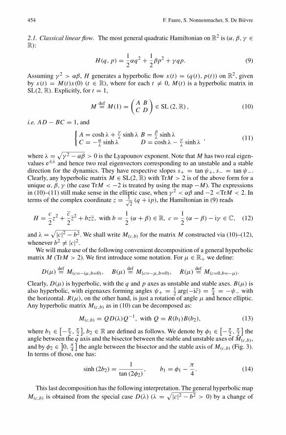
2.1. Classical linear flow. The most general quadratic Hamiltonian on R2 is (α, β, γ ∈
R):
H(q, p) = 1
2αq2 + 1
2βp2 + γ qp. (9)
Assuming γ 2 > αβ, H generates a hyperbolic flow x(t) = (q(t), p(t)) on R2, given
by x(t) = M(t)x(0) (t ∈ R), where for each t �= 0, M(t) is a hyperbolic matrix inSL(2,R). Explicitly, for t = 1,
Mdef= M(1) =
(A B
C D
)∈ SL (2,R) , (10)
i.e. AD − BC = 1, and{A = cosh λ+ γ
λsinh λ B = β
λsinh λ
C = −αλ
sinh λ D = cosh λ− γλ
sinh λ, (11)
where λ =√γ 2 − αβ > 0 is the Lyapounov exponent. Note thatM has two real eigen-
values e±λ and hence two real eigenvectors corresponding to an unstable and a stabledirection for the dynamics. They have respective slopes s+ = tanψ+, s− = tanψ−.Clearly, any hyperbolic matrix M ∈ SL(2,R) with TrM > 2 is of the above form for aunique α, β, γ (the case TrM < −2 is treated by using the map −M). The expressionsin (10)–(11) still make sense in the elliptic case, when γ 2 < αβ and −2 <TrM < 2. Interms of the complex coordinate z = 1√
2(q + ip), the Hamiltonian in (9) reads
H = c
2z2 + c
2z2 + bzz, with b = 1
2(α + β) ∈ R, c = 1
2(α − β)− iγ ∈ C, (12)
and λ =√|c|2 − b2.We shall write M(c,b) for the matrix M constructed via (10)–(12),
whenever b2 �= |c|2.We will make use of the following convenient decomposition of a general hyperbolic
matrix M (TrM > 2). We first introduce some notation. For µ ∈ R+ we define:
D(µ)def= M(c=−iµ,b=0), B(µ)
def= M(c=−µ,b=0), R(µ)def= M(c=0,b=−µ).
Clearly, D(µ) is hyperbolic, with the q and p axes as unstable and stable axes. B(µ) isalso hyperbolic, with eigenaxes forming angles ψ+ = 1
2 arg(−ic) = π4 = −ψ− with
the horizontal. R(µ), on the other hand, is just a rotation of angle µ and hence elliptic.Any hyperbolic matrix M(c,b) as in (10) can be decomposed as:
M(c,b) = QD(λ)Q−1, with Q = R(b1)B(b2), (13)
where b1 ∈[−π
2 ,π2
], b2 ∈ R are defined as follows. We denote by φ1 ∈
[−π2 ,
π2
]the
angle between the q axis and the bisector between the stable and unstable axes ofM(c,b),and by φ2 ∈
]0, π4
]the angle between the bisector and the stable axis ofM(c,b) (Fig. 3).
In terms of those, one has:
sinh (2b2) = 1
tan (2φ2), b1 = φ1 − π
4. (14)
This last decomposition has the following interpretation. The general hyperbolic mapM(c,b) is obtained from the special case D(λ) (λ =
√|c|2 − b2 > 0) by a change of
Scarred Eigenstates for Quantum Cat Maps of Minimal Periods 455
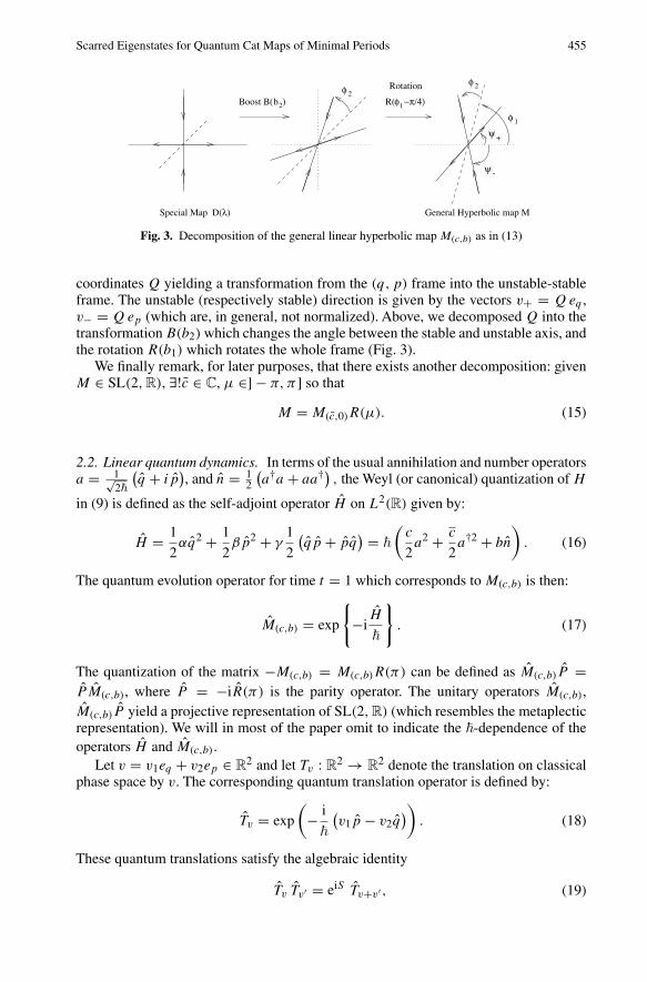
φ 2φ 2b2
φ 1
φ −π/4)R( Boost B( )
Rotation
General Hyperbolic map MSpecial Map D( )λ
1
+ψ
-ψ
Fig. 3. Decomposition of the general linear hyperbolic map M(c,b) as in (13)
coordinates Q yielding a transformation from the (q, p) frame into the unstable-stableframe. The unstable (respectively stable) direction is given by the vectors v+ = Qeq ,v− = Qep (which are, in general, not normalized). Above, we decomposed Q into thetransformationB(b2)which changes the angle between the stable and unstable axis, andthe rotation R(b1) which rotates the whole frame (Fig. 3).
We finally remark, for later purposes, that there exists another decomposition: givenM ∈ SL(2,R), ∃!c ∈ C, µ ∈]− π, π ] so that
M = M(c,0)R(µ). (15)
2.2. Linear quantum dynamics. In terms of the usual annihilation and number operatorsa = 1√
2�
(q + ip), and n = 1
2
(a†a + aa†
), the Weyl (or canonical) quantization of H
in (9) is defined as the self-adjoint operator H on L2(R) given by:
H = 1
2αq2 + 1
2βp2 + γ 1
2
(qp + pq) = �
(c
2a2 + c
2a†2 + bn
). (16)
The quantum evolution operator for time t = 1 which corresponds to M(c,b) is then:
M(c,b) = exp
{−iH
�
}. (17)
The quantization of the matrix −M(c,b) = M(c,b)R(π) can be defined as M(c,b)P =P M(c,b), where P = −iR(π) is the parity operator. The unitary operators M(c,b),M(c,b)P yield a projective representation of SL(2,R) (which resembles the metaplecticrepresentation). We will in most of the paper omit to indicate the �-dependence of theoperators H and M(c,b).
Let v = v1eq + v2ep ∈ R2 and let Tv : R
2 → R2 denote the translation on classical
phase space by v. The corresponding quantum translation operator is defined by:
Tv = exp
(− i
�
(v1p − v2q
)). (18)
These quantum translations satisfy the algebraic identity
Tv Tv′ = eiS Tv+v′ , (19)

456 F. Faure, S. Nonnenmacher, S. De Bievre
with S = 12�
(v2v
′1 − v1v
′2
) = − 12�v ∧ v′, so they generate an (irreducible) unitary
representation of the Heisenberg group. For any matrixM ∈ SL(2,R), one trivially hasM TvM
−1 = TMv . This intertwining persists at the quantum level:
M Tv M−1 = TMv. (20)
3. Classical and Quantum Automorphisms of the Torus
3.1. Classical automorphisms and their invariant manifolds. Consider the torus T =R
2/Z2 as a symplectic manifold with the two-form dq ∧ dp. Then any M ∈ SL(2,Z)defines a (discrete) symplectic dynamics on T in the obvious way. We are interested inthe case whereM is hyperbolic: the corresponding dynamical system is then an Anosovsystem [AA]. The stable and unstable manifolds of any point x ∈ T are obtained bywrapping the lines with slopes s± passing through x around the torus. We present heresome properties of these manifolds that we will need in subsequent sections.
A simple example we will use for numerical illustrations is the so called “Arnold’scat map” [AA]
MArnold =(
2 11 1
). (21)
Its Lyapounov coefficient is λ0 = log(
3+√52
)≈ 0.9624. The stable and unstable man-
ifolds of the fixed point x = 0 are depicted in Fig. 4.For any hyperbolic matrix M , the slopes s+ and s− of the unstable and stable direc-
tions are quadratic irrationals (i.e. the solutions of a quadratic equation with integercoefficients). It is well known [Kh] that any quadratic irrational s satisfies the followingdiophantine inequality:
∃C(s) > 0, ∀k ∈ Z, ∀l ∈ N∗,
∣∣∣∣s −k
l
∣∣∣∣ ≥ C(s)1
l2⇐⇒ |ls − k| ≥ C(s)1
l.
This means that quadratic irrationals are poorly approximated by rationals, in the sensethat, to get an approximation with an error ε, you need a rational with a denominator oforder at least ε−1/2.
0 0.5−0.5
0
0.5
−0.5
q
p
Fig. 4. The stable and unstable axes through 0 of the mapMArnold wrap around the torus at infinity. Wehave only represented the first six occurrences
Scarred Eigenstates for Quantum Cat Maps of Minimal Periods 457
This inequality will be used in the following manner. Consider the eigenvectors v±of M(c,b) defined as v+ = Qeq , v− = Qep (with Q the matrix defined in Eq. (13)). Asusual, their dual basis u± (defined as v+ · u+ = 1, v+ · u− = 0, etc.) can be used toexpress the coordinates of a point x in the basis v±:
x = q ′(x)v+ + p′(x)v−, with q ′(x) = x · u+, p′(x) = x · u−. (22)
We call d(x,Z2∗) the distance between a point x ∈ R2 and Z
2∗ = Z2 \ {0}, and we will
estimate it for x on the (un)stable axis:
∃C > 0, ∀x ∈ Rv±, d(x,Z2∗) ≥
C
‖x‖ + 1. (23)
To prove this, first note that, for any n ∈ Z s.t. nq �= 0, we have
|p′(n)| = |n · u−| = |u−,p|∣∣∣∣nq
u−,qu−,p
+ np∣∣∣∣ ≥
C(s+)|u−,p||nq | , (24)
where we have used the fact that u−,q/u−,p = s+ is a quadratic irrational. Interchangingnq and np, we obtain a first set of inequalities:
Lemma 1. There is a constant C (depending on M) such that, for any integer latticepoint n �= 0,
|p′(n)| ≥ C
‖n‖ and |q ′(n)| ≥ C
‖n‖ .
We can now prove (23) as follows. For each x ∈ Rv+, there exists an n ∈ Z2∗ so that
d(x,Z2∗) = ‖n− x‖ ≥ |n · u−|
‖u−‖ ≥ C±‖u−‖‖n‖ .
Since, obviously, ‖n− x‖ ≤ 1/√
2, (23) follows easily.We will in addition need a slightly refined statement. If the lattice point n �= 0 is in
a sufficiently thin strip around the unstable axis, it satisfies ‖p′(n)v−‖ ≤ 1/2 ≤ ‖n‖/2,which implies the lower bound |q ′(n)| ≥ ‖n‖
2‖v+‖ . Together with the above lemma, this
entails |p′(n)| ≥ C′1|q ′(n)| for a certain C′1. Interchanging p′ ↔ q ′, we see that the same
inequality holds for points in a sufficiently thin strip around the stable axis. Outside theunion of these strips, this inequality can be violated by at most a finite set of latticepoints; therefore, upon reducing the constant C′1 we obtain the main technical result ofthis section:
Lemma 2. There exists a constant Co > 0 (depending on M) such that, for any integerpoints n �= m of the plane, their coordinates along the (un)stable directions satisfy:
|q ′(n)− q ′(m)| ≥ Co
|p′(n)− p′(m)| . (25)
These inequalities precisely control the sparseness of the lattice points inside a striparound the unstable axis: the narrower the strip, the farther successive lattice points haveto be from each other.
458 F. Faure, S. Nonnenmacher, S. De Bievre
3.2. Quantum mechanics on the torus. We recall as briefly as possible the basic settingfor the quantum mechanics of a system with T as phase space, as well as the quantiza-tion of the automorphism M , referring to [HB, DE, BouDB] and references therein forfurther details. In order to define the Hilbert space associated to T, we first consider thetranslation operators T1 = T(1,0), T2 = T(0,1), which satisfy T1T2 = e−i/� T2T1 as aresult of (19). So for the values of � defined as:
N = 1
2π�∈ N
∗, (26)
one has the property[T1, T2
]= 0. The Hilbert space L2(R) may then be decomposed
as a direct integral of the joint eigenspaces of T1 and T2:
L2(R) =∫ ⊕
HN,θ
d2θ
(2π)2,
HN,θ ={|ψ〉 ∈ S ′(R) ∣∣ T1|ψ〉 = eiθ1 |ψ〉, T2|ψ〉 = eiθ2 |ψ〉
}. (27)
The “angle” θ = (θ1, θ2) ∈ [0, 2π [2 thus describes the periodicity properties of thewave function under translations by an elementary cell. HN,θ is N -dimensional.
We can define a projector Pθ from S(R) onto the space HN,θ :
Pθ =∑
(n1,n2)∈Z2
e−in1θ1−in2θ2 Tn11 T
n22 =
∑
n∈Z2
e−iθ ·n+iδn Tn. (28)
The phase δn = −n1n2Nπ comes from the decomposition Tn = e−iδn Tn11 T
n22 .
The Weyl quantization of a function f (x) = ∑k∈Z2 fk e2iπ(x∧k) is an operator on
HN,θ defined by
f =∑
k∈Z2
fk Tk/N . (29)
For |ψ〉 ∈ HN,θ , its “Wigner function” Wψ(x) is the distribution implicitly defined via
〈ψ |f |ψ〉 =∫
T
f (x) Wψ(x) dx, so that Wψ(k) = 〈ψ |Tk/N |ψ〉, (30)
where the Wψ(k) =∫T
e2iπ(x∧k) Wψ(x) dx are the Fourier coefficients of Wψ .Let now M ∈ SL(2,Z), so that A,B,C,D (see Eq. (10)) are integers. One then
easily deduces from (20) and (28) that the quantum map M satisfies:
M Pθ = Pθ ′ M, with θ ′ = θM−1 + 2πN
2(CD,AB) . (31)
The constant shift on the right-hand side (RHS) is due to the phases δn appearing in(28). M will define an endomorphism in HN,θ provided θ ′ ≡ θ mod 2π , i.e. providedθ is a fixed point of the dual map defined in (31). Given a hyperbolic matrix M , such afixed point exists for any N [DE]. In particular, for any matrix M the angle θ = (0, 0)(periodic wavefunctions) is a fixed point if N is even, while θ = (π, π) (antiperiodicwave wavefunctions) is a fixed point for N odd. We will always make this choice forour numerical examples.
Scarred Eigenstates for Quantum Cat Maps of Minimal Periods 459
From now on, we will assume that M = ±M(c,b) ∈ SL(2,Z) is a fixed hyperbolicmatrix defining a dynamics on the plane and on the torus. We will therefore no longerindicate its dependence on (c, b). We will also assume that � is such that (26) holds, andfor this � we select an angle such that θ ′ ≡ θ . In general, θ can depend on �, but we willnot indicate this dependence.
4. Coherent States and Their Evolution
4.1. Standard and squeezed coherent states. With the normalized state |0〉 defined bya|0〉 = 0, a “standard” coherent state is
|x〉 = Tx |0〉, x = (q, p) ∈ R2. (32)
More generally, we define for each c ∈ C∗ the “squeezed” coherent states |x, c〉 by
|c〉 = |0, c〉 = M(c,0)|0〉, |x, c〉 = Tx |c〉, (33)
where the “squeezing operator” M(c,0) is defined by (17), with b = 0. Note that, in viewof (15), given M ∈ SL(2,R), ∃!c ∈ C, σ ∈ [0, 2π [ such that
M|0〉 = eiσ |c〉. (34)
For more details on coherent states, we refer to [Z, Pe].To avoid confusion, we will use a tilde for the parameters of the squeezing opera-
tor M(c,0), and keep untilde notations for the parameters of the dynamics defined by
the matrix Mdef= ±M(c,b) that are at any rate kept fixed throughout the further discus-
sion. In the L2(R) representation, the state |x, c〉 is a Gaussian wave packet with meanposition q. Its Fourier transform is centered around the mean momentum p. For anystate |ψ〉 ∈ L2 (R), we define its Bargmann function as x �→ 〈x, c|ψ〉, and its Husimifunction to be the positive function Hc,ψ defined on phase space R
2 by:
Hc,ψ (x) =|〈x, c|ψ〉|2
2π�, which satisfies
∫
R2Hc,ψ (x) dx = ‖ψ‖2
L2(R). (35)
Note that for given |ψ〉, the Bargmann and Husimi functions depend on the choice ofc. Also, the function x �→ 〈x, c|ψ〉 is the product of a Gaussian factor with a functionholomorphic with respect to a c-dependent holomorphic structure. The term Bargmannfunction is usually reserved for the holomorphic factor, but we find it convenient to adopthere a slightly different convention.
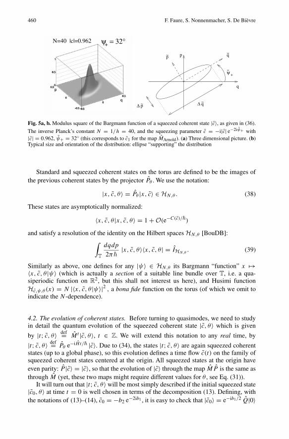
We will need the explicit expression of the (standard) Bargmann and Husimi functionsof the squeezed coherent state |c〉:
〈x, 0|c〉 = 1√cosh |c| exp
{−iqp tanh |c|
2�
}exp
{−1
2
(q2
�q2 +p2
�p2
)}. (36)
Here the unstable-stable frame (q, p) of the symmetric matrixM(c,0) is easily seen fromthe formulas in Sect. 2 to be obtained from (q, p) by a rotation of angle ψ+ (Fig. 4.1),and the widths are given by
�q2 = 2�
(1− tanh |c|) , �p2 = 2�
(1+ tanh |c|) . (37)
460 F. Faure, S. Nonnenmacher, S. De Bievre
+N=40 |c|=0.962 ψ = 32°
ψ~ +
∆
p
q
∆~q
~q
p~
p~
Fig. 5a, b. Modulus square of the Bargmann function of a squeezed coherent state |c〉, as given in (36).
The inverse Planck’s constant N = 1/h = 40, and the squeezing parameter c = −i|c| e−2iψ+ with|c| = 0.962, ψ+ = 32◦ (this corresponds to c1 for the map MArnold). (a) Three dimensional picture. (b)Typical size and orientation of the distribution: ellipse “supporting” the distribution
Standard and squeezed coherent states on the torus are defined to be the images ofthe previous coherent states by the projector Pθ . We use the notation:
|x, c, θ〉 = Pθ |x, c〉 ∈ HN,θ . (38)
These states are asymptotically normalized:
〈x, c, θ |x, c, θ〉 = 1+O(e−C(c)/�)and satisfy a resolution of the identity on the Hilbert spaces HN,θ [BouDB]:
∫
T
dqdp
2π�|x, c, θ〉〈x, c, θ | = IHN,θ
. (39)
Similarly as above, one defines for any |ψ〉 ∈ HN,θ its Bargmann “function” x �→〈x, c, θ |ψ〉 (which is actually a section of a suitable line bundle over T, i.e. a qua-siperiodic function on R
2, but this shall not interest us here), and Husimi functionHc,ψ,θ (x) = N |〈x, c, θ |ψ〉|2 , a bona fide function on the torus (of which we omit toindicate the N -dependence).
4.2. The evolution of coherent states. Before turning to quasimodes, we need to studyin detail the quantum evolution of the squeezed coherent state |c, θ〉 which is given
by |t; c, θ〉 def= Mt |c, θ〉, t ∈ Z. We will extend this notation to any real time, by
|t; c, θ〉 def= Pθ e−iH t/� |c〉. Due to (34), the states |t; c, θ〉 are again squeezed coherentstates (up to a global phase), so this evolution defines a time flow c(t) on the family ofsqueezed coherent states centered at the origin. All squeezed states at the origin haveeven parity: P |c〉 = |c〉, so that the evolution of |c〉 through the map MP is the same asthrough M (yet, these two maps might require different values for θ , see Eq. (31)).
It will turn out that |t; c, θ〉will be most simply described if the initial squeezed state|c0, θ〉 at time t = 0 is well chosen in terms of the decomposition (13). Defining, withthe notations of (13)–(14), c0 = −b2 e−2ib1 , it is easy to check that |c0〉 = e−ib1/2 Q|0〉

Scarred Eigenstates for Quantum Cat Maps of Minimal Periods 461
since M(c0,0) = R(b1)B(b2)R(−b1) and R(−b1)|0〉 = e−ib1/2 |0〉. Then, with M =QD(λ)Q−1,
Mt |c0〉 = e−ib1/2 Q D(λt)|0〉, 〈c0|Mt |c0〉 = 〈0|D(λt)|0〉 = 1√cosh(λt)
∈ R+,
(40)
so the overlap 〈c0|Mt |c0〉 is real positive for all times.For later purposes we note that, defining, for s ∈ R, cs ∈ C, σs ∈ [0, 2π [ by
e−i H�s |c0〉 = eiσs |cs〉, (41)
(see (34)), it is clear that 〈cs | e−iH t/� |cs〉 is real positive for all t . In fact, it can be shownthat the cs are the only values of c with this property. Among all s, s = 0 maximizes|〈0|cs〉|2, so |c0〉 is in a sense the most localized state among all |cs〉.
In this paper, we will almost exclusively build quasimodes from coherent states with“squeezing” c0; this choice is made for pure convenience, and our main semiclassicalresults apply to more general squeezings as well (see Sect. 6.6 and Appendix 10.2).
Before turning to |t; c, θ〉 ∈ HN,θ , we first describe the evolved state |t; c0〉 def=e−iH t/� |c0〉 ∈ L2(R), by studying its Husimi function on the plane, as defined in (35).It will be convenient (but again not absolutely necessary for our results, see Sect. 10.2)to adapt the choice of c in the definition of this Husimi function to the dynamics M byputting c = c0. One then computes
Hc0,t (x)def=
∣∣∣〈c0|T †x |t; c0〉
∣∣∣2
2π�=
∣∣∣〈0|Q†T†x QD (λt) Q
†Q|0〉∣∣∣2
2π�=
∣∣∣〈0|T †Q−1x
D (λt) |0〉∣∣∣2
2π�.
(42)
It is now natural to use the coordinates(q ′, p′
) = Q−1 (q, p) ∈ R2 attached to the
unstable-stable basis (v+, v−) (see Eq. (22)). In terms of these, the Husimi function is aGaussian drawn on the unstable and stable axes:
Hc0,t (x) =1
2π� cosh(λt)exp
(− q ′2
�q ′2− p′2
�p′2
), (43)
with
�q ′2 = 2�
1− tanh(λt)t→∞∼ � e2λt ,
�p′2 = 2�
1+ tanh(λt)= e−2λt �q ′2 t→∞→ �. (44)
The Husimi distribution of the evolved state |t; c0〉 therefore spreads exponentially (withrate λ) in the unstable direction of the map, and has a finite transverse width
√�. It “lives”
in an elliptic region of phase space centered on the origin and of area �q ′�p′ ∼ � eλt .Due to conservation of the total probability, the height of the distribution decreasesexponentially.
We now turn to |t; c0, θ〉 = Mt |c0, θ〉, t ≥ 0 and its Husimi function
Hc0,t,θ (x) = N |〈x, c0|Pθ |t; c0〉|2.
462 F. Faure, S. Nonnenmacher, S. De Bievre
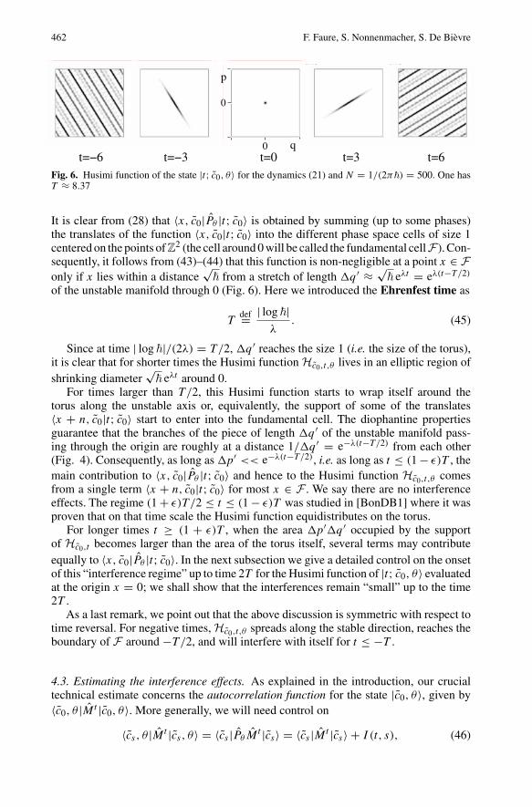
t=−6 t=−3 t=0
0
0 q
p
t=3 t=6Fig. 6. Husimi function of the state |t; c0, θ〉 for the dynamics (21) and N = 1/(2π�) = 500. One hasT ≈ 8.37
It is clear from (28) that 〈x, c0|Pθ |t; c0〉 is obtained by summing (up to some phases)the translates of the function 〈x, c0|t; c0〉 into the different phase space cells of size 1centered on the points of Z
2 (the cell around 0 will be called the fundamental cellF). Con-sequently, it follows from (43)–(44) that this function is non-negligible at a point x ∈ Fonly if x lies within a distance
√� from a stretch of length �q ′ ≈ √
� eλt = eλ(t−T/2)of the unstable manifold through 0 (Fig. 6). Here we introduced the Ehrenfest time as
Tdef= | log �|
λ. (45)
Since at time | log �|/(2λ) = T/2, �q ′ reaches the size 1 (i.e. the size of the torus),it is clear that for shorter times the Husimi function Hc0,t,θ lives in an elliptic region ofshrinking diameter
√� eλt around 0.
For times larger than T/2, this Husimi function starts to wrap itself around thetorus along the unstable axis or, equivalently, the support of some of the translates〈x + n, c0|t; c0〉 start to enter into the fundamental cell. The diophantine propertiesguarantee that the branches of the piece of length �q ′ of the unstable manifold pass-ing through the origin are roughly at a distance 1/�q ′ = e−λ(t−T/2) from each other(Fig. 4). Consequently, as long as�p′ << e−λ(t−T/2), i.e. as long as t ≤ (1− ε)T , themain contribution to 〈x, c0|Pθ |t; c0〉 and hence to the Husimi function Hc0,t,θ comesfrom a single term 〈x + n, c0|t; c0〉 for most x ∈ F . We say there are no interferenceeffects. The regime (1+ ε)T /2 ≤ t ≤ (1− ε)T was studied in [BonDB1] where it wasproven that on that time scale the Husimi function equidistributes on the torus.
For longer times t ≥ (1 + ε)T , when the area �p′�q ′ occupied by the supportof Hc0,t becomes larger than the area of the torus itself, several terms may contributeequally to 〈x, c0|Pθ |t; c0〉. In the next subsection we give a detailed control on the onsetof this “interference regime” up to time 2T for the Husimi function of |t; c0, θ〉 evaluatedat the origin x = 0; we shall show that the interferences remain “small” up to the time2T .
As a last remark, we point out that the above discussion is symmetric with respect totime reversal. For negative times, Hc0,t,θ spreads along the stable direction, reaches theboundary of F around −T/2, and will interfere with itself for t ≤ −T .
4.3. Estimating the interference effects. As explained in the introduction, our crucialtechnical estimate concerns the autocorrelation function for the state |c0, θ〉, given by〈c0, θ |Mt |c0, θ〉. More generally, we will need control on
〈cs , θ |Mt |cs , θ〉 = 〈cs |Pθ Mt |cs〉 = 〈cs |Mt |cs〉 + I (t, s), (46)
Scarred Eigenstates for Quantum Cat Maps of Minimal Periods 463
where we separated the contribution of the term n = (0, 0) (the “plane overlap”), fromthe remaining terms:
I (t, s)def=
∑
n∈Z2∗
e−in·θ+iδn 〈cs |Tn Mt |cs〉. (47)
This remainder represents the interference of the evolved plane coherent state with thelattice-translated initial state. We will show that these contributions tend to 0 asN →∞,uniformly for all times |t | ≤ 2(1− ε)T , for any fixed ε > 0.
A trivial upper bound is
|I (t, s)| ≤∑
n∈Z2∗
∣∣∣〈n, cs | e− i�H t |cs〉
∣∣∣ def= J0(t, s), (48)
and we shall estimate the RHS. Note that we extended I (t, s) in the natural way to realtimes t . The detailed proofs of the estimates below are given in Appendix 10.1; here welimit ourselves to explaining the underlying ideas and to an instructive comparison witha numerical example. For simplicity, we will concentrate on the case s = 0.
We define a time-dependent metric on the plane adapted to the Gaussian in (43):
‖ x ‖2t
def= 1
2
(q ′(x)�q ′(t)
)2
+ 1
2
(p′(x)�p′(t)
)2
.
The RHS of (48) is simply the sum of this Gaussian of heightHt = (cosh λt)−1/2 eval-uated at all nonzero integer lattice points. The diophantine properties proven in Sect. 3.1provide information on the position of the integer lattice with respect to the ellipse{‖x‖2
t = 1} and allow us to prove the following estimates:
• for relatively short times (meaning |t | ≤ (1 − ε)T ), all lattice points n �= 0 are faroutside the support of the Gaussian so that ‖n‖t is large. In fact, the distance ‖n‖treaches its minimum for a single point no (more precisely a finite number N of
points), with ‖no‖2t > c e−λ|t |
�>> 1. Note that, here and in the following, we write
f (�) << g(�) when lim�→0 f (�)/g(�) = 0. J0(t, 0) is dominated by the contri-bution of this finite set of points, given by N Ht exp
{−‖no‖2t
}, the contributions of
farther points being much smaller. The precise bound proven in the appendix reads:
|t | ≤ T �⇒ |I (t, 0)| ≤ 2√
2 e−λ|t |/2 exp
{−Co
e−λ|t |
2�
} [1+ C eλ(|t |−T )/2
],
(49)
where the constant Co is the parameter of the diophantine equation (25), and C canbe computed explicitly (it depends only on M).
• For times |t | ≥ T , a large number of lattice points (Nt = �q ′(t)�p′(t) ∼ eλ(|t |−T ))are contained in the ellipse (i.e. satisfy ‖n‖t ≤ 1), and their collective contributiondominates the RHS of (48): |I (t)| � NtHt ∼ eλ(−T+|t |/2). This is indeed essentiallywhat we prove:
T ≤ |t | �⇒ |I (t, 0)| ≤ 2π√
2
Coeλ(−T+|t |/2)
[1+ C′ eλ(T−|t |)/2
], (50)
where C′ can be computed explicitly in terms of M . This upper bound becomes oforder unity for |t | � 2T .
464 F. Faure, S. Nonnenmacher, S. De Bievre
• From the definition (46), we have trivially for any time
|I (t, 0)| ≤ 〈c0, θ |c0, θ〉 + 〈c0|Mt |c0〉 ≤ 1+O(
e−C(c0)/�)+ 1√
cosh(λ|t |) .
Combining these estimates (generalized to s �= 0), one obtains the following proposition:
Proposition 1. There exist positive constants C, C′, C′′ such that for all times t ∈ R,and for all s in a bounded interval
|I (t, s)| ≤ J0(t, s) ≤ min(C� eλ|t |/2, 1+
√2 e−λ|t |/2 +C′ e−C′′/�
). (51)
This shows that the interferences remain small until times of order 2T . The existenceof “short quantum periods” for certain values of � (see the introduction and Sect. 8)implies that I (t, 0) is of order 1 at t = P � 2T for these values of �. This is furtherillustrated in Fig. 7.
Figure 7 shows numerical calculations of log |I (t, 0)| for values of Planck’s “con-stant” N = 9349 → 9359 and compares them to F(t), which is essentially given bythe upper bounds (49)–(50). We observe that, whereas (49) is close to optimal, the sameis not true for (50) for most values of N : there is a “plateau” log |I (t, 0)| � log(�1/2)
for t > T ′, where T ′ = log(N)/λ is a shifted Ehrenfest time. This plateau can beexplained by assuming that the phases which multiply the different terms in I (t, 0) areuncorrelated, like independent random phases. For t >> T , the RHS of (47) couldthen be replaced by a sum of many (� Nt ) terms with identical moduli Ht but randomuncorrelated phases, similar to a 2-dimensional random walk. The modulus of the sum(i.e. the length of the random walk) has a typical value |I (t, 0)| ∼ √Nt Ht ∼ �
1/2,independent of time: this is indeed what we see numerically.
However, for the value of N = 9349, corresponding to a “short quantum period”P = 19, as discussed in Sect. 8, log |I (t, 0)| is close to the upper bounds (49)–(50)
0 2 4 6 8 10 12 14 16 18 20-10
-8
-6
-4
-2
0
L
log(h )1/2
F(t)
t
log |I(t,0)|for 1/h=N=9350 9359
2T’T’
log |I(t,0)| for 1/h=N=9349
Fig. 7. Numerical calculations of log |I (t, 0)|, for the map (21). The heuristic upper bound F(t) (solidline) is defined in terms of the shifted Ehrenfest time T ′ = log(N)/λ: F(t) = − λt
2 − eλ(T′−t)−1 for
0 < t < T ′ and F(t) = λ2
(t − 2T ′
) + 0.5 for T ′ < t < 2T ′. The horizontal dashed line at log(h1/2)
gives the order of magnitude of the plateau for t > T ′
Scarred Eigenstates for Quantum Cat Maps of Minimal Periods 465
up to time P � 2T ′. In such exceptional cases – crucial in this paper – there appearsstrong correlations between the phases in the sum I (t, 0): the random walk somehowbecomes “rigid”, which makes its total length of the same order as the sum of individuallengths, |I (t, 0)| ∼ J0(t, 0) ∼ NtHt . This rigidity can actually by analyzed directlyfrom the explicit expression for the phases [FN2]: one first finds that for these specialvalues of Planck’s constant N = Nk and t in the interval T < t < 2T , the phases cor-responding to the relevant ∼ Nt lattice points are all close to 2d th roots of unity, whered = (trM)2 − 4 (in the example M = MArnold and Nk = 9349, the relevant phases areall close to unity). Then, the sum of these ∼ Nt phases behaves like G(M,Nk)Nt forNt >> 1, and one can check that the prefactor G(M,Nk) (a Gauss sum) is boundedaway from zero uniformly (e.g. G(MArnold, 9349) = 1). This explains the behaviour|I (t, 0)| ∼ J0(t, 0). This situation drastically differs from the case of a “generic” N ,where the relevant phases are more or less equidistributed over the circle.
5. Quasimodes at the Origin
5.1. Continuous time versus discrete time quasimodes. We are now ready to study thequasimodes (2) and (6) “associated” with the periodic orbits of the dynamics generatedbyM , as discussed in the introduction. To alleviate the notations, we start with the casewhere the orbit is simply the fixed point (0, 0) ∈ T. The rather straightforward general-ization to arbitrary orbits is given in Sect. 7. Note that the Ehrenfest time T = | ln �|
λis
in general not an integer: whenever T or T/2 appears in a sum boundary, they shouldtherefore be replaced by the nearest integer.
It will be convenient to also consider slightly modified quasimodes, for which theinitial state is not the squeezed coherent state |c0, θ〉 as in (2), but rather the followingsuperposition of squeezed coherent states:
Pθ
∫ 1
0dt e−iφt e−
i�H t |c0〉. (52)
The “continuous time” version of the quasimodes defined in (2) then reads:
|�contφ 〉 def= P−T ,T ,φ Pθ
∫ 1
0dt e−iφt e−
i�H t |c0〉 (53)
= Pθ
∫ T
−Tdt e−iφt e−
i�H t |c0〉. (54)
Here we introduced, for any φ ∈ R, t0 < t1 ∈ Z, the operator
Pt0,t1,φ =t1−1∑
t=t0e−itφ Mt , (55)
and the equality (54) follows from a trivial computation.These quasimodes can also be decomposed into 4 parts |�cont
j,φ 〉, obtained by integrat-ing in t over time intervals of length T/2, then projecting the obtained state in HN,θ . Aremarkable and useful property (derived from Poisson’s formula) is that we can recoverthe “discrete time” quasimodes |�disc
φ 〉 defined in (2) from the “continuous time” ones:
|�discφ 〉 =
∑
k∈Z
|�contφ+2πk〉.
466 F. Faure, S. Nonnenmacher, S. De Bievre
Notice that the state in (52) is not 2π -periodic with respect to φ so that the quasimodes|�cont
φ 〉 depend on the “quasienergy” φ ∈ R.The main reason for considering continuous time quasimodes is that they are easily
connected with generalized eigenstates of the Hamiltonian H , which allows to pointwisedescribe their Husimi densities, a task we turn to in Sect. 6.
In the next subsection, we start our study of the above quasimodes. We will use fromnow on the notation |�φ〉 in statements that are valid both for |�disc
φ 〉 and |�contφ 〉 (and
similarly for |�j,φ〉).
5.2 Orthogonality of the states |�j,φ〉n at fixed φ
Proposition 2. (i) The states |�j,φ〉, j = 1, 2, 3, 4 and |�φ〉 satisfy, as � → 0
〈�j,φ |�j,φ〉 = T
2S1(λ, φ)+O(1), 〈�φ |�φ〉 = 2T S1(λ, φ)+O(1), (56)
where the smooth function S1(λ, φ) is strictly positive for all φ ∈ R and O(1) isuniformly bounded in φ. In particular these states do not vanish for small enough� and the normalized quasimodes |�φ〉n satisfy (5).
(ii) Furthermore, for all φ ∈ R, the |�j,φ〉n become mutually orthogonal in the semi-classical limit: for all j �= k ∈ {1, . . . , 4}
lim�→0
n〈�j,φ |�k,φ〉n = 0. (57)
The limit is uniform for all φ in a bounded interval.(iii) Consequently, for all φ ∈ R,
n〈�φ |�j,φ〉n → 1/2, n〈�φ |�erg,φ〉n → 1/√
2 and n〈�φ |�loc,φ〉n → 1/√
2.
Proof. (i) We first give a detailed proof for the “continuous time” quasimodes. Writingk = j − i ∈ {0, 1, 2, 3}, a simple computation yields (see (41))
〈�conti,φ |�cont
j,φ 〉
=T2 −1∑
t=0
T2 −1∑
t ′=0
∫ 1
0ds
∫ 1
0ds′ e−i(t−t ′+s−s′+kT /2)φ 〈c0|Pθ e−
i�H (t−t ′+s−s′+kT /2) |c0〉.
Using (46) and (48) this becomes:
〈�conti,φ |�cont
j,φ 〉=∫ T/2
−T/2ds
(T
2− |s|
)e−i(s+kT /2)φ〈c0| e− i
�H (s+kT /2) |c0〉 + error, (58)
where
error ≤∫ 1
0ds
∫ 1
0ds′
T2 −1∑
t=− T2
(T2− |s|) J0(t + k T
2+ s − s′, s′).
Using the bound (51), one readily finds that the second term is O(� 3−k4 ).
Scarred Eigenstates for Quantum Cat Maps of Minimal Periods 467
To estimate the norm of |�contj 〉, there remains to compute the integral in (58) in the
case i = j , that is k = 0:∫ T/2
−T/2ds (T /2− |s|) e−isφ〈c0| e− i
�H s |c0〉 =
∫ T/2
−T/2ds(T /2− |s|) e−isφ
√cosh(λs)
= T
2Scont
1 (λ, φ, T /2)− Scont2 (λ, φ, T /2),
where the (real) functions Scont1 , Scont
2 are defined as follows:
Scont1 (λ, φ, τ )
def=∫ τ
−τdt
e−itφ
√cosh (λt)
, Scont2 (λ, φ, τ )
def=∫ τ
−τdt
|t | e−itφ
√cosh (λt)
. (59)
The limits of Sconti (λ, φ, τ ) as τ → ∞ clearly exist. We only give the value for Scont
1 ,the most relevant one for our purposes [BaTIT]:
Scont1 (λ, φ)
def= limτ→∞ S
cont1 (λ, φ, τ ) = 1
λ√
2π
∣∣∣∣�(
1
4+ i
φ
2λ
)∣∣∣∣2
. (60)
For fixed λ, this function is maximal for φ = 0 (with value≈ 5.244/λ), and decreases as√4πλ|φ| e−π |φ|/2λ for |φ| → ∞. A crucial property is the strict positivity of this function,
for all values λ > 0, φ ∈ R.The computation of 〈�φ |�φ〉 is similar.
(ii) We now estimate the overlaps 〈�i,φ |�j,φ〉 for j �= i, by estimating the first integralof (58) in the cases 3 ≥ k ≥ 1:∣∣∣∣∣
∫ T/2
−T/2ds (T /2− |s|) e−i(s+kT /2)φ
√cosh(λ(s + kT /2))
∣∣∣∣∣ ≤4√
2
λ2e−
λ(k−1)T4 = O(� k−1
4 ).
Taking into account the estimate of the error in (58), we see that for any i �= j , theoverlap 〈�cont
i,φ |�contj,φ 〉 is bounded by a constant (even by O(�1/4) for |i − j | = 2). As a
result,
∀i �= j, n〈�conti,φ |�cont
j,φ 〉n =〈�cont
i,φ |�contj,φ 〉
〈�conti,φ |�cont
i,φ 〉≤ C
T. (61)
This proves (ii). Part (iii) is now obvious.To treat the case of the discrete quasimodes, the integrals over time have to be replaced
by sums over integers. For instance, the expressions defined in (59) are replaced by
Sdisc1 (λ, φ, τ )
def=∑
|t |≤τ
e−itφ
√cosh (λt)
,
and similarly for S2. The sum Sdisc1 (λ, φ) = limτ→∞ Sdisc
1 (λ, φ, τ ) is also nonnegativefor all λ > 0, φ ∈ [−π, π ]. Indeed, Poisson’s formula induces the identity
Sdisc1 (λ, φ) =
∑
k∈Z
Scont1 (λ, φ + 2kπ).
The norms of the discrete quasimodes therefore satisfy an estimate similar to (57),upon replacing Scont
1 by Sdisc1 . The other estimates are identical as for the continuous
version. ��
468 F. Faure, S. Nonnenmacher, S. De Bievre
5.3. Quasimodes of different quasienergies. We now compare quasimodes |�φ〉 of dif-ferent quasienergies and show:
Proposition 3. Let φ0 be an arbitrary angle in [0, 2π [, and
φk = φ0 + π
Tk, k = 1, . . . , 2T .
The 2T quasimodes |�φk 〉n become mutually orthogonal in the semiclassical limit:∀k′ �= k, n〈�φk′ |�φk 〉n = O(1/T ).
This is an immediate consequence of the following finer estimate:
Proposition 4. Let I ⊂ R be a fixed bounded interval. There exists a constant C > 0such that, given any semiclassically vanishing function θ(�) and n ∈ Z
∗, if φ, φ′ ∈ I ,and if the phase shift �φ = φ′ − φ satisfies |�φ − nπ
T| ≤ θ(�)
|n|T
, then we have, forsmall enough �, n〈�φ′ |�φ〉n ≤ C
(θ(�)+ 1
T
).
Proof. As before, we write the proof for the continuous time quasimodes. The over-lap 〈�cont
φ′ |�contφ 〉 is given by an expression similar to (58). Using the estimate (51) for
I (t, s), we obtain
〈�contφ′ |�cont
φ 〉 =∫ T
−Tdt
∫ T
−Tdt ′
ei(t ′φ′−tφ)√
cosh λ(t − t ′) +O(1)
=∫ 2T
−2Tds
eisφ
√cosh(λs)
sin {�φ (T − |s|/2)}�φ/2
+O(1),
where we introduced φdef= φ′+φ
2 . This integral is bounded above by 2S1(λ,0)|�φ| , so that
for a phase difference bounded away from zero (i.e. |�φ| ≥ c > 0), the scalar productof the normalized states is n〈�φ′ |�φ〉n = O(T −1). We are however more interestedin the case where �φ is �-dependent and semiclassically small: �φ → 0. Inserting| sin{�φ(T −|s|/2)}− sin{�φT }| ≤ |s|�φ/2 in the integral and using (56), we get for� → 0, �φ→ 0:
n〈�contφ′ |�cont
φ 〉n = Scont(φ)√Scont(φ)Scont(φ′)
sin (T �φ)
T�φ+O(1/T ).
The first term can be as large as 1, for �φ << T −1. It will also be large for values�φ = π(n+1/2)
Twith n an integer, |n| << T , where it takes the value ±1/T�φ. At the
opposite extreme, the term vanishes for�φ = nπT
, n a nonzero integer, and close to thisvalue it behaves like (−1)n T
πn(�φ − nπ
T). ��
We are now set to analyze, in the next subsections, the phase space distributions ofthe quasimodes |�φ〉n and of their components.
Scarred Eigenstates for Quantum Cat Maps of Minimal Periods 469
5.4. Localization of |�loc,φ〉n near the origin. Recall that |�loc,φ〉 = |�2,φ〉 + |�3,φ〉.We will show the following:
Proposition 5. Let φ ∈ R. Then, for any f ∈ C∞(T2),
lim�→0
n〈�loc,φ |f |�loc,φ〉n = f (0) and lim�→0
∫
T
f (x)Hc0,loc,φ,θ (x) dx = f (0),
(62)
where Hc0,loc,φ,θ (x) = N |〈x, c0, θ |�loc,φ〉n|2 is the Husimi function of |�loc,φ〉n. Itfollows that the semiclassical measures Hc0,loc,φ,θ (x)dx and the Wigner distributionconverge to the delta measure at the origin. All limits are uniform for φ in a boundedinterval.
Using a more physical terminology, one can say that the quasimodes |�loc,φ〉nstrongly scar (or localize) on the fixed point 0 ∈ T
2 of the map M .
Proof. As before, we write the proof for |�contloc,φ〉, given by
|�contloc,φ〉 = Pθ
∫ T/2
−T/2dt e−iφt |t; c0〉.
This is a sum of evolved coherent states for times |t | ≤ T/2. At this maximal time, the
length�q ′ of the Husimi function of e−i�H t |c0〉 reaches the size of the torus. To control
the contribution of the nonlocalized states at t ≈ T/2, we first select a function �(�)such that in the small-� limit 1 << �(�) << T . We then split |�cont
loc,φ〉 in two pieces:
|�contloc,φ〉 = Pθ
∫
|t |≤τ∗dt e−iφt |t; c0〉 + Pθ
∫
τ∗≤|t |≤ T2
dt e−iφt |t; c0〉
= |�′〉 + |�′′〉,where τ∗
def= [T/2−�(�)/λ]. From the proof of Proposition 2 it is clear that
〈�′|�′〉 ∼ 2τ∗Scont1 (λ, φ) ∼ T Scont
1 (λ, φ) ∼ 〈�loc,φ |�loc,φ〉 when � → 0. (63)
The norm of the remainder |�′′〉 is estimated similarly:
〈�′′|�′′〉 ∼ �
λScont
1 (λ, φ) ≤ C�(�) = o(T ). (64)
In the interval |t | ≤ τ∗, the ellipses supporting the states |t; c0〉 have lengths√
� eλt ≤e−�(�) → 0. Considering the diskD� centered at the origin and of radius e−�(�)/2, theHusimi functions of these states are therefore semiclassically concentrated inside D�.We will show below that |�cont
loc,φ〉n is also concentrated inside this disk.
Using (63) and (64), together with the obvious |a + b|2 ≤ 2(|a|2 + |b|2), one finds∫
T\D�N |〈x, c0, θ |�cont
loc,φ〉n|2 dx ≤C
T
∫
T\D�N(|〈x, c0, θ |�′〉|2 + |〈x, c0, θ |�′′〉|2
)dx
≤ C
T
(∫
T\D�N |〈x, c0, θ |�′〉|2 dx + 〈�′′|�′′〉
)(65)
≤ C�(�)
T. (66)
470 F. Faure, S. Nonnenmacher, S. De Bievre
The last inequality comes from the observation that the Bargmann function 〈x, c0, θ |�′〉is a sum of Gaussians of widths smaller than e−�(�) so simple analysis shows that theintegral in (65) is O (
N exp(−c e�(�))). Consequently, (66) holds and yields the prop-
osition provided we choose log logN << � << logN . For discrete quasimodes, weonly need to replace Scont
1 by Sdisc1 in the above estimate. ��
For later purpose, we notice that the previous proof can be applied to the states
|�contt1,t2
〉 = Pθ
∫ t2
t1
eiφt |t; c0〉, with − T
2≤ t1 ≤ 0 ≤ t2 ≤ T
2. (67)
These states indeed localize at the origin in the sense of Eqs. (62) and (66). The sameis obviously true for the discrete analogues of these states: |�disc
t1,t2〉 = Pt1,t2 |c0, θ〉. Note
that |�2,φ〉 and |�3,φ〉 are of this type.
5.5. Equidistribution of |�erg,φ〉n. Recalling that |�erg,φ〉 = |�1,φ〉 + |�4,φ〉 we have
Proposition 6. Let φ ∈ R. Then, for any f ∈ C∞(T2)
lim�→0
n〈�erg,φ |f |�erg,φ〉n =∫
T
f (x)dx = lim�→0
∫
T
f (x)Hc0,erg,φ,θ (x) dx, (68)
where Hc0,erg,φ,θ (x) = N |〈x, c0, θ |�loc,φ〉n|2 is the Husimi function of |�erg,φ〉n. Itfollows that the Husimi measure Herg,φ(x) dx and the Wigner distribution converge tothe Liouville measure on the torus. The limits are uniform for φ in a bounded interval.
The states |�erg,φ〉 are said to semiclassically equidistribute on the torus.
Proof. We will use the algebraic structure of the quantized automorphisms in the proof.We will drop the index φ from the notations. It is clearly enough to show that, for eachk ∈ Z
2∗, we have
lim�→0
〈�erg|Tk/N |�erg〉 = 0.
For that purpose, we write
〈�erg|Tk/N |�erg〉= 〈�1|Tk/N |�1〉 + 〈�4|Tk/N |�4〉 + 〈�1|Tk/N |�4〉 + 〈�4|Tk/N |�1〉. (69)
We first estimate the two diagonal terms of the RHS. Using |�1〉 = eiφT M−T |�3〉,|�4〉 = e−iφT MT |�2〉 and the intertwining property (20), we get
〈�1|Tk/N |�1〉 + 〈�4|Tk/N |�4〉 = 〈�3|Tk+|�3〉 + 〈�2|Tk−|�2〉.
Here k±def= M±T k/N ∈ (Z/N)2 are of order 1 (see below), so that we transformed the
“microscopic” translation by k/N (of order �) into “macroscopic” ones. Each term istherefore the overlap between the state |�2〉 or |�3〉 localized in a small disc D� cen-tered at the origin of the torus (cf. Eqs. (65,67)), and a translated state localized in the
discD�,±def= D�+k± centered at the point k± mod Z
2. This overlap will consequently

Scarred Eigenstates for Quantum Cat Maps of Minimal Periods 471
be small provided k± is sufficiently far away from the integer lattice. We prove this factusing (22):
k+ = q ′(k) eT λ /N v+ + p′(k) e−T λ /N v− = C(N)q ′(k)v+ +O(�2)v−,k− = q ′(k) e−T λ /N v+ + p′(k) eT λ /N v− = C(N)p′(k)v− +O(�2)v+,
where 2π e−λ ≤ C(N) ≤ 2π eλ since T/2 is the closest integer to | ln �|/2λ. Now,q ′(k) �= 0 �= p′(k) since the slopes of v± are irrational. Consequently, k± are at a finitedistance from Z
2 for small enough �, and the disks D� and D�,± do not intersect eachother. We can thus estimate the overlap:
n〈�3|Tk+|�3〉n =∫
T
n〈�3|x, c0, θ〉 〈x, c0, θ |Tk+|�3〉N dxn
={∫
T\D�+∫
D�
}n〈�3|x, c0, θ〉 〈x, c0, θ |Tk+|�3〉n N dx.
Using the Cauchy-Schwarz inequality, the first integral is bounded as
∣∣∣∫
T\D�n〈�3|x, c0, θ〉 〈x, c0, θ |Tk+|�3〉n N dx
∣∣∣
≤√∫
T\D�Hc0,3,θ (x) dx
√∫
T\D�Hc0,3,θ (x − k+) dx ≤ C
√�
T,
where we used (65) applied to |�3〉. The integral overD� is treated similarly, exchangingthe roles of both factors: now the second factor semiclassically converges to zero due tothe inclusion D� ⊂ (T \D�,+). In the end, we get for log logN << �(�) << logN ,
n〈�1|Tk/N |�1〉n = n〈�3|MT Tk/NM−T |�3〉n = O
(√�(�)
T
), (70)
uniformly for φ in a finite interval. The proof goes through unaltered for the secondoverlap n〈�4|Tk/N |�4〉n and in fact for any MT |�t1,t2〉n as in (67), leading to:
Lemma 3. Consider a semiclassically diverging function log | log �| << �(�) <<
| log �| and k ∈ Z2∗. Given a bounded interval, there exists a constant C so that for all
φ in the interval
∣∣n〈�t1,t2 |M−T Tk/NMT |�t1,t2〉n
∣∣ ≤ C√�(�)
T.
As a result, the states MT |�t1,t2〉n equidistribute as � → 0, which implies that theintegral of their Husimi function over a fixed domain of area A converges to A. We nowuse this information to finish the proof of Proposition 6.
We enlarge Fig. 1 and define the additional state |�5〉 = e−iφT MT |�3〉, which,according to Lemma 3, equidistributes. Now, using the same intertwining property asabove, we rewrite the nondiagonal terms in the RHS of (69) as
〈�2|MT/2Tk/NM−T/2|�5〉+〈�5|MT/2Tk/NM
−T/2|�2〉 = 〈�2|Tk′ |�5〉+〈�5|Tk′ |�2〉,
472 F. Faure, S. Nonnenmacher, S. De Bievre
with the vector k′ def= MT/2k/N . Each term is the overlap between a state localized nearthe origin (e.g. 〈�2|) and an equidistributed one (e.g. Tk′ |�5〉). It is natural to expectthat they are asymptotically orthogonal.
To prove this fact, we proceed as above:
∣∣n〈�2|Tk′ |�5〉n
∣∣ ≤√∫
T\D(r)dxHc0,2,θ (x)
√∫
T\D(r)dxHc0,5,θ (x − k′)
+√∫
D(r)
dxHc0,2,θ (x),
√∫
D(r)
dxHc0,5,θ (x − k′), (71)
where D(r) is the disc of radius r centered at 0. Using the semiclassical localization of|�2〉n at the origin and the equidistribution of |�5〉n, we find
lim sup�→0
|n〈�2|Tk′ |�5〉n| ≤√πr.
Since this is true for any r > 0, lim�→0 |n〈�2|Tk′ |�5〉n| = 0. We now control all theterms of (69) and after taking care of the normalizations we obtain Proposition 6. ��
5.6. Semiclassical properties of |�φ〉 = |�loc,φ〉 + |�erg,φ〉. We now finally considerthe “full” quasimode |�φ〉. It is the sum of two states, one localized, the second equi-distributed.
Proposition 7. For any φ ∈ R, (7) holds with τ = 1, x0 = 0. The limit is uniform for φbelonging to a bounded interval.
Proof. It is again enough to study n〈�|Tk/N |�〉n and to show
lim�→0
n〈�|Tk/N |�〉n = 1
2(1+ δk,0).
The results of the previous subsections imply immediately that this reduces to showing
lim�→0
n〈�loc|Tk/N |�erg〉n = 0.
This in turn is proven as in the previous subsection through the use of the Cauchy-Sch-warz inequality and cutting the integral over T into the integral over a small disc aroundthe origin and an integral over the complement (see (71)). ��
To conclude this section, let us remark that the semiclassical properties of the variousquasimodes we introduced are not altered if we replace T in the sum or integrationboundaries by an integer that differs from it by a finite amount, bounded as � goes tozero. This will occasionally be useful in the sequel.
Scarred Eigenstates for Quantum Cat Maps of Minimal Periods 473
6. Pointwise Description of the Quasimodes
In the last sections, we showed that the Husimi and Wigner functions of the quasimodes|�φ〉n converge to the measure 1+δ0
2 in the semiclassical limit. The crucial tools of the
proof were, on the one hand, precise estimates of the overlaps 〈c0, θ |Mt |c0, θ〉 (obtainedusing the diophantine properties of the invariant axes), on the other hand the algebraicintertwining between M and the quantum translations.
Still, it would be interesting to know the speed at which this convergence takes place,or to compute more refined “indicators” of the localization of the quasimodes.
In this section, we will use a more “direct” yet slightly more cumbersome route whichwill yield more precise information on the phase space distribution of the “continuoustime” quasimodes. The main step of this route is the pointwise description of the Barg-mann and Husimi functions of |�cont
φ 〉. This description will then provide an estimateof the speed of convergence to the limit semiclassical measure; at the same time, it willallow us to compute alternative localization indicators, like the Ls-norms of the Husimifunctions. The pointwise estimates will also uncover the “hyperbolic” structure of theHusimi functions near the origin, a structure already emphasized by several authorsfor finite-time quasimodes [KH, WBVB] and for spectral Wigner and Husimi functions[ROdA].
6.1. Plane quasimodes. Our final objective is to estimate the Bargmann function〈x, c0, θ |�cont
φ 〉 for x ∈ F the fundamental domain. For this purpose, we start from
quasimodes of the Hamiltonian H :
|�φ,t 〉 def=∫ t
−tds e−iφs e−iH s/� |c0〉. (72)
The torus quasimode |�contφ 〉 is obtained by projecting |�φ,T 〉 onto HN,θ (cf. Eq. (54)).
In this subsection, we will study the Bargmann function of the plane quasimode |�φ,T 〉.Using the rescaled variable Z
def= q ′−ip′2√
�, this function is given by the following
integral:
�φ,T (x)def= 〈x, c0|�φ,T 〉 = e−|Z|2
∫ T
−Tds
e−iφs
√cosh λs
eZ2 tanh λs . (73)
Through the change of variables U = Z2(1 − tanh λs), and using the parameter
µdef= 1/4+ iφ/2λ, this integral may be rewritten as
�φ,T (x) =eZ
2−|Z|2
λ2µ+1/2Z2µ
∫ U1
U0
dU
UUµ e−U
(1− U
2Z2
)−µ−1/2
, (74)
with the boundaries U0 = Z2(1 − tanh λT ) � 2Z2�
2, U1 = Z2(1 + tanh λT ) �2Z2(1−�
2). This function satisfies the following symmetries (with obvious notations):
�φ,T (Z) = �φ,T (−Z) = �−φ,T (iZ). (75)
The hyperbolic Hamiltonian H admits no bound state in L2(R), but for any realenergyE = −�φ, it has two independent generalized eigenstates, distinguished by their
474 F. Faure, S. Nonnenmacher, S. De Bievre
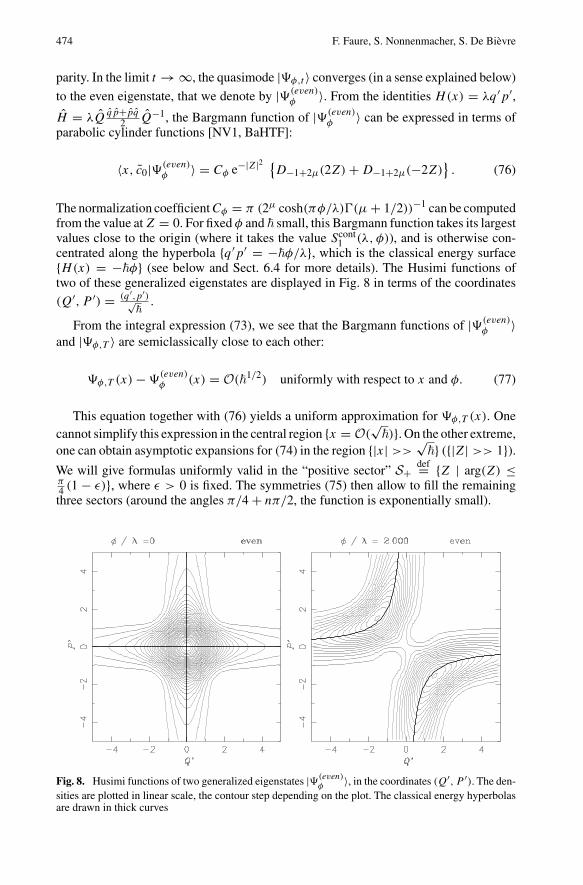
parity. In the limit t →∞, the quasimode |�φ,t 〉 converges (in a sense explained below)
to the even eigenstate, that we denote by |�(even)φ 〉. From the identities H(x) = λq ′p′,H = λQ
qp+pq2 Q−1, the Bargmann function of |�(even)φ 〉 can be expressed in terms of
parabolic cylinder functions [NV1, BaHTF]:
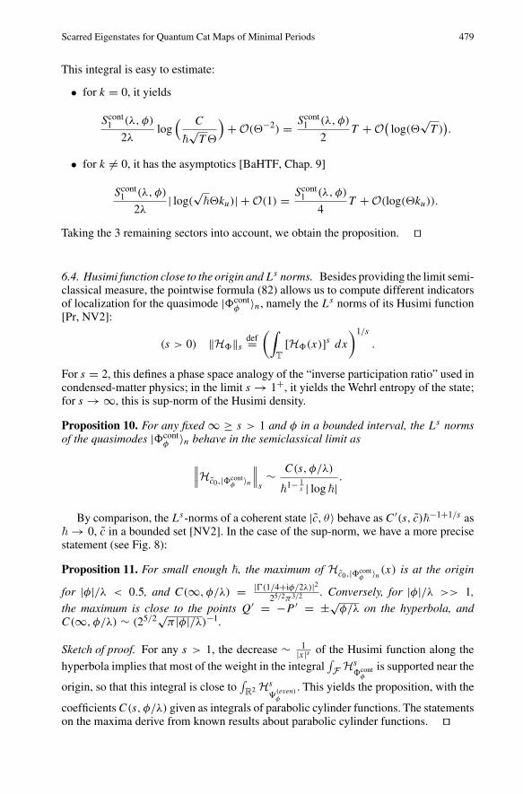
〈x, c0|�(even)φ 〉 = Cφ e−|Z|2{D−1+2µ(2Z)+D−1+2µ(−2Z)
}. (76)
The normalization coefficientCφ = π (2µ cosh(πφ/λ)�(µ+ 1/2))−1 can be computedfrom the value atZ = 0. For fixed φ and � small, this Bargmann function takes its largestvalues close to the origin (where it takes the value Scont
1 (λ, φ)), and is otherwise con-centrated along the hyperbola {q ′p′ = −�φ/λ}, which is the classical energy surface{H(x) = −�φ} (see below and Sect. 6.4 for more details). The Husimi functions oftwo of these generalized eigenstates are displayed in Fig. 8 in terms of the coordinates(Q′, P ′) = (q ′,p′)√
�.
From the integral expression (73), we see that the Bargmann functions of |�(even)φ 〉and |�φ,T 〉 are semiclassically close to each other:
�φ,T (x)−�(even)φ (x) = O(�1/2) uniformly with respect to x and φ. (77)
This equation together with (76) yields a uniform approximation for �φ,T (x). Onecannot simplify this expression in the central region {x = O(√�)}. On the other extreme,one can obtain asymptotic expansions for (74) in the region {|x| >> √
�} ({|Z| >> 1}).We will give formulas uniformly valid in the “positive sector” S+ def= {Z | arg(Z) ≤π4 (1 − ε)}, where ε > 0 is fixed. The symmetries (75) then allow to fill the remainingthree sectors (around the angles π/4+ nπ/2, the function is exponentially small).
Fig. 8. Husimi functions of two generalized eigenstates |�(even)φ 〉, in the coordinates (Q′, P ′). The den-sities are plotted in linear scale, the contour step depending on the plot. The classical energy hyperbolasare drawn in thick curves
Scarred Eigenstates for Quantum Cat Maps of Minimal Periods 475
Expanding the last factor in the integral (74) into powers of 1/Z2, we get a sum ofincomplete Gamma functions [BaHTF, Chap. 9]:
∫ U1
U0
dU
UUµ e−U
(1− U
2Z2
)−µ−1/2
= (γ (µ,U0)− γ (µ,U1)
)+ µ+ 1/2
2Z2
(γ (µ+ 1, U0)− γ (µ+ 1, U1)
)+ . . . .These gamma functions have simple asymptotics in two regimes:
• for U0 << 1 << U1, that is, x ∈ S+,√
� << |x| << 1√�
, they yield
�φ,T (x) = �(µ) eZ2−|Z|2
λ2µ+1/2Z2µ
(1+O
(1
|Z|2)+O(
√�Z)
)
= �(µ)
λ21/2−µ�µ
(q ′ − ip′)2µe−
p′2+iq′p′2�
(1+O
(�
|x|2)+O(
√�1/2|x|)
).
(78)
This asymptotics also holds for the Bargmann function of |�(even)φ 〉 in the sector|Z| >> 1, Z ∈ S+: it indeed corresponds to known asymptotics of the paraboliccylinder functions D−1+2µ [BaHTF, Chap. 8]. This gives for the Husimi function:
|�φ,T (x)|22π�
∼ Scont1 (λ, φ)
2λ√π�
1
|q ′ − ip′| e− p′2
�−2 φ
λp′q′ . (79)
For fixed q ′ >>√
�, the p′-Gaussian of width√
� is centered on the point p′ =−�φ/λq ′, that is on the classical hyperbola. The function decreases as 1
q ′ along the“crest”.
• in the region |x| >> 1√�
, x ∈ S+, the Bargmann function is “dominated” by thecoherent state at time T :
�φ,T (x) =√
2
�1/2−iφ/λ(q ′ − ip′)2e−
p′2(1−�2)
2�− q′2�
2 e−i q′p′(1−2�
2)2�
×(
1+O( 1
�|x|2)+O(�2)
). (80)
The crossover between the 1√q ′
decay and the e−q′2�
2 decay is governed by the function
γ (µ,U0), with U0 ∼ �q ′2/2 varying from small to large values.
6.2. Pointwise description of the torus quasimodes. Using the results in the last sec-tion, we will now derive semiclassical estimates for the Bargmann function of the torusquasimode |�cont
φ 〉:
�φ(x)def= 〈x, c0, θ |�cont
φ 〉 = 〈x, c0|Pθ |�φ,T 〉=∑
n∈Z2
eiϑ(x,n) �φ,T (x + n), (81)
with the phases ϑ(x, n) = n · θ + iδn − iπNx ∧ n.
476 F. Faure, S. Nonnenmacher, S. De Bievre
From now on we restrict x to the fundamental domain F . We will split the above sumbetween a few “dominant terms” and a “remainder”, which we then bound from aboveby using similar methods as in Appendix 10.1. We will only provide a sketch of theproof.
From the last subsection, we know that the function �φ,T (x) is concentrated alongthe hyperbola {p′ = −�φ/λq ′}, which is itself
√�-close to the stable and unstable axes.
We therefore define two strips Bu, Bs around these axes:
Bu ={x ∈ R
2, |p′(x)| ≤ 2√
�T and |q ′(x)| ≤ Co
9√
�T
}, Bs = {q ′ ↔ p′}.
We call Bdef= Bu ∪Bs the union of these strips, Sq = Bu ∩Bs the “central square” and
BTu ,BT
s andBT their periodizations on T or F . The coefficientCo/9 in the above defini-tion is chosen such that Bu (resp. Bs) does not intersect any of its integer translates (seeEq. (25)). As a consequence, for any x ∈ F the intersection between the lattice x + Z
2
and Bu (resp. Bs) is either empty, or it contains a single point noted x + nu,x (resp.noted x + ns,x), with nu/s,x ∈ Z
2. These (possible) points define our “dominant terms”in (81). The remainder thus consists in the sum over n ∈ Z
2 such that (x + n) �∈ B. Inorder to state the pointwise estimate, we define the “modified characteristic functions”χu(x), χs(x) on F as
{χu(x) = eiϑ(x,nu,x ) if x ∈ BT
u , 0 otherwiseχs(x) = eiϑ(x,ns,x ) if x ∈ BT
s \Sq, 0 otherwise
(this definition is consistent: nu,x is well-defined iff x ∈ BTu ). The slight asymmetry
between χu and χs will prevent double counting for x in the central square.
Proposition 8. The Bargmann functions of the quasimodes |�contφ 〉 have the following
expression, uniformly for x ∈ F and φ in a bounded interval:
〈x, c0, θ |�contφ 〉
= χu(x) 〈x + nu,x, c0|�φ,T 〉 + χs(x) 〈x + ns,x, c0|�φ,T 〉 +O(�1/2T 1/4). (82)
On the RHS, |�φ,T 〉 may be replaced by |�(even)φ 〉.Notice that �φ,T (x) at the “edge” of Bu or Bs is of order O(�1/2T 1/4), so that the
above estimate of the remainder is sharp.This equation gives precise information for x ∈ BT, but also a nontrivial upper bound
in T\BT. It implies that the Bargmann (and Husimi) function of |�contφ 〉 is concentrated
along (a portion of) the periodized classical hyperbola, itself asymptotically close to theinvariant axes (see Fig. 9 and compare with Fig. 8). These features were not visible inthe framework of Sect. 5.
Sketch of proof. We have to find an upper bound for the sum∑n∈Z2,x+n�∈B |�φ,T (x+n)|.
We first consider the points x+n in the sector S+; since they satisfy |x+n| >> √�, the
Bargmann function is described by formulas (78)–(80). As in Appendix 10.1, we splitthe region S+ \B into a union of strips parallel to the unstable axis, of width δp′ = √
�.The results of Sect. 3.1 imply that two points (x+n), (x+m) in such a strip are separatedby at least |q ′(n − m)| ≥ Co�
−1/2. Summing the estimates (78,80) in these strips, weobtain the (x-independent) upper bound O(√�T 1/4) for points in S+. From (75), thesum over the three other sectors leads to the same bound. ��
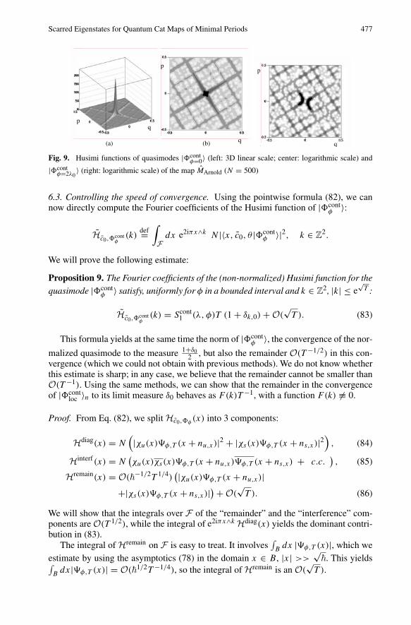
Scarred Eigenstates for Quantum Cat Maps of Minimal Periods 477
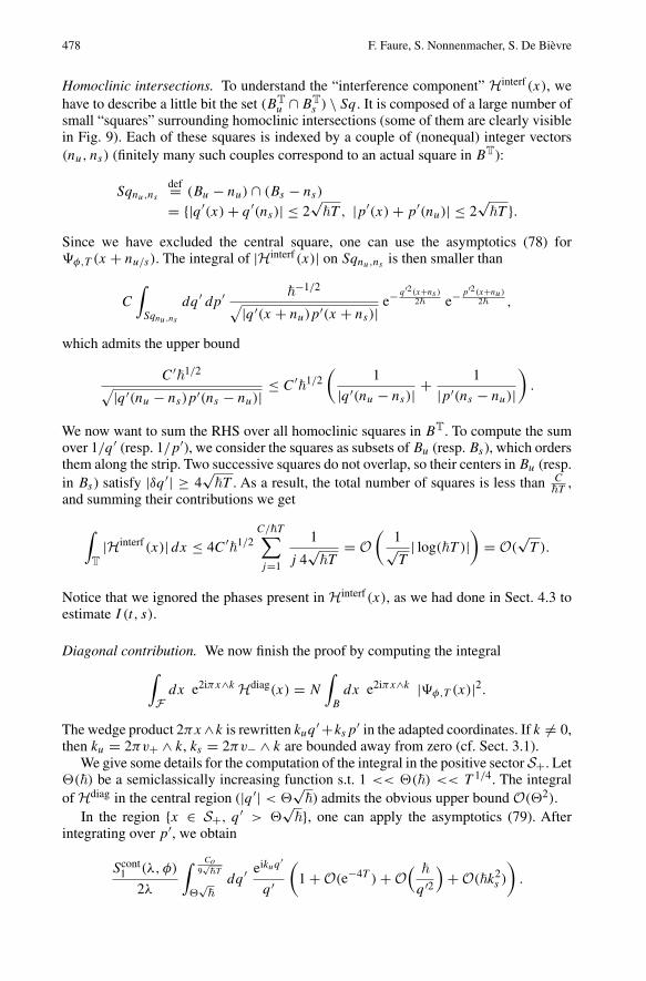
(a) (b)
qp
q
pp
q
Fig. 9. Husimi functions of quasimodes |�contφ=0〉 (left: 3D linear scale; center: logarithmic scale) and
|�contφ=2λ0
〉 (right: logarithmic scale) of the map MArnold (N = 500)
6.3. Controlling the speed of convergence. Using the pointwise formula (82), we cannow directly compute the Fourier coefficients of the Husimi function of |�cont
φ 〉:
Hc0,�contφ(k)
def=∫
Fdx e2iπx∧k N |〈x, c0, θ |�cont
φ 〉|2, k ∈ Z2.
We will prove the following estimate:
Proposition 9. The Fourier coefficients of the (non-normalized) Husimi function for the
quasimode |�contφ 〉 satisfy, uniformly for φ in a bounded interval and k ∈ Z
2, |k| ≤ e√T :
Hc0,�contφ(k) = Scont
1 (λ, φ)T (1+ δk,0)+O(√T ). (83)
This formula yields at the same time the norm of |�contφ 〉, the convergence of the nor-
malized quasimode to the measure 1+δ02 , but also the remainder O(T −1/2) in this con-
vergence (which we could not obtain with previous methods). We do not know whetherthis estimate is sharp; in any case, we believe that the remainder cannot be smaller thanO(T −1). Using the same methods, we can show that the remainder in the convergenceof |�cont
loc 〉n to its limit measure δ0 behaves as F(k)T −1, with a function F(k) �≡ 0.
Proof. From Eq. (82), we split Hc0,�φ (x) into 3 components:
Hdiag(x) = N(|χu(x)�φ,T (x + nu,x)|2 + |χs(x)�φ,T (x + ns,x)|2
), (84)
Hinterf(x) = N(χu(x)χs(x)�φ,T (x + nu,x)�φ,T (x + ns,x) + c.c.
), (85)
Hremain(x) = O(�−1/2T 1/4)(|χu(x)�φ,T (x + nu,x)|
+|χs(x)�φ,T (x + ns,x)|)+O(
√T ). (86)
We will show that the integrals over F of the “remainder” and the “interference” com-ponents are O(T 1/2), while the integral of e2iπx∧k Hdiag(x) yields the dominant contri-bution in (83).
The integral of Hremain on F is easy to treat. It involves∫Bdx |�φ,T (x)|, which we
estimate by using the asymptotics (78) in the domain x ∈ B, |x| >> √�. This yields∫
Bdx|�φ,T (x)| = O(�1/2T −1/4), so the integral of Hremain is an O(√T ).
478 F. Faure, S. Nonnenmacher, S. De Bievre
Homoclinic intersections. To understand the “interference component” Hinterf(x), wehave to describe a little bit the set (BT
u ∩BTs ) \ Sq. It is composed of a large number of
small “squares” surrounding homoclinic intersections (some of them are clearly visiblein Fig. 9). Each of these squares is indexed by a couple of (nonequal) integer vectors(nu, ns) (finitely many such couples correspond to an actual square in BT):
Sqnu,nsdef= (Bu − nu) ∩ (Bs − ns)= {|q ′(x)+ q ′(ns)| ≤ 2
√�T , |p′(x)+ p′(nu)| ≤ 2
√�T }.
Since we have excluded the central square, one can use the asymptotics (78) for�φ,T (x + nu/s). The integral of |Hinterf(x)| on Sqnu,ns is then smaller than
C
∫
Sqnu,ns
dq ′ dp′�−1/2
√|q ′(x + nu)p′(x + ns)|e−
q′2(x+ns )2� e−
p′2(x+nu)2� ,
which admits the upper bound
C′�1/2√|q ′(nu − ns)p′(ns − nu)|
≤ C′�1/2(
1
|q ′(nu − ns)| +1
|p′(ns − nu)|).
We now want to sum the RHS over all homoclinic squares in BT. To compute the sumover 1/q ′ (resp. 1/p′), we consider the squares as subsets of Bu (resp. Bs), which ordersthem along the strip. Two successive squares do not overlap, so their centers in Bu (resp.in Bs) satisfy |δq ′| ≥ 4
√�T . As a result, the total number of squares is less than C
�T,
and summing their contributions we get
∫
T
|Hinterf(x)| dx ≤ 4C′�1/2C/�T∑
j=1
1
j 4√
�T= O
(1√T| log(�T )|
)= O(
√T ).
Notice that we ignored the phases present in Hinterf(x), as we had done in Sect. 4.3 toestimate I (t, s).
Diagonal contribution. We now finish the proof by computing the integral∫
Fdx e2iπx∧k Hdiag(x) = N
∫
B
dx e2iπx∧k |�φ,T (x)|2.
The wedge product 2πx∧k is rewritten kuq ′ +ksp′ in the adapted coordinates. If k �= 0,then ku = 2πv+ ∧ k, ks = 2πv− ∧ k are bounded away from zero (cf. Sect. 3.1).
We give some details for the computation of the integral in the positive sector S+. Let�(�) be a semiclassically increasing function s.t. 1 << �(�) << T 1/4. The integralof Hdiag in the central region (|q ′| < �
√�) admits the obvious upper bound O(�2).
In the region {x ∈ S+, q ′ > �√
�}, one can apply the asymptotics (79). Afterintegrating over p′, we obtain
Scont1 (λ, φ)
2λ
∫ Co
9√
�T
�√
�
dq ′eikuq ′
q ′
(1+O(e−4T )+O
(�
q ′2)+O(�k2
s )
).
Scarred Eigenstates for Quantum Cat Maps of Minimal Periods 479
This integral is easy to estimate:
• for k = 0, it yields
Scont1 (λ, φ)
2λlog
( C
�√T�
)+O(�−2) = Scont
1 (λ, φ)
2T +O( log(�
√T )).
• for k �= 0, it has the asymptotics [BaHTF, Chap. 9]
Scont1 (λ, φ)
2λ| log(
√��ku)| +O(1) = Scont
1 (λ, φ)
4T +O(log(�ku)).
Taking the 3 remaining sectors into account, we obtain the proposition. ��
6.4. Husimi function close to the origin andLs norms. Besides providing the limit semi-classical measure, the pointwise formula (82) allows us to compute different indicatorsof localization for the quasimode |�cont
φ 〉n, namely the Ls norms of its Husimi function[Pr, NV2]:
(s > 0) ‖H�‖s def=(∫
T
[H�(x)]s dx
)1/s
.
For s = 2, this defines a phase space analogy of the “inverse participation ratio” used incondensed-matter physics; in the limit s → 1+, it yields the Wehrl entropy of the state;for s →∞, this is sup-norm of the Husimi density.
Proposition 10. For any fixed ∞ ≥ s > 1 and φ in a bounded interval, the Ls normsof the quasimodes |�cont
φ 〉n behave in the semiclassical limit as
∥∥∥Hc0,|�contφ 〉n
∥∥∥s∼ C(s, φ/λ)
�1− 1
s | log �|.
By comparison, the Ls-norms of a coherent state |c, θ〉 behave as C′(s, c)�−1+1/s as� → 0, c in a bounded set [NV2]. In the case of the sup-norm, we have a more precisestatement (see Fig. 8):
Proposition 11. For small enough �, the maximum of Hc0,|�contφ 〉n(x) is at the origin
for |φ|/λ < 0.5, and C(∞, φ/λ) = |�(1/4+iφ/2λ)|225/2π3/2 . Conversely, for |φ|/λ >> 1,
the maximum is close to the points Q′ = −P ′ = ±√φ/λ on the hyperbola, andC(∞, φ/λ) ∼ (25/2√π |φ|/λ)−1.
Sketch of proof. For any s > 1, the decrease ∼ 1|x|s of the Husimi function along the
hyperbola implies that most of the weight in the integral∫F Hs
�contφ
is supported near the
origin, so that this integral is close to∫R2 Hs
�(even)φ
. This yields the proposition, with the
coefficientsC(s, φ/λ) given as integrals of parabolic cylinder functions. The statementson the maxima derive from known results about parabolic cylinder functions. ��
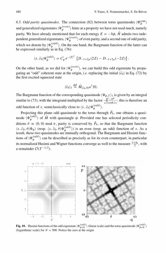
480 F. Faure, S. Nonnenmacher, S. De Bievre
6.5. Odd-parity quasimodes. The connection (82) between torus quasimodes |�contφ 〉
and generalized eigenstates |�(even)φ 〉 hints at a property we have not used much, namely
parity. We have already mentioned that for each energy E = −�φ, H admits two inde-pendent generalized eigenstates, |�(even)φ 〉 of even parity, and a second one of odd parity,
which we denote by |�(odd)φ 〉. On the one hand, the Bargmann function of the latter canbe expressed similarly as in Eq. (76):
〈x, c0|�(odd)φ 〉 = C′φ e−|Z|2{D−1+2µ(2Z)−D−1+2µ(−2Z)
}.
On the other hand, as we did for |�(even)φ 〉, we can build this odd eigenstate by propa-gating an “odd” coherent state at the origin, i.e. replacing the initial |c0〉 in Eq. (72) bythe first excited squeezed state
|c0〉1 def= M(c0,0)a†|0〉.
The Bargmann function of the corresponding quasimode |�φ,T 〉1 is given by an integral
similar to (73), with the integrand multiplied by the factor Q′−iP ′√2 cosh λs
: this is therefore an
odd function of x, semiclassically close to 〈x, c0|�(odd)φ 〉.Projecting this plane odd quasimode to the torus through Pθ , one obtains a quasi-
mode |�(odd)φ 〉 of M with quasiangle φ. Provided one has selected periodicity con-
ditions θ ≡ (0, 0) mod π , parity is conserved by Pθ , so that the Bargmann function〈x, c0, θ |�φ〉 (resp. 〈x, c0, θ |�(odd)φ 〉) is an even (resp. an odd) function of x. As aresult, these two quasimodes are mutually orthogonal. The Bargmann and Husimi func-tions of |�(odd)φ 〉 can be described as precisely as for its even counterpart, in particular
its normalized Husimi and Wigner functions converge as well to the measure 1+δ02 , with
a remainder O(T −1/2).
q
p
Fig. 10. Husimi functions of the odd eigenstate |�(odd)φ=0 〉 (linear scale) and the torus quasimode |�(odd)φ=0 〉(logarithmic scale) for N = 500. Notice the zero at the origin
Scarred Eigenstates for Quantum Cat Maps of Minimal Periods 481
6.6. On the “robustness” of continuous quasimodes. We want to show that the con-tinuous quasimodes |�cont
φ 〉, |�oddφ 〉 are “stable” with respect to a change of the initialstate (|c0〉 and |c0〉1, respectively). One can indeed obtain an even quasimode very closeto |�cont
φ 〉 by propagating a different initial state |ψ0〉: this state needs to be of evenparity, sufficiently localized (e.g. a finite combination of excited coherent states), andtaken away from a subspace of “bad” initial states. These remarks will be made morequantitative in Appendix 10.2, which treats the case where |ψ0〉 is a squeezed coherentstate of arbitrary squeezing.
To explain this “robustness”, we notice that the operator
Pcont−∞,∞,φ
def=∫ ∞
−∞ds e−iφs e−iH s/�
projects L2(R) onto the 2-dimensional space spanned by |�(even)φ 〉 and |�(odd)φ 〉. Any
even state |ψ0〉 ∈ L2(R)will thus be projected ontoCφ(ψ0)|�(even)φ 〉, with the prefactor
Cφ(ψ0) =〈�(even)φ |ψ0〉〈�(even)φ |c0〉
.
This prefactor vanishes iff there exists a state |ϕ0〉∈L2(R) such that |ψ0〉=(H+�φ)|ϕ0〉;such |ψ0〉 form a “bad” subspace of codimension 1 inside the space of even states.
If |ψ0〉 is localized inside a disk of radius C�1/2+ε at the origin, one can describe the
plane quasimode Pcont−T ,T ,φ |ψ0〉 as in (77):
〈x, c0|Pcont−T ,T ,φ |ψ0〉 = Cφ(ψ0)〈x, c0|�(even)φ 〉 +O(�1/2−ε) uniformly in x ∈ R
2.
(87)
If Cφ(ψ0) is of order unity, this estimate shows that Pcont−T ,T ,φ |ψ0〉 resembles the quasi-
mode |�φ,T 〉. One can then show (as in Sect. 6.2) that the torus state Pθ Pcont−T ,T ,φ |ψ0〉 is
close to the quasimode Cφ(ψ0)|�contφ 〉.
As an example, consider the case φ = 0: one can start from any (finitely) excitedcoherent state of the form |c0〉4n ∝ M(c0,0)
(a†)4n|0〉 to obtain a quasimode asymptoti-
cally close to |�cont0 〉. On the opposite, the states |c0〉4n+2 are “bad” initial states, because
they are in the range of H .This discussion straightforwardly transposes to the construction of the odd quasi-
modes |�oddφ 〉 starting from odd localized states.
7. Quasimodes on a General Periodic Orbit
We have so far described the construction of quasimodes localized on the fixed point 0of the classical map M . We will now generalize this construction to a general periodicorbit ofM . The associated Husimi densities will be shown to be (semiclassically) partlylocalized on the orbit and partly equidistributed. The proofs require some minor changeswith respect to the previous case, but no fundamentally new ingredients.
We consider a fixed periodic orbit P = {x� ∈ F}τ�=0 of (primitive) period τ , in otherwords, for 0 ≤ � < τ ,Mx� = x�+1 mod Z
2 and xτ = x0. Note thatMτx� = x� mod Z2,
482 F. Faure, S. Nonnenmacher, S. De Bievre
so that all x�, when viewed as points on the torus, are fixed points of M ′ def= Mτ . Fur-thermore, for all 0 ≤ � ≤ τ , there exist m� ∈ Z
2 so that
x� = M�x0 −m�.We will first introduce the discrete time quasimode defined in (2) and will consider itscontinuous time analog below:
|�discφ 〉 =
T−1∑
t=−Te−iφt Mt Pθ Tx0 |c0〉.
Letting T be the integer multiple of τ that is closest to | ln �|/λ, and setting T ′ = T/τ ,a simple computation yields
|�discφ 〉 =
τ−1∑
�=0
e−iφ� |�disc� 〉 where |�disc
� 〉 = M�
T ′−1∑
k=−T ′e−iφτk M ′k
Pθ Tx0 |c0〉.
(88)
It is easy to see that
M�Pθ Tx0 = Pθ Tx�+m�M� = eiS� Pθ Tx�M
�, (89)
where S� = θ ·ml + iδml + iπNml ∧ xl (see (19)). This phase can partly be interpretedin terms of the action along the classical orbit; however, the θ -term is non-classical,akin to the quantum phase due to a pointwise magnetic flux tube on a charged particle(Aharonov-Bohm effect) [KM]. Hence
|�disc� 〉 = eiS�
T ′−1∑
k=−T ′e−iφτk M ′k
Pθ Tx�M�|c0〉. (90)
This suggests that |�disc� 〉 is a quasimode of quasiangle φτ for M ′, associated to the
fixed point x� of M ′. This is basically the content of Proposition 12. There is anotherinstructive way of rewriting |�disc
� 〉 which corroborates this idea. For that purpose, wefirst draw from Eq. (89),
MτkPθ Tx0 = eikSτ Pθ Tx0Mτk and Mτk+�Pθ Tx0 = ei(kSτ+S�) Pθ Tx�M
τk+�. (91)
Using this, one can write
|�disc� 〉 = eiS� Tx� Pθ�
T ′−1∑
k=−T ′e−i(φτ−Sτ )k M ′k
M�|c0〉, (92)
where we used Pθ Tx� = Tx� Pθ�with θ� = θ + 2πN(p�,−q�). A simple computation
shows that, because x� is a fixed point for Mτ , θ� is a fixed point for the map θ → θ ′defined in (31), with M replaced by M ′. Consequently, |�disc
φ 〉 is the x� translate of
a quasimode for M ′ at the origin with quasiangle φτ − Sτ , of the type studied in theprevious sections.
Scarred Eigenstates for Quantum Cat Maps of Minimal Periods 483
To build continuous time quasimodes, we replace in all the above formulas |c0〉 by
1
τ
∫ τ
0dt e−it φ e−
i�H t |c0〉, (93)
where the “quasienergy” φ ∈ R is chosen so that
τ φ ≡ τφ − Sτ mod 2π. (94)
Whereas the quasiangle φ is defined modulo 2π , the quasienergy φ is chosen in R. Thecontinuous quasimode reads:
|�cont� 〉 = eiS� Tx� Pθ�
1
τ
∫ T
−Tdt e−iφt e−
i�H t M�|c0〉. (95)
All the above quasimodes can of course in obvious ways be split into a localized and anequidistributing part, as before. For both the discrete and continuous time quasimodeswe have the following estimates:
Proposition 12. For all 0 ≤ �′ < � ≤ τ − 1, for all f ∈ C∞0 (T2), for all k ∈ Z,
〈��|��〉 = 2T ′S1(φτ − Sτ , τλ)+O(1), (96)
lim�→0
n〈��|f |��〉n = 1
2f (x�)+ 1
2
∫
T2f (x)dx, (97)
lim�→0
n〈��′ |Tk/N |��〉n = 0. (98)
The quasimodes |�φ〉 satisfy (7), the limit being uniform for φ, φ in a bounded interval.
Starting from (95) a pointwise analysis of the continuous time quasimode |�contP,φ〉
can be performed as well, along the lines of Sect. 6.2. One should notice that the Husimifunction of |�cont
P,φ〉 in the√
�-vicinity of a periodic point xl is dominated by the contri-
bution of |�contl 〉; it is concentrated on a hyperbola which depends on the quasienergy
φ rather than on the quasiangle φ.
Proof of the proposition. We write the proof for the discrete time quasimodes only.Equation (92) immediately implies (96) and (97) as a consequence of the results ofSect. 5. To prove (98) when k = 0, i.e. the asymptotic orthogonality of the |��〉, wewrite, using (88) and (91),
〈�disc�′ |�disc
� 〉
=T ′−1∑
k′=−T ′
T ′−1∑
k=−T ′e−i(φτ−Sτ )(k−k′)+iS�−�′ 〈c0|T−x0 Pθ Tx�−�′ M
(�−�′)+τ(k−k′)|c0〉,
so that
∣∣〈�disc�′ |�disc
� 〉∣∣ ≤T ′−1∑
k′=−T ′
T ′−1∑
k=−T ′
∑
m∈Z2
|〈c0|T−x0 TmTx�−�′ M(�−�′)+τ(k−k′)|c0〉|
≤T ′−1∑
k′=−T ′
T ′−1∑
k=−T ′Jr(τ (k − k′)+ �− �′, 0) ≤ C, (99)
484 F. Faure, S. Nonnenmacher, S. De Bievre
where r = x0 − x�−�′ , and where we used the estimate Jr(t, 0) ≤ C� eλ|t |/2 extractedfrom Appendix 10.1. To prove (98) when k �= 0, one repeats the arguments of Sect. 5:we omit the details. For continuous quasimodes, the proofs are analogous, using thistime the same estimate on Jr(t, s). The proof of (7) follows immediately. ��Convex combinations of limit measures. We can further enlarge the set of semiclassi-cal limit measures by taking finite convex combinations of the previous ones. Considera finite set of periodic orbits {P1, . . . ,Pf }, and complex coefficients {α1, . . . , αf }satisfying
∑fi=1 |αi |2 = 1. Let |�Pi ,φ〉 be quasimodes (discrete or continuous time)
associated to Pi , as defined above, with the same quasiangle φ. We can then combinethem into the quasimode
|�〉 def=f∑
i=1
αi |�Pi ,φ〉n.
One readily shows along the lines of the proof of Proposition 12 that for i �= j , and forall k ∈ Z
2, one haslim�→0
n〈�Pi|Tk/N |�Pj
〉n = 0.
This together with (7) shows that the Husimi and Wigner functions of |�〉n converge to
the limit measure 12
(dx +∑f
i=1 |αi |2 δPi
).
8. Scarred Eigenstates for Quantum Cat Maps of Short Quantum Periods
We will now slightly extend an argument from [BonDB1] in order to show that thequasimodes we have built and studied in the previous sections are exact eigenstates ofthe quantum map M for certain special values of � and we will prove Theorem 1.
For that purpose, we first recall a few facts about quantum cat maps [HB]. For a givenvalue of N = (2π�)−1, every quantum map M has a “quantum period” P(N) definedto be the smallest nonnegative integer such that
MP (N) = eiϕ(N) IHN,θfor a certain ϕ(N) ∈ [−π, π [. (100)
It follows that, if φ is of the type φ = φj = ϕ(N)+2πjP (N)
, then 1P(N)
Pt1,t1+P(N),φj is
independent of t1, and is the spectral projector onto the eigenspace of M inside HN,θ
associated to the eigenvalue eiφj (the normalization factor 1/P (N) ensures that it isindeed a projector). All eigenvalues of M on HN,θ are necessarily of that form.
The function P(N) depends onN in an erratic way, and no closed formula exists forit [Ke]. It satisfies the general bounds
∃C > 0, ∀N ∈ N∗,
2
λlogN − C ≤ P(N) ≤ C N log logN. (101)
It is moreover known that, for “almost all” integers, P(N) ≥ √N [KR2]. We will now
give an elementary argument to show that, given any hyperbolic matrix in SL(2,Z),there exists an infinite sequence of integers Nk for which the quantum period is veryshort in the sense that it saturates the above lower bound:
P(Nk) = 2logNkλ
+O(1) = 2Tk +O(1), (102)
where the Ehrenfest time T was defined in (45).
Scarred Eigenstates for Quantum Cat Maps of Minimal Periods 485
Let us first recall that, for all k ∈ N∗, one has
Mk = pkM − pk−1, where pk =eλk − e−λk
eλ− e−λ, p0 = 0.
It was proven in [BonDB1] that, for all k ≥ 1, the integer Nk = GCD(pk, pk−1 + 1)satisfies
2
λlog Nk = k +O(1), (103)
and that
Mk = I + NkMk, with Mk an integer matrix. (104)
We now set Nk = Nk if Nk is odd, Nk = Nk/2 if Nk is even. Choosing the periodicityangle θ = (0, 0) when Nk is even and θ = (π, π) when Nk is odd (which makes sense,cf. the end of Sect. 3.2), we prove below the following lemma:
Lemma 4. With Nk , θ given as above, Mk = eiϕ IHNk,θfor a certain ϕ ∈ [−π, π [.
This means that the quantum period P(Nk) of M on HNk,θ divides k. Comparing(101) with (103) entails that for k large enough, P(Nk) = k and (102) holds.
Proof of the lemma. The case Nk = 2Nk , θ = (0, 0) was treated in [HB]. We give adifferent proof, which works for both cases.
From Schur’s Lemma and the irreducibility of the Tn/Nk , it suffices to show that[Mk, Tn/Nk
]= 0 on HNk,θ , for all n ∈ Z
2. Setting Nk = εNk , θ = ε′(π, π) and using
the definition of Pθ , Eqs. (19) and (20), one readily computes
MkTn/Nk M−kPθ = eiπε(n∧Mkn) Tn/Nk TMknPθ
= (−1)ε(n∧Mkn)+εε′[(Mkn)1+(Mkn)2+(Mkn)1(Mkn)2]Tn/Nk Pθ .
This phase is trivial if ε = 2. In the case ε = ε′ = 1 (that is, Nk odd), one must considerthe 6 possible values of M modulo 2: in all cases, the phase is trivial. ��
If we now consider such a value Nk together with an admissible eigenangle φjk , theeigenstates
|�k〉 =P(Nk)/2−1∑
t=−P(Nk)/2e−iφjk t Mt |x0, c0〉
are (discrete time) quasimodes of the quantum map as studied in the previous sections.Indeed, as discussed at the end of Sect. 5, since T and P(Nk)/2 differ by a boundednumber of terms in the semiclassical limit, we can replace one by the other in (2), with-out affecting any of the semiclassical properties of the quasimodes. One can similarlyconstruct eigenfunctions that are continuous time quasimodes.
486 F. Faure, S. Nonnenmacher, S. De Bievre
Proof of Theorem 1. The previous arguments settle the case β = 1/2. To treat the gen-eral case, we recall that the Schnirelman theorem implies the existence of a sequenceof eigenfunctions |ϕk〉n of M on HNk,θ (with corresponding eigenvalues (φjk )k∈N) thatequidistribute as k→∞. We then construct, for 0 ≤ α ≤ 1:
|ψk〉 = α|�k〉n +√
1− α2|ϕk〉n.If we show that, for all n ∈ Z
2,
lim�→0
n〈ϕk|Tn/Nk |�k〉n = 0,
a simple computation implies that the |ψk〉n satisfy (8) with β = α2/2. We have
lim�→0
n〈ϕk|Tn/Nk |�k〉n = lim�→0
(n〈ϕk|Tn/Nk |�k,erg〉n + n〈ϕk|Tn/Nk |�k,loc〉n
).
The second limit vanishes with an argument as in (71), whereas for the first, we use thefurther decomposition |�k,erg〉 = |�k,1〉 + |�k,4〉 with |�k,1〉 = eiφjk T /2 M−T/2|�k,2〉,|�k,4〉 = e−iφjk T /2 MT/2|�k,3〉 (see (3)). Now, since |ϕjk 〉n is an eigenfunction, we have
∣∣n〈ϕk|Tn/Nk |�k,4〉n
∣∣ = ∣∣n〈ϕk|M−T/2Tn/Nk M
T/2|�k,3〉n∣∣.
As in the proof of Proposition 6, and more specifically Eq. (71), this tends to 0 with �.��
For matrices M of “checkerboard structure”, the results of [KR1, Me] imply that,given an arbitrary sequence of eigenvalues (φjk )k∈N, there exists a corresponding se-quence of eigenvectors |ϕk〉 ∈ HNk,θ that semiclassically equidistribute. One can thenconstruct for the same eigenvalues eigenstates |ψk〉 satisfying Eq. (8).
The P(Nk) eigenstates with distinct eigenvalues constructed above are of courseexactly orthogonal to each other, and not just asymptotically as proven in Sect. 5.3. Onthe other hand, two continuous time eigenstates of identical eigenangle φj but differentquasienergies φ − φ′ = sπ/T , s �= 0 become orthogonal in the semiclassical limit.This is also the case for two eigenstates with the same eigenangle supported on differentperiodic orbits P �= P ′.
9. Conclusion
In this article we have constructed and analyzed a certain class of “quasimodes” ofhyperbolic quantized torus isomorphisms, which for certain values of � become exacteigenstates. The characteristic property of these quasimodes is that their “quantum limit”,that is the weak limit of their Husimi densities, does not yield the Liouville measure,but contains a singular component supported on a (finite union of) periodic orbit(s). Inour case, this singular component has a relative weight β ≤ 1/2, less than or equalto the weight of the Liouville part. As explained in the introduction, no limit measureof eigenstates can have a “larger” singular component. We further conjecture that nosequence of quasimodes (i.e. images of the operators ∧P−T ,T ,φ) can have a more singularlimit measure either.
The strong scarring of eigenstates exhibited in this paper is directly linked to thevery large degeneracies of the eigenvalues of M for certain special values of Planck’s
Scarred Eigenstates for Quantum Cat Maps of Minimal Periods 487
constant. Therefore, such sequences of eigenstates are very probably absent as soon as
one considers nonlinear perturbations of the dynamics, for instance Mε = e−iεH1/� M ,for any periodic HamiltonianH1(x) and ε > 0 small enough. Such a perturbation of theclassical map is known to conserve the uniform hyperbolicity, but destroys the “actiondegeneracies” characteristic of the (linear) cat map. As a consequence the spectrum ofthe perturbed map exhibits Random Matrix statistics, in particular “repulsion” betweeneigenangles [KM], which forbids degeneracies.
The precise characterization of some weaker form of scarring for individual eigen-states that would remain valid for Mε remains therefore an open problem. Nevertheless,it might be interesting to study the phase space distribution of the “nonlinear“ quasi-modes of the type
∑Tt=−T e−iφt Mt
ε |x0, c〉, for x0 a periodic point ofMε , which may notbe as simple to describe as for the linear map.
Acknowledgements. We have benefited from useful conversations with Y. Colin de Verdiere, C. Gerard,E. Vergini, A. Voros, D. Wisniacki. F. F. acknowledges the kind hospitality of the Service de PhysiqueTheorique, CEA Saclay where part of this work was accomplished.
10. Appendices
10.1. Estimate of the interference term I (t, s). In this appendix we prove Proposition 1.For the purpose of Sect. 7 we will at the same time give a bound for the more generaloverlap (t, s ∈ R)
∣∣∣〈r, cs |Pθ e−iH t/� |cs〉∣∣∣ ≤
∑
n∈Z2
∣∣∣〈r + n, cs | e− i�H t |cs〉
∣∣∣ , (105)
where r ∈ F (the fundamental domain) belongs to the lattice( 1D
Z)2
, with D ∈ N∗ and
where θ ∈ [0, 2π [×[0, 2π [ is arbitrary (in other words, θ need not be equal to the fixedpoint of the map (31). We define
Jr(t, s)def=
∑
n∈Z2,r+n�=0
∣∣∣〈r + n, cs | e− i�H t |cs〉
∣∣∣ . (106)
We first consider the case s = 0, t ≥ 0. Since√
� ≤ �p′ ≤ √2� for all positive times,
only the points r + n near the unstable axis can significantly contribute. Therefore, wesubdivide the plane into strips parallel to this axis: the “outer” strips
∀l ≥ 1, S±l ={x | al ≤ ±p′(x) < al+1
},
with al = W0+(l−1)W , and the central strip S0 ={x �= 0 | p′(x)| < W0
}. The widths
W0, W will be explicitly set below.We start by estimating the contribution of the points r + n ∈ Sl with l ≥ 1. Due to
the diophantine condition (25), as long as W is small enough, two points in this stripsatisfy the property |q ′(r + n)− q ′(r +m)| > Co/W . Ordering these points accordingto their abscissas: q ′(r + nj ) < q ′(r + nj+1) < q ′(r + nj+2), we have for any α > 0 :
∑
j∈Z
exp{−αq ′(r + nj )2
}≤∑
j∈Z
exp
{−α
(jCo
W
)2}. (107)
488 F. Faure, S. Nonnenmacher, S. De Bievre
The sum on the RHS is a one-dimensional theta function, which has the upper bound(optimal for 0 < α small enough):
∑
j∈Z
e−αj2 ≤ 1+√π
α. (108)
As a result, using (43) it becomes clear that the contribution to Jr(t) of the pointsr + n ∈ Sl is bounded above by
∑
r+nj∈Sl
1√cosh λt
exp
{−1
2
[p′(r + nj )2�p′2
+ q ′(r + nj )2�q ′2
]}
≤√
2 e−λt/2 e− a2
l
2�p′2[
1+√
2πW�q ′
Co
]. (109)
The estimate (108) can then be applied to the sum over the strips Sl , l �= 0, to obtain
(remind |t; c0〉 = e−iH t/� |c0〉)∑
l �=0
∑
r+n∈Sl|〈r + n, c0|t; c0〉|
≤√
2 e−λt/2 e− W2
02�p′2
[2+
√2π�p′
W
] [1+
√2πW�q ′
Co
].
For each time t , we can minimize the RHS with respect toW by takingW 2 = Co�p′
2�q ′ =Co2 e−λt , which leads to the bound
∑
l �=0
∑
r+n∈Sl|〈r + n, c0|t; c0〉| ≤ 2
√2 e
− W20
2�p′2 e−λt/2[
1+√π
Co�p′ eλt/2
]2
. (110)
Notice that this upper bound is independent of the point r .We now estimate the contribution of the strip S0, which requires more care, and will
depend on r . For any point r ′ �= 0 on the lattice( 1D
Z)2
sufficiently close to the unstable
axis, the diophantine property (25) implies |p′(r ′)| ≥ CoD2|q ′(r ′)| . As a consequence, the
quadratic form appearing in (43) may be bounded inside S0 by
q ′(r + n)22�q ′2
+ p′(r + n)22�p′2
≥ q ′(r + n)22�q ′2
+ C2o
2D4�p′2 q ′(r + n)2def= ft (q
′(r + n)).(111)
The function ft satisfies the scaling property ft (q) = Co e−λt2D2�p′2 f
(qD e−λt/2√
Co
), with
f (q)def= q2 + q−2. This function f (q) is bounded below for all positive q by the
parabola g(q) = 2+ (q − 1)2, so after rescaling we get
∀q > 0, ft (q) ≥ gt (q) def= Co e−λt
D2�p′2+ e−2λt
2�p′2(q −
√Co eλt/2 /D
)2.
Scarred Eigenstates for Quantum Cat Maps of Minimal Periods 489
We consider the contributions of the points r+n in S0 such that q ′(r+n) > 0 (the pointswith negative q ′ can be treated identically). We order these points as 0 < q ′0 < q ′1 < . . . :
each contribution is bounded above by the quantity (cosh λt)−1/2 e−gt (q′j ), which is max-
imal for the q ′j close to√Co eλt/2 /D. The diophantine inequality |q ′j −q ′j+1| ≥ Co/W0
together with the estimates (107,108) then yield
∑
r+n∈S0
|〈r + n, c0|t; c0〉| ≤ 2√
2 exp
{− Co e−λt
D2�p′2
}e−λt/2
(1+
√2πW0�p
′ eλt
Co
).
(112)
This contribution now depends on the rational point r through its denominator D: theupper bound increases with D. The full sum Jr(t) is bounded above by the sum of theRHS in (110)–(112). For each time t , we adjust the value ofW0 to minimize that sum. Wedo not search the exact minimum, but only its order of magnitude. We have to distinguishtwo time intervals:
• for short times (t << T ), the behaviour of (112) is governed by the first exponen-tial (since �p′2 ≤ 2�). We take W0 such that the first exponential in (110) is muchsmaller than that factor, for instance by takingW0 = 2
√Co e−λt/2 /D. Being careful
for times around t � T , we find
0 ≤ t ≤ T �⇒ Jr(t, 0) ≤ 2√
2 exp
{− Co e−λt
D2�p′2(t)
}e−λt/2
[1+ C eλ(t−T )/2
],
where the constantC is independent on the denominatorD. One may replace�p′2(t)by its maximum 2� for positive times. The RHS increases with the denominator D.
• for times t ≥ T , the RHS of (112) is now governed by the factor between brackets,and we want to make sure that (110) is not larger than it. Still taking W0 = e−λt/2leads to the estimate:
T ≤ t ≤ 2T �⇒ Jr(t, 0) ≤ 2π√
2
Co� eλt/2
[1+ C′ eλ(T−t)/2
].
The constant C′ is independent of r , so this bound applies uniformly to any pointx ∈ T: it yields aL∞-bound for the Bargmann (or the Husimi) function of Mt |c0, θ〉.
The same bounds apply as well to Jr(t, s) with s �= 0. Indeed, replacing the initialsqueezing c0 by its s-evolved value amounts to dilating the coordinates of the points asq ′(r + n) �→ eλt1 q ′(r + n), p′(r + n) �→ e−λt1 p′(r + n). One easily checks that thisdilation does not modify the above bounds.
The negative times are treated thanks to the identity Jr(t, s) = J−M−t r (−t, s), andnoticing that the above bounds only depend on the denominator D, common to r andM−t r .
10.2. Changing the initial squeezing. We chose from the beginning to construct quasi-modes starting from the coherent state |c0〉 defined in Sect. 4.2. The definition wasmotivated by the positivity property (40) of the overlap 〈c0|Mt |c0〉, and by choosing the“smallest” parameter c sharing this property. The simple expression (40) was then usedto control the “interferences” I (t, s) (cf. Appendix 10.1), and to obtain from there the
490 F. Faure, S. Nonnenmacher, S. De Bievre
asymptotic norm of the quasimode (Sect. 5.2), a crucial step for further estimates. Sim-ilarly, we also chose to analyze the quasimodes using the c0-Bargmann representation,because of the relatively simple formulas for 〈x, c0|Mt |c0〉 (see (43)).
We want to stress (as we did in Sect. 6.6 for the continuous quasimodes) that boththese choices were made purely for convenience, and are not crucial for the results of thispaper. The construction of quasimodes can be extended in many ways. In this appendix,we will consider discrete or continuous quasimodes starting from a squeezed state |c1〉,with an arbitrary (possibly �-dependent) squeezing c1. We also want to analyze thesequasimodes using the Bargmann function 〈x, c2, θ |�〉 for some c2 ∈ C which coulddepend on � as well.
Proposition 13. The convergence (7) holds the above quasimodes, as long as c1 and c2stay in a fixed compact set K ⊂ C for all �.
Sketch of proof. For an initial state |c1〉, the overlap 〈x, c1| e−itH /� |c1〉, crucial in thecalculation of I (t, s), is still given by closed formulas. We only give it for the simplercase x = 0:
〈c1| e−itH /� |c1〉 = 〈c′1|D(λt)|c′1〉 =(
cosh(λt)+ iR(c′1) sinh(λt))−1/2
,
where |c′1〉 ∝ Q−1|c1〉 and R(c) = −#(c) sinh(2|c|)2|c| . In general, this overlap is therefore
not real. However, it still decreases exponentially fast with time, and its average
S1(c1, λ, φ) =∫
R
dt e−iφt 〈c1| e−itH /� |c1〉
can be easily related with S1(λ, φ) through a change of variable. One gets S1(c1, λ, φ) =e−φτ1
√cos(λτ1) S1(λ, φ) with the “complex time” τ1 = arctan{R(c′1)}/λ.
For x �= 0, the expression for 〈x, c1|Mt |c1〉 is more cumbersome than (43). Yet,it is still a Gaussian having an elliptic profile of width ∼ √
�, length ∼ √� eλ|t | and
height ∼ e−λ|t |/2, and its long axis is asymptotically lined up with the unstable direc-tion for t → ∞. As a result, the results of Sects. 4.3–5.3 still hold (replacing S1(λ, φ)
by S1(c1, λ, φ)). The localization property (65) holds as well, even if one replaces inthe bras c0 by c2, as long as c2 remains bounded. The rest of the proof to obtain (7)(Sects. 5.5–5.6) goes through unaltered. ��
Following Sect. 6.6, the plane quasimode Pcont−T ,T ,φ |c1〉 can be analyzed pointwise
through the estimate (87); one now has explicitly Cφ(|c1〉) = e−φτ1√
cos(λτ1). Onemay replace c0 by c2 in that estimate. As opposed to Eq. (76), the Bargmann function〈x, c2|�(even)φ 〉 is not given in terms of cylinder parabolic functions. Yet, its behaviour“far” from the origin will be similar to (78). As a consequence, the pointwise estimate(82) (with c0 → c2 in the bras) will apply to the torus quasimode Pθ Pcont
−T ,T ,φ |c1〉 aswell, upon taking the prefactor Cφ(|c1〉) into account and replacing in the bras c0 → c2on both sides. The estimates of Sects. 6.3–6.4 may be generalized as well to the presentcase.
Scarred Eigenstates for Quantum Cat Maps of Minimal Periods 491
References
[AA] Arnold,V.I.,Avez,A.: Ergodic Problems in Classical Mechanics. NewYork: Benjamin, 1968[BaTIT] Tables of integral transforms. A. Erdelyi (ed), New York: Mc-Graw-Hill, 1954[BaHTF] Higher transcendental functions. A. Erdelyi (ed), New York: McGraw-Hill, 1953[Bog] Bogomolny, E.B.: Smoothed wave functions of chaotic quantum systems. Physica 31 D,
169–189 (1988)[Ber] Berry, M.V.: Quantum scars of classical closed orbits in phase space. Proc. R. Soc. Lond. A
423, 219–231 (1989)[BonDB1] Bonechi, F., De Bievre, S.: Exponential mixing and ln � timescales in quantized hyperbolic
maps on the torus. Commun. Math. Phys. 211, 659–686 (2000)[BonDB2] Bonechi, F., De Bievre, S.: Controlling strong scarring for quantized ergodic toral automor-
phisms. Duke Math. J. 117, 571–587 (2003)[BouDB] Bouzouina, A., De Bievre, S.: Equipartition of the eigenfunctions of quantized ergodic maps
on the torus. Commun. Math. Phys. 178, 83–105 (1996)[CKS] Chang, C.-H., Kruger, T., Schubert, R.: Quantizations of piecewise affine maps on the torus
and their quantum limits. In preparation[CdV] Colin de Verdiere, Y.: Ergodicite et fonctions propres du Laplacien. Commun. Math. Phys.
102, 497–502 (1985)[DE] Degli Esposti, M.: Quantization of the orientation preserving automorphisms of the torus.
Ann. Inst. Henri Poincare 58, 323–341 (1993)[DEGI] Degli Esposti, M., Graffi, S., Isola, S.: Stochastic properties of the quantum Arnold cat in
the classical limit. Commun. Math. Phys. 167, 471–509 (1995)[FN1] Faure, F., Nonnenmacher, S.: On the maximal scarring for quantum cat map eigenstates.
To be published[FN2] Faure, F., Nonnenmacher, S.: In preparation[F] Folland, G.: Harmonic analysis in phase space. Princeton NJ: Princeton University Press,
1988[HB] Hannay, J.H., Berry, M.V.: Quantization of linear maps-Fresnel diffraction by a periodic
grating. Physica D 1, 267–290 (1980)[He] Heller, E.J.: Bound-state eigenfunctions of classically chaotic hamiltonian systems: scars of
periodic orbits. Phys. Rev. Lett. 53, 1515–1518 (1984)[HMR] Helffer, B., Martinez, A., Robert, D.: Ergodicite et limite semi-classique. Commun. Math.
Phys 109, 313–326 (1987)[KH] Kaplan, L., Heller, E.J.: Measuring scars of periodic orbits. Phys. Rev. E 59, 6609–6628
(1999)[Ke] Keating, J.P.: Asymptotic properties of the periodic orbits of the cat maps. Nonlinearity 4,
277–307 (1990)[KM] Keating, J.P., Mezzadri, F.: Pseudo-symmetries of Anosov maps and Spectral statistics.
Nonlinearity 13, 747–775 (2000)[Kh] Khinchin, A.: Continued Fractions. Chicago and London: The University of Chicago Press,
1964[KR1] Kurlberg, P., Rudnick, Z.: Hecke theory and equidistribution for the quantization of linear
maps of the torus. Duke Math. J. 103, 47–77 (2000)[KR2] Kurlberg, P., Rudnick, Z.: On quantum ergodicity for linear maps of the torus. Commun.
Math. Phys. 222, 201–227 (2001)[Me] Mezzadri, F.: On the multiplicativity of quantum cat maps. Nonlinearity 15, 905–922 (2002)[NV1] Nonnenmacher, S., Voros, A.: Eigenstate structures around a hyperbolic point. J. Phys. A 30,
295–315 (1997)[NV2] Nonnenmacher, S., Voros, A.: Chaotic Eigenfunctions in Phase Space. J. Stat. Phys. 92,
431–518 (1998)[dPBB] de Polavieja, G.G., Borondo, F., Benito, R.M.: Phys. Rev. Lett. 73, 1613–1616 (1994)[Pe] Perelomov, A.: Generalized coherent states and their applications. Berlin: Springer-Verlag,
1986[Pr] Prosen, T.: Quantum surface of section method: eigenstates and unitary quantum Poincare
evolution. Physica D 91, 244–277 (1996)[ROdA] Rivas, A.M.F., Ozorio de Almeida, A.M.: Hyperbolic scar patterns in phase space.
Nonlinearity 15, 681–693 (2002)[RS] Rudnick, Z., Sarnak, P.: The behaviour of eigenstates of arithmetic hyperbolic manifolds.
Commun. Math. Phys. 161, 195–213 (1994)[Sc] Schnirelman,A.: Ergodic properties of eigenfunctions. Usp. Math. Nauk 29, 181–182 (1974)[WBVB] Wisniacki, D.A., Borondo, F., Vergini, E., Benito, R.M.: Localization properties of groups
of eigenstates in chaotic systems. Phys. Rev. E 63, 066220 (2001)
492 F. Faure, S. Nonnenmacher, S. De Bievre
[Z1] Zelditch, S.: Uniform distribution of the eigenfunctions on compact hyperbolic surfaces.Duke Math. J 55, 919–941 (1987)
[Z] Zhang, W.-M., Feng, D.H., Gilmore, R.: Coherent states: Theory and some applications.Rev. Mod. Phys. 62, 867–927 (1990)
Communicated by P. Sarnak