Draft version June 22, 2021Preprint typeset using LATEX style emulateapj v. 8/13/10

MAGNETIC PAIR CREATION TRANSPARENCY IN GAMMA-RAY PULSARS

Sarah A. Story and Matthew G. BaringDepartment of Physics and Astronomy, MS 108,

Rice University, Houston, TX 77251, U.S.A.ss16@rice.edu, baring@rice.edu

Draft version June 22, 2021

ABSTRACT

Magnetic pair creation, γ → e+e− , has been at the core of radio pulsar paradigms and central topolar cap models of gamma-ray pulsars for over three decades. The Fermi gamma-ray pulsar popula-tion now exceeds 140 sources and has defined an important part of Fermi’s science legacy, providingrich information for the interpretation of young energetic pulsars and old millisecond pulsars. Amongthe population characteristics well established is the common occurrence of exponential turnovers intheir spectra in the 1–10 GeV range. These turnovers are too gradual to arise from magnetic paircreation in the strong magnetic fields of pulsar inner magnetospheres. By demanding insignificantphoton attenuation precipitated by such single-photon pair creation, the energies of these turnoversfor Fermi pulsars can be used to compute lower bounds for the typical altitude of GeV band emission.This paper explores such pair transparency constraints below the turnover energy, and updates earlieraltitude bound determinations of that have been deployed in various Fermi pulsar papers. For lowaltitude emission locales, general relativistic influences are found to be important, increasing cumula-tive opacity, shortening the photon attenuation lengths, and also reducing the maximum energy thatpermits escape of photons from a neutron star magnetosphere. Rotational aberration influences arealso explored, and are found to be small at low altitudes, except near the magnetic pole. The analysispresented in this paper clearly demonstrates that including near-threshold physics in the pair creationrate is essential to deriving accurate attenuation lengths and escape energies. The altitude boundsare typically in the range of 2-7 stellar radii for the young Fermi pulsar population, and provide keyinformation on the emission altitude in radio quiet pulsars that do not possess double-peaked pulseprofiles. The bound for the Crab pulsar is at a much higher altitude, with the putative detection byMAGIC out to 350–400 GeV implying a lower bound of 310km to the emission region, i.e., approx-imately 20% of the light cylinder radius. These results are also extended to the super-critical fielddomain, where it is found that emission in magnetars originating below around 10 stellar radii willnot appear in the Fermi-LAT band.Subject headings: radiation mechanisms: non-thermal — magnetic fields — stars: neutron — pulsars:

general — gamma-rays: theory

1. INTRODUCTION

The Fermi Gamma-ray Space Telescope has revolutionized our understanding of high-energy emission from pulsars.Prior to the launch of Fermi, there were only 7 high-confidence detections (Thompson et al. 1997) of gamma-raypulsars from the EGRET telescope aboard the Compton Gamma-ray Observatory (CGRO), of which all but Gemingahad a radio counterpart. Except for Geminga, which is extremely bright, EGRET was not sensitive enough to performblind searches, the process of discerning pulsation in pulsars using their gamma-ray data alone, i.e. without the guideof an existing radio ephemeris. Furthermore, the maximum observed photon energy, typically in the range 1–10 GeV,was just outside the upper end of EGRET’s sensitive energy range. With the launch of Fermi, a wealth of new databecame available. In just five years, the gamma-ray pulsar sample increased from 7 to over 120 pulsars (Abdo et al.2013, lists 117 in the second Fermi-LAT pulsar catalog), including over three dozen millisecond pulsars and over 35pulsars discovered in Fermi blind searches (Abdo et al. 2009a, 2010a; Saz Parkinson et al. 2010; Abdo et al. 2013).The overwhelming majority of these blind search pulsars have been shown to have no discernible radio counterparts,with upper limits to fluxes at the 30µ Jy level (Abdo et al. 2013). Fermi’s increased sensitivity allows the detection offainter pulsars, and this combined with better time resolution has given us more detailed pulse shapes than EGRETcould provide. The energy window centered on a few GeV is now easily observable for the first time. This has yieldedclear observations of spectral cutoffs and determinations of their shapes in the vast majority of pulsars of all classes: oldmillisecond ones, young radio-quiet and young radio-loud rotators. Such revelations have made it possible to resolvesome long-standing questions about the origins of pulsar high-energy emission.

Prior to the launch of Fermi, there were two competing predictions for the shape of the pulsar spectral cutoff.Outer gap models, driven by curvature radiation physics, predicted a simple exponential cutoff (see, for example,Chiang & Romani 1994), corresponding to the emission by electrons possessing a maximum Lorentz factor. A similarpicture exists for slot gap models (Muslimov & Harding 2004) that extend polar cap-driven emission to high altitudes.In contrast, polar cap models (Daugherty & Harding 1996) based on low altitude photon emission, magnetic paircreation γ → e+e− and pair cascading predict a super-exponential cutoff due to the very strong dependence of thepair production rate on photon energy. EGRET data were equally consistent with either cutoff scenario (Razzano &

arX

iv:1

406.

2767

v1 [

astr

o-ph

.HE

] 1

1 Ju

n 20

14

2

Harding 2007). With far greater statistics, early Fermi-LAT observations of the Vela pulsar clearly exhibited a simpleexponential cutoff (Abdo et al. 2009b), and subsequent observations of Vela and other pulsars have corroborated thisshape, demonstrating that exponential cutoffs are present in the phase-resolved spectroscopic data (Abdo et al. 2010b).Super-exponential spectral turnovers in Fermi GeV band data can be ruled out to high degrees of significance. Thisfact can be used to place a physical lower bound on the altitude of origin for the high-energy emission. The magneticpair creation process is strongly height-dependent and should dominate at low altitudes. Since the signature of strongpair creation - a super-exponential cutoff in the spectrum - is not observed, the emission altitude must be high enoughthat attenuation due to single-photon pair production is not expected.

Even though magnetic pair creation-driven cutoffs do not occur in the Fermi pulsar sample, performing calculationsof magnetic pair production transparency is still a worthwhile exercise. The associated physical lower bounds for theemission height should be considered as a complement to geometric determinations of the emission height from gamma-ray and gamma-ray/radio peak separation in caustic scenarios (Watters et al. 2009; Pierbattista et al. 2010; Venter,Johnson & Harding 2012). In particular, magnetic pair creation altitude bounds can help constrain magnetosphericgeometry in pulsars that do not possess two distinct gamma-ray peaks (about 30% of the blind search pulsars: SazParkinson et al. 2010) and are radio quiet; such pulsars are not as easily amenable to altitude diagnostics using causticgeometry analysis. Furthermore, pair production rates stemming from opacity computations are important for theunderstanding of pulsar wind nebula energetics. The Goldreich-Julian currents alone cannot carry enough energy toaccount for PWN luminosities (Rees & Gunn 1974; de Jager 2007; Bucciantini, Arons & Amato 2011), and to achievethe required energy deposition, there must be prolific pair creation occurring in the pulsar magnetosphere. Single-photon magnetic pair creation is very efficient at low altitudes and can produce large pair multiplicities (Daugherty &Harding 1982; Muslimov & Harding 2003) approaching, but still somewhat lower than, those needed to achieve therequired nebular energy deposition.

Pair opacity calculations date from early pulsar theory, such as in the work of Arons & Scharlemann (1979). Ho,Epstein, & Fenimore (1990), working on early gamma-ray burst theory, recognized that γ − B attenuation posed amajor problem for the escape of gamma-rays from the neutron star surface. Their calculations, which ignored generalrelativistic (GR) and aberration effects, showed that for the escape probability to be significant at soft gamma-rayenergies, emission must be strongly collimated around the local magnetic field. For the higher-energy gamma-raysseen by Fermi, relativistic beaming guarantees that photons will be emitted essentially parallel to the local magneticfield. In Harding, Baring & Gonthier (1997), although the focus was on photon splitting, the authors carried outsingle-photon pair production attenuation calculations for comparison purposes. These calculations included detailedconsideration of threshold effects in the computation of photon attenuation lengths and escape energies, the latterdefining the critical energies above which the magnetosphere is opaque to photon passage for a given emission locale.In an extension of this analysis, Baring & Harding (2001) illustrated the character of magnetic pair creation andphoton splitting opacities by exploring the dependence of photon escape energy on the colatitude of emission for eachprocess, for photons originating at the neutron star surface. They also discussed cascading and the conditions underwhich pair creation (and therefore, arguably, radio emission) should be effectively quenched. Most recently, Lee et al.(2010) tackled the problem of γ − B attenuation in detail. Their work, which produced lower bounds for emissionaltitudes as a function of photon energy, incorporated potentially critical aberration and GR corrections, but largelyignored the threshold behavior of the γ → e+e− rate.

The physics that determines the form of the γ − B attenuation coefficient is discussed in some detail in Section 2.An early offering that described this first-order QED process in a manageable form was in the seminal work by Erber(1966), which provided a simple asymptotic form of the attenuation coefficient. Tsai & Erber (1974) subsequently dealtin detail with the differences in photon polarization modes. Near the pair creation threshold, the simple asymptoticapproximations obtained in these works become less accurate, differing on average by over two orders of magnitudefrom exact pair production rates in fields below around 4 TeraGauss. Daugherty & Harding (1983) provided anempirical approximation to threshold behavior, while formally precise forms were offered in the works of Baring (1988)and Baier & Katkov (2007); none of these is quite as simple as the form highlighted in Erber (1966). These thresholdcorrections are important to address in pair opacity computations involving regions near the stellar surface, when thelocal field is near-critical or higher, i.e. especially for magnetars.

In this work, we have taken an analytical approach to the problem of pair creation opacity whenever possible. Wepresent magnetic pair creation transparency conditions as a function of colatitude and height of emission for photonsemitted parallel to the local magnetic field, as is approximately the case for curvature emission. Our integrals for themagnetic pair creation optical depth are computed for a variety of photon energies and surface polar magnetic fieldsBp . We have included, analytically where possible, corrections for threshold conditions on magnetic pair creation,gravitational redshift, general relativistic magnetic field distortion, and aberration due to neutron star rotation. InSection 3 it is found that in flat spacetime, the maximum energy εesc of a photon that can escape the magnetosphereis a declining function of the emission colatitude θE and the field Bp . In particular, for Bp < 4 × 1012 Gauss, therelationship εescBp sin θE ∼ constant is borne out, in agreement with Arons & Scharlemann (1979) and Chang,Chen, & Ho (1996), a direct consequence of the asymptotic form (Erber 1966) of the pair production rate. When thesurface polar field exceeds around Bp ∼ 1013 Gauss, the threshold influences become profound, and the dependenceof εesc on Bp weakens substantially. If one fixes the escape energy, the altitude at which a photon can be emittedand emerge from the magnetosphere unscathed by magnetic pair attenuation is a monotonically increasing function ofcolatitude θE .

3

Including general relativity effects (see Section 4) reduces the attenuation length for pair creation, lowers the escapeenergies for surface emission locales by 20–30% for Bp < 4 × 1012 Gauss (and around a factor of two for Bp ∼4 × 1013 Gauss) and raises the minimum altitudes of emission by at most 10–20%. For emission points above twostellar radii, GR influences are generally insignificant. Including aberration effects (see Section 5) dramatically raisesthe minimum altitudes rmin for pair transparency at small colatitudes above the magnetic pole. For most emissionazimuthal angles, the minimum altitude of emission increases monotonically with colatitude. In addition, rmin quicklymaps over to the flat spacetime, non-rotating magnetosphere results when θE & 10 — then aberration influences arelargely minimal in the inner magnetosphere because the co-rotation speeds are far inferior to c . This monotonic trendfor rmin continues right up to above the magnetic equator, because of the relative ease with which photons cross fieldlines when propagating at high magnetic colatitudes. In particular, we do not reproduce the putative decline of rmin

as θE approaches 90 that is claimed in Lee et al. (2010), and attributed therein to the influences of aberration.Our pair transparency computations determine that the emission altitude lower bounds calculated for Fermi-LAT

pulsars are far below the altitudes of emission calculated with geometric (pulse-profile) methods. Moreover, thedetection of pulsed emission (Aliu et al. 2011) from the Crab pulsar at 120 GeV by VERITAS puts its minimumaltitude of emission at about 20 neutron star radii, and this increases to around 31 stellar radii (20% of the lightcylinder radius) if the pulsed detection up to 350− 400 GeV by MAGIC (Aleksic et al. 2012) is adopted. In addition,applying our results to supercritical field domains, we find that escape energies in magnetars are generally belowaround 30 MeV, thereby precluding emission in the Fermi-LAT band unless the altitude is above around 10 stellarradii.

2. REACTION RATES FOR MAGNETIC PAIR CREATION

The form of the magnetic pair creation rate is a central piece of the pair attenuation calculation. The physicsof this purely quantum process has been understood since the early work of Toll (1952) and Klepikov (1954). Thisone-photon conversion process, γ → e+e− is forbidden in field-free regions due to four-momentum conservation. Inthe presence of an electromagnetic field, there is a lack of translational invariance orthogonal to the field, so thatmomentum perpendicular to B does not have to be conserved; it can be absorbed by the global field structure. Inquantum electrodynamics (QED), this process is first order in the fine structure constant αf = e2/~c , possessing aFeynman diagram with just a single vertex. Accordingly, within the confines of QED perturbation theory, it is thestrongest photon conversion process in strong-field environments, and its rate only becomes significant when the fieldstrength approaches the quantum critical field Bcr = m2

ec3/(e~) = 4.413× 1013 Gauss, at which the cyclotron energy

equals mec2 . Since energy is conserved, the absolute threshold for γ → e+e− is 2mec

2 , and because of Lorentztransformation properties along B, when photons propagate at an angle θkB to the field, the threshold becomes2mec

2/ sin θkB for photons with parallel polarization.In general, the produced pairs occupy excited Landau levels in a magnetic field, and since the process generates pairs

with identical momenta parallel to B at the threshold (for B Bcr ) for each Landau level configuration of the pairs,the reaction rate R exhibits a divergent resonance at each pair state threshold, producing a characteristic sawtoothstructure (Daugherty & Harding (1983), hereafter DH83; see also Baier & Katkov (2007)). Near threshold, there arerelatively few kinematically-available pair states; for photon energies ωmec

2 well above threshold, the number of pairstates becomes large. Since the divergences are integrable in photon energy space, mathematical approximations ofthe complicated exact rate can be developed using proper-time techniques originally due to Schwinger (1951). Theseessentially form averages over ω of the resonant contributions, and provide the user with convenient asymptoticexpressions for the polarization-dependent attenuation coefficient. The most widely-used expressions of this genre arethose derived in Klepikov (1954), Erber (1966), Sokolov & Ternov (1968) and Tsai & Erber (1974). Expressed asattenuation coefficients, they take the general form

Rpp‖,⊥ =

αfλ–c

B sin θkB F‖,⊥ (ω⊥, B) , ω⊥ = ω sin θkB , (1)

where λ–c = ~/mec is the Compton wavelength over 2π . Hereafter, all representations of R have units of cm−1 , andall forms for F are dimensionless. Throughout, we shall employ the scaling convention that B will be dimensionless,being expressed in units of Bcr , and ω shall represent the dimensionless photon energy, scaled by mec

2 , in the localinertial frame of reference. The factor of sin θkB comes from the Lorentz transformation along B from the framewhere k · B = 0 , to the interaction frame. Thus, the rates in Eq. (1) are cast in Lorentz invariant form: ω⊥ andB are invariants under such transformations, while sin θkB is an aberration or time-dilation factor. The traditionalpolarization labelling convention adopted here is as follows: the label ‖ refers to the state with the photon’s electricfield vector parallel to the plane containing the magnetic field and the photon’s momentum vector, while ⊥ denotesthe photon’s electric field vector being normal to this plane.

The functional forms for F‖,⊥ derived in Erber (1966) and Tsai & Erber (1974) are integrals over the individualenergies of the created pairs, and are applicable only to cases where the produced pairs are ultra-relativistic. In thelimit of ω⊥B 1 , a domain commonly encountered in pulsar applications, these integrals can be evaluated using themethod of steepest descents, and the asymptotic rate functions become (for ω⊥ ≥ 2 )

F⊥ =12F‖ =

23FErber , FErber (ω⊥, B) =

3√

3

16√

2exp

(− 8

3ω⊥B

). (2)

4

This result was established in Erber (1966), and demonstrates that the rate is an extraordinarily rapidly increasingfunction of photon energy, sin θkB and the field strength. Accordingly, one quickly infers that pair conversions bythis process, instigated by photons emitted parallel to the local field, will cease above around 10 stellar radii from thesurface. As an average over photon polarizations, FErber is the simplest form employed in this paper, and is widelycited in the pulsar literature, for example in standard polar cap models of radio pulsars (Sturrock 1971; Ruderman &Sutherland 1975). It is also the form that is employed in the pair attenuation calculations of Lee et al. (2010). In theopposite, ultra-quantum limit where ω⊥B 1 , alternative asymptotic forms with F⊥,‖ ∝ (ω⊥B)−1/3 can be derived(Erber 1966; Sokolov & Ternov 1968; Tsai & Erber 1974). These are of less practical use since for such high photonenergies or magnetic fields, the sawtooth structure of the rates must be treated exactly during photon propagation inthe magnetosphere.

High energy radiation in pulsar models is usually emitted at very small angles to the magnetic field, well belowpair threshold. This is true both in polar cap models (Sturrock 1971; Ruderman & Sutherland 1975; Daugherty& Harding 1982, 1996) and outer gap scenarios (Cheng, Ho, & Ruderman 1986; Romani 1996), since the radiatingelectrons/pairs are accelerated along the B-field to very high Lorentz factors. Consequently, γ-ray photons emittednear the neutron star surface will convert into pairs only after they have propagated a distance s comparable to thefield line radius of curvature ρc , so that sin θkB ∼ s/ρc at the altitude of conversion. Erber’s expression for the pairproduction rate will be vanishingly small unless ωB sin θkB & 0.2 , i.e., the argument of the exponential approachesunity. Hence, for fields B 0.1 the asymptotic expression in Eq. (2) can be used in pair attenuation calculations.However at higher field strengths, namely B & 0.1 , pair production will occur fairly close to or at threshold, whereErber’s asymptotic expression overestimates the exact rate by orders of magnitude (e.g., see DH83). Accordingly, itis imperative to include near-threshold modifications to the rates, a serious need that was recognized and addressedin the pair attenuation calculations of Chang, Chen, & Ho (1996), Harding, Baring & Gonthier (1997) and Baring &Harding (2001), but omitted by Lee et al. (2010).

Daugherty & Harding (1983) provided a useful empirical fit to the rate to approximate the near-threshold reductionsbelow Erber’s form. Baring (1988) developed an analytic result from detailed asymptotic analysis of the exact paircreation formalism. The origin of this analytic result was a modification of the WKB approximation Sokolov & Ternov(1968) applied to the Laguerre functions appearing in the exact γ → e+e− rate, to specifically treat created pairsthat are mildly relativistic. A slightly different analysis of threshold corrections was provided more recently by Baier& Katkov (2007), specifically their Eq. (3.4), yielding the form

FTH (ω⊥, B) =3ω2⊥ − 4

2ω2⊥

√(ω2⊥ − 4)L(ω⊥)φ(ω⊥)

exp

−φ(ω⊥)

4B

, ω⊥ ≥ 2 , (3)

for

φ(ω⊥) = 4ω⊥ −(ω2⊥ − 4

)L(ω⊥) , L(ω⊥) = loge

(ω⊥ + 2ω⊥ − 2

). (4)

This analytic result will be used in this paper; it improves the Erber form by several orders of magnitude near thresholdω⊥ ∼ 2 , and in the limit ω⊥ 1 , φ(ω⊥) ≈ 32/(3ω⊥) and Eq. (3) reduces to Erber’s polarization-averaged form inEq. (2). Also, Eq. (3) agrees numerically with the empirical approximation of DH83. The comparable analytic resultin Baring (1988) differs only by a factor of (ω⊥ − 2)/(ω⊥ + 2) from Eq. (3), and therefore is slightly less accurate asan approximation to the sawtooth structure of the exact pair creation rate near threshold. Observe that Eq. (B.5)of Baier & Katkov (2007) presents polarization-dependent forms to partially account for near-threshold modificationsto the polarized rate. This suggests that F⊥ ≈ (ω2

⊥ − 4)/(2ω2⊥)F‖ , but the accurate treatment of the polarization

dependence of pair thresholds, embodied in Eqs. (5) and (6) below, was omitted from their approximation.Technically, Eq. (3) can be applied reliably up to fields B ∼ 0.5 , and provided ω⊥B . 1 . When the field is

larger, even the near-threshold correction to the asymptotic rate becomes inadequate. Then, the discreteness of thesawtooth structure comes into play, as does the polarization-dependence of the process, and pair creation proceedsmostly via accessing the lowest Landau levels. We model this in a manner identical to HBG97, by adding a “patch”for the reaction rate when photons with parallel and perpendicular polarization produce pairs only in the ground(0,0) and first excited (0,1) and (1,0) states respectively. Here (j, k) denotes the Landau level quantum numbers ofthe produced pairs. We implement this patch when ω⊥ < 1 +

√1 + 4B . The exact, polarization-dependent, pair

production attenuation coefficient of Daugherty & Harding (1983) leads to the following forms. We include only the(0,0) pair state for ‖ polarization:

Fpp‖ =

2Bω2⊥|p00|

exp

(−ω

2⊥

2B

), ω⊥ ≥ 2 , (5)

and only the sum of the (0,1) and (1,0) states for ⊥ polarization:

Fpp⊥ =

2BE0(E0 + E1)ω2⊥|p01|

exp

(−ω

2⊥

2B

), ω⊥ ≥ 1 +

√1 + 2B , (6)

5

whereE0 = (1 + p2

01)1/2 , E1 = (1 + p201 + 2B)1/2

for

|pjk| =

[ω2⊥4− 1− (j + k)B +

((j − k)Bω⊥

)2]1/2

,

which describes the magnitude of the momentum parallel to B of each member of the produced pair in the specific framewhere θkB = π/2 , i.e. k ·B = 0 . Observe that because the pair threshold is dependent on the photon polarization state,for near-critical and supercritical fields, incorporating polarization influences is potentially important for determiningconversion mean free paths, which are usually very small. In fact, these mean free paths are small enough that thepair production rate in this regime thus behaves like a wall at threshold, and photons will pair produce as soon as theysatisfy the kinematic restrictions on ω given in equations (5) and (6). Thus either asymptotic or exact conversion ratescan be employed with little difference in resultant attenuation lengths provided the polarization-dependent kinematicthresholds are treated precisely. It will emerge that escape energies are virtually insensitive to the photon polarizationstate in sub-critical fields because these generally correspond to conversions at higher altitudes. Then the asymptoticrates are appropriate, and their strong sensitivity to ω inverts to yield virtual independence of the escape energy topolarization. This convenient circumstance does not apply to magnetars, for which polarization dependence is moresignificant due to the disparity in pair thresholds for the two photon polarization states.

3. PAIR CREATION IN STATIC, FLAT SPACETIME MAGNETOSPHERES

Although general relativistic effects are expected to be important near the neutron star surface, we can glean someimportant insights from considering the case of photon attenuation in a dipole magnetic field in flat spacetime. Thiswas the case dealt with by Ho, Epstein, & Fenimore (1990), Chang, Chen, & Ho (1996) and Hibschman & Arons(2001), among others, and we compare our results to theirs. Furthermore, the analytic behavior of the optical depthfunction is clearest in flat spacetime with no aberration. General relativistic and aberration influences will perturbthese results, but the flat spacetime case in the absence of rotation will provide a useful limit against which to checkthe more complex calculations. We will also confirm a result of Zhang & Harding (2010; see also Lee et al. 2010),which indicates that in flat spacetime the photon escape energy scales with emission altitude r as r5/2 , in the absenceof rotational aberration effects.

To assess the importance of single-photon pair creation in pulsars, we compute pair attenuation lengths and escapeenergies as functions of the photon emission location, i.e. altitude and colatitude, and also as functions of the energyobserved at infinity. Following Gonthier & Harding (1994) and Harding, Baring & Gonthier (1997), the optical depthfor pair creation out to some path length l , integrated over the photon trajectory, is

τ(l) =

∫ l

0

R ds , (7)

where R is the attenuation coefficient, in units of cm−1, as expressed in general form in Eq. (1). Also, s is thepath length along the photon trajectory in the local inertial frame; in flat spacetime, all such inertial frames alongthe photon path are coincident. With this construct, the probability of survival along the trajectory is exp−τ(l) ,and the criterion τ(l) = 1 establishes a value of l = L that is termed the attenuation length. A photon will be ableto escape the magnetosphere entirely if τ(∞) < 1 . In general, this will only be possible for photon energies belowsome critical value εesc , at which τ(∞) = 1 ; this defines the photon escape energy εesc as in Harding, Baring &Gonthier (1997) and Baring & Harding (2001). It is the strongly increasing character of the pair conversion functionsin Eqs. (2) and (3), as functions of energy ω , that guarantees magnetospheric transparency at ε < εesc . Observe thatthese formal definitions apply both to flat spacetimes here and general relativistic ones in Section 4.

The geometry for general spacetime trajectories used in the computation of τ is illustrated in Fig. 1. While slightcurvature in the photon path is depicted so as to encapsulate the general relativistic study in Sec. 4, this curvaturecan be presumed to be zero for the present considerations of flat spacetime. Each of the angles in this diagram can bedefined once the emission colatitude θE and emission altitude rE = hRNS are specified. The instantaneous colatitudeθ with respect to the magnetic axis is

θ = η + θE . (8)

This defines the propagation angle η , which is the angle between the radial vector at the time of emission and theradial vector at the present photon position. The photon trajectory initially starts parallel to the magnetic field,since gamma-rays in pulsars are necessarily emitted by ultra-relativistic electrons that move basically along field lines.Standard models of electron acceleration invoke electrostatic potentials parallel to the local B (e.g. Sturrock 1971;Ruderman & Sutherland 1975; Daugherty & Harding 1982), and velocity drifts across B due to pulsar rotation aregenerally much smaller than c for young gamma-ray pulsars. Accordingly, gamma-rays produced by primary electronsof Lorentz factor γe are beamed to within a small Lorentz cone of half angle ∼ 1/γe centered along B. This restrictionconveniently simplifies the trajectory parameter space, so that the angle between the radial direction and the photontrajectory at the point of emission, δE (Gonthier & Harding 1994 name this δ0 ), is determined only by the colatitude

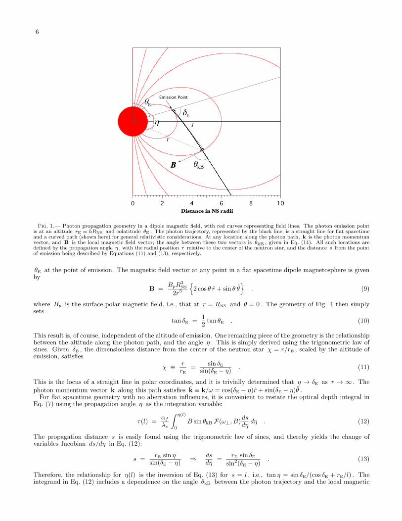
6

1086420

Distance in NS radii

qkB

qE

B

dEh

Emission Point

r

s

Fig. 1.— Photon propagation geometry in a dipole magnetic field, with red curves representing field lines. The photon emission pointis at an altitude rE = hRNS and colatitude θE . The photon trajectory, represented by the black line, is a straight line for flat spacetimeand a curved path (shown here) for general relativistic considerations. At any location along the photon path, k is the photon momentumvector, and B is the local magnetic field vector; the angle between these two vectors is θkB , given in Eq. (14). All such locations aredefined by the propagation angle η , with the radial position r relative to the center of the neutron star, and the distance s from the pointof emission being described by Equations (11) and (13), respectively.

θE at the point of emission. The magnetic field vector at any point in a flat spacetime dipole magnetosphere is givenby

B =BpR

3NS

2r3

2 cos θ r + sin θ θ

. (9)

where Bp is the surface polar magnetic field, i.e., that at r = RNS and θ = 0 . The geometry of Fig. 1 then simplysets

tan δE =12

tan θE . (10)

This result is, of course, independent of the altitude of emission. One remaining piece of the geometry is the relationshipbetween the altitude along the photon path, and the angle η . This is simply derived using the trigonometric law ofsines. Given δE , the dimensionless distance from the center of the neutron star χ = r/rE , scaled by the altitude ofemission, satisfies

χ ≡ rrE

=sin δE

sin(δE − η). (11)

This is the locus of a straight line in polar coordinates, and it is trivially determined that η → δE as r → ∞ . The

photon momentum vector k along this path satisfies k ≡ k/ω = cos(δE − η)r + sin(δE − η)θ .For flat spacetime geometry with no aberration influences, it is convenient to restate the optical depth integral in

Eq. (7) using the propagation angle η as the integration variable:

τ(l) =αfλ–c

∫ η(l)

0

B sin θkB F(ω⊥, B)dsdη

dη . (12)

The propagation distance s is easily found using the trigonometric law of sines, and thereby yields the change ofvariables Jacobian ds/dη in Eq. (12):

s =rE sin η

sin(δE − η)⇒ ds

dη=

rE sin δEsin2(δE − η)

. (13)

Therefore, the relationship for η(l) is the inversion of Eq. (13) for s = l , i.e., tan η = sin δE/(cos δE + rE/l) . Theintegrand in Eq. (12) includes a dependence on the angle θkB between the photon trajectory and the local magnetic

7

field, particularly through the attenuation coefficient function F . The photons start with θkB = 0 , and this angleincreases at first linearly as the photon propagates outward. The angle θkB is given geometrically by

sin θkB =|k×B||k|.|B| =

krBθ − kθBr|B| =

sin θ cos(δE − η)− 2 cos θ sin(δE − η)√1 + 3 cos2 θ

(14)

at every point along the photon’s path. Using Eq. (10) simply demonstrates that the right hand side of this expressionapproaches zero as η = θ−θE → 0 . Note also that by forming cos θkB and using Eq. (11), one can show routinely thatthis result is equivalent to Eq. (5) of Baring & Harding (2007). In the limit of small colatitudes near the magnetic axis,one simply derives sin θkB ≈ 3η/2 , which can be combined with r/rE ≈ 1 + 2η/θE to yield θkB ≈ 3θE(r/rE − 1)/4 .This dependence closely approximates the low altitude values for θkB in flat spacetime exhibited in Fig. 5a of Gonthier& Harding (1994). This completes the general formalism for pair creation optical depth determination in Minkowskimetrics.

3.1. Optical Depth for Emission Near the Magnetic Axis

In order to better understand the character of the optical depth integral, it is instructive to consider the case of aphoton emitted at very small colatitudes. This situation is representative of much of the relevant parameter space foryoung gamma-ray pulsars; for example, the Crab pulsar has a polar cap half-angle of about 4.5 and the Vela pulsarhas a polar cap half-angle of about 2.8 . For these photons emitted very close to the magnetic axis, η and θE aresmall. In this limit, we have the approximations

B ≈ Bp(δE − η)3

h3δ3E

, sin θkB ≈32η (15)

for rE = hRNS . We also have ds/dη ≈ rEδE/(δE − η)2 using Eq. (13), with δE ≈ θE/2 . These results can be insertedinto Eq. (12), and the integration variable changed to x = η/δE , yielding an approximation for the optical depth inaxial locales:

τ(l) ≈ 3θE4

Bph2

αfRNS

λ–

∫ x+

8/(3θEε)

x(1− x)F(

34εθEx,

Bph3 [1− x]

3

)dx , x+ =

ll + hRNS

. (16)

This form is applicable to any choice of the pair conversion function F . Observe that here the the local energy ωhas been replaced with the energy ε seen by an observer at infinity; the two are equivalent in flat spacetime with norotation, but when we consider general relativity and aberration, the distinction will become important. The upperlimit x+ is the value of x = η/δE that realizes a path length l , and is well approximated by l/ (l + hRNS) near themagnetic axis. The lower limit defines the threshold condition, so that if εθE ≤ 8/3 , propagation in flat spacetime outof the magnetosphere never moves the photon above the pair threshold at ω⊥ = 2 , and τ = 0 over the entire photontrajectory. For the particular choice of Erber’s (1966) attenuation coefficient in Eq. (2), the integral for the opticaldepth assumes a fairly simple form:

τErb(l) ≈ 9√

3 θE64√

2

Bph2

αfRNS

λ–

∫ x+

8/(3θEε)

x(1− x) exp

− 32h3

9εBpθE

1x(1− x)3

dx . (17)

If one considers emission points near the magnetic axis at different altitudes along a particular field line with a footpointcolatitude θf , then θE ≈ θf

√h gives the altitude dependence of the emission colatitude. Exploring attenuation opacity

along a fixed field line is germane to treating gamma-ray emission that takes place along or near the last open field line,where θf is fixed by the pulsar’s rotational period. The escape energy εesc can be computed by setting τ(∞) = 1 ,for which x+ → 1 . Imposing this τ(∞) = 1 criterion, and presuming εθE 1 in Eq. (17), yields the approximatealtitude dependence

εesc ∝ h5/2 (18)

for the escape energy. This is a flat spacetime result for near polar axis locales that was identified by Zhang &Harding (2000; see also Lee, et al. 2010). Deviations from this simple altitude dependence arise (i) when the footpointcolatitude θf is not sufficiently small, (ii) if the pair conversion occurs not very far from the ω⊥ = 2 threshold, and(iii) down near the stellar surface where general relativistic effects modify the values of ω , B and θkB .

For significantly sub-critical Bp , a complete asymptotic expression for the optical depth after propagation to highaltitudes can be determined using the method of steepest descents to compute the integral for τ(l) , since the integrandin Eq. (17) is exponentially sensitive to values of x . This is precisely the method employed by Arons & Scharlemann(1979) and later adopted by Hibschman & Arons (2001) in developing similar opacity integrations. The exponentialrealizes a very narrow peak at x = 1/4 , so that for l→∞ and x+ = 1

τErb(l) ≈ 36

219

(3πεB3

pθ3f

2h11/2

)1/2αfRNS

λ–exp

− 213h5/2

35εBpθf

. (19)

This result actually applies for any x+ > 1/4 , i.e. when l & hRNS/3 . It is independent of l since the integrand hassampled beyond the peak and has shrunk to very small values when x exceeds 1/4 by a significant amount. Eq. (19) is

8

in agreement with the approximate optical depth computed by Hibschman & Arons (2001) in their Eq. (8), which wassimilarly formulated to treat gamma-ray propagation above the magnetic pole. Note that Arons & Scharlemann (1979)provided a more general opacity integral by treating magnetic multipole configurations. Again setting τErb(∞) = 1 ,and taking logarithms of Eq. (19), the escape energy εesc for the Erber attenuation coefficient satisfies

εesc =213h5/2

35Bpθf

loge

(36

219αfRNS

λ–

)+

12

loge3πεescB

3pθ

3f

2h11/2

−1

. (20)

While an exact solution for εesc must be determined numerically from this transcendental equation, the secondlogarithmic term on the right is only weakly dependent on its arguments. Therefore, to a good approximation, onecan infer that εesc ∝ 1/Bp and εesc ∝ 1/θf , both of which emerge due to the presence of the factor ω⊥B in theargument of the exponential in Erber’s asymptotic form.

The same protocol can be adopted for pair conversion rates that include threshold modifications, specifically Eq. (3).In this case, as the counterpart of Eq. (16) we have

τ(l) ≈ 3θE4

Bph2

αfRNS

λ–

∫ x+

8/(3θEε)

x(1− x)FBK07

(34εθEx,

Bph3 [1− x]

3

)dx , (21)

again for x+ = l/(l + hRNS) . We can simplify the ensuing analysis by making the substitution λ = 3θEε/8 ≥ 1 sothat locally ω⊥ = 2λx along the trajectory. The argument of the exponential is of the form h3q(x, λ)/Bp where

q(x, λ) ≡ φ(2λx)4(1− x)3 = − 2λx

(1− x)3 −(λx)

2 − 1(1− x)3 loge

(λx− 1λx+ 1

)(22)

Using the method of steepest descents once again, we take the first derivative of the function in the exponential, andset it equal to zero to find the peak of the function. The solution of ∂q/∂x = 0 is a transcendental function in λ , butit can be numerically approximated to better than 3% by

x ≈ 1

4+ 0.82λ−5/3. (23)

Given ∂q/∂x = 0, the logarithmic term loge[(λx − 1)/(λx + 1)] can be expressed algebraically, and q′′(x, λ) can bewritten in the following form:

q′′(x, λ) =8λ[λ2(2x3 − 3x+ 1

)− 3x+ 3

](λ2x(x+ 2)− 3)(1− x)5(λ2x2 − 1)

. (24)

The integral is then given approximately, as before, by the method of steepest descents. With some cancellation, wethen obtain

τBK07 ≈αfRNS

λ–

[3(λx)2 − 1] (λx− 1)

2ε λ2x (λx+ 1)

[πχ3B3

p

2(x+ 2) (1− x) |Υ|h7

]1/2

exp

− h3

Bpχ

(25)

where

Υ =(1− 2x− 2x2

)+

3λ2 , χ =

(1− x)2

4λ

λ2x(x+ 2)− 3

. (26)

Here Υ is employed to render the q′′(x, λ) term more compact, and χ = 1/q(x, λ) . Noting that θf ≈ 8λ/(3ε√h) in

this small colatitude limit, Eq. (25) agrees with the Erber approximation in Eq. (19) to high precision in the regimewhere λ → ∞ , and exhibits the appropriate threshold behavior. Setting τ(∞) = 1 gives a transcendental equationthat can be solved numerically for εesc . The impressive precision of this analytic steepest descents result for the escapeenergy is apparent in Fig. 3 below.

Well above the escape energy, the pair attenuation length l is far inferior to the neutron star radius. For surfaceemission (h = 1 ), in this l RNS limit, we can assert x+ 1 in Eq. (16), so that series expansion in the xintegration variable yields

τ(l) ≈ 3θE4

αfRNS

λ–Bp

∫ x+

8/(3θEε)

xF(

34εθEx, Bp [1− 3x]

)dx , x+ 1 . (27)

Analytic reduction of this integral is fairly complicated for the case of the FB88 rate, but is relatively amenable for theErber form, which we employ at this juncture. Inserting Eq. (2) for F , because of the strong exponential dependenceof the integrand, the dominant contribution to the integral comes from x ≈ x+ . Replacing the factor of x in theintegrand that lies outside the exponential by x3

+/x2 , for x+ ≈ l/RNS , yields

τ(l) ≈ 9√

3BpθE64√

2

αfRNS

λ–

(l

RNS

)3

exp

32

3εBpθE

∫ x+

8/(3θEε)

exp

− 32

9εBpθE

1x

dxx2 . (28)

9

This manipulation affords analytic evaluation of the integral. The attenuation length L is obtained by setting τ(L) = 1in the resulting equation for τ(l) , which after rearrangement leads to

exp

− 32RNS

9εBpθEL

≈ 2048

√2

81√

3 εB2pθ

2E

λ–αfRNS

(RNS

L

)3

exp

− 32

3εBpθE

+ exp

− 4

3Bp

. (29)

In general, solutions for L are realized when the second exponential term on the right hand side of Eq. (29) can beneglected, at the < 10−3 level. This simplifies the algebra, and taking logarithms, one arrives at

RNS

L≈ 3 +

9εBpθE32

loge

[81√

3 εB2pθ

2E

2048√

2

αfL3

λ–R2NS

]. (30)

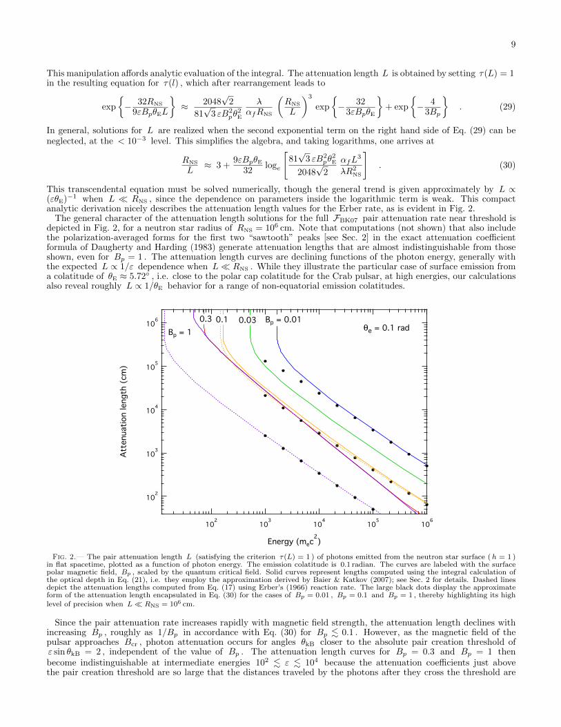
This transcendental equation must be solved numerically, though the general trend is given approximately by L ∝(εθE)−1 when L RNS , since the dependence on parameters inside the logarithmic term is weak. This compactanalytic derivation nicely describes the attenuation length values for the Erber rate, as is evident in Fig. 2.

The general character of the attenuation length solutions for the full FBK07 pair attenuation rate near threshold isdepicted in Fig. 2, for a neutron star radius of RNS = 106 cm. Note that computations (not shown) that also includethe polarization-averaged forms for the first two “sawtooth” peaks [see Sec. 2] in the exact attenuation coefficientformula of Daugherty and Harding (1983) generate attenuation lengths that are almost indistinguishable from thoseshown, even for Bp = 1 . The attenuation length curves are declining functions of the photon energy, generally withthe expected L ∝ 1/ε dependence when L RNS . While they illustrate the particular case of surface emission froma colatitude of θE ≈ 5.72 , i.e. close to the polar cap colatitude for the Crab pulsar, at high energies, our calculationsalso reveal roughly L ∝ 1/θE behavior for a range of non-equatorial emission colatitudes.

102

103

104

105

106

Att

enuati

on length

(cm

)

102

103

104

105

106

Energy (mec2)

Bp = 0.010.030.10.3

Bp = 1θe = 0.1 rad

Fig. 2.— The pair attenuation length L (satisfying the criterion τ(L) = 1 ) of photons emitted from the neutron star surface (h = 1 )in flat spacetime, plotted as a function of photon energy. The emission colatitude is 0.1 radian. The curves are labeled with the surfacepolar magnetic field, Bp , scaled by the quantum critical field. Solid curves represent lengths computed using the integral calculation ofthe optical depth in Eq. (21), i.e. they employ the approximation derived by Baier & Katkov (2007); see Sec. 2 for details. Dashed linesdepict the attenuation lengths computed from Eq. (17) using Erber’s (1966) reaction rate. The large black dots display the approximateform of the attenuation length encapsulated in Eq. (30) for the cases of Bp = 0.01 , Bp = 0.1 and Bp = 1 , thereby highlighting its highlevel of precision when L RNS = 106 cm.

Since the pair attenuation rate increases rapidly with magnetic field strength, the attenuation length declines withincreasing Bp , roughly as 1/Bp in accordance with Eq. (30) for Bp . 0.1 . However, as the magnetic field of thepulsar approaches Bcr , photon attenuation occurs for angles θkB closer to the absolute pair creation threshold ofε sin θkB = 2 , independent of the value of Bp . The attenuation length curves for Bp = 0.3 and Bp = 1 thenbecome indistinguishable at intermediate energies 102 . ε . 104 because the attenuation coefficients just abovethe pair creation threshold are so large that the distances traveled by the photons after they cross the threshold are

10

minuscule in comparison with the propagation distance required to reach the threshold. At the very highest energies,the Bp = 0.3 and Bp = 1 curves begin to diverge again because the attenuation coefficients drop by several ordersof magnitude and the distance a Bp = 0.3 photon travels after crossing the threshold before converting becomescomparable to the distance it transits before reaching the point where ε sin θkB = 2 .

The dashed curves display the attenuation lengths for Erber rate formalism [see Eq. (17)]. Since the Erber formsignificantly overestimates the attenuation coefficient near pair threshold, it generates shorter attenuation lengths thandoes the more precise determination using Eq. (21). The analytic approximation in Eq. (30) to the Erber τ(L) = 1formalism is also shown as discrete dots, demonstrating a good precision in matching the fully numerical curves at highenergies. This approximation provides a useful guide to the generic character of attenuation in L RNS domains. Thevertical upturns in the curves at low energies define the photon escape energies εesc for each Bp case; such featuresare the focus of Section 3.2, and demarcate the energy domains for pair creation transparency of the magnetosphere.

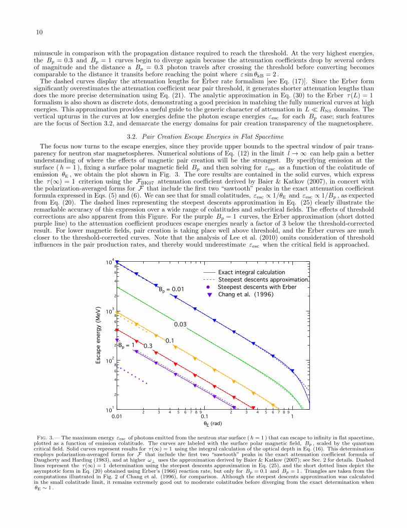
3.2. Pair Creation Escape Energies in Flat Spacetime

The focus now turns to the escape energies, since they provide upper bounds to the spectral window of pair trans-parency for neutron star magnetospheres. Numerical solutions of Eq. (12) in the limit l →∞ can help gain a betterunderstanding of where the effects of magnetic pair creation will be the strongest. By specifying emission at thesurface (h = 1 ), fixing a surface polar magnetic field Bp and then solving for εesc as a function of the colatitude ofemission θE , we obtain the plot shown in Fig. 3. The core results are contained in the solid curves, which expressthe τ(∞) = 1 criterion using the FBK07 attenuation coefficient derived by Baier & Katkov (2007), in concert withthe polarization-averaged forms for F that include the first two “sawtooth” peaks in the exact attenuation coefficientformula expressed in Eqs. (5) and (6). We can see that for small colatitudes, εesc ∝ 1/θE and εesc ∝ 1/Bp , as expectedfrom Eq. (20). The dashed lines representing the steepest descents approximation in Eq. (25) clearly illustrate theremarkable accuracy of this expression over a wide range of colatitudes and subcritical fields. The effects of thresholdcorrections are also apparent from this Figure. For the purple Bp = 1 curves, the Erber approximation (short dottedpurple line) to the attenuation coefficient produces escape energies nearly a factor of 3 below the threshold-correctedresult. For lower magnetic fields, pair creation is taking place well above threshold, and the Erber curves are muchcloser to the threshold-corrected curves. Note that the analysis of Lee et al. (2010) omits consideration of thresholdinfluences in the pair production rates, and thereby would underestimate εesc when the critical field is approached.

101

2

4

6

810

2

2

4

6

810

3

2

4

6

810

4

Esc

ape e

nerg

y (

MeV

)

0.012 3 4 5 6 7 8 9

0.12 3 4 5 6 7 8 9

1

θE (rad)

Exact integral calculation

Steepest descents approximation

Steepest descents with Erber

Chang et al. (1996)

Bp = 1 0.30.1

0.03

Bp = 0.01

Fig. 3.— The maximum energy εesc of photons emitted from the neutron star surface (h = 1 ) that can escape to infinity in flat spacetime,plotted as a function of emission colatitude. The curves are labeled with the surface polar magnetic field, Bp , scaled by the quantumcritical field. Solid curves represent results for τ(∞) = 1 using the integral calculation of the optical depth in Eq. (16). This determinationemploys polarization-averaged forms for F that include the first two “sawtooth” peaks in the exact attenuation coefficient formula ofDaugherty and Harding (1983), and at higher ω⊥ uses the approximation derived by Baier & Katkov (2007); see Sec. 2 for details. Dashedlines represent the τ(∞) = 1 determination using the steepest descents approximation in Eq. (25), and the short dotted lines depict theasymptotic form in Eq. (20) obtained using Erber’s (1966) reaction rate, but only for Bp = 0.1 and Bp = 1 . Triangles are taken from thecomputations illustrated in Fig. 2 of Chang et al. (1996), for comparison. Although the steepest descents approximation was calculatedin the small colatitude limit, it remains extremely good out to moderate colatitudes before diverging from the exact determination whenθE ∼ 1 .

11

In comparing with extant flat spacetime computations of escape energies, our results realize good agreement withFig. 2 of Ho, Epstein & Fenimore (1990), using the Erber asymptotic form of Eq. (2); this matches their chosenattenuation coefficient closely. In this analysis, we assume that photons are always emitted parallel to the magneticfield, so comparison of our results is made to the topmost (ψi = 0 ) curve of their Fig. 2, the x-axis of which isequivalent to log(δE + θE) in our variables. For B = 2 × 1012 Gauss, the apparent difference between our numericsand theirs is less than about 15% , though visual precision in reading this plot limits such an estimate. For the Erberattenuation coefficient in flat spacetime, multiplying the photon escape energy from a fixed emission altitude andcolatitude by the surface polar magnetic field yields an approximately constant result.

If, on the other hand, one fixes the surface polar field and the photon energy, and calculates the lowest altitudermin from which photons of that energy can escape to infinity, one can formulate a “pair convertosphere” plot likethat in Fig. 4, which is computed for flat spacetime. The leaf-shaped curves represent a cross-section through a τ = 1surface that is symmetric about the magnetic axis. Inside the surface, to a first approximation, all photons of thelabeled energy will convert to pairs. Outside the surface, photons can escape and be detected. At a fixed colatitude,a higher altitude of emission results in a higher escape energy (corresponding to shifting the curves in Fig. 3 up inenergy). In a Minkowski metric, all of these minimum altitude curves drop to below the stellar surface at the magneticpole, since there the field line radius of curvature is very large, and photons do not quickly encounter significant θkB

during propagation when initially emitted parallel to the local field. Rotational aberration influences, which will beconsidered in Section. 5 below, introduce an azimuthal asymmetry about the magnetic axis for an inclined pulsar,and significantly distort the shape of the surfaces near the magnetic poles, but not by much in equatorial regions.General relativistic influences (discussed in Section 4) are significant below 2RNS , and while they do not appreciablyalter the overall morphology of the leaf-shaped contours, they do force them to high slightly altitudes above the poles.Rotational aberration distorts the morphology of these τ = 1 curves somewhat, introducing asymmetry between theleading and trailing edges, along the lines of the magnetospheric cross section plot in Fig. 3 of Harding, Tademaru &Esposito (1978).

-10

-5

0

5

10

-10 -5 0 5 10

500 MeV

1 GeV

2 GeV

5 GeV

10 GeV

Bp = 3.79 x 1012

G

Fig. 4.— “Pair convertosphere” diagram for a pulsar with the same magnetic field as the Crab, for flat spacetime and the specific case ofno rotational/aberration influences. Dipolar field structure (depicted in light red) underlays each leaf-shaped green curve, which representsthe lowest possible emission point at a given colatitude for a photon of a fixed energy (as labelled), below which magnetic pair creationwould attenuate the photon before it could escape from the neutron star magnetosphere. The photons are always presumed to be emittedparallel to the local field. The scale is neutron star radii, with the unit radius circle in the center representing the neutron star. Generalrelativistic effects alter these curves only very near the neutron star surface, and then only modestly, moving them to slightly higheraltitudes.

12

As the pair convertosphere minimum altitude contours move to equatorial regions, it is clear that rmin is a mono-tonically increasing function of colatitude θE . Photons emitted above the equator more readily transit across the fieldlines than in polar locales, and so have shorter attenuation lengths. This is because the magnetic field lines possessshorter radii of curvature in equatorial zones than in polar regions, at a given emission altitude. Hence, for a fixedphoton energy, in order to compensate and increase L to infinity, the local field strengths sampled must be lowered,forcing the required θkB at the instant of conversion to larger values. Thus, the minimum altitudes must rise as θEdoes, and the result is the leaf-shaped morphology in Fig. 3. For moderately small colatitudes, this trend can bediscerned from Eq. (20), namely the Erber asymptotic form for the escape energy. It is noteworthy that this behaviorcontradicts that displayed in Figure 3 of Lee et al. (2010), where their rmin values drop for colatitudes θ & 60 , adecline that does not appear to depend on aberrational influences in their work. It is not clear why this behavior iselicited in their computations. In Section 5, we demonstrate that rotational/aberrational influences on escape energyand minimum altitude determinations at these equatorial colatitudes are comparatively small.

4. GENERAL RELATIVISTIC EFFECTS

Our overall approach to calculating curved spacetime effects on photon attenuation will be to integrate the opticaldepth over path length intervals in the local inertial frame (hereafter LIF), with all magnetic fields, angles, energies,and distances computed in that frame. In general, we will use the definitions for curved spacetime quantities fromGonthier & Harding (1994, hereafter GH94), with the notation altered slightly for clarity. Our starting point is againEq. (7), therefore requiring specification of the quantities B , ω and θkB in the LIF. The blueshift of the photonenergy in the LIF from its value ε ≡ ω∞ at infinity (i.e. as observed) can be accounted for with the simple correction

ω =ε√

1−Ψ, Ψ =

rsr≡ 2GM

c2r(31)

at radius r , where rs = 2GM/c2 is the Schwarzschild radius of a neutron star of mass M . The introduction ofthe dimensionless parameter Ψ to describe the radial position will expedite the path length integration in curvedspacetime constructs; we will use it as our integration variable instead of η in Eq. (12), approximately equivalentlyto the approach of GH94. The emission altitude rE will be prescribed by ΨE = rs/rE < 1 . Note that throughout, wewill adopt the convention that ε shall denote the dimensionless photon energy as seen by an observer, and ω shallsignify that in the LIF.

The general relativistic form of a dipole magnetic field in a Schwarzschild metric was developed in Wasserman &Shapiro (1983). It is also expressed in Eq. (21) of GH94 in the LIF in terms of the coordinates r and θ for an observerat infinity:

BGR =− 3Bp cos θ

r2sr

[rrs

loge

(1− rs

r

)+ 1 +

rs2r

]r

(32)

+ 3Bp sin θ

r2sr

[(rrs− 1

)loge

(1− rs

r

)+ 1− rs

2r

]θ√

1− rs/r.

In flat spacetime, where rs r , Bp represents the surface polar field at θ = 0 . It is more convenient to write thisin terms of the scaled inverse radius Ψ = rs/r . To this end we define the functions

ξr(x) =− 1

x3

[loge(1− x) + x+

x2

2

](33)

ξθ(x) =1

x3√

1− x

[(1− x) loge(1− x) + x− x2

2

].

Then, the curved spacetime dipole field is expressed via

BGR = 3BpΨ

3

r3s

ξr(Ψ) cos θ r + ξθ(Ψ) sin θ θ

. (34)

In flat spacetime, where Ψ 1 , the leading terms of the Taylor series expansion yield ξr(Ψ) ≈ 1/3 and ξθ(Ψ) ≈ 1/6 ,so that then Eq. (34) reproduces the familar result in Eq. (9) in the absence of general relativity. The magnitude ofthe general relativistic field is then

BGR = 3BpΨ

3

r3s

√[ξr(Ψ)]2 cos2 θ + [ξθ(Ψ)]2 sin2 θ ; (35)

this will be employed in the quantum pair creation rates in the local inertial frame. The ratio of Eq. (35) for altitudesnear the surface to its flat spacetime value (i.e., Ψ→ 0 ) inferred from Eq. (9) reproduces the ratio plotted in Fig. 5cof GH94.

The trajectory of a photon emitted from a point in a neutron star magnetosphere will be curved in the frame ofan observer at infinity, though for cases of emission near the polar cap, this is generally small (see Baring & Harding

13

2001). Here we incorporate the influence of the slight curvature in the path, so that calculating sin θkB becomesa slightly more complicated exercise than it was in the flat spacetime approximation. First, the photon is emittedparallel to the magnetic field in the LIF. This fixes δE , the initial angle between the photon trajectory and the radialdirection (depicted in Fig. 1):

sin δE ≡Bθ

B

∣∣∣∣r=Re

=sin θE ξθ(ΨE)√

cos2 θE [ξr(ΨE)]2

+ sin2 θE [ξθ(ΨE)]2

. (36)

When ΨE 1 , this reduces to Eq. (10), though in general, since ξθ(ΨE)/ξr(ΨE) ≈ 1/2 + ΨE/8 +O(Ψ2E) in this limit,

it is easily seen that spacetime curvature increases δE for proximity to the magnetic pole. This effect is illustrated inFigure 3b of GH94. The photon’s trajectory at infinity emerges parallel to a line drawn from the center of the star,displaced from it by a distance b . This impact parameter b is proportional to the ratio of two conserved quantities ofthe unbound photon orbit, the orbital angular momentum and the energy; consult Pechenick, Ftaclas & Cohen (1983)or Chapter 8 of Weinberg (1972) for illustrations of such orbits. Scaling b by the Schwarzschild radius, as we havewith r , introduces a new trajectory parameter Ψb = rs/b that can be related to ΨE and δE via

Ψb =ΨE

sin δE

√1−ΨE ≡ ΨE

√(1−ΨE)

1 + [ξ(ΨE)]

2cot2 θE

, (37)

where

ξ(Ψ) =ξr(Ψ)ξθ(Ψ)

. (38)

The first identity in Eq. (37) is derived from Eq. (17) of GH94 (correcting a typographical error therein: see Eq. (A2) ofHBG97), who use the notation δ0 for δE . Observe that the impact parameter can be smaller than the Schwarzschildradius for almost radial trajectories initiated near the magnetic polar axis (setting sin δE 1 ), so Ψb can assumevalues well in excess of unity where the orbit is a capture one, if reversed. Inserting Eq. (36) to substitute for sin δEthen yields Ψb purely as a function of the emission altitude (i.e. ΨE ) and colatitude θE , and derives the secondidentity in Eq. (37), with 0 ≤ ξ(Ψ) ≤ 2 on the interval 0 ≤ Ψ ≤ 1 .

This second form for Ψb is needed for the photon trajectory computation, an integral expression for which is givenin Eq. (11) of GH94:

θ(Ψ) ≡ θE + ∆θ = θE +

∫ ΨE

Ψ

dΨr√Ψ2b −Ψ2

r(1−Ψr), (39)

expressing the functional dependence θ(r) , as viewed by an observer at infinity. An alternative version of this canbe obtained from Eq. (8.5.6) of Weinberg (1972); see also Misner, Thorne & Wheeler (1973). Since Ψ ≤ ΨE in thisconstruction, as the photon propagates out from the star, then the change in colatitude ∆θ is necessarily positiveas the altitude r increases. Observe that Ψ2

b > Ψ2E(1 − ΨE) from the second identity in Eq. (37) so that the

argument of the square root in the integrand of Eq. (39) is positive-definite. In the case of a neutron star, generallyΨE . 0.4 , and the integral in Eq. (39) can be approximated extremely accurately by an analytic form, for non-equatorial emission colatitudes θE . π/4 ; see the Appendix for details. This expedient step removes the trajectoryintegral from consideration, and speeds up optical depth computations immensely. In the flat spacetime limit, ΨE 1 ,the integral for the trajectory in Eq. (39) can be expressed analytically by replacing the argument of the square rootin the denominator by Ψ2

b − Ψ2r . Then, forming sin ∆θ , the result can be inverted to solve for Ψ and thereby find

the locus for the trajectory:

Ψ = Ψb sin

(θE − θ − arcsin

ΨE

Ψb

). (40)

This is a polar coordinate form for a straight line, and is easily shown to be equivalent to Eq. (11) using the limiting

form Ψb ≈ ΨE

√1 + 4 cot2 θE ≈ ΨE/ sin δE when ΨE 1 .

Given emission locale coordinates ( ΨE, θE ), for any subsequent position ( Ψ, θ ) along the curved trajectory, we candetermine the angle θkB of the photon momentum to the local field direction, in the LIF. This is simply done byforming a cross product between the photon momentum kGR and BGR using Eq. (34) for the field. The photonmomentum in the LIF can be derived from the formalism in Section 3 of GH94, or by manipulation of the differentialform of the trajectory equation in Eq. (39), i.e. setting kθ/kr = dθ/dr = −(Ψ/r) dθ/dΨ and then normalizing toEq. (31). The result is

kGR =ε

Ψb

√1−Ψ

√Ψ2b −Ψ2(1−Ψ) r + Ψ

√1−Ψ θ

, (41)

which can be simply inferred from Eq. (A1) of Harding, Baring & Gonthier (1997). ¿From this, one can form theangle δE for the initial angle of the photon momentum relative to the radial direction, via sin δE = |kGR× r|/|kGR| =ΨE

√1−ΨE /Ψb , a result that is the first identity in Eq. (37). Forming a cross product between the photon momentum

14

and the field vectors, it follows that

sin θkB ≡|kGR ×BGR||kGR|.|BGR|

=Bθ

B

[1− (1−Ψ)

Ψ2

Ψ2b

]1/2

− Br

BΨ(1−Ψ)1/2

Ψb, (42)

an expression that is also routinely obtained by rearranging Eq. (37) of GH94. Inserting the forms for the fieldcomponents, elementary manipulations yield

sin θkB =

√Ψ2b −Ψ2(1−Ψ)−Ψ

√1−Ψ ξ(Ψ) cot θ

Ψb

√1 + [ξ(Ψ)]

2cot2 θ

(43)

Employing the second form for Ψb in Eq. (37) quickly reveals that when Ψ = ΨE , this expression yields sin θkB = 0 .Using the fact that Ψ2(1−Ψ) is an increasing function for 0 < Ψ < 2/3 , and that ξ(Ψ) is a more modestly decliningfunction of Ψ on the same interval, it is routinely established that sin θkB increases as r increases from the emissionradius, i.e. Ψ drops below ΨE . Numerical comparisons of our computations of sin θkB and the effective pair threshold2/ sin θkB with panels (a) and (b) of Fig. 5 of GH94 were performed, yielding excellent agreement. In the flat spacetimelimit ΨE 1 , Ψb ≈ ΨE/ sin δE ≈ Ψ/ sin(δE − η) can be deduced using Eq. (11), and then it is straightforward todemonstrate that Eq. (43) reduces to Eq. (14).

Finally, we choose to change our integration variable from s to Ψ . In the LIF, the path length is related to thecoordinate transit time: ds2 = (1−Ψ)c2dt2 in the Schwarzschild case. Equivalently, the path length can be connectedto the radial and angular (equatorial) contributions to the Schwarzschild metric via ds2 = dr2/(1−Ψ) + r2 dθ2 . Thetwo forms are equivalent, yielding the proper time interval dτ2 = 0 for light-like propagation. Employing Eq. (18)of GH94, or equivalently taking the derivative of Eq. (8.7.2) of Weinberg (1972), yields an expression for dt/dΨ forthe photon’s transit along its trajectory, essentially formulae for Shapiro delay. Assembling these pieces one quicklyarrives at the change of variables

dsrE

= − ΨE Ψb dΨ

Ψ2√

(1−Ψ) Ψ2b −Ψ2(1−Ψ)

. (44)

The optical depth integration for the case of including general relativity then takes the form

τ(Ψ) = rE ΨE

∫ ΨE

Ψ

R(ω, sin θkB, BGR) Ψb dΨr

Ψ2r

√(1−Ψr) Ψ2

b −Ψ2r(1−Ψr)

, (45)

where the arguments of the scaled quantum pair creation rate R are given by Eqs. (31), (35) and (43). With thisconstruct, we can formally define the attenuation length L as in Harding, Baring & Gonthier (1997) and Baring &Harding (2001) via

τ (ΨL) = 1 ; s (ΨL) = L . (46)

L is approximately the cumulative LIF distance that a photon of a given energy will travel from its emission pointbefore converting to an electron-positron pair. When ΨE 1 , Eq. (45) is equivalent to the flat spacetime evaluationin Eq. (12).

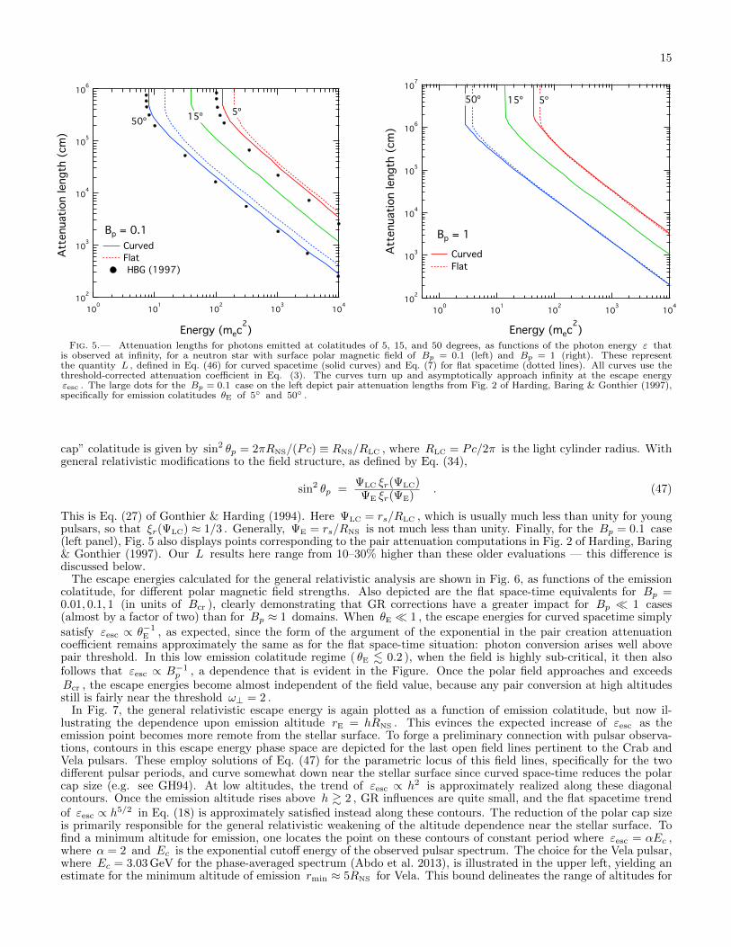
Figure 5 displays the attenuation lengths computed for curved spacetime at two different magnetic fields. These areevaluated specifically for emission from the neutron star surface. The curves are monotonically declining functions ofphoton energy ε as observed at infinity. At high energies, where L RNS , pair attenuation occurs very close to thesurface and general relativistic effects modify the field structure and photon trajectory and redshift in a manner thatis essentially independent of ε . Accordingly, for the B = 0.1 example, a dependence L ∝ (εθE)−1 is approximatelyrealized, just like the Minkowski spacetime dependence deduced from Eq. (30), but with a smaller coefficient ofproportionality in the GR case. The influence of curved spacetime reduces L slightly, primarily because it amplifiesboth the field strength and the photon energy in the LIF. In the B = 1 example, the GR-corrected and flat spacetimeattenuation lengths are almost identical because photon conversion arises very soon after pair threshold (ω⊥ = 2) inthe LIF is crossed during propagation. The trajectories then sample regimes ΨE Ψb before attenuation, so thatthe path length differential in Eq. (44) approximately satisfies ds/dr ≈ 1/

√1−ΨE , using dr/r = −dΨ/Ψ . Hence

the post-Newtonian GR correction to the path length s = L is precisely that for the blueshift of the photon energy inthe LIF. Accordingly, the computation of L in such threshold-conversion domains is insensitive to general relativisticmodifications.

At low energies, the curves turn up and asymptotically approach infinity at the escape energy εesc . A small shiftin escape energy is evident, due largely to the gravitational redshifting of the photon energy. The monotonic trend ofdecreasing L and εesc with increasing colatitude θE of emission is a result of increased field line curvature away fromthe magnetic polar regions. The footpoint emission colatitude θf ≡ θE can be coupled to a pulsar rotation period ifit is assumed to be applicable to the last open field line, θf → θp . For a dipolar field in flat space-time this “polar

15

102

103

104

105

106

Att

enuati

on length

(cm

)

100

101

102

103

104

Energy (mec2)

5¼50¼

Bp = 0.1

Curved

Flat

HBG (1997)

15¼

102

103

104

105

106

107

Att

enuati

on length

(cm

)

100

101

102

103

104

Energy (mec2)

5¼15¼50¼

Bp = 1

Curved

Flat

Fig. 5.— Attenuation lengths for photons emitted at colatitudes of 5, 15, and 50 degrees, as functions of the photon energy ε thatis observed at infinity, for a neutron star with surface polar magnetic field of Bp = 0.1 (left) and Bp = 1 (right). These representthe quantity L , defined in Eq. (46) for curved spacetime (solid curves) and Eq. (7) for flat spacetime (dotted lines). All curves use thethreshold-corrected attenuation coefficient in Eq. (3). The curves turn up and asymptotically approach infinity at the escape energyεesc . The large dots for the Bp = 0.1 case on the left depict pair attenuation lengths from Fig. 2 of Harding, Baring & Gonthier (1997),specifically for emission colatitudes θE of 5 and 50 .

cap” colatitude is given by sin2 θp = 2πRNS/(Pc) ≡ RNS/RLC , where RLC = Pc/2π is the light cylinder radius. Withgeneral relativistic modifications to the field structure, as defined by Eq. (34),

sin2 θp =ΨLC ξr(ΨLC)ΨE ξr(ΨE)

. (47)

This is Eq. (27) of Gonthier & Harding (1994). Here ΨLC = rs/RLC , which is usually much less than unity for youngpulsars, so that ξr(ΨLC) ≈ 1/3 . Generally, ΨE = rs/RNS is not much less than unity. Finally, for the Bp = 0.1 case(left panel), Fig. 5 also displays points corresponding to the pair attenuation computations in Fig. 2 of Harding, Baring& Gonthier (1997). Our L results here range from 10–30% higher than these older evaluations — this difference isdiscussed below.

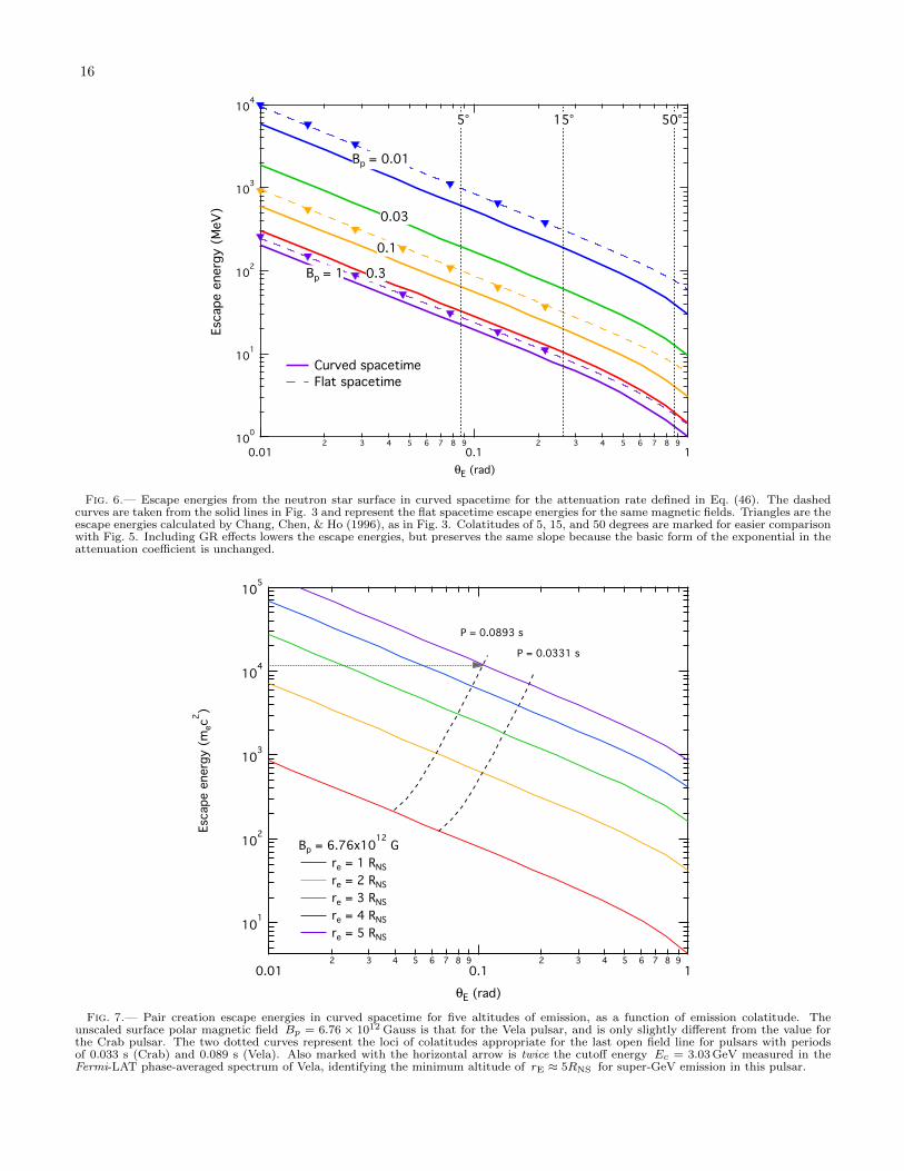
The escape energies calculated for the general relativistic analysis are shown in Fig. 6, as functions of the emissioncolatitude, for different polar magnetic field strengths. Also depicted are the flat space-time equivalents for Bp =0.01, 0.1, 1 (in units of Bcr ), clearly demonstrating that GR corrections have a greater impact for Bp 1 cases(almost by a factor of two) than for Bp ≈ 1 domains. When θE 1 , the escape energies for curved spacetime simply

satisfy εesc ∝ θ−1E , as expected, since the form of the argument of the exponential in the pair creation attenuation

coefficient remains approximately the same as for the flat space-time situation: photon conversion arises well abovepair threshold. In this low emission colatitude regime ( θE . 0.2 ), when the field is highly sub-critical, it then alsofollows that εesc ∝ B−1

p , a dependence that is evident in the Figure. Once the polar field approaches and exceedsBcr , the escape energies become almost independent of the field value, because any pair conversion at high altitudesstill is fairly near the threshold ω⊥ = 2 .

In Fig. 7, the general relativistic escape energy is again plotted as a function of emission colatitude, but now il-lustrating the dependence upon emission altitude rE = hRNS . This evinces the expected increase of εesc as theemission point becomes more remote from the stellar surface. To forge a preliminary connection with pulsar observa-tions, contours in this escape energy phase space are depicted for the last open field lines pertinent to the Crab andVela pulsars. These employ solutions of Eq. (47) for the parametric locus of this field lines, specifically for the twodifferent pulsar periods, and curve somewhat down near the stellar surface since curved space-time reduces the polarcap size (e.g. see GH94). At low altitudes, the trend of εesc ∝ h2 is approximately realized along these diagonalcontours. Once the emission altitude rises above h & 2 , GR influences are quite small, and the flat spacetime trendof εesc ∝ h5/2 in Eq. (18) is approximately satisfied instead along these contours. The reduction of the polar cap sizeis primarily responsible for the general relativistic weakening of the altitude dependence near the stellar surface. Tofind a minimum altitude for emission, one locates the point on these contours of constant period where εesc = αEc ,where α = 2 and Ec is the exponential cutoff energy of the observed pulsar spectrum. The choice for the Vela pulsar,where Ec = 3.03 GeV for the phase-averaged spectrum (Abdo et al. 2013), is illustrated in the upper left, yielding anestimate for the minimum altitude of emission rmin ≈ 5RNS for Vela. This bound delineates the range of altitudes for

16

100

101

102

103

104

Esc

ape e

nerg

y (

MeV

)

0.012 3 4 5 6 7 8 9

0.12 3 4 5 6 7 8 9

1

θE (rad)

Bp = 0.01

Bp = 1 0.3

0.1

0.03

Curved spacetime

Flat spacetime

5¡ 15¡ 50¡

Fig. 6.— Escape energies from the neutron star surface in curved spacetime for the attenuation rate defined in Eq. (46). The dashedcurves are taken from the solid lines in Fig. 3 and represent the flat spacetime escape energies for the same magnetic fields. Triangles are theescape energies calculated by Chang, Chen, & Ho (1996), as in Fig. 3. Colatitudes of 5, 15, and 50 degrees are marked for easier comparisonwith Fig. 5. Including GR effects lowers the escape energies, but preserves the same slope because the basic form of the exponential in theattenuation coefficient is unchanged.

101

102

103

104

105

Esc

ape e

nerg

y (

mec

2)

0.012 3 4 5 6 7 8 9

0.12 3 4 5 6 7 8 9

1

θE (rad)

Bp = 6.76x1012

G

re = 1 RNS

re = 2 RNS

re = 3 RNS

re = 4 RNS

re = 5 RNS

P = 0.0893 s

P = 0.0331 s

Fig. 7.— Pair creation escape energies in curved spacetime for five altitudes of emission, as a function of emission colatitude. Theunscaled surface polar magnetic field Bp = 6.76 × 1012 Gauss is that for the Vela pulsar, and is only slightly different from the value forthe Crab pulsar. The two dotted curves represent the loci of colatitudes appropriate for the last open field line for pulsars with periodsof 0.033 s (Crab) and 0.089 s (Vela). Also marked with the horizontal arrow is twice the cutoff energy Ec = 3.03 GeV measured in theFermi-LAT phase-averaged spectrum of Vela, identifying the minimum altitude of rE ≈ 5RNS for super-GeV emission in this pulsar.

17

which pair transparency is achieved in the magnetosphere of a given pulsar, for emission along the last open field line.This protocol for constraining the emission zones of pulsars is discussed at greater length in Section. 6.

The pair production attenuation lengths and escape energies computed here differ slightly from those presented inHarding, Baring & Gonthier (1997) and Baring & Harding (2001). The attenuation lengths in Fig. 5 are systematicallyhigher by around 10% than those in the left panel of Fig. 2 of Harding, Baring & Gonthier (1997). The escape energiesin Fig. 6 are higher than the corresponding evaluations in Harding, Baring & Gonthier (1997) by around 20-30%. Theorigin of this difference is presently unclear. We observe that there appears to be a slight disagreement between thevalues of sin θkB computed in Harding, Baring & Gonthier (1997) for curved spacetime and those derived in this workand in Gonthier & Harding (1994), with those in Harding, Baring & Gonthier (1997) being about 15–20% higher. Thisis consistent with the slightly lower values of L and εesc computed in Harding, Baring & Gonthier (1997) relative tothose here. As noted above, there is excellent agreement between our geometry and attenuation coefficient calculationsand those presented in Gonthier & Harding (1994). Our numerical results for the GR case map continuously over tothe ΨE → 0 flat spacetime cases illustrated in Sec. 3. These latter checks indicate that the curved spacetime resultspresented here appear to be robust.

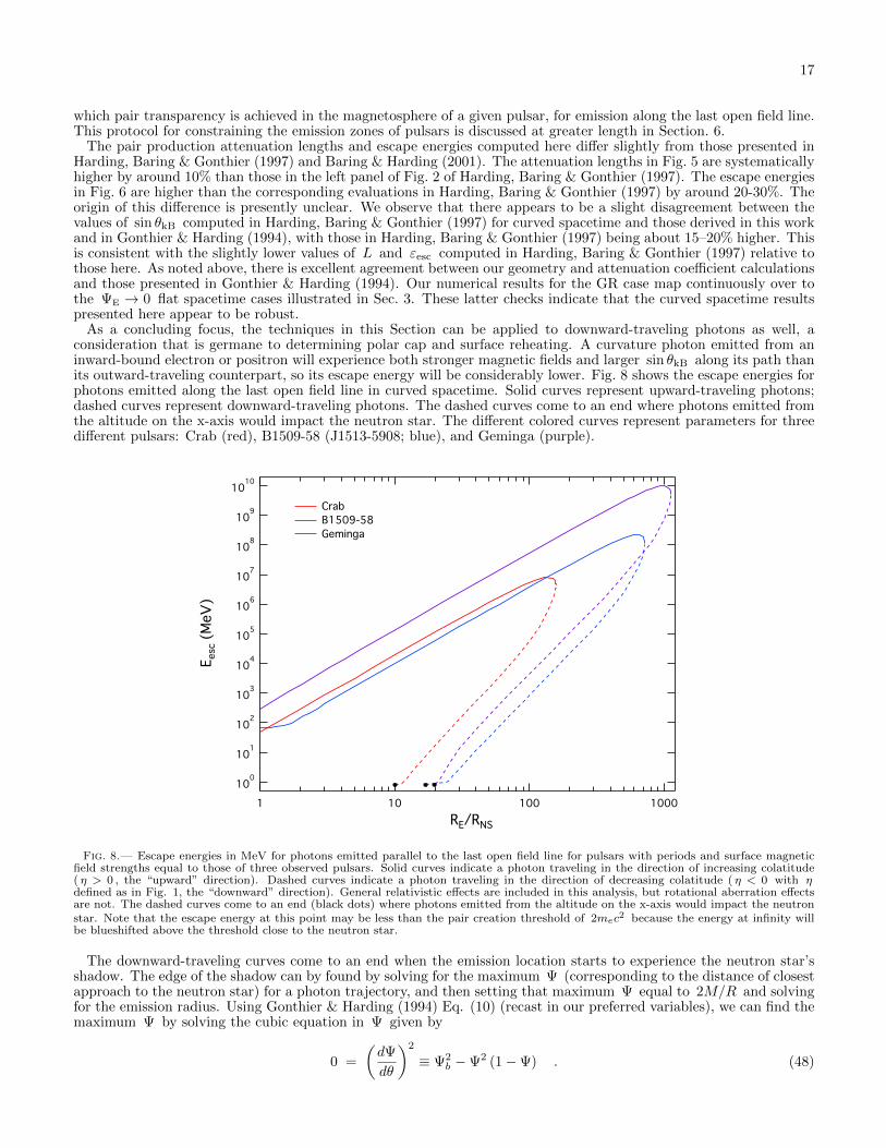
As a concluding focus, the techniques in this Section can be applied to downward-traveling photons as well, aconsideration that is germane to determining polar cap and surface reheating. A curvature photon emitted from aninward-bound electron or positron will experience both stronger magnetic fields and larger sin θkB along its path thanits outward-traveling counterpart, so its escape energy will be considerably lower. Fig. 8 shows the escape energies forphotons emitted along the last open field line in curved spacetime. Solid curves represent upward-traveling photons;dashed curves represent downward-traveling photons. The dashed curves come to an end where photons emitted fromthe altitude on the x-axis would impact the neutron star. The different colored curves represent parameters for threedifferent pulsars: Crab (red), B1509-58 (J1513-5908; blue), and Geminga (purple).

100

101

102

103

104

105

106

107

108

109

1010

Eesc

(M

eV

)

1 10 100 1000

RE/RNS

Crab

B1509-58

Geminga

Fig. 8.— Escape energies in MeV for photons emitted parallel to the last open field line for pulsars with periods and surface magneticfield strengths equal to those of three observed pulsars. Solid curves indicate a photon traveling in the direction of increasing colatitude( η > 0 , the “upward” direction). Dashed curves indicate a photon traveling in the direction of decreasing colatitude ( η < 0 with ηdefined as in Fig. 1, the “downward” direction). General relativistic effects are included in this analysis, but rotational aberration effectsare not. The dashed curves come to an end (black dots) where photons emitted from the altitude on the x-axis would impact the neutronstar. Note that the escape energy at this point may be less than the pair creation threshold of 2mec2 because the energy at infinity willbe blueshifted above the threshold close to the neutron star.

The downward-traveling curves come to an end when the emission location starts to experience the neutron star’sshadow. The edge of the shadow can by found by solving for the maximum Ψ (corresponding to the distance of closestapproach to the neutron star) for a photon trajectory, and then setting that maximum Ψ equal to 2M/R and solvingfor the emission radius. Using Gonthier & Harding (1994) Eq. (10) (recast in our preferred variables), we can find themaximum Ψ by solving the cubic equation in Ψ given by

0 =

(dΨ

dθ

)2

≡ Ψ2b −Ψ2 (1−Ψ) . (48)

18

Ψb depends only on the emission location, so using Eq. (37) and Gonthier & Harding (1994) Eq. (27) to get Ψb(h)for emission along the last open field line, we can find Ψmax(h) . When the trajectory just clips the neutron star, wewill have

Ψmax(h) =2M

R, (49)

and this can be numerically solved for h to give the intersection of the edge of the shadow and the last open fieldline. The escape energy for the trajectory that passes closest to the neutron star can also be estimated. This surface-skimming path passes through the region where the magnetic field is strongest and sin θkB is close to 1, so theattenuation rate will be very large. For all the pulsars shown here, the absolute pair creation threshold of ω = 2mec

2

acts as a wall in this region. The photons will pair-produce as soon as their energy (gravitationally blueshifted in thelocal inertial frame) is above threshold, so the energy at infinity for photons that can escape from the edge of theshadow is given approximately by

ε ≈ 2√

1−Ψmax = 1.513 (50)

(in units of mec2 ) for M = 1.44M , R = 106cm . This is independent of h , which is determined using the above

protocol. Threshold effects are stronger in pulsars with stronger magnetic fields, as we showed in Section 3.2, andwe can see that for the high-field pulsar B1509-58, both the upward-traveling and downward-traveling curves beginto flatten out at the lower ends where the photons pass closest to the neutron star. A more extreme example of thiscan be seen in the magnetar case in Fig. 13, where the magnetic field is supercritical and the pair creation thresholdstrongly influences escape energies up to high altitudes.

For emission points at small to moderate fractions of the light cylinder radius, the escape energies for upward-traveling photons show a power law dependence on emission altitude with an index of approximately 5/2 . This isexpected since general relativistic effects will become negligible very quickly as we move away from the surface andEq. (18) applies. Calculating the expected power law index for the downward-traveling curves is more difficult, sincenone of the small-angle approximations we used to obtain Eq. (18) are valid at Ψ = Ψmax , which is where pairattenuation is anticipated to be most effective. Then GR contributions cannot be neglected when the photon passesclose to the neutron star even if it was emitted at a high altitude. However, we can make a naive flat spacetimeestimate by solving for the value of η at the point of closest approach to the neutron star and performing a seriesexpansion of the argument of the exponential in Eq. (2) at that point. If we set the argument of the exponential equalto 1, we can then solve for ω in terms of h . This analysis suggests a leading order contribution of εesc ∝ h4 , witha non-negligible h5 term as well. This is not too divergent from the actual approximate power law dependence ofω ∝ h9/2 .

A few global characteristics are easily discerned from this analysis. First, downward-traveling photons are attenu-ated much more strongly than upward-traveling photons, with escape energies orders of magnitude lower than theiroutbound counterparts for the same emission location. Second, even with the stronger attenuation, photons emitted inthe downward direction from high altitude gaps may still be visible in the Fermi-LAT band if they are not attenuatedby other means such as via γγ → e+e− pair creation. For the Crab pulsar parameters, for example, downward-traveling 300 MeV photons emitted from a gap along the last open field line can escape to infinity if they originateabove approximately 40 neutron star radii.

5. RELATIVISTIC ABERRATION DUE TO STELLAR ROTATION

In a pulsar’s rapidly rotating magnetosphere, the attenuation rate due to magnetic pair creation is affected by thedeformation of the magnetic field lines, both at high altitudes where the corotation velocity is a significant fraction ofthe speed of light and at low altitudes near the magnetic pole. This phenomenon can equivalently be described as theaberration of the photon momentum and energy from the rotating stellar field frame. Since pair opacity considerationsare focused primarily on the inner magnetosphere, it is the polar zone that is of principal interest in this Section. Thecomputation here for the optical depth is first derived for the most general case of arbitrary emission colatitudes andaltitudes in an oblique rotating neutron star, and then restricted to special cases where one can derive incisive analyticapproximations. In these calculations, we consider only a rotating rigid dipole field and neglect effects near the polecaused by sweepback of field lines near the light cylinder (e.g. Dyks & Harding 2004). We will also neglect generalrelativity effects, which have already been explored extensively.

Our overall approach will be to calculate the photon’s straight-line trajectory in the inertial observer frame (denotedthroughout by the subscript “O”), transform it into the magnetic field rest frame (an instantaneous non-inertial framedenoted by subscript “S” for “star frame”) where it is a curved path, and therein calculate the instantaneous photonmomentum and magnetic field at every point along this path. This then yields a straightforward determination ofthe angle sin θkB from the magnitude of the cross product of the magnetic field and trajectory vectors. Since thecharacteristics of the rate under Lorentz boosts along the magnetic field are captured in the form in Eq. (1), withthe explicit appearance of the Lorentz invariant ωs sin θkB , this completely leads to the specification of the reactionrate in the star frame. To return to the observer frame, note that Eq. (23) of Daugherty & Harding (1983) (see alsoDaugherty & Lerche 1975b) provides a general transformation law for calculating the attenuation rate in a non-inertialrotating frame, given the rate in the inertial observer frame in which both magnetic and rotation-induced electric fieldsare present. One can invert this by interchanging the roles of the two frames, noting that in the rotating star frame,there is no electric field and thus the E ×B drift velocity is zero. The attenuation rate in the observer frame Rpp

O

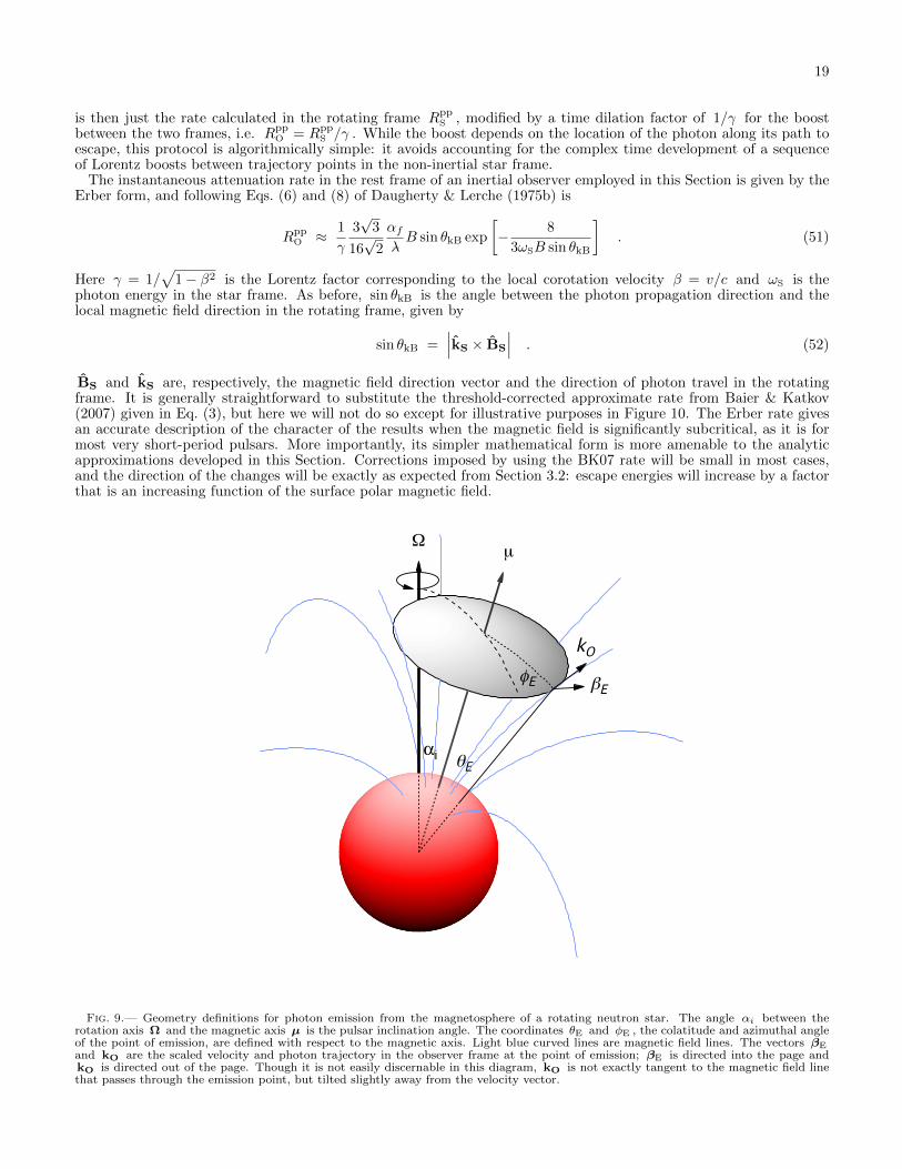
19

is then just the rate calculated in the rotating frame RppS , modified by a time dilation factor of 1/γ for the boost

between the two frames, i.e. RppO = Rpp

S /γ . While the boost depends on the location of the photon along its path toescape, this protocol is algorithmically simple: it avoids accounting for the complex time development of a sequenceof Lorentz boosts between trajectory points in the non-inertial star frame.

The instantaneous attenuation rate in the rest frame of an inertial observer employed in this Section is given by theErber form, and following Eqs. (6) and (8) of Daugherty & Lerche (1975b) is

RppO ≈ 1

γ

3√

3

16√

2

αfλ–B sin θkB exp

[− 8

3ωSB sin θkB

]. (51)

Here γ = 1/√

1− β2 is the Lorentz factor corresponding to the local corotation velocity β = v/c and ωS is thephoton energy in the star frame. As before, sin θkB is the angle between the photon propagation direction and thelocal magnetic field direction in the rotating frame, given by

sin θkB =∣∣∣kS × BS

∣∣∣ . (52)

BS and kS are, respectively, the magnetic field direction vector and the direction of photon travel in the rotatingframe. It is generally straightforward to substitute the threshold-corrected approximate rate from Baier & Katkov(2007) given in Eq. (3), but here we will not do so except for illustrative purposes in Figure 10. The Erber rate givesan accurate description of the character of the results when the magnetic field is significantly subcritical, as it is formost very short-period pulsars. More importantly, its simpler mathematical form is more amenable to the analyticapproximations developed in this Section. Corrections imposed by using the BK07 rate will be small in most cases,and the direction of the changes will be exactly as expected from Section 3.2: escape energies will increase by a factorthat is an increasing function of the surface polar magnetic field.

12

10

8

6

4

2

0

-2

-4

1086420-2-4-6

Wm

fE

qEαi

bE

kO

Fig. 9.— Geometry definitions for photon emission from the magnetosphere of a rotating neutron star. The angle αi between therotation axis Ω and the magnetic axis µ is the pulsar inclination angle. The coordinates θE and φE , the colatitude and azimuthal angleof the point of emission, are defined with respect to the magnetic axis. Light blue curved lines are magnetic field lines. The vectors βEand kO are the scaled velocity and photon trajectory in the observer frame at the point of emission; βE is directed into the page andkO is directed out of the page. Though it is not easily discernable in this diagram, kO is not exactly tangent to the magnetic field linethat passes through the emission point, but tilted slightly away from the velocity vector.

20

The geometry for the photon emission and opacity determination is illustrated in Fig. 9, where the magnetic dipoleaxis is inclined at an angle αi relative to the spin axis. In Cartesian coordinates with the z axis aligned with therotation axis and the xz plane defined as that containing the magnetic and rotation axes (so that for an orthogonalrotator with αi = 90 , the magnetic axis is aligned with the +x axis), the magnetic field (light blue lines in theFigure) at observer time tO = 0 is given by

BS(0) =

[Bx(0)By(0)Bz(0)

]=

3BpR3NS

2r3S

cosαi cos θS sin θS cosφS + sinαi(cos2 θS − 1

3

)cos θS sin θS sinφS

− sinαi cos θS sin θS cosφS + cosαi(cos2 θS − 1

3

) . (53)

By specifying a standard dipole µB(3 cos θS sin θS, 0, 3 cos2 θS − 1)/r3s , where µB = BpR

3NS/2 is the dipole moment,

this form is simply obtained by performing sequential rotations by φS about the z -axis and then αi about the y -axis,the latter of which can be described by the rotation matrix (subscript I denotes the magnetic inclination operator)

TI =

[cosαi 0 sinαi

0 1 0− sinαi 0 cosαi

]. (54)

Throughout this presentation, the subscript S denotes quantities in the star frame, and the angles in Eq. (53) relateto spherical polar coordinates in that frame. To derive the time development of this field BS(tO) as the star rotatesabout the z axis while a photon escapes the magnetosphere, we multiply this by the appropriate rotation matrix TΩ :

BS(tO) = TΩ ·BS(0) , TΩ(tO) =

[cos ΩtO − sin ΩtO 0sin ΩtO cos ΩtO 0

0 0 1

]. (55)

Here tO = s/c is the time an observer determines as the photon propagates a distance s after emission. In general,ΩtO 1 for the low altitude propagation zones where the greatest contributions to pair opacity are realized. It isimportant to note that BS represents the field vector in the instantaneous star frame at time tO , and must be boostedto the observer frame to define the complete electromagnetic field therein.

For initial conditions, it is assumed that the photon is emitted very nearly parallel to the magnetic field at the pointof emission in the star frame, as was done for the non-rotating case. The spherical polar coordinates at this pointare rS = rE , θS = θE , and φS = φE , as depicted in Figure 9. Normalizing this vector gives the direction of themagnetic field, which depends only on the colatitude and azimuthal angle, and can be obtained directly from Eq. (53).In the inertial observer (O) frame, the magnetic field direction vector and the photon trajectory vector will no longerbe parallel at the point of emission, due to relativistic aberration precipitated by the rotation. To specify this, the

corotation velocity−→βEc at the point of emission is needed. This depends only on the pulsar period and the 3D location

of the emission point, and is given by

−→βE =

2πrEcP

[ − sin θE sinφE

cosαi sin θE cosφE + sinαi cos θE0

]. (56)

For rE ≤ Pc/2π this dimensionless speed is always less than unity, except in the special case of emission at theequatorial light cylinder radius ( θE = π/2 , rE = Pc/2π ) and for an aligned rotator (αi = 0 ).

We now progress to the construction of the photon’s path in the reference frame of an inertial observer, which is astraight line in the absence of general relativistic corrections. Using the photon’s starting direction in the star frame,labelled by the unit vector kS,E ≡ BS,E derived from Eq. (53), and the instantaneous relative velocity between the

star frame and the observer frame of−→βEc , we can calculate the photon’s trajectory vector in the observer frame by

performing a Lorentz transformation on the photon’s 4-momentum in the star frame:

kO = ωS,E

BS,E + γE

[γE

γE + 1

(−→βE · BS,E

)− 1

]−→βE

. (57)

Following the dimensionless convention adopted throughout, the wave vector kO is scaled in terms of the inverseCompton wavelength mec/~ , as is its star frame counterpart kS below. In the star frame, the photon energy at thepoint of emission, ωS,E , is Doppler-shifted relative to the constant photon energy εO in the inertial observer frame:

ωS,E =εO

γE(1− BS,E ·

−→βE

) . (58)

This completes the specification of kO , which is a constant during propagation to infinity. When βE is small, as it isfor emission relatively close to the neutron star, all quantities that are second order in βE can be neglected, so thatEq. (57) approximately assumes the form

kO ≈ εO

BS,E −

−→βE

. (59)

21

The small-β approximation will be considered in more detail later in this Section and also in Appendix B, for thepurposes of generating useful analytic developments.

To compute the reaction rates in Eq. (51), one needs the direction of photon travel in the star frame, where the path iscurved, so that the value of sin θkB can be determined. This direction can be obtained at each point by transformingkO back to the star frame, using the instantaneous β and γ at each point. This transformation preserves the

component of momentum k⊥ = kO−(kO · β

)β orthogonal to the boost, but stretches/contracts the component along

~β via the relation kS · β = γ(kO · β + β |kO|

), similar to the protocol adopted for Eq. (57). The momentum vectors

of the photon in the two frames at each position along the trajectory are then given by the conjugate relations

kO = kS + γ

[γ

γ + 1

(−→β · kS

)− |kS|

]−→β ,

(60)

kS = kO + γ

[γ

γ + 1

(−→β · kO

)+ |kO|

]−→β .

The first equation in this couplet is just an extension of Eq. (57) to arbitrary altitudes using−→βE →

−→β and ωS,EBS,E →

kS . To maintain constancy of kO along the entire trajectory, |kS| = ωS adjusts its value at each point via the

aberration relation γωS

(1 − kS ·

−→β)

= εO that is the analog of Eq. (58). The second relation of this pair is just

the inversion of the first, under the interchange S↔O and also−→β → −

−→β ; it is that desired for the computation

of sin θkB . Observe that forming the dot product ω2S = |kS|2 can be used to derive the inverse aberration relation

ωS = γεO(1 + kO ·−→β ) . Note that in the absence of rotation (P →∞ , β → 0 ), one recovers kS = kO = εOBS,E , as

expected.

Calculating the corotation velocity−→β at every point along the photon trajectory is straightforward. The straight-

line photon path in the observer frame is given simply by

rO = rE + skO, (61)

where s = ct is the distance traveled, and rE is the emission point. This is conveniently expressed in sphericalcoordinates about the rotation axis, still as a function of s :

[rO(s)θO(s)φO(s)

]=

√r2E + s2 + 2srE · kO

cos−1 rE,z + skO,z

rO(s)

tan−1 rE,y + skO,y

rE,x + skO,x

. (62)

In this form, the coupling between the rotational phase φO and the trajectory is simply displayed. In general, we

do not restrict the emission plane to zero phase φO , i.e. kO , BS,E and−→βE are not coplanar. The local corotation

velocity is then given as a function of s in Cartesian coordinates by

−→β (s) =

rO(s)Ω

csin θO

[− sinφO(s)cosφO(s)

0

]. (63)

Since kO in Eq. (57) is also expressible in Cartesian coordinates, the determination of kS via Eq. (60) is routine.The remaining ingredient needed for the determination of the pair conversion rates is the second vector for the

calculation of sin θkB in Eq. (52), namely the magnetic field vector in the star frame, BS(s) . Given the simple dipolarform in the star frame, the only complexity is encapsulated in the conversion of the straight-line trajectory in theinertial observer frame into star frame coordinates, where the path is curved. Given coordinates xO, yO, zO in theobserver frame, obtained from Eq. (61), the photon trajectory in the star frame can be expressed via

ctSxS

ySzS

= L ·

ctOxO

yOzO

for L =

γ γβx γβy 0

γβx 1 + (γ − 1)β2x

β2 (γ − 1)βxβyβ2 0

γβy (γ − 1)βxβyβ2 1 + (γ − 1)

β2y

β2 0

0 0 0 1

(64)

being a standard Lorentz transformation matrix, L = L(s) . Since the boost is purely in the xy direction and s = ctO ,

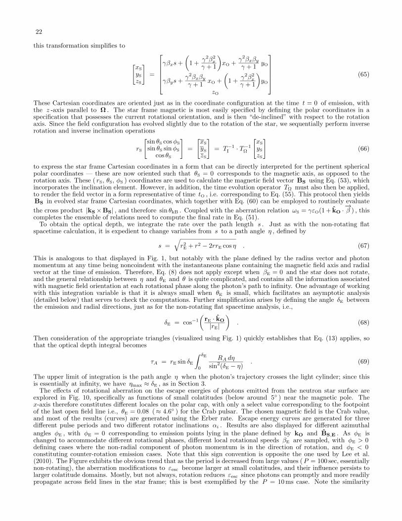
22

this transformation simplifies to

[xS

ySzS

]=

γβxs+

(1 +

γ2β2x

γ + 1

)xO +

γ2βxβyγ + 1

yO

γβys+γ2βxβyγ + 1

xO +

(1 +

γ2β2x

γ + 1

)yO

zO

(65)

These Cartesian coordinates are oriented just as in the coordinate configuration at the time t = 0 of emission, withthe z -axis parallel to Ω . The star frame magnetic is most easily specified by defining the polar coordinates in aspecification that possesses the current rotational orientation, and is then “de-inclined” with respect to the rotationaxis. Since the field configuration has evolved slightly due to the rotation of the star, we sequentially perform inverserotation and inverse inclination operations

rS

[sin θS cosφS

sin θS sinφS

cos θS

]=

[xS

ySzS

]= T−1

I · T−1Ω

[xS

ySzS

](66)

to express the star frame Cartesian coordinates in a form that can be directly interpreted for the pertinent sphericalpolar coordinates — these are now oriented such that θS = 0 corresponds to the magnetic axis, as opposed to therotation axis. These ( rS, θS, φS ) coordinates are used to calculate the magnetic field vector BS using Eq. (53), whichincorporates the inclination element. However, in addition, the time evolution operator TΩ must also then be applied,to render the field vector in a form representative of time tO , i.e. corresponding to Eq. (55). This protocol then yieldsBS in evolved star frame Cartesian coordinates, which together with Eq. (60) can be employed to routinely evaluate

the cross product |kS×BS| , and therefore sin θkB . Coupled with the aberration relation ωS = γεO(1 + kO ·−→β ) , this

completes the ensemble of relations need to compute the final rate in Eq. (51).To obtain the optical depth, we integrate the rate over the path length s . Just as with the non-rotating flat

spacetime calculation, it is expedient to change variables from s to a path angle η , defined by

s =√r2E + r2 − 2rrE cos η . (67)

This is analogous to that displayed in Fig. 1, but notably with the plane defined by the radius vector and photonmomentum at any time being noncoindent with the instantaneous plane containing the magnetic field axis and radialvector at the time of emission. Therefore, Eq. (8) does not apply except when βE = 0 and the star does not rotate,and the general relationship between η and θE and θ is quite complicated, and contains all the information associatedwith magnetic field orientation at each rotational phase along the photon’s path to infinity. One advantage of workingwith this integration variable is that it is always small when θE is small, which facilitates an asymptotic analysis(detailed below) that serves to check the computations. Further simplification arises by defining the angle δE betweenthe emission and radial directions, just as for the non-rotating flat spacetime analysis, i.e.,

δE = cos−1

(rE · kO

|rE|

). (68)

Then consideration of the appropriate triangles (visualized using Fig. 1) quickly establishes that Eq. (13) applies, sothat the optical depth integral becomes

τA = rE sin δE

∫ δE

0

RA dηsin2(δE − η)

. (69)

The upper limit of integration is the path angle η when the photon’s trajectory crosses the light cylinder; since thisis essentially at infinity, we have ηmax ≈ δE , as in Section 3.

The effects of rotational aberration on the escape energies of photons emitted from the neutron star surface areexplored in Fig. 10, specifically as functions of small colatitudes (below around 5 ) near the magnetic pole. Thex-axis therefore constitutes different locales on the polar cap, with only a select value corresponding to the footpointof the last open field line i.e., θE = 0.08 (≈ 4.6 ) for the Crab pulsar. The chosen magnetic field is the Crab value,and most of the results (curves) are generated using the Erber rate. Escape energy curves are generated for threedifferent pulse periods and two different rotator inclinations αi . Results are also displayed for different azimuthalangles φE , with φE = 0 corresponding to emission points lying in the plane defined by kO and BS,E . As φE ischanged to accommodate different rotational phases, different local rotational speeds βE are sampled, with φE > 0defining cases where the non-radial component of photon momentum is in the direction of rotation, and φE < 0constituting counter-rotation emission cases. Note that this sign convention is opposite the one used by Lee et al.(2010). The Figure exhibits the obvious trend that as the period is decreased from large values (P = 100 sec, essentiallynon-rotating), the aberration modifications to εesc become larger at small colatitudes, and their influence persists tolarger colatitude domains. Mostly, but not always, rotation reduces εesc since photons can promptly and more readilypropagate across field lines in the star frame; this is best exemplified by the P = 10 ms case. Note the similarity

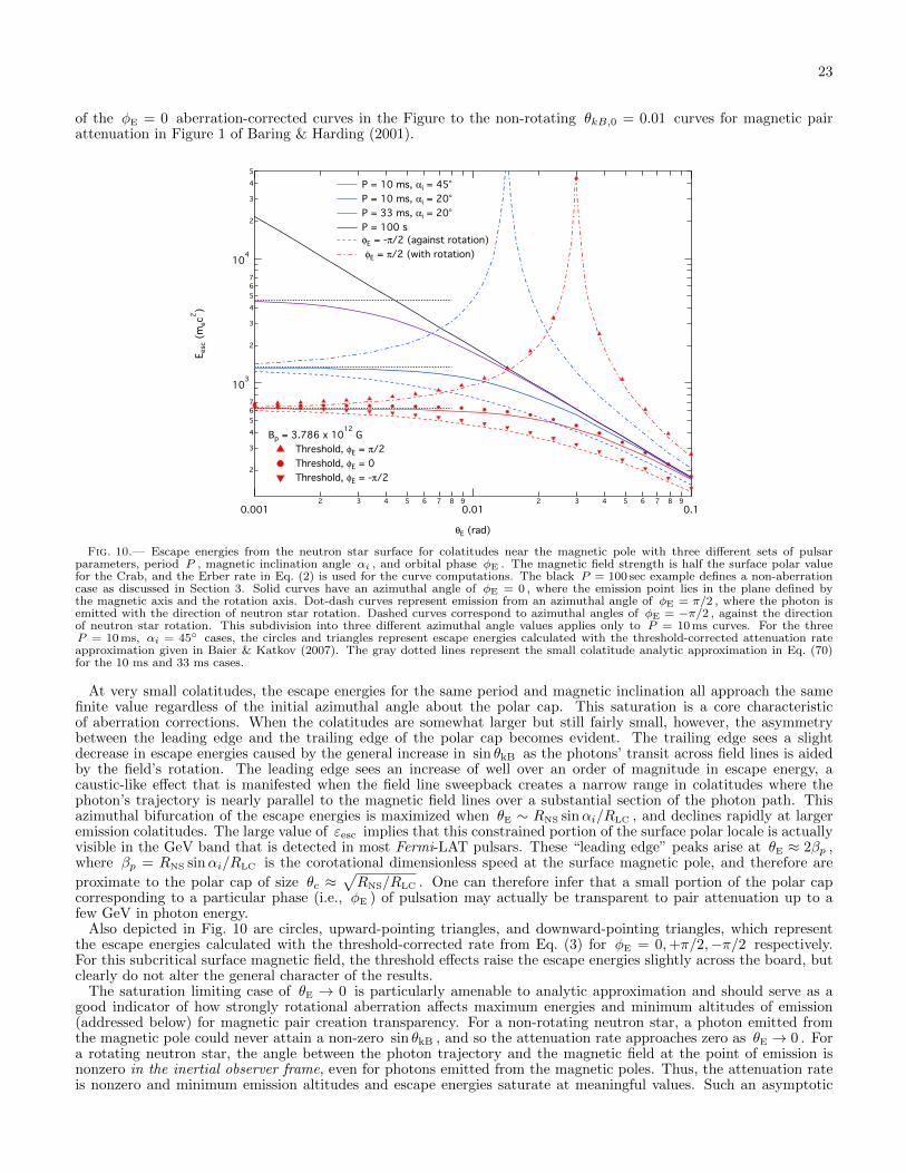
23

of the φE = 0 aberration-corrected curves in the Figure to the non-rotating θkB,0 = 0.01 curves for magnetic pairattenuation in Figure 1 of Baring & Harding (2001).

2

3

4

5

67

103

2

3

4

5

67

104

2

3

4

5

Eesc

(m

ec

2)

0.0012 3 4 5 6 7 8 9

0.012 3 4 5 6 7 8 9

0.1

θE (rad)

P = 10 ms, αi = 45¡

P = 10 ms, αi = 20¡

P = 33 ms, αi = 20¡

P = 100 s

φE = -π/2 (against rotation)

φE = π/2 (with rotation)

Bp = 3.786 x 1012

G

Threshold, φE = π/2

Threshold, φE = 0

Threshold, φE = -π/2

Fig. 10.— Escape energies from the neutron star surface for colatitudes near the magnetic pole with three different sets of pulsarparameters, period P , magnetic inclination angle αi , and orbital phase φE . The magnetic field strength is half the surface polar valuefor the Crab, and the Erber rate in Eq. (2) is used for the curve computations. The black P = 100 sec example defines a non-aberrationcase as discussed in Section 3. Solid curves have an azimuthal angle of φE = 0 , where the emission point lies in the plane defined bythe magnetic axis and the rotation axis. Dot-dash curves represent emission from an azimuthal angle of φE = π/2 , where the photon isemitted with the direction of neutron star rotation. Dashed curves correspond to azimuthal angles of φE = −π/2 , against the directionof neutron star rotation. This subdivision into three different azimuthal angle values applies only to P = 10 ms curves. For the threeP = 10 ms, αi = 45 cases, the circles and triangles represent escape energies calculated with the threshold-corrected attenuation rateapproximation given in Baier & Katkov (2007). The gray dotted lines represent the small colatitude analytic approximation in Eq. (70)for the 10 ms and 33 ms cases.

At very small colatitudes, the escape energies for the same period and magnetic inclination all approach the samefinite value regardless of the initial azimuthal angle about the polar cap. This saturation is a core characteristicof aberration corrections. When the colatitudes are somewhat larger but still fairly small, however, the asymmetrybetween the leading edge and the trailing edge of the polar cap becomes evident. The trailing edge sees a slightdecrease in escape energies caused by the general increase in sin θkB as the photons’ transit across field lines is aidedby the field’s rotation. The leading edge sees an increase of well over an order of magnitude in escape energy, acaustic-like effect that is manifested when the field line sweepback creates a narrow range in colatitudes where thephoton’s trajectory is nearly parallel to the magnetic field lines over a substantial section of the photon path. Thisazimuthal bifurcation of the escape energies is maximized when θE ∼ RNS sinαi/RLC , and declines rapidly at largeremission colatitudes. The large value of εesc implies that this constrained portion of the surface polar locale is actuallyvisible in the GeV band that is detected in most Fermi-LAT pulsars. These “leading edge” peaks arise at θE ≈ 2βp ,where βp = RNS sinαi/RLC is the corotational dimensionless speed at the surface magnetic pole, and therefore are

proximate to the polar cap of size θc ≈√RNS/RLC . One can therefore infer that a small portion of the polar cap

corresponding to a particular phase (i.e., φE ) of pulsation may actually be transparent to pair attenuation up to afew GeV in photon energy.

Also depicted in Fig. 10 are circles, upward-pointing triangles, and downward-pointing triangles, which representthe escape energies calculated with the threshold-corrected rate from Eq. (3) for φE = 0,+π/2,−π/2 respectively.For this subcritical surface magnetic field, the threshold effects raise the escape energies slightly across the board, butclearly do not alter the general character of the results.

The saturation limiting case of θE → 0 is particularly amenable to analytic approximation and should serve as agood indicator of how strongly rotational aberration affects maximum energies and minimum altitudes of emission(addressed below) for magnetic pair creation transparency. For a non-rotating neutron star, a photon emitted fromthe magnetic pole could never attain a non-zero sin θkB , and so the attenuation rate approaches zero as θE → 0 . Fora rotating neutron star, the angle between the photon trajectory and the magnetic field at the point of emission isnonzero in the inertial observer frame, even for photons emitted from the magnetic poles. Thus, the attenuation rateis nonzero and minimum emission altitudes and escape energies saturate at meaningful values. Such an asymptotic

24

result can be determined by following a procedure much like the one discussed at some length in Section 3.1. Oneobtains the following approximation for the optical depth at θE = 0 (with Bp scaled by Bcr ):

τA ≈36√

3218

αfRNS

λ–h2

√πε

(BpRNS sinαi

RLC

)3/2

exp

− 212h2RLC

35εBpRNS sinαi

, (70)

where h = rE/RNS , and RLC = Pc/2π expresses the pulsar period. The details of this development can be found inAppendix B. Setting this equal to unity, we can solve for εesc :

εesc =212 h2

35Bpβp

[loge

αfRNS

λ–+

12

logeεesc

h4 +32

logeBpβp − 5.34

]−1

. (71)

In this expression, βp = RNS sinαi/RLC is again the dimensionless rotation speed at the surface polar location in itscircular path, and is the key parameter defining the scale of rotational influences. Comparison with the correspondingnon-rotating result in Eq. (20) indicates that here βp plays a role equivalent to the footpoint colatitude θf there,because both βp and θf are proportional to the angle between the photon momentum vector and the radial directionat the neutron star surface. Accordingly, aberration modifications should diminish for these low altitude emissionconsiderations when θE substantially exceeds βp , and all cases should coalesce to the static (P →∞ ), flat spacetimecurve: this circumstance is clearly evident in Fig. 10. Observe that the choice of azimuthal angle φE provides asecond-order correction O(θ2

E) when at extremely small colatitudes above the magnetic pole, and so does not appearin these leading-order asymptotic formulae.

The transcendental Eq. (71) must be solved numerically, in general, though the weak dependence on εesc in thelogarithmic term, when neglected, permits approximate analytic solution for the escape energy. Numerical results arediplayed as the gray dashed line saturation asymptotes in Fig. 10, for the case of surface emission (h = 1 ) and periods10 ms and 33 ms. One can immediately see that to leading order, as θE → 0 , since εesc ∝ β−1

p , one should expectto see εesc ∝ P and εesc ∝ 1/ sinαi : these dependences are clearly exhibited in the Figure. Moreover, the computednumerical εesc curves asymptotically approach the solutions of Eq. (71) as θE → 0 .

8

6

4

2

r min (

NS r

adii)

806040200

θE (deg)

2.5

2.0

1.5

1.0

543210

Bp = Bcrab, ω = 1 GeV

P = 10 ms, αi = 45¡, φE = 0

P = 10 ms, αi = 45¡, φE = -π/2

P = 10 ms, αi = 45¡, φE = +π/2

P = 10 ms, αi = 20¡

P = 100 s

Fig. 11.— Minimum altitudes of emission from the magnetic pole to the magnetic equator, for different sets of pulsar parameters. TheCrab field value was adopted. As in Fig. 10, the dot-dash curves represent photons emitted on the leading side of the magnetic pole(evincing non-monotonic behavior of rmin with θE – see inset), and dashed curves represent photons emitted on the trailing side of thepole. The gray dotted lines in the inset represent the zero-colatitude analytic approximation in Eq. (70).

Fig. 11 shows the effect of rotational aberration on the minimum altitudes of emission of 1 GeV photons; similarbehavior is exhibited for other test photon energies. The surface polar magnetic field is again chosen to be the Crabvalue. Such altitude bounds are plotted as functions of emission colatitude, and except for very close to the pole, aregenerally well below the altitude of the last open field line. The red curve is a pulsar with a period of 100 sec, whereaberration effects are minimal. The blue and green curves represent photons emitted from an azimuthal angle of zerofor pulsars with periods of 10 seconds and inclination angles of 20 and 45 degrees, respectively. Green dotted anddashed lines represent photons emitted from the leading side of the magnetic pole (with the direction of rotation) andthe trailing side (against the direction of rotation). Gray dashed lines again represent the θE = 0 limit calculated

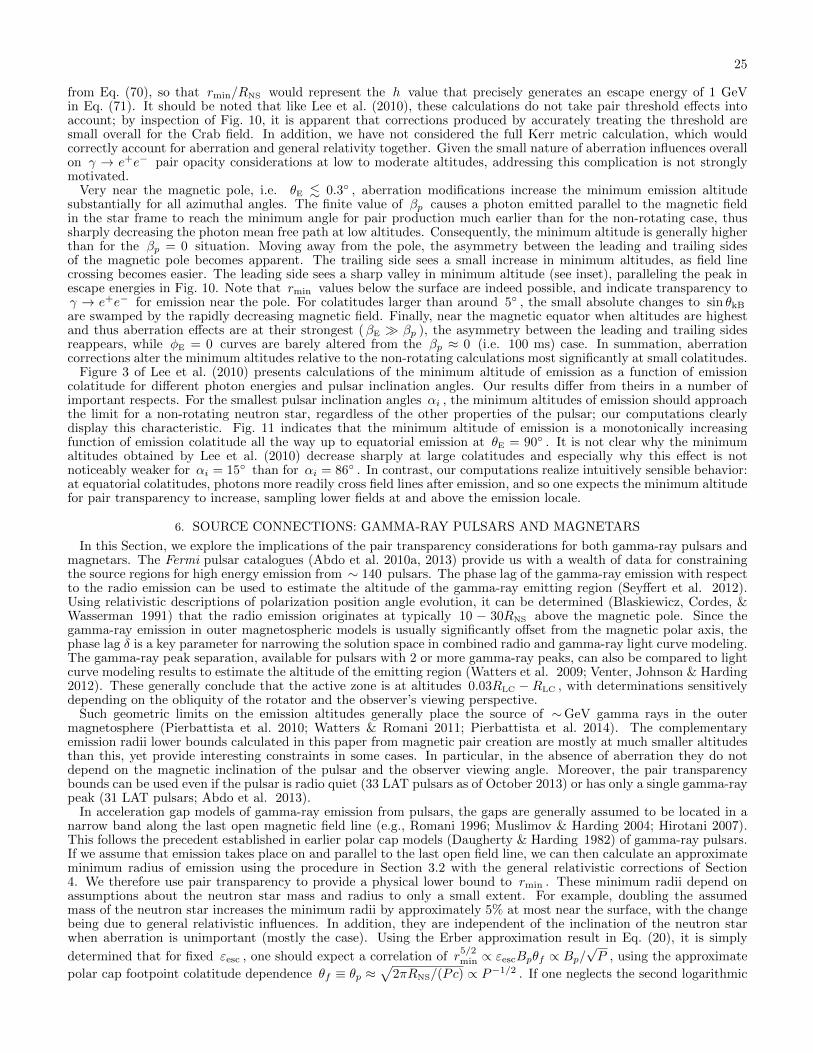
25

from Eq. (70), so that rmin/RNS would represent the h value that precisely generates an escape energy of 1 GeVin Eq. (71). It should be noted that like Lee et al. (2010), these calculations do not take pair threshold effects intoaccount; by inspection of Fig. 10, it is apparent that corrections produced by accurately treating the threshold aresmall overall for the Crab field. In addition, we have not considered the full Kerr metric calculation, which wouldcorrectly account for aberration and general relativity together. Given the small nature of aberration influences overallon γ → e+e− pair opacity considerations at low to moderate altitudes, addressing this complication is not stronglymotivated.

Very near the magnetic pole, i.e. θE . 0.3 , aberration modifications increase the minimum emission altitudesubstantially for all azimuthal angles. The finite value of βp causes a photon emitted parallel to the magnetic fieldin the star frame to reach the minimum angle for pair production much earlier than for the non-rotating case, thussharply decreasing the photon mean free path at low altitudes. Consequently, the minimum altitude is generally higherthan for the βp = 0 situation. Moving away from the pole, the asymmetry between the leading and trailing sidesof the magnetic pole becomes apparent. The trailing side sees a small increase in minimum altitudes, as field linecrossing becomes easier. The leading side sees a sharp valley in minimum altitude (see inset), paralleling the peak inescape energies in Fig. 10. Note that rmin values below the surface are indeed possible, and indicate transparency toγ → e+e− for emission near the pole. For colatitudes larger than around 5 , the small absolute changes to sin θkB

are swamped by the rapidly decreasing magnetic field. Finally, near the magnetic equator when altitudes are highestand thus aberration effects are at their strongest (βE βp ), the asymmetry between the leading and trailing sidesreappears, while φE = 0 curves are barely altered from the βp ≈ 0 (i.e. 100 ms) case. In summation, aberrationcorrections alter the minimum altitudes relative to the non-rotating calculations most significantly at small colatitudes.

Figure 3 of Lee et al. (2010) presents calculations of the minimum altitude of emission as a function of emissioncolatitude for different photon energies and pulsar inclination angles. Our results differ from theirs in a number ofimportant respects. For the smallest pulsar inclination angles αi , the minimum altitudes of emission should approachthe limit for a non-rotating neutron star, regardless of the other properties of the pulsar; our computations clearlydisplay this characteristic. Fig. 11 indicates that the minimum altitude of emission is a monotonically increasingfunction of emission colatitude all the way up to equatorial emission at θE = 90 . It is not clear why the minimumaltitudes obtained by Lee et al. (2010) decrease sharply at large colatitudes and especially why this effect is notnoticeably weaker for αi = 15 than for αi = 86 . In contrast, our computations realize intuitively sensible behavior:at equatorial colatitudes, photons more readily cross field lines after emission, and so one expects the minimum altitudefor pair transparency to increase, sampling lower fields at and above the emission locale.

6. SOURCE CONNECTIONS: GAMMA-RAY PULSARS AND MAGNETARS

In this Section, we explore the implications of the pair transparency considerations for both gamma-ray pulsars andmagnetars. The Fermi pulsar catalogues (Abdo et al. 2010a, 2013) provide us with a wealth of data for constrainingthe source regions for high energy emission from ∼ 140 pulsars. The phase lag of the gamma-ray emission with respectto the radio emission can be used to estimate the altitude of the gamma-ray emitting region (Seyffert et al. 2012).Using relativistic descriptions of polarization position angle evolution, it can be determined (Blaskiewicz, Cordes, &Wasserman 1991) that the radio emission originates at typically 10 − 30RNS above the magnetic pole. Since thegamma-ray emission in outer magnetospheric models is usually significantly offset from the magnetic polar axis, thephase lag δ is a key parameter for narrowing the solution space in combined radio and gamma-ray light curve modeling.The gamma-ray peak separation, available for pulsars with 2 or more gamma-ray peaks, can also be compared to lightcurve modeling results to estimate the altitude of the emitting region (Watters et al. 2009; Venter, Johnson & Harding2012). These generally conclude that the active zone is at altitudes 0.03RLC − RLC , with determinations sensitivelydepending on the obliquity of the rotator and the observer’s viewing perspective.

Such geometric limits on the emission altitudes generally place the source of ∼GeV gamma rays in the outermagnetosphere (Pierbattista et al. 2010; Watters & Romani 2011; Pierbattista et al. 2014). The complementaryemission radii lower bounds calculated in this paper from magnetic pair creation are mostly at much smaller altitudesthan this, yet provide interesting constraints in some cases. In particular, in the absence of aberration they do notdepend on the magnetic inclination of the pulsar and the observer viewing angle. Moreover, the pair transparencybounds can be used even if the pulsar is radio quiet (33 LAT pulsars as of October 2013) or has only a single gamma-raypeak (31 LAT pulsars; Abdo et al. 2013).

In acceleration gap models of gamma-ray emission from pulsars, the gaps are generally assumed to be located in anarrow band along the last open magnetic field line (e.g., Romani 1996; Muslimov & Harding 2004; Hirotani 2007).This follows the precedent established in earlier polar cap models (Daugherty & Harding 1982) of gamma-ray pulsars.If we assume that emission takes place on and parallel to the last open field line, we can then calculate an approximateminimum radius of emission using the procedure in Section 3.2 with the general relativistic corrections of Section4. We therefore use pair transparency to provide a physical lower bound to rmin . These minimum radii depend onassumptions about the neutron star mass and radius to only a small extent. For example, doubling the assumedmass of the neutron star increases the minimum radii by approximately 5% at most near the surface, with the changebeing due to general relativistic influences. In addition, they are independent of the inclination of the neutron starwhen aberration is unimportant (mostly the case). Using the Erber approximation result in Eq. (20), it is simply

determined that for fixed εesc , one should expect a correlation of r5/2min ∝ εescBpθf ∝ Bp/

√P , using the approximate

polar cap footpoint colatitude dependence θf ≡ θp ≈√

2πRNS/(Pc) ∝ P−1/2 . If one neglects the second logarithmic

26

(Bp -dependent) term inside the parentheses in Eq. (20), this flat space-time correlation is approximately

rmin

RNS≈ 0.037ε2/5

esc 102σIG/5 , σIG = log10

(B12√P

), (72)

where the unscaled polar field is Bp = B121012 Gauss, and we set RNS = 106 cm. For the purposes of this discussion,

here we adopt the relation Bp ≈ 6.4 × 1019√P P for the unscaled field, which corresponds to the vacuum magnetic

dipole moment µ = BpR3NS/2 (Shapiro & Teukolsky 1983; Usov & Melrose 1995), and is twice the conventional choice

of Manchester & Taylor (1977) that is applicable to the equatorial surface field. Note that non-dipolar contributions

and plasma loading of the magnetosphere modify such inferences of pulsar surface fields from P and P .Fig. 12 shows the minimum radii of emission for the pulsars listed in the second Fermi catalog, plotted against σIG ,

a proxy for the logarithm of Bp/√P . These minimum radii are calculated using a test photon energy that is twice the

cutoff energy Ec published in the catalog paper (Abdo et al. 2013). The choice of 2Ec does not exactly represent thehighest energy photons detected from the source, but is slightly above the energy where the νFν is at a maximum,modulo a factor that depends on the power-law spectral index below the cutoff. The cutoff energies from the fits rangefrom 0.4 to 5.9 GeV for the sources where spectral fitting produces significant determinations of Ec ; the Crab pulsaris an exceptional case that will be isolated below. The handful of pulsars with poor spectral fits in Table 9 of Abdo etal. (2013) are not included in this analysis.

10

8

6

4

2

Min

imum

Alt

itude, r m

in/r N

S

2.52.01.51.00.50.0

σIG = Log10[B12 (1012

G) ] - 1/2 Log10 [P (sec)]

Crab

Vela

Fig. 12.— Minimum emission radii for a selection (see text) of young pulsars among the 117 pulsars in the second Fermi pulsar catalog

(Abdo et al. 2013). The minimum radius in neutron star radii is plotted against a scaling of the logarithm of B12/√P . This couples

directly to the dependence suggested in Eq. (72) for flat space-time, an indication of which is provided by the black curve, which represents

rmin/RNS = 4/3× 102σIG/5 . These minimum radii are found by solving τ(rE, εc) = 1 for rE , using twice the exponential cutoff energiesEc measured by Fermi-LAT (Abdo et al. 2013), and assuming that emission takes place on the last open field line. If the same calculationis done for the VERITAS detection of the Crab pulsar at 120 GeV, we get a minimum radius of 20RNS , while the MAGIC claim of pulsedemission up to 350 − 400 GeV would raise the bound to rmin ∼ 31RNS ; both far exceed the minimum radius of 7.25RNS obtained fromthe Fermi cutoff energy.

Pulsars with magnetic fields too low for magnetic pair creation to play a significant role in propagation of GeV-bandphotons in their magnetospheres, including nearly all millisecond pulsars, are not constrained at all by this technique;their pair attenuation “minimum radii” are not only inside the neutron star, but inside the Schwarzschild radius, andtherefore not meaningful. As an example, PSR B1821-24 in the globular cluster M28, with its period P = 3.05 ms andperiod derivative P = 1.62×10−18 sec sec−1, possesses the highest known spin-down luminosity of any MSP (Johnson,et al. 2013). Its surface polar field is Bp ≈ 4.5 × 109 Gauss, i.e. approximately 10−4Bcr . One can infer from Fig. 3that its polar cap angle of ≈ 15 would then yield an escape energy of around 30 GeV, a factor of 100 higher than

27

for the Bp = 0.01 case illustrated therein. This εesc is above the turnover energy Ec ∼ 6 GeV determined in thepulsed Fermi-LAT data in Johnson, et al. (2013), so that pair transparency for all photons detected by the LAT canbe presumed at altitudes above the surface.

The rmin values in Fig. 12 display a general increase with σIG , but considerable scatter. The relation in Eq. (72)is schematically represented in the Figure via the black curve rmin/RNS = 4/3× 102σIG/5 , corresponding to a value ofεesc ≈ 4× 103 (i.e., 2.0 GeV) in Eq. (72). This defines the general character of the minimum altitude calculations, sothat the scatter expresses the distribution of Ec values in the Fermi pulsar spectral database. The point in the topright corner, with an rmin value over 10RNS , is for PSR J1119-6127, a high-field pulsar with a surface polar field wellabove the quantum critical value. For the Crab and Vela pulsars, the minimum radii calculated using the Fermi-LATcutoff energies are indicated on the plot. If one performs the same calculation for the VERITAS detection of pulsedemission from the Crab pulsar at 120 GeV (Aliu et al. 2011), the minimum emission radius for those 120 GeV photonsis approximately 20RNS . Even more interestingly, the MAGIC experiment has displayed evidence of pulsed emissionfrom the Crab up to 350–400 GeV (see Fig. 4 of Aleksic et al. 2012), for which the rmin determination increasesto around 31RNS , or approximately 0.2RLC . This is a profound constraint that impacts the discussion of slot gapversus outer gap models of the Crab, and is completely independent of altitude inferences from pulse profile geometricanalyses. Observe that if the lower spin-down field estimate of Manchester & Taylor (1977) is adopted, this bounddrops only to rmin ≈ 23RNS ≈ 0.15RLC , still offering an important constraint. Note also that at these altitudes, onemight expect rotational aberration to be influential, perhaps more so in the trailing edge of emission. By inspectionof the altitude bound in Fig. 11 for lower energy (GeV) photons, we anticipate that aberration will provide at most amodest modification to this rmin ∼ 0.2RLC determination.

To provide a striking contrast to this case, the same analysis can be performed for the softest Fermi-LAT gamma-raypulsar, PSR J1513-5908 (B1509-58), whose signal extends only out to around 230 MeV. This high-field pulsar has aperiod of 151 ms, is fairly faint in the LAT band (Abdo et al. 2010d) and is detected by AGILE (Pilia et al. 2010),also out to around 200-300 MeV. It was not detected by EGRET on the Compton Gamma-Ray Observatory, but wasseen by COMPTEL at energies below 30 MeV (Kuiper et al. 1999). Using 230 MeV to set εesc , we infer a minimumemission radius of approximately 2.3RNS . While this is not constraining for slot gap and outer gap models, it is ofsignificant interest that it is somewhat above the surface. The broad pulse profile (Abdo et al. 2010d) implies that amore substantial range of emission altitudes can be accommodated than is typical for gamma-ray pulsars. Moreover,the fact that one of the gamma-ray peaks very slightly leads the radio pulse peak (Abdo et al. 2010d) may be anindicator of a polar cap type component to the pulsar’s signal. Early interpretation of the EGRET upper limitsargued for the action of photon splitting in the strong fields near the surface of PSR J1513-5908 (Harding, Baring &Gonthier 1997), which has Bp = 3.1 × 1013 Gauss. This suggestion was predicated on the contention that polar capmodels could account for the emission in this pulsar, and required the gamma-ray attenuation by the splitting processto arise proximate to the polar cap. The pair transparency altitude bound computed here indicates that the magneticfield local to the emission of ∼ 230 MeV photons is less than ∼ 2.4 × 1012 Gauss, a lower field domain that stronglyinhibits photon splitting opacity (e.g., Baring & Harding 2001) in a neutron star magnetosphere.

It should be noted that if the magnetic field includes higher-order multipole components, as in Arons & Scharlemann(1979), the minimum emission radii calculated using this technique will change. The addition of a toroidal componentto the magnetic field will increase the magnetic field magnitude and decrease the field line radius of curvature in mostof the inner magnetosphere, which will make it easier for photons to transit across field lines and thereby enhance theattenuation of photons by magnetic pair creation. This must then be compensated by moving the emission regions tohigher altitudes where the field is lower. For this case, therefore, our rmin estimates serve as conservative lower limits.An off-center dipole magnetic field (e.g., Harding & Muslimov 2011) will introduce an asymmetry in field magnitudeand radius of curvature, which will bring rmin down on the “stretched” side and raise it up on the “compressed”side. This provides a modest range of minimum altitudes so that our computations serve as approximate guides. Weanticipate that the modifications introduced by offset dipolar morphology are tantamount to selecting a field line ofslightly different footpoint colatitude from that for the last open field line in a true dipole field; interpretation of thenumerical results presented here can then be adjusted accordingly.

The second observational context considered here concerns magnetars, namely soft gamma repeaters (SGRs) andanomalous X-ray pulsars (AXPs). With their supercritical fields, these energetic cousins of pulsars possess steadypulsed emission that is very different from that of gamma-ray pulsars. They have prominent thermal X-ray emissionbelow 10 keV, and virtually equally luminous hard X-ray emission (e.g., Kuiper, Hermsen & Mendez 2004; Goetz,et al. 2006; den Hartog, Kuiper, Hermsen, et al. 2008; den Hartog, Kuiper & Hermsen 2008) that is well-describedby power-law tails. These flat tails cannot extend beyond energies of a few hundred keV due to constraining upperlimits obtained by the COMPTEL instrument on the Compton Gamma-Ray Observatory. A prominent model for thetail emission is that it is due to inverse Compton scattering of surface thermal X-rays by relativistic electrons in thestrong fields of the inner magnetosphere (Baring & Harding 2007; Nobili, Turolla & Zane 2008; Baring, Wadiasingh& Gonthier 2011; Beloborodov 2013). Such emission should then be subject to the magnetic pair attenuation that isthe focus of this paper. Here we determine the energy ranges for which pair opacity should strongly attenuate the tailspectra. Magnetars also exhibit flaring episodes, ranging in luminosity up to the giant flares seen in three soft gammarepeaters. This emission also does not extend beyond about 1 MeV. A comprehensive observational and theoreticalsummary of magnetars can be found in Mereghetti (2008).

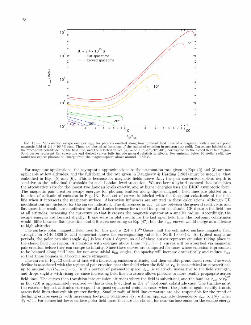
28

100

101

102

103

104

Em

ax (

MeV

)

12 3 4 5 6 7 8 9

102 3 4 5 6 7 8 9

100

Re/RNS

Bp = 2.4 x 1015

G

Flat spacetime

Curved spacetime

5¼

10¼

20¼30¼40¼

Fig. 13.— Pair creation escape energies εesc for photons emitted along four different field lines of a magnetar with a surface polarmagnetic field of 2.4× 1015 Gauss. These are plotted as functions of the radius of emission in neutron star radii. Curves are labeled withthe “footpoint colatitude” of the field line, and the selected values ( θf = 5, 10, 20, 30, 40 ) correspond to the closed field line region.Solid curves represent flat spacetime and dashed curves fully include general relativistic effects. For emission below 10 stellar radii, onewould not expect photons to emerge from the magnetosphere above around 10 MeV.

For magnetar applications, the asymptotic approximations to the attenuation rate given in Eqs. (2) and (3) are notapplicable at low altitudes, and the full form of the rate given in Daugherty & Harding (1983) must be used, i.e. thatembodied in Eqs. (5) and (6). This is because for magnetic fields above Bcr , the pair conversion optical depth issensitive to the individual thresholds for each Landau level transition. We use here a hybrid protocol that calculatesthe attenuation rate for the lowest two Landau levels exactly, and at higher energies uses the BK07 asymptotic form.The magnetic pair creation escape energies for photons emitted along dipole magnetic field lines are plotted as afunction of altitude of emission in Fig. 13. Each set of curves is labeled with the footpoint colatitude of the fieldline when it intersects the magnetar surface. Aberration influences are omitted in these calculations, although GRmodifications are included for the curves indicated. The differences in εesc values between the general relativistic andflat spacetime results are manifested for all altitudes because for a fixed footpoint colatitude, GR distorts the field lineat all altitudes, increasing the curvature so that it crosses the magnetic equator at a smaller radius. Accordingly, theescape energies are lowered slightly. If one were to plot results for the last open field line, the footpoint colatitudeswould differ between flat spacetime and GR cases according to Eq. (47), but the εesc curves would merge at moderateto high altitudes.

The surface polar magnetic field used for this plot is 2.4 × 1015 Gauss, half the estimated surface magnetic fieldstrength for SGR 1806-20 and somewhat above the corresponding value for SGR 1900+14. At typical magnetarperiods, the polar cap size (angle θp ) is less than 1 degree, so all of these curves represent emission taking place inthe closed field line region. All photons with energies above these τ(εesc) = 1 curves will be absorbed via magneticpair creation before they can escape to infinity. Since these curves are computed for cases where emission is presumedto be beamed along field lines, for non-zero initial θkB angles, the opacity will increase dramatically and reduce εesc

so that these bounds will become more stringent.The curves in Fig. 13 decline at first with increasing emission altitude, and then exhibit pronounced rises. The weak

decline is associated with the regime of pair creation near threshold when the field at rE is near-critical or supercritical,up to around rE/RNS ∼ 3− 6 . In this portion of parameter space, εesc is relatively insensitive to the field strength,and drops slightly with rising rE since increasing field line curvature allows photons to more readily propagate across

field lines. The curves then transition into emission altitudes where the field is subcritical, and the familiar εesc ∝ r5/2E

in Eq. (20) is approximately realized — this is clearly evident in the 5 footpoint colatitude case. The turndowns atthe extreme highest altitudes correspond to quasi-equatorial emission cases where the photons again readily transitacross field lines that exhibit greater flaring. Smaller radii of field line curvature are also responsible for the trend ofdeclining escape energy with increasing footpoint colatitude θf , with an approximate dependence εesc ∝ 1/θf whenθf 1 . For somewhat lower surface polar field cases that are not shown, for near-surface emission the escape energy

29

rises, but not dramatically, since pair creation still occurs near the 2mec2 threshold. This situation is applicable to

the lower field magnetars such as AXP 4U 0142+61 and AXP 2259+586 which possess Bp = 2.7 × 1014 Gauss and

Bp = 1.2× 1014 Gauss, respectively. In particular, the εesc ∝ r5/2E domain for θf = 5, 10 then penetrates to lower

emission altitudes in such cases, and εesc rises at higher rE , as the magnetar environment starts to transition towardsthe sub-critical Bp regime that is treated in Fig. 7.

This opacity phase space plot clearly indicates that magnetars should not be visible to the Fermi-LAT telescope iftheir activation takes place in the inner magnetosphere, which is the preferred paradigm for twisted magnetospheremodels (e.g., Beloborodov 2009; Parfrey, Beloborodov & Hui 2013) of magnetars. We can see, for example, that 100MeV photons cannot escape at all from the region bounded by the closed field line that crosses the neutron star surfaceat a colatitude of θf = 10 , and can only escape from the region bounded by the field line with a footpoint colatitudeof 5 if they originate more than 10 neutron star radii from the center of the star. This may explain the non-detectionof 13 magnetars at Fermi-LAT energies (Abdo et al. 2010c; see also Sasmaz Mus & Gogus 2010) — any emission above100 MeV must emanate from high altitude zones in the outer magnetosphere. This would have to be the case if theclaim of a 5σ detection of pulsed emission above 200 MeV in a 4 year collection of Fermi-LAT public archive data forAXP 1E 2259+586 (Wu et al. 2013) is confirmed. Such evidence of pulsation in this source is not found in the analysisof Abdo et al. (2010c), and no public confirmation of the Wu et al. (2013) claim has been offered by the Fermi-LATCollaboration to date. If emission from select magnetars at energies above 100 MeV is eventually verified, the pairattenuation studies presented here have important implications for the paradigms surrounding magnetar quiescentemission. If it is not confirmed, then pair opacity provides a natural explanation why magnetars are not seen in hardgamma-rays.

7. CONCLUSIONS

In this paper, single-photon (magnetic) pair creation transparency conditions for neutron star magnetospheres havebeen calculated, beginning with the simplest case of a non-rotating star in the absence of general relativistic effects,and progressing to sequentially consider curved spacetime and then the influences of rotational aberration. Opticaldepths are calculated for arbitrary photon emission points in neutron star magnetospheres in the special case wherephotons are initially parallel to the magnetic field. Such initial propagation conditions are expected in pulsars becauseelectrons that emit curvature radiation gamma rays have such high Lorentz factors that all the photons will be subjectto very strong relativistic beaming along B. A similar situation exists for magnetars, if their hard X-ray signals aregenerated by inverse Compton scattering using extremely relativistic electrons. The optical depth determinationsenable the presentation of attenuation lengths, minimum altitudes of emission for a given energy, and escape energiesfor a given emission altitude, at various stages of the paper. In developing these results, we have presented a set ofanalytic and semi-analytic forms that greatly simplify the computation of magnetic pair creation opacities. Theseapproximations can be applied to any emission altitude and most colatitudes, and were discussed in the contexts ofgamma-ray pulsars and magnetars.

The principal findings of our analysis are as follows. Flat spacetime computations reproduce extant results in theliterature nicely, and indicate that pair attenuation escape energies anti-correlate with the colatitude of emission andthe surface polar field strength, as expected due to the mathematical character of the pair attenuation coefficient. Theintroduction of general relativistic modifications modestly reduces both attenuation lengths and escape energies forpair creation at low altitudes near the stellar surface, but provides almost negligible alteration from flat spacetimeresults above ∼ 5 stellar radii. For the inner magnetospheric considerations germane to γ → e+e− opacity, rotationalcorrections to the static pair attenuation analyses are generally found to be quite limited, except for a small domainwhere photons are emitted approximately directly above the magnetic pole. In such cases, rotational aberration forcesphotons to propagate across field lines almost immediately after emission, as viewed by the distant, static observer.For emission colatitudes below around 3 degrees, depending on the directional phase of photon emission, aberrationcan either increase or decrease the instantaneous pair conversion rates relative to those for the non-rotating case, andaccordingly the escape energy can either rise or decline.

For young pulsars, the paper generates estimates of the minimum altitude rmin that permits pair transparencyout to the maximum gamma-ray energies detected by Fermi-LAT. These rmin values are one of the few constraintsavailable on the emission location in gamma-ray pulsars with a single peak, and they have the advantage of being aphysics-based constraint that is not solely dependent on the geometry of the emitting region. The minimum emissionaltitudes that we calculate from magnetic pair creation are normally far below those obtained from pulse profile fittingwith slot gap or outer gap models, which are typically rmin > 0.05RLC for two-peaked pulsars. They become muchmore useful constraints on curvature-radiation-based models for the significant number of single-peaked young pulsars,for which pulse profile modeling is not effective in the absence of a pulsed radio counterpart. Interestingly, for the Crabpulsar, the altitude bound rises to around rmin ∼ 20RNS due to its energetic emission confirmed by both VERITASand MAGIC out to 120 GeV; this bound is raised further to rmin ∼ 31RNS when using the report of pulsed emission inMAGIC data out to 350–400 GeV. This most extreme bound is around 20% of the Crab’s light cylinder radius; it wasobtained when omitting rotational aberration effects, which will modify the limit somewhat, but not drastically. Ourresults are clearly not applicable to millisecond pulsars, where the surface magnetic fields are too low for magnetic paircreation opacity to be significant. The pair creation calculations presented are germane to magnetars, and they indicatethat soft gamma repeaters and anomalous X-ray pulsars should not be detectable above 100 MeV by Fermi-LAT unlesstheir emission regions are generally at altitudes of around 10 stellar radii or higher.

30

We thank Alice Harding and Peter Gonthier for helpful discussions, and for comments following a careful reading ofthe manuscript. We also thank the referee for some suggestions helpful to the polishing of the paper. We are gratefulfor the generous support of the National Science Foundation through grant AST-1009725, and the NASA AstrophysicsTheory and Fermi Guest Investigator Programs through grants NNX09AT79G, NNX10AC59A and NNX11AO12G.

REFERENCES

Abdo, A. A., Ackermann, M., Ajello, M., et al. 2009a, Science,325, 840.

Abdo, A. A., Ackermann, M., Atwood, W. B., et al. 2009b,ApJ, 696, 1084.

Abdo, A. A., Ackermann, M., Ajello, M., et al. 2010a, ApJS, 187,460.

Abdo, A. A., Ackermann, M., Ajello, M., et al. 2010b, ApJ, 713,154.

Abdo, A. A., Ackermann, M., Ajello, M., et al. 2010c, ApJ, 725,L73.

Abdo, A. A., Ackermann, M., Ajello, M., et al. 2010d, ApJ, 714,927.

Abdo, A. A., Ackermann, M., Allafort, A., et al. 2013, ApJS, 208,17.

Aleksic, J., Alvarez, E. A., Antonelli, L. A., et al. 2012,A&A, 540, A69.

Aliu, E., Arlen, T., Aune, T., et al. 2011, Science, 334, 69.Arons, J. & Scharlemann, E. T. 1979, ApJ, 231, 854.Baier, V. N. & Katkov, V. M. 2007, Phys. Rev. D, 75, 073009.Baring, M. G. 1988, MNRAS, 235, 79.Baring, M. G. 1991 A&A, 249, 581.Baring, M. G. 2004, Adv. Space Res., 33, 552.Baring, M. G. & Harding, A. K. 2001, ApJ, 547, 929.Baring, M. G. & Harding, A. K. 2007, Ap&SS, 308, 109.Baring, M. G., Wadiasingh, Z. & Gonthier, P. L. 2011, ApJ, 733,

61.Beloborodov, A. M. 2009, ApJ, 703, 1044.Beloborodov, A. M. 2013, ApJ, 762, 13.Blaskiewicz, M., Cordes, J. M., & Wasserman, I. 1991, ApJ, 370,

643.Bucciantini, N., Arons, J. & Amato, E. 2011, MNRAS, 410, 381.Chang, H.-K., Chen, K. & Ho., C. 1996, A&AS, 120, 81.Cheng, K. S., Ho, C. & Ruderman, M. A. 1986, ApJ, 300, 500.Chiang, J. & Romani, R. W. 1994, ApJ 436, 754.Daugherty, J. K. & Harding A. K., 1982, ApJ, 252, 337.Daugherty, J. K. & Harding, A. K. 1983, ApJ 273, 761.Daugherty, J. K. & Harding, A. K. 1996, ApJ 458, 278.Daugherty, J. K. & Lerche, I. 1975, Phys. Rev. D, 14, 2.Daugherty, J. K. & Lerche, I. 1975, Ap&SS, 38, 437.de Jager, O. C. 2007, ApJ, 658, 1177.Dyks, J. & Harding, A. K. 2004, ApJ, 614, 869.Erber, T. 1966, Rev. Mod. Phys., 38, 626.Gotz, D., Mereghetti, S., Tienga, A. & Esposito, P. 2006,

A&A, 449, L31.Gonthier, P. L. & Harding, A. K. 1994, ApJ, 425, 767. (GH94)Harding, A. K., Baring, M. G. & Gonthier, P. L. 1997, ApJ, 476,

246. (HBG97)Harding, A. K. & Muslimov, A. G. 2011, ApJ, 743, 181.Harding, A. K., Tademaru, E. & Esposito, L. W. 1978, ApJ, 225,

226.den Hartog, P. R., Kuiper, L., Hermsen, W., et al. 2008,

A&A, 489, 245.den Hartog, P. R., Kuiper, L., & Hermsen, W. 2008, A&A, 489,

263.Hibschman, J. A. & Arons, J. 2001, ApJ, 560, 871.Hirotani, K. 2007, ApJ, 662, 1173.Ho, C., Epstein, R. I., & Fenimore, E. E. 1990, ApJ, 348, L25.Johnson, T. J., Guillemot, L., Kerr, M., Cognard, I., Ray, P. S.,

et al. 2013, ApJ, 778, 106.Lee, K. J., Du, Y. J., Wang, H. G., et al. 2010, MNRAS, 405,

2103.

Karastergiou, A. & Johnston, S. 2007, MNRAS, 380, 1678.Klepikov, N. V. 1954, Zh. Eksp. Theor. Fiz., 26, 19.Kuiper, L., Hermsen, W., Krijger, J. M., et al. 1999, A&A, 351,

119.Kuiper, L., Hermsen, W. & Mendez, M. 2004, ApJ, 613, 1173.Manchester, R. N. & Taylor, J. H. 1977, Pulsars (Freeman, San

Francisco).Mereghetti, S. 2008, Astron. Astrophys. Rev., 15, 225.Misner, C. W., Thorne, K. S. & Wheeler, J. A. 1973, Gravitation

(W. H. Freeman and Co., San Francisco)Muslimov, A. G. & Harding, A. K. 2003, ApJ, 588, 430.Muslimov, A. G. & Harding, A. K. 2004, ApJ, 606, 1143.Nobili, L., Turolla, R. & Zane, S. 2008, MNRAS, 386, 1527.Parfrey, K., Belodorodov, A. M. & Hui, L. 2013, ApJ, 774, 92.

Pechenick, K. R., Ftaclas, C. & Cohen, J. M. 1983, ApJ, 274, 846.Pierbattista, M., Grenier, I., Harding, A. K. & Gonthier, P. L.

2010, Proc. 2009 Fermi Symposium (Washington, DC)[astro-ph/1002.0324]

Pierbattista, M., Harding, A. K., Grenier, I., Johnson, T. J.,Caraveo, P. A., Kerr, M. & Gonthier, P. L. 2014, A&A,submitted. [arXiv:1403.3849]

Pilia, M., Pellizzoni, A., Trois, A., et al. 2010, ApJ, 723, 707.Razzano, M. & Harding, A. K. 2007, in The First GLAST

Symposium, eds. S. Ritz, P. F. Michelson & C. Meegan (AIPConf. Proc. 921) p. 413.

Rees, M. J. & Gunn, J. E. 1974, MNRAS, 167, 1.Romani, R. W. 1996, ApJ, 470, 469.Ruderman, M. A. & Sutherland, P. G. 1975, ApJ, 196, 51.Sasmaz Mus, S. & Gogus, E. 2010, ApJ, 723, 100.Saz Parkinson, P. M., Dormody, M., Ziegler, M., et al. 2010,

ApJ, 725, 571.Schwinger, J. 1951, Phys. Rev., 82, 664.Seyffert, A. S., Venter, C., Johnson, T. J. & Harding, A. K. 2012,

in Proc. SAIP2011, 56th Annual Conference of the SouthAfrican Institute of Physics ed. I. Basson and A.E. Botha(University of South Africa, Pretoria, 2011)

Shapiro, S. L. & Teukolsky, S. A. 1983, Black Holes, WhiteDwarfs, and Neutron Stars: The Physics of Compact Objects(John Wiley & Sons: New York).

Sokolov, A. A. & Ternov, I. M. 1968, Synchrotron Radiation,(Pergamon Press, Oxford).

Sturrock, P. A. 1971, ApJ, 164, 529.Thompson, D. J., Harding, A. K., Hermsen, W. & Ulmer, M. P.

1997, in Proc. Fourth Compton Symposium (AIP Conf.Proceedings, New York), 410, 39.

Toll, J. S. 1952, Ph.D. Thesis, Princeton University.Tsai, W.-Y. & Erber, T. 1974, Phys. Rev. D, 10, 492.Usov, V. V. & Melrose, D. B. 1995, Aust. J. Phys. 48, 571.Venter, C., Johnson, T. J. & Harding, A. K. 2012, ApJ, 744, 34.Wasserman, I. & Shapiro, S. L. 1983, ApJ, 265, 1036.Watters, K. P. et al. 2009, ApJ, 695, 1289.Watters. K. P. & Romani, R. W. 2011, ApJ, 727, 123.Weinberg, S. 1972, Gravitation and Cosmology: Principles and

Applications of the General Theory of Relativity (Wiley &Sons, New York).

Wu, J. H. K., Hui, C. Y., Huang, R. H. H., et al. 2013, J. Astron.Space Sci., 30, 83.

Zhang, B. & Harding, A. K. 2000, ApJ, 532, 1150.

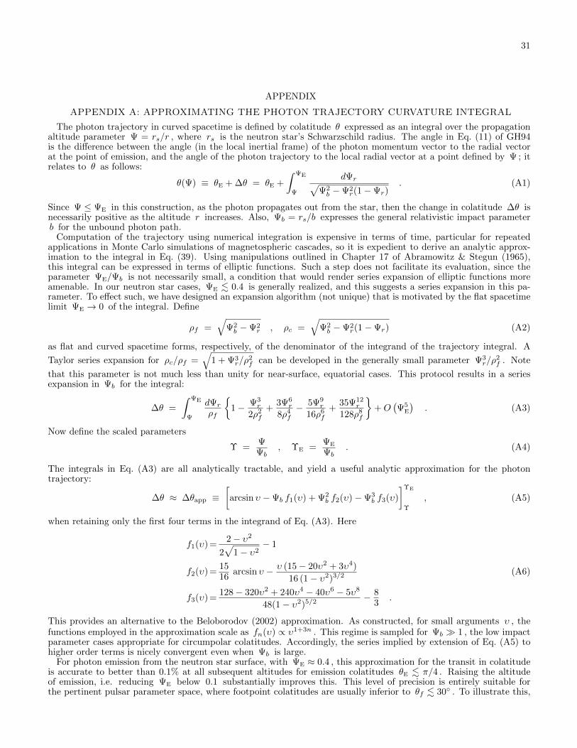
31

APPENDIX

APPENDIX A: APPROXIMATING THE PHOTON TRAJECTORY CURVATURE INTEGRAL

The photon trajectory in curved spacetime is defined by colatitude θ expressed as an integral over the propagationaltitude parameter Ψ = rs/r , where rs is the neutron star’s Schwarzschild radius. The angle in Eq. (11) of GH94is the difference between the angle (in the local inertial frame) of the photon momentum vector to the radial vectorat the point of emission, and the angle of the photon trajectory to the local radial vector at a point defined by Ψ ; itrelates to θ as follows:

θ(Ψ) ≡ θE + ∆θ = θE +

∫ ΨE

Ψ

dΨr√Ψ2b −Ψ2

r(1−Ψr). (A1)

Since Ψ ≤ ΨE in this construction, as the photon propagates out from the star, then the change in colatitude ∆θ isnecessarily positive as the altitude r increases. Also, Ψb = rs/b expresses the general relativistic impact parameterb for the unbound photon path.

Computation of the trajectory using numerical integration is expensive in terms of time, particular for repeatedapplications in Monte Carlo simulations of magnetospheric cascades, so it is expedient to derive an analytic approx-imation to the integral in Eq. (39). Using manipulations outlined in Chapter 17 of Abramowitz & Stegun (1965),this integral can be expressed in terms of elliptic functions. Such a step does not facilitate its evaluation, since theparameter ΨE/Ψb is not necessarily small, a condition that would render series expansion of elliptic functions moreamenable. In our neutron star cases, ΨE . 0.4 is generally realized, and this suggests a series expansion in this pa-rameter. To effect such, we have designed an expansion algorithm (not unique) that is motivated by the flat spacetimelimit ΨE → 0 of the integral. Define

ρf =√

Ψ2b −Ψ2

r , ρc =√

Ψ2b −Ψ2

r(1−Ψr) (A2)

as flat and curved spacetime forms, respectively, of the denominator of the integrand of the trajectory integral. A

Taylor series expansion for ρc/ρf =√

1 + Ψ3r/ρ

2f can be developed in the generally small parameter Ψ3

r/ρ2f . Note

that this parameter is not much less than unity for near-surface, equatorial cases. This protocol results in a seriesexpansion in Ψb for the integral:

∆θ =

∫ ΨE

Ψ

dΨr

ρf

1− Ψ3

r

2ρ2f

+3Ψ6

r

8ρ4f

− 5Ψ9r

16ρ6f

+35Ψ12

r

128ρ8f

+O

(Ψ5

E

). (A3)

Now define the scaled parameters

Υ =ΨΨb

, ΥE =ΨE

Ψb. (A4)

The integrals in Eq. (A3) are all analytically tractable, and yield a useful analytic approximation for the photontrajectory:

∆θ ≈ ∆θapp ≡[arcsin υ −Ψb f1(υ) + Ψ2

b f2(υ)−Ψ3b f3(υ)

]ΥE

Υ

, (A5)

when retaining only the first four terms in the integrand of Eq. (A3). Here

f1(υ) =2− υ2

2√

1− υ2− 1

f2(υ) =1516

arcsin υ − υ (15− 20υ2 + 3υ4)

16 (1− υ2)3/2 (A6)

f3(υ) =128− 320υ2 + 240υ4 − 40υ6 − 5υ8

48(1− υ2)5/2 − 83

.

This provides an alternative to the Beloborodov (2002) approximation. As constructed, for small arguments υ , thefunctions employed in the approximation scale as fn(υ) ∝ υ1+3n . This regime is sampled for Ψb 1 , the low impactparameter cases appropriate for circumpolar colatitudes. Accordingly, the series implied by extension of Eq. (A5) tohigher order terms is nicely convergent even when Ψb is large.

For photon emission from the neutron star surface, with ΨE ≈ 0.4 , this approximation for the transit in colatitudeis accurate to better than 0.1% at all subsequent altitudes for emission colatitudes θE . π/4 . Raising the altitudeof emission, i.e. reducing ΨE below 0.1 substantially improves this. This level of precision is entirely suitable forthe pertinent pulsar parameter space, where footpoint colatitudes are usually inferior to θf . 30 . To illustrate this,

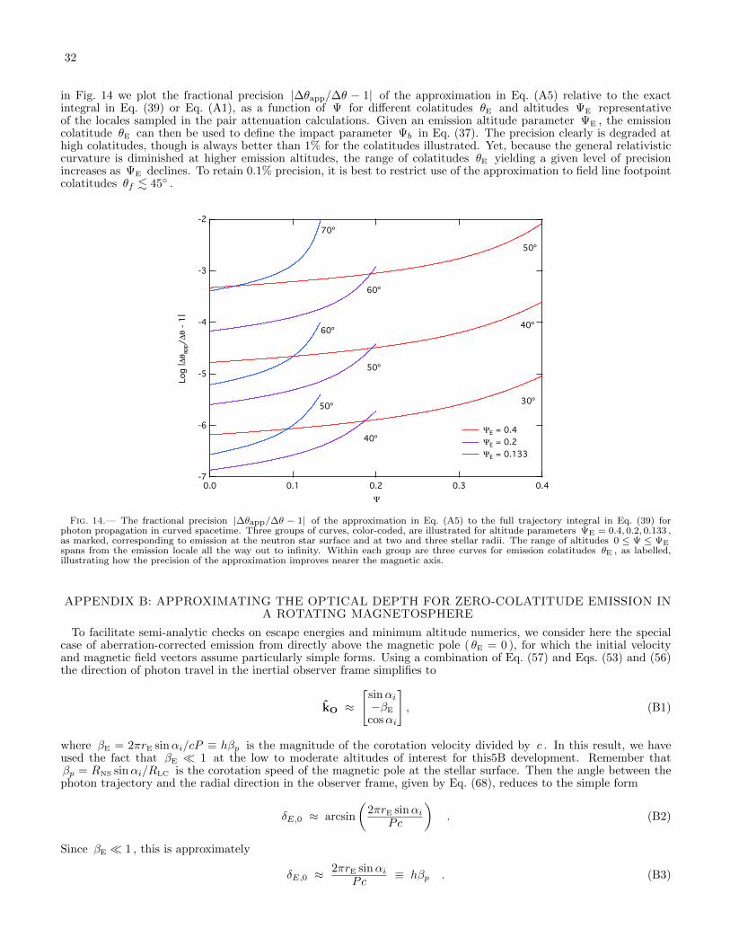
32

in Fig. 14 we plot the fractional precision |∆θapp/∆θ − 1| of the approximation in Eq. (A5) relative to the exactintegral in Eq. (39) or Eq. (A1), as a function of Ψ for different colatitudes θE and altitudes ΨE representativeof the locales sampled in the pair attenuation calculations. Given an emission altitude parameter ΨE , the emissioncolatitude θE can then be used to define the impact parameter Ψb in Eq. (37). The precision clearly is degraded athigh colatitudes, though is always better than 1% for the colatitudes illustrated. Yet, because the general relativisticcurvature is diminished at higher emission altitudes, the range of colatitudes θE yielding a given level of precisionincreases as ΨE declines. To retain 0.1% precision, it is best to restrict use of the approximation to field line footpointcolatitudes θf . 45 .

-7

-6

-5

-4

-3

-2

Log |

∆θ

app/

∆θ -

1|

0.40.30.20.10.0

Ψ

50¼

70¼

30¼

60¼

40¼60¼

40¼

50¼

50¼

ΨE = 0.4

ΨE = 0.2

ΨE = 0.133

Fig. 14.— The fractional precision |∆θapp/∆θ − 1| of the approximation in Eq. (A5) to the full trajectory integral in Eq. (39) forphoton propagation in curved spacetime. Three groups of curves, color-coded, are illustrated for altitude parameters ΨE = 0.4, 0.2, 0.133 ,as marked, corresponding to emission at the neutron star surface and at two and three stellar radii. The range of altitudes 0 ≤ Ψ ≤ ΨEspans from the emission locale all the way out to infinity. Within each group are three curves for emission colatitudes θE , as labelled,illustrating how the precision of the approximation improves nearer the magnetic axis.

APPENDIX B: APPROXIMATING THE OPTICAL DEPTH FOR ZERO-COLATITUDE EMISSION INA ROTATING MAGNETOSPHERE

To facilitate semi-analytic checks on escape energies and minimum altitude numerics, we consider here the specialcase of aberration-corrected emission from directly above the magnetic pole ( θE = 0 ), for which the initial velocityand magnetic field vectors assume particularly simple forms. Using a combination of Eq. (57) and Eqs. (53) and (56)the direction of photon travel in the inertial observer frame simplifies to

kO ≈

[sinαi−βE

cosαi

], (B1)

where βE = 2πrE sinαi/cP ≡ hβp is the magnitude of the corotation velocity divided by c . In this result, we haveused the fact that βE 1 at the low to moderate altitudes of interest for this5B development. Remember thatβp = RNS sinαi/RLC is the corotation speed of the magnetic pole at the stellar surface. Then the angle between thephoton trajectory and the radial direction in the observer frame, given by Eq. (68), reduces to the simple form

δE,0 ≈ arcsin

(2πrE sinαi

Pc

). (B2)

Since βE 1 , this is approximately

δE,0 ≈2πrE sinαi

Pc≡ hβp . (B3)

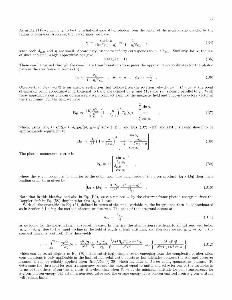
33

As in Eq. (11) we define χ to be the radial distance of the photon from the center of the neutron star divided by theradius of emission. Applying the law of sines, we have

χ =sin δE,0

sin(δE,0 − η)≈ 1

1− η/δE,0, (B4)

since both δE,0 and η are small. Accordingly, escape to infinity corresponds to η → δE,0 . Similarly, for s , the lawof sines and small-angle approximations give

s ≈ rE (χ− 1) . (B5)

These can be carried through the coordinate transformations to express the approximate coordinates for the photonpath in the star frame in terms of η :

rS ≈rE

1− η/δE,0, θS ≈ η , φS ≈ −

π2

. (B6)

Observe that φS ≈ −π/2 is an angular restriction that follows from the rotation velocity ~βE = Ω × rE at the pointof emission being approximately orthogonal to the plane defined by ~µ and Ω , since rE is nearly parallel to ~µ . Withthese approximations one can obtain a relatively compact form for the magnetic field and photon trajectory vector inthe star frame. For the field we have

BS ≈3BpR

3NS

2r3E

(1− η

δE,0

)3

TΩ(tO) ·

23

sinαi

−η23

cosαi

, (B7)

which, using ΩtO ≈ s/RLC ≈ δE,0η/[(δE,0 − η) sinαi] 1 and Eqs. (B2), (B3) and (B4), is easily shown to beapproximately equivalent to

BS ≈Bph3

(1− η

δE,0

)3

sinαi

−32η +

δE,0ηδE,0 − η

cosαi

, (B8)

The photon momentum vector is

kS ≈ ω

sinαiδE,0ηδE,0 − ηcosαi

, (B9)

where the y component is far inferior to the other two. The magnitude of the cross product |kS × BS| then has aleading order term given by ∣∣∣kS ×BS

∣∣∣ ≈ 3ωBp2h3

η (δE,0 − η)3

δ3E,0

. (B10)

Note that in this identity, and also in Eq. (B9), we can replace ω by the observer frame photon energy ε since theDoppler shift in Eq. (58) simplifies for this βE 1 case.

With all the quantities in Eq. (51) defined in terms of the small variable η , the integral can then be approximatedas in Section 3.1 using the method of steepest descents. The peak of the integrand occurs at

ηpk =δE,0

4, (B11)

as we found for the non-rotating, flat spacetime case. In practice, the attenuation rate drops to almost zero well belowηmax ≈ δE,0 , due to the rapid decline in the field strength at high altitudes, and therefore we set ηmax → ∞ in thesteepest descents protocol. This then yields

τ =

∫ ηmax

0

Rds

dηdη ≈ 36

√3

218αfλ–BpR

3NS

r2E

√8π4BpR3

NSε sin3 αic3P 3

exp

− 211cPr2

E

35εBpπR3 sinαi

, (B12)

which can be recast slightly as Eq. (70). This satisfyingly simple result emerging from the complexity of aberrationconsiderations is only applicable in the limit of non-relativistic boosts at low altitudes between the star and observerframes: it can be reliably applied when RLC/RNS & 30 , which includes all Fermi young gamma-ray pulsars. Todetermine the threshold for pair transparency, we set this integral equal to unity, and solve for one of the variables interms of the others. From this analysis, it is clear that when θE → 0 , the minimum altitude for pair transparency fora given photon energy will attain a non-zero value and the escape energy for a photon emitted from a given altitudewill remain finite.

34