Sampling bias and logistic models - University of Chicagopmcc/reports/bias.pdf · ·...
35
© 2008 Royal Statistical Society 1369–7412/08/70643 J. R. Statist. Soc. B (2008) 70, Part 4, pp. 643–677 Sampling bias and logistic models Peter McCullagh University of Chicago, USA [Read before The Royal Statistical Society at a meeting organized by the Research Section on Wednesday , February 6th, 2008 , Professor I. L. Dryden in the Chair ] Summary. In a regression model, the joint distribution for each finite sample of units is deter- mined by a function p x .y/ depending only on the list of covariate values x D .x.u 1 /,...,x.u n // on the sampled units. No random sampling of units is involved. In biological work, random sampling is frequently unavoidable, in which case the joint distribution p.y, x/ depends on the sampling scheme. Regression models can be used for the study of dependence provided that the conditional distribution p.yjx/ for random samples agrees with p x .y/ as determined by the regression model for a fixed sample having a non-random configuration x. The paper develops a model that avoids the concept of a fixed population of units, thereby forcing the sampling plan to be incorporated into the sampling distribution. For a quota sample having a predetermined covariate configuration x, the sampling distribution agrees with the standard logistic regres- sion model with correlated components. For most natural sampling plans such as sequential or simple random sampling, the conditional distribution p.yjx/ is not the same as the regression distribution unless p x .y/ has independent components. In this sense, most natural sampling schemes involving binary random-effects models are biased.The implications of this formulation for subject-specific and population-averaged procedures are explored. Keywords: Autogenerated unit; Correlated binary data; Cox process; Estimating function; Interference; Marginal parameterization; Partition model; Permanent polynomial; Point process; Prognostic distribution; Quota sample; Random-effects model; Randomization; Self-selection; Size-biased sample; Stratum distribution 1. Introduction Regression models are the primary statistical tool for studying the dependence of a response Y on covariates x in a population U . For each finite sample of units or subjects u 1 ,..., u n , a regres- sion model specifies the joint distribution p x .y/ of the response y = .Y.u 1 /,..., Y.u n // on the given units. Implicit in the notation is the exchangeability assumption, that two samples having the same list of covariate values have the same joint distribution p x .y/. All generalized linear models have this property, and many correlated Gaussian models have the same property, e.g. p x .A/ = N n .Xβ, σ 2 0 I n + σ 2 1 K[x]/.A/, .1/ where N n .μ, Σ/.A/ is the probability assigned by the n-dimensional Gaussian distribution to the event A ⊂ R n . The mean μ = Xβ is determined by the covariate matrix X , and K ij [x] = K{x.u i /, x.u j /} is a covariance function evaluated at the points x. Depending on the area of application, it may happen that the target population is either unlabelled, or random in the sense that the units are generated by the process as it evolves. Con- sider, for example, the problem of estimating the distribution of fibre lengths from a specimen of woollen or cotton yarn, or the problem of estimating the distribution of speeds of highway Address for correspondence: Peter McCullagh, Department of Statistics, University of Chicago, 5734 Univer- sity Avenue, Chicago, IL 60657-1514, USA. E-mail: [email protected]
Transcript of Sampling bias and logistic models - University of Chicagopmcc/reports/bias.pdf · ·...
© 2008 Royal Statistical Society 1369–7412/08/70643
J. R. Statist. Soc. B (2008)70, Part 4, pp. 643–677
Sampling bias and logistic models
Peter McCullagh
University of Chicago, USA
[Read before The Royal Statistical Society at a meeting organized by the Research Section onWednesday , February 6th, 2008, Professor I. L. Dryden in the Chair ]
Summary. In a regression model, the joint distribution for each finite sample of units is deter-mined by a function px.y/ depending only on the list of covariate values x D .x.u1/,. . .,x.un//on the sampled units. No random sampling of units is involved. In biological work, randomsampling is frequently unavoidable, in which case the joint distribution p.y, x/ depends on thesampling scheme. Regression models can be used for the study of dependence provided thatthe conditional distribution p.yjx/ for random samples agrees with px.y/ as determined by theregression model for a fixed sample having a non-random configuration x. The paper developsa model that avoids the concept of a fixed population of units, thereby forcing the sampling planto be incorporated into the sampling distribution. For a quota sample having a predeterminedcovariate configuration x, the sampling distribution agrees with the standard logistic regres-sion model with correlated components. For most natural sampling plans such as sequential orsimple random sampling, the conditional distribution p.yjx/ is not the same as the regressiondistribution unless px.y/ has independent components. In this sense, most natural samplingschemes involving binary random-effects models are biased.The implications of this formulationfor subject-specific and population-averaged procedures are explored.
Keywords: Autogenerated unit; Correlated binary data; Cox process; Estimating function;Interference; Marginal parameterization; Partition model; Permanent polynomial; Pointprocess; Prognostic distribution; Quota sample; Random-effects model; Randomization;Self-selection; Size-biased sample; Stratum distribution
1. Introduction
Regression models are the primary statistical tool for studying the dependence of a response Yon covariates x in a population U . For each finite sample of units or subjects u1, . . . , un, a regres-sion model specifies the joint distribution px.y/ of the response y = .Y.u1/, . . . , Y.un// on thegiven units. Implicit in the notation is the exchangeability assumption, that two samples havingthe same list of covariate values have the same joint distribution px.y/. All generalized linearmodels have this property, and many correlated Gaussian models have the same property, e.g.
px.A/=Nn.Xβ,σ20In +σ2
1 K[x]/.A/, .1/
where Nn.μ, Σ/.A/ is the probability assigned by the n-dimensional Gaussian distribution tothe event A ⊂ Rn. The mean μ= Xβ is determined by the covariate matrix X , and Kij[x] =K{x.ui/, x.uj/} is a covariance function evaluated at the points x.
Depending on the area of application, it may happen that the target population is eitherunlabelled, or random in the sense that the units are generated by the process as it evolves. Con-sider, for example, the problem of estimating the distribution of fibre lengths from a specimenof woollen or cotton yarn, or the problem of estimating the distribution of speeds of highway
Address for correspondence: Peter McCullagh, Department of Statistics, University of Chicago, 5734 Univer-sity Avenue, Chicago, IL 60657-1514, USA.E-mail: [email protected]
644 P. McCullagh
vehicles. Individual fibres are clearly unlabelled, so it is necessary to select a random sample,which might be size biased. Highway vehicles may be labelled by registration number, but thetarget population is weighted by frequency or intensity of highway use, so the units (travellingvehicles) are generated by the process itself. In many areas of application, the set of units evolvesrandomly in time, e.g. human or animal populations. The concept of a fixed subset makes littlesense physically or mathematically, so random samples are inevitable. The sample might beobtained on the fly by sequential recruitment in a clinical trial, or by recording passing vehi-cles at a fixed point on the highway, or it might be obtained by simple random sampling, orby a more complicated ascertainment scheme in studies of genetic diseases. The observationfrom such a sample is a random variable, possibly bivariate, whose distribution depends on thesampling protocol. In the application of regression models, it is often assumed that the jointdistribution p.x, y/ is such that the conditional distribution p.y|x/ is the same as the distributionpx.y/ determined by the regression model for a sample having a predetermined covariate confi-guration. The main purpose of this paper is to reconsider this assumption in the context of binaryand polytomous regression models that incorporate random effects or correlation betweenunits.
2. Binary regression models
The conventional, most direct, and apparently most natural way to incorporate correlation intoa binary response model is to include additive random effects on the logistic scale (Laird andWare, 1982; McCullagh and Nelder, 1989; Breslow and Clayton, 1993; McCulloch, 1994, 1997;Lee et al., 2006). The random effects in a hierarchical model need not be Gaussian, but a gen-eralized linear mixed model of that type with a binary response Y and a real-valued covariate xsuffices to illustrate the idea. The first step is to construct a Gaussian process η on R with zeromean and covariance function K. For example, we might have K.x, x′/ =σ2 exp.−|x − x′|=τ /,so that η is a continuous random function. Alternatively, K could be a block factor expressedas a Boolean matrix, so that η is constant on blocks or clusters, with block effects that areindependent and identically distributed. Given η, the components of Y are independent andare such that
logit[pr{Y.u/=1|η}]=α+β x.u/+η{x.u/}, .2/
where Y.u/ is the response and x.u/ the covariate value on unit u. As a consequence, two unitshaving the same or similar covariate values have identical or similar random contributionsη{x.u/} and η{x.u′/}, and the responses Y.u/ and Y.u′/ are positively correlated. Since η isa random variable, the joint density at y = .y1, . . . , yn/ for any fixed sample of n units havingcovariate values x = .x1, . . . , xn/ is
px.y/=∫
Rn
n∏j=1
exp{.α+βxj +ηj/yj}1+ exp.α+βxj +ηj/
φ.η; K/dη: .3/
The word model refers to these distributions, not to the random variable (2). In this instancewe obtain a four-parameter regression model with parameters .α,β,σ, τ /.
The simplest polytomous version of model (3) requires k correlated processes, η0.x/, . . . ,ηk−1.x/, one for each class. The joint probability distribution
px.y/=∫
Rnk
n∏j=1
exp{αyj +βyj xj +ηyj .xj/}k−1∑
0exp{αr +βrxj +ηr.xj/}
φ.η; K/dη .4/
Sampling Bias and Logistic Models 645
depends only on the distribution of differences ηr.x/−η0.x/. Setting α0 =β0 =η0.x/=0 intro-duces the asymmetry in model (3), but no loss of generality. In the econometrics literature,model (4) is known as a discrete choice model with random effects, and C ={0, . . . , k −1} is theset of mutually exclusive choices or brand preferences, which is seldom exhaustive.
The term regression model used in connection with distributions (1), (3) and (4) does not implyindependence of components, but it does imply lack of interference in the sense that the covari-ate value x′ =x.u′/ on one unit has no effect on the response distribution for other units (Cox(1958), section 2.4, and McCullagh (2005)). The mathematical definition for a binary model is
px,x′.y, 0/+px,x′.y, 1/=px.y/, .5/
which is satisfied by model (3) regardless of the distribution of η. Here px,x′.·/ is the responsedistribution for a set of n + 1 units, the first n of which have covariate vector x. For furtherdiscussion, see Sections 6 and 8.1.
In any extension of a regression model to a bivariate process, two possible interpretations maybe given to the functions px.y/. Given x = .x1, . . . , xn/, the stratum distribution is the marginaldistribution of Y.u1/, . . . , Y.un/ for a random set of units selected so that x.ui/=xi. Ordinarily,this is different from the conditional distribution pn.y|x/ for a fixed set of n units having arandom configuration x. Stratum distributions automatically satisfy the no-interference prop-erty, so the most natural extension uses px.y/ for stratum distributions, as in Section 3. In theconventional hierarchical extension, the two distributions are equal, and the regression modelpx.y/ serves both purposes.
The distinction between conditional distribution and stratum distribution is critical in muchof what follows. If the units were generated by a random process or selected by random sam-pling, then x would indeed be a random variable whose distribution depends on the samplingplan. In a marketing study, for example, it is usual to focus on the subset of consumers whoactually purchase one of the study brands, in which case the sample units are generated by theprocess itself. Participants in a clinical trial are volunteers who satisfy the eligibility criteria andgive informed consent. The study units are not predetermined but are generated by a randomprocess. Such units, whether they be patients, highway vehicles or purchase events, are calledautogenerated ; the non-mathematical term self-selected is too anthropocentric for general use.Without careful verification, we should not expect the conditional distribution pn.y|x/ forautogenerated units to coincide with px.y/ for a predetermined configuration x. We could, ofcourse, extend the regression model (4) to an exchangeable bivariate process by asserting thatthe components of x are independent and identically distributed with px.y/ as the conditionaldistribution. This extension guarantees pn.y|x/=px.y/ by fiat, which is conventional but notnecessarily natural. It does not address the critical modelling problem, that labels are usuallyaffixed to the units after they have been generated by the process itself.
In principle, the parameters in models (3) or (4) can be estimated in the standard way by usingthe marginal likelihood function, either by maximization or by using a formal Bayesian modelwith a prior distribution on .α,β,σ, τ /. Alternatively, it may be possible for some purposesto avoid integration by using a Laplace approximation or penalized likelihood function alongthe lines of Schall (1991), Breslow and Clayton (1993), Wolfinger (1993), Green and Silverman(1994) or Lee and Nelder (1996).
The binary model (3) and the polytomous version (4) are satisfactory in many ways, but theysuffer from at least four defects as follows.
(a) Parameter attenuation: suppose that x = .z, x′/ has several components, one of whichis the treatment status, and that βx is a linear combination. The odds of success
646 P. McCullagh
are p.1,x′/.1/=p.1,x′/.0/ for a treated unit having baseline covariate value x′, andp.0,x′/.1/=p.0,x′/.0/ for an untreated unit, and the treatment effect is the ratio of thesenumbers. In ordinary linear logistic models with independent components, the coeffi-cient of treatment status is the treatment effect on the log-scale. However, the treatmenteffect in model (3) is a complicated function of all parameters. In itself, this is not a seriousdrawback, but it does complicate inferential statements about the principal target param-eter if model (3) is taken seriously.
(b) Class aggregation: suppose that two response classes r and s in model (4) are such thatαr =αs, βr =βs and .ηr, ηs/∼ .ηs, ηr/ have the same distribution. Although these classesare homogeneous, the marginal distribution after aggregation of classes is not of thesame form. In other words, the binary model (3) cannot be obtained from (4) by aggre-gation of homogeneous classes.
(c) Class restriction: suppose that the number of classes in model (4) is initially large, but wechoose to focus on a subset, ignoring the remainder. In a study of causes of death, forexample, we might focus on cancer deaths, ignoring deaths due to other causes. Patientsdying of cancer constitute a random subset of all deaths, so the x-values and y-valuesare both random, with distribution determined implicitly by model (4). On this randomsubset, the conditional distribution of y given x does not have the form (4). In parti-cular, the binary model (3) cannot be obtained from (4) by restriction of responseclasses.
(d) Sampling distributions: if the sampling procedure is such that the number of sampledunits or configuration of x-values is random, the conditional distribution of the responseon the sampled units pn.y|x/ may be different from model (3).
Parameter attenuation is not, in itself, a serious defect. The real defect lies in the fact that, formany natural sampling protocols, parameter attenuation is a statistical artefact stemming frominappropriate model assumptions. The illusion of attenuation is attributable to sampling bias,the fact that the sample units are not predetermined but are generated by a random process thatthe conventional hierarchical model is incapable of taking into account. The distinction that isfrequently drawn between subject-specific effects and population-averaged effects (Zeger et al.,1988; Galbraith, 1991) is a manifestation of the same phenomenon (Section 8.2).
3. An evolving population model
3.1. The processLet X be the covariate space, and let ν be a measure in X such that ν is finite and positive onnon-empty open sets. In other words 0 < ν.X / < ∞, and ν.dx/ = ν.dx/=ν.X / is a probabilitydistribution on X with positive density at each point. In addition, C = {0, . . . , k − 1} is the setof response classes, and λ.r, x/ is the value at .r, x/ of a random intensity function on C ×X ,positive and bounded. For notational convenience we write λr.x/ for λ.r, x/ and λ•.x/=Σλr.x/
for the total intensity at x. A Poisson process in C ×X × .0, ∞/ evolves at a constant temporalrate λ.r, x/ν.dx/dt. These events constitute the target population, which is random, infinite andunlabelled.
Let Zt be the set of events occurring before time t, and Z=Z∞. Each point in Z is an orderedtriple z= .y, x, t/ where x.z/ is the spatial co-ordinate, t.z/ is the temporal co-ordinate and y.z/ isthe class. Given λ, the number of events in Zt is Poisson with mean t
∫X λ•.x/ν.dx/, proportional
to t and finite. The number of events in Z is infinite, and the set of points {x.z/ : z∈Z} is densein X .

Sampling Bias and Logistic Models 647
The Cox process provides a complete description of the random subset Z⊂C ×X × .0, ∞/.Since Z is a random set, there can be no concept of a fixed subset or sample in the conventionalsense. Nonetheless, the distribution of Z is well defined, so it is possible to compute the distribu-tion for the observation generated by a well-specified sampling plan. It is convenient for manypurposes to take U ={1, 2, . . .} to be the set of natural numbers, and to order the elements of Ztemporally, so that tj = t.j/ is the time of occurrence of the jth event, x.j/ is the spatial co-ordi-nate and y.j/ is the type or class. The ordered event times 0≡ t0 � t1 � t2 � · · · are distinct withprobability 1. With this convention, the sequence .xj, yj, tj − tj−1/ is infinitely exchangeable.The components are conditionally independent given λ, and identically distributed with jointdensity
E
[Λ• exp{−Λ•.tj − tj−1/}dtj
λ•.xj/ν.dxj/
Λ•
λyj .xj/
λ•.xj/
]
averaged over the intensity functionλ. The total intensity Λ• =∫λ•.x/ν.dx/ is the rate of accrual,
which is random but constant in time.
3.2. Sampling protocolsSix sampling protocols are considered, some being more natural than others because they canbe implemented in finite time. The first is a quota sample with covariate configuration x as thetarget. The second is a sequential sample consisting of the first n events and the third is the setZt for fixed t. The fourth is a simple random sample from Zt at some suitably large time. Thefinal protocol is a retrospective or case–control sample in which the number of successes andfailures is predetermined.
3.2.1. Quota sampleLet x = .x1, . . . , xn/ be a given ordered set of n points in X , and let dxj be an open intervalcontaining xj. For convenience of exposition, it is assumed that the points are distinct and theintervals disjoint. A sample from U is an ordered list of distinct elements ϕ1, . . . ,ϕn, and thequota is satisfied if x.ϕj/∈dxj. The easiest way to select such a sample is to partition the pop-ulation by covariate values Zdx ={.x, y, t/∈Z : x∈dx}. Each stratum is infinite and temporallyordered. Define ϕj to be the index of the first event in Zdxj
.Distributions are computed for the limit in which each interval dxj tends to a point, so the
distribution of the spatial component is degenerate at x. The temporal component t.ϕj/ is condi-tionally exponential with parameter Λ•.dxj/, so t.ϕj/→∞. The distribution of the class labels is
pn.y|x/=E
{n∏
i=1
λyi .xi/
λ•.xi/
}: .6/
The conditional distribution is independent of ν and coincides with px.y/ in model (4) whenwe set
log{λr.x/}=αr +βrx+ηr.x/:
In other words, the Cox process is fully compatible with the standard logistic model (3) or (4),and quota sampling is unbiased in the sense that the conditional distribution pn.y|x/ coincideswith px.y/ in model (4).
3.2.2. Sequential sampleLet n be given, and let the sample ϕ consist of the first n events in temporal order. Given theintensity function, the temporal component of the events is a homogeneous Poisson process
648 P. McCullagh
with rate Λ• =∫λ•.x/ν.dx/. The conditional joint density of the sampled time points is thus
Λn• exp.−Λ•tn/ for 0 � t1 � · · ·� tn. The components of xϕ are conditionally independent and
identically distributed with density λ•.x/ν.dx/=Λ•, and the components of yϕ are conditionallyindependent given xϕ=x with distribution
pr{y.ϕi/= r|x}=λr.xi/=λ•.xi/:
Given λ, the joint density of the sample values at .x, y, t/ is
pn.y, x, t|λ/dx dt =Λn• exp.−Λ•tn/
n∏i=1
λyi .xi/
λ•.xi/
λ•.xi/ν.dxi/
Λ•dti
= exp.−Λ•tn/∏λyi .xi/ν.dxi/dti,
so the unconditional joint density is
pn.y, x, t/dx dt =E
{exp.−Λ•tn/
n∏i=1
λyi .xi/ν.dxi/dti
}
averaged with respect to the distribution of λ.The joint density of .x, t/ is computed in the same way:
pn.x, t/dx dt =E
{exp.−Λ•tn/
n∏i=1
λ•.xi/ν.dxi/dti
}
so the conditional distribution of y given .x, t/ is
pn.y|x, t/=E
{exp.−Λ•tn/
n∏i=1
λyi .xi/
}
E
{exp.−Λ•tn/
n∏i=1
λ•.xj/
} : .7/
These calculations assume that event times are observed and recorded. Otherwise we need theconditional distribution of y given x, which is
pn.y|x/=E
{n∏
i=1λyi .xi/=Λ•
}
E
{n∏
i=1λ•.xi/=Λ•
} : .8/
In either case the conditional distribution is a ratio of expected values, whereas equation (6) isthe expected value of a ratio.
If the intensity ratio processes .λr.x/=λ0.x//x∈X are jointly independent of the total intensityprocess .λ•.x//x∈X , the conditional distribution pn.y|x/ coincides with model (4). Otherwise,sequential sampling is biased in the sense that p.y|x/ =px.y/.
3.2.3. Sequential sample for fixed timeIn this sampling plan the observation is the set Zt for fixed t. Given λ, the number of sampledevents n=#Zt is Poisson with parameter tΛ•. The probability of observing a specific sequenceof events and class labels is
pt.y, x, t/dx dt =E
{exp.−tΛ•/
n∏i=1
λyi .xi/ν.dxi/
}dt
Sampling Bias and Logistic Models 649
for n�0 and 0� t1 � · · ·� tn � t. Likewise, the marginal density of .x, t/ is
pt.x, t/dx dt =E
{exp.−tΛ•/
n∏i=1
λ•.xi/ν.dxi/
}dt
so the conditional distribution of y given .x, t/ for this protocol is
pt.y|x, t/=E
{exp.−tΛ•/
n∏i=1
λyi .xi/
}
E
{exp.−tΛ•/
n∏i=1
λ•.xi/
} : .9/
The conditional distribution depends on the observation period but is independent of the eventtimes t. Consequently pt.y|x/ coincides with equation (9).
3.2.4. Simple random sampleThe aim of simple random sampling is to select a subset uniformly at random among subsets ofa given size n. In the application at hand, the population is infinite, so simple random samplingis not well defined. However, a similar effect can be achieved by selecting N �n, and restrictingattention to the finite subset Zt ⊂ Z where t is the first time that #Zt �N. By exchangeability,the distribution of .y, x/ on a simple random sample is the same as the distribution on thefirst n events in temporal order. Apart from the temporal component, the sampling distribu-tions are the same as those in Section 3.2.2. Consequently, unless the intensity ratio processesare independent of λ•.·/, simple random sampling is biased.
3.2.5. Weighted sampleA weighted sample is one in which individual units are selected (thinned) with probability w.y, x/
depending on the response value. Examples with known weight functions arise in monetary unitsampling (Cox and Snell, 1979) and stereological sampling in mining applications (Baddeleyand Jensen, 2005). Restriction to a subset of C is an extreme special case in which w is zero oncertain classes and constant on the remainder. More generally, the self-selection of patients thatoccurs through informed consent in clinical trials may be modelled as an unknown weight func-tion. One way to generate such a sample is to observe the units as they arise in temporal order,retaining units independently with probability w.y, x/. This amounts to replacing the intensityfunction λ.y, x/ with the weighted version w.y, x/λ.y, x/. Weighted sampling is clearly biased.
3.2.6. Case–control sampleCase–control sampling is essentially the same as weighted sampling, except that k = 2 and thequota sizes n0 and n1 are predetermined. The sample for a case–control study consists of thefirst n0 events having y = 0 and the first n1 events having y = 1. Event times are not observed.An observation consists of a list x of n points in X together with a parallel list y of labels orclass types. The joint probability is
pn1n2.y, x/=E
{ ∏λyi .xi/ν.dxi/
Λ0.X /n0 Λ1.X /n1
},
and the conditional probability given x is proportional to
pn1n2.y|x/∝E
{ ∏λyi .xi/
Λ0.X /n0 Λ1.X /n1
}:
650 P. McCullagh
The approximation derived in Section 4 is equivalent to assuming that, for some measure ν, therandom normalized function λ0.x/=Λ0.X / is independent of the integral Λ0 = ∫
λ0.x/ν.dx/,and likewise for λ1. Using this approximation, the conditional probability is proportional to
pn1n2.y|x/∝E
{n∏
i=1λyi .xi/
}:
In essence, this means that the observation from a case–control design can be analysed as if itwere obtained from a prospective sequential sample or simple random sample as in Sections3.2.2–3.2.4.
3.3. Exchangeable sequences and conditional distributionsThe sequence .y1, x1/, .y2, x2/, . . . generated in temporal order by the evolving population modelis exchangeable. In contexts such as this, two interpretations of conditional probability andconditional expectation are prevalent in applied work. The probabilistic interpretation is notso much an interpretation as a definition; pr.yu = y|xu = x/ = p1.y, x/=p1.x/ as computed inequation (8) for n = 1. Here, u is fixed, xu is random and we select from the family of condi-tional distributions the one corresponding to the event xu =x. The stratum interpretation refersto the marginal distribution of the random variable y.uÅ/, where uÅ is the first element forwhich xuÅ = x. Here, uÅ is random, xuÅ is fixed and px.y/ is the marginal distribution of eachcomponent in stratum x as defined in equations (6) or (4) for n=1.
In an exchangeable bivariate process, each finite dimensional joint distribution factorspn.y, x/=pn.x/pn.y|x/. If the conditional distributions satisfy the ‘no-interference’ condition(5), the stratum distributions coincide with the conditional distributions, the conditional dis-tributions determine a regression model and the bivariate process is called conventional or hier-archical. Otherwise, if the conditional distributions do not determine a regression model, thestratum distributions are not the same as the conditional distributions. The risk in applied workis that the marginal mean μ.x/=∫
y px.dy/ in stratum x might be mistaken for the conditionalmean κ.x/=∫
y p.dy|x/.The notation E.yu|xu = x/ is widely used and dangerously ambiguous. The preferred inter-
pretation has the index u fixed and xu random, so E.y7|x7 =3/=κ.3/ is a legitimate expression.In biostatistical work on random-effects models, the stratum interpretation with fixed x andrandom u is predominant. This interpretation is not unreasonable if properly understood andconsistently applied, but it would be less ambiguous if written in the formμ.x/=E.yu|u: xu =x/.The longer version makes it clear that
E{y1 −μ.x1/|x1 =3}=κ.3/−μ.3/ =0,
with obvious implications for estimating equations (Section 7.1).The evolving population model shows clearly that the response distribution for a set of units
having a predetermined covariate configuration x is not necessarily the same as the conditionaldistribution for a simple random sample that happens to have the same covariate configura-tion. Thus, the sampling protocol cannot be ignored with impunity. For practical purposes, theplausible protocols are those that can be implemented in finite time, which implies sequentialsampling, weighted sampling or case–control sampling.
3.4. Variants and extensionsUp to this point, no assumptions have been made about the distribution ofλ. The evolving popu-lation model has two principal variants: one in which the k intensity functions λ0.·/, . . . ,λk−1.·/
Sampling Bias and Logistic Models 651
are independent, and the conventional one in which the total intensity process .λ•.x//x∈X isindependent of the intensity ratios .λr.x/=λ0.x//x∈X . The two types are not disjoint, but theintersection is small and relatively uninteresting. The characteristic property of the secondvariant is that the conditional sampling distribution for a sequential or simple random samplecoincides with the distribution px.y/ for predetermined x. Ambiguities concerning the samplingdistribution do not arise. Otherwise it is necessary to calculate the conditional distribution thatis appropriate for the sampling protocol. Each version of the evolving population model hasmerit. Both are closed under aggregation of classes because this amounts to replacing k by k −1and adding two of the intensity functions. Deletion or restriction of classes necessarily intro-duces a strong sampling bias. The total intensity is reduced so only the first variant is closedunder this operation. The Gaussian submodel (4) is not closed under aggregation of classes;nor is the log-Gaussian process that is described in Section 5.2.
In the evolving population model, the response on each unit is a point y.z/ in the finite setC. It is straightforward to modify this for a continuous response such as the speed of a vehiclepassing a fixed point on the highway. Counting measure in C must be replaced by a suitablefinite measure in the real line. To extend the model to a crossover design in which each unit isobserved twice, it is necessary to replace C by C2, or by .C ×{C, T}/2 for randomized treatment(Section 5.4). The random intensity function λ on .C × {C, T}/2 ×X governs the joint distri-bution of the x-values and the response–treatment pair at both time points. In a longitudinaldesign, observations on the same unit over time are understood to be correlated, and there mayalso be correlations between distinct units. To extend the model in this way, it is necessary toreplace C by a higher order product space, and to construct a suitable random intensity on thisspace. Such an extension is well beyond the scope of this paper.
4. Limit distributions
The conditional probability distribution
pt.y|x/=E
{exp .−Λ•t/
n∏i=1
λyi .xi/
}
E
{exp .−Λ•t/
n∏i=1
λ•.xi/
} = pt.y, x/
pt.x/.10/
in equations (7) and (9) is the ratio of the joint density and the marginal density. Ideally, theconditional distribution should be independent of the baseline measure, but this is not sobecause ν enters the definition of Λ• =
∫λ•.x/ν.dx/. However, this dependence is not very
strong, so it is reasonable to proceed by selecting a baseline measure that is both plausible andconvenient, rather than attempting to estimate ν. Plausible means that ν should be positive onopen sets.
The numerator and denominator both have non-degenerate limits as either t →0 for fixed ν,or the scalar ν.X /→0 for fixed t. The limiting low intensity conditional distribution
qn.y|x/=E
{n∏
i=1λyi .xi/
}
E
{n∏
i=1λ•.xi/
} .11/
is convenient for practical work because it is independent of ν. In addition, the product densitiesin the numerator and denominator are fairly easy to compute for a range of processes such as
652 P. McCullagh
log-Gaussian processes (Møller et al., 1998) and certain gamma processes (Shirai and Takahashi,2003; McCullagh and Møller, 2006). One can argue about the plausibility or relevance of thelimit, but the fact that the limit distribution is independent of ν is a definite plus.
The same limit distribution is obtained by a different sort of argument as follows. Supposethat there is a measure ν such that the nk ratios λ0.x/=Λ·, . . . ,λk−1.x/=Λ• for x ∈ x are jointlyindependent of Λ•. Then the numerator in equation (10) can be expressed as a product of expec-tations
E{exp.−tΛ•/∏λyi .xi/}=E{Λn
• exp.−tΛ•/}E
{λy1.x1/
Λ•· · · λyn.xn/
Λ•
}
= E{Λn• exp.−tΛ•/}E.Λn
• /E{∏
λyi .xi/}:
The denominator can be factored in a similar way, so the ratio in equation (10) simplifies toequation (11). If this condition is satisfied by ν, it is satisfied by all positive scalar multiples ofν, and the conditional distribution is unaffected.
The condition here is one of existence of a measure ν satisfying the independence condi-tion for the particular finite configuration x. In other words, the measure may depend on x,so the condition of existence is not especially demanding. Examples are given in McCullaghand Møller (2006) of intensity functions such that the ratios are independent of the integralwith respect to Lebesgue measure on a bounded subset of R or Rd . It is also possible to jus-tify the independence condition by a heuristic argument as follows. Suppose that λ.x/=T λ.x/
where λ is ergodic on R with unit mean, and T > 0 is distributed independently of λ. Then,if ν.dx/ = dx=2L for −L � x � L, we find that Λ• = T Λ• = T + o.1/ for large L, and the ratiosλ.x/=Λ• = λ.x/=Λ• are jointly independent of T by assumption. The independence assumptionis then satisfied in the limit as L→∞, and ν is, in effect, Lebesgue measure. For these reasons,the limit distribution (11) is used for certain calculations in the following section.
5. Two parametric models
5.1. Product densities and conditional distributionsAll the models in this section are such that λ0, . . . ,λk−1 are independent intensity functions. Theconditional distribution (11) is a distribution on partitions of x into k labelled classes, someof which might be empty. Denote by x.r/ the subset of x for which y = r. The numerator inequation (11) is the product
k−1∏r=0
E
{ ∏x∈x.r/
λ0.x/
}=m0.x.0// · · ·mk−1.x.k−1//
where mr is the product density for λr, and mr.∅/=1. The denominator is the product densityat x for the superposition process with intensity λ•. In other words, equation (11) is
qn.y|x/= m0.x.0// · · ·mk−1.x.k−1//
m•.x/, .12/
for partitions of x into k labelled classes. For prediction, the Papangelou conditional intensityis used. Suppose that .y, x/ has been observed in a sequential sample up to time t, and thatthe next subsequent event occurs at x′. The prognostic distribution for the response y′ is theconditional distribution given y, x and the value x′, which is
qn+1{y′ = r|.y, x, x′/}∝mr.x.r/ ∪{x′}/=mr.x.r//: .13/
Sampling Bias and Logistic Models 653
In general, the one-dimensional prognostic distribution is considerably easier to compute thanthe joint distribution.
The first task is to find product densities for specific parametric models.
5.2. Log-Gaussian modelLet log.λ/ be a Gaussian process in X with mean μ and covariance function K. In other words
E[log{λ.x/}]=μ.x/,
cov[log{λ.x/}, log{λ.x′/}]=K.x, x′/:
Then the expected value of the product m.x/=E{λ.x1/ · · ·λ.xn/} is
log{m.x/}= ∑x∈x
μ.x/+ 12
∑x,x′∈x
K.x, x′/:
This expression enables us to simplify the numerator in equation (11). Unfortunately, the sumof log-Gaussian processes is not log-Gaussian, so the normalizing constant is not available inclosed form. The logarithm of the conditional distribution (11) is given in an obvious notation by
log{qn.y|x/}= constant+∑μyi .xi/+ 1
2
k∑r=1
∑x,x′∈x.r/
Kr.x, x′/:
The prognostic distribution for a subsequent event at x′ is obtained from the product densityratios
qn+1{Y ′ = r|.y, x, x′/}∝ exp{μr.x′/+ 1
2 Kr.x′, x′/+ ∑
x∈x.r/
Kr.x, x′/}:
Without loss of generality, we may set μ0.x/ = 0. If the covariance functions are equal, theprognostic log-odds are
log-odds.Y ′ =1|. . ./=μ1.x′/+ ∑x∈x.1/
K.x, x′/− ∑x∈x.0/
K.x, x′/
for k=2. The conditional log-odds is a kernel function, an additive function of the sample valuesformally the same as Markov random-field models (Besag, 1974) except that the x-configurationis not predetermined or regular.
The log-Gaussian model with independent intensity functions is closed under restriction ofclasses. However, the sum of two independent log-Gaussian variables is not log-Gaussian, sothe model is not closed under aggregation of homogeneous classes. This remark applies also tothe model in Section 2. Failure of this property for homogeneous classes is a severe limitationfor practical work.
5.3. Gamma modelsLet Z1, . . . , Zd be independent zero-mean real Gaussian processes in X with covariance functionK /2, and let λ.x/ = Z2
1.x/ +· · ·+ Z2d.x/. Denote by K[x] the matrix with entries K.xi, xj/. For
any such matrix, the α-permanent is a weighted sum over permutations
perα.K[x]/=∑σα#σ
n∏i=1
K.xi, xσi /
where #σ is the number of cycles. The product density of λ at x is
E{λ.x1/ · · ·λ.xn/}=perd=2.K[x]/:
654 P. McCullagh
Under a certain positivity condition the process can be extended from the integers to all positivevalues of d. For a derivation of these results, see Shirai and Takahashi (2003) or McCullagh andMøller (2006).
In the homogeneous version of the gamma model, λr has product density perαr.K[x.r/]/, and
λ• has product density perα·.K[x]/. The conditional distribution (11) is
qn.y|x/= perα0.K[x.0/]/ · · ·perαk−1
.K[x.k−1/]/
perα·.K[x]/,
which is a generalization of the multinomial and Dirichlet–multinomial distributions. The prog-nostic distribution for a subsequent event at x′ is
qn+1.y′ = r|. . ./∝perαr.K[x.r/, x′]/=perαr
.K[x.r/]/:
By contrast with the log-Gaussian model, the prognostic log-odds is not a kernel function. Foran application of this model to classification, see McCullagh and Yang (2006).
The homogeneous gamma model can be extended in various ways, e.g. by replacingλr.x/ withexp.αr +βrx/λr.x/. Then the product density at x.r/ becomes exp.nrαr +βrx.r/
• / perαr.K[x.r/]/,
where nr =#x.r/ and x.r/• is the sum of the components. Alternatively, ifλr is replaced by τr λr.x/,
where τ0, . . . , τk−1 are independent scalars independent of λ, the product density is replaced byhr.nr/perαr
.K[x.r/]/ where hr.n/ is the nth moment of τr. Finally, there is a non-trivial limitdistribution as k →∞ and αr =α=k with α fixed (McCullagh and Yang, 2006).
5.4. Treatment effects and randomizationTo incorporate a non-random treatment effect, we replace C by C × {C, T}, where {C, T} arethe two treatment levels. Consider the binary model with multiplicative intensity function
λ.y, v, x/=λ.y, x/γ.y, v, x/ .14/
in which γ is a fixed parameter, and v is treatment status. Given λ, the treatment effect asmeasured by the conditional odds ratio is
τ .x/= γ.1, T , x/γ.0, C, x/
γ.0, T , x/γ.1, C, x/,
which is a non-random function of x, possibly a constant. Given an event z∈ Z with x.z/=x,the four possibilities for response and treatment status have probabilities proportional to
pr{y.z/=y, v.z/=v|z∈Z}∝E{λ.y, v, x/}=my.x/γ.y, v, x/:
Consequently the treatment effect as measured by the unconditional odds ratio is also τ .x/ withno attenuation. The stratum distribution px.·/ as defined in model (3) for fixed x gives a differentdefinition of treatment effect, one that is seldom relevant in applications.
For simplicity we now assume that the treatment effect is constant in x. The conditionaldistribution (11) for a sequential sample reduces to
qn.y, v|x/∝m0.x.0//m1.x.1//n∏
i=1γ.yi, vi/,
which is a bipartition model for response and treatment status. If m0 and m1 are known func-tions, this is the exponential family generated from (12) with canonical parameter log{γ.r, s/}
Sampling Bias and Logistic Models 655
and canonical statistic the array of counts in which nrs is the observed number of events forwhich y = r and v= s.
Suppose that .y, v, x/ has been observed in a sequential sample. The prognosis for the responsey′ for a subsequent event at x′ depends on whether v′ =T or v′ =C as follows:
odds.y′ =1|. . . , v′/= m1.x.1/, x′/m0.x.0//
m1.x.1//m0.x.0/, x′/γ.1, v′/γ.0, v′/
:
However, the prognostic odds ratio is equal to the treatment effect, again without attenuation.The preceding formulation of treatment effects is an attempt to incorporate into the sam-
pling model the notion that treatment status is the outcome of a random process. The modelwith constant treatment effect can be written in multiplicative form λ.y, x/γ.y, v/ as anintensity on C × {C, T} × X . The graphical representation with one node for each randomelement
shows that treatment status is conditionally independent of .λ, x/ given y. Although the conceptof treatment assignment is missing, the multiplicative intensity model describes accurately whatis achieved by randomization. The point process of events is such that treatment status v.z/ isconditionally independent of x.z/ given the response y.z/.
6. Interference
6.1. DefinitionLet px.·/ or p.·|x/ be a set of distributions defined for arbitrary finite configurations x. Lackof interference is a mathematical property ensuring that the n-dimensional distribution px.·/ isthe marginal distribution of the .n + 1/-dimensional distribution px,x′.·/ after integrating outthe last component. In symbols px.A/=px,x′.A×C/ for A⊂Cn, or
p.y ∈A|x/=p{.y, y′/∈A×C|.x, x′/}if applied to conditional distributions. When this condition is satisfied, the distribution of thefirst n components is unaffected by the covariate value for subsequent components. This is alsothe Kolmogorov consistency condition for a C-valued process in which the joint distribution ofY.u1/, . . . , Y.un/ depends on the covariate values x.u1/, . . . , x.un/ on those units. It is satisfiedby regression models such as (1), (3) and (4).
In the statistical literature on design, interference is usually understood in the physical orbiological sense, meaning carry-over effects from treatment applied to neighbouring plots. Fordetails and examples, see Cox (1958) or Besag and Kempton (1986). The definition does notdistinguish between physical interference and sampling interference, but this paper emphasizesthe latter.
To understand how sampling interference might arise, consider the simplest evolving popu-lation model in which X ={x} is a set containing a single point denoted by x. Let Y1, . . . be theclass labels in temporal order. Given λ, the number m of events in unit time is Poisson distributedwith parameter λ•, so m could be zero. However, given m, the values Y1, . . . , Ym are exchangeablewith one- and two-dimensional distributions
656 P. McCullagh
p1.Y1 = r|m�1/= E[{1− exp.−λ•/}λr=λ•]E{1− exp.−λ•/} E.λr/
E.λ•/,
p2.Y1 = r, Y2 = s|m�2/= E[{1− .1+λ•/ exp.−λ•/}λrλs=λ2• ]
E{1− .1+λ•/ exp.−λ•/} E.λrλs/
E.λ2• /
,
p2.Y1 = r|m�2/= E[{1− .1+λ•/ exp.−λ•/}λr=λ•]E{1− .1+λ•/ exp.−λ•/} E.λrλ•/
E.λ2• /
=p1.Y1 = r|m�1/:
In general, the probability assigned to the event Y1 = r by the bivariate distribution p2 is notthe same as the probability assigned to the same event by the one-dimensional distribution p1.The condition m� 2 in p2 implies an additional event at x, which may change the probabilitydistribution of Y1.
Two specific models are now considered: one exhibits interference; the other not. In the log-Gaussian model
log.λ0/∼N.μ0, 1/,
log.λ1/∼N.μ1, 1/
are independent random intensities. For a low intensity value .μ0,μ1/= .−5, − 4/, we find bynumerical integration that p1.Y1 = 0/ = 0:272 whereas p2.Y1 = 0/ = 0:201, so the interferenceeffect is substantial. The limiting low intensity approximations are 0.269 and 0.193 respectively.For .μ0,μ1/ = .−1, 0/ the mean intensities are .exp.−1
2 /, exp. 12 //, and the difference is less
marked: p1.Y1 =0/=0:310 versus p2.Y1 =0/=0:291.By contrast, consider the gamma model in which
λ0 ∼G.α0θ,α0/,
λ1 ∼G.α1θ,α1/
are independent with mean E.λr/=αrθ and variance αrθ2. The total intensity is distributed as
λ• ∼ G.α•θ,α•/ independently of the ratio, which has the beta distribution λ0=λ• ∼ B.α0,α1/.On account of independence, we find that p1.Y1 = 0/ = p2.Y1 = 0/ =α0=α•, so interference isabsent.
6.2. OverdispersionSuppose that events are grouped by covariate value, so that T•.x/ is the observed number ofevents at x, and Tr.x/ is the number of those who belong to class r. Overdispersion means thatthe variance of Tr.x/ exceeds the binomial variance, and the covariance matrix of T.x/ exceedsthe multinomial covariance. However, units having distinct x-values remain independent. Thiseffect is achieved by a Cox process driven by a completely independent random intensity takingindependent values at distinct points in X . Since units having distinct x-values remain indepen-dent, it suffices to describe the one-dimensional marginal distributions of the class totals at eachpoint in X .
Under the gamma model, the class totals at x are independent negative binomial randomvariables with means E.Tr/=γαr and variances γαr.1 +γ/. Given the total number of eventsat x, the conditional distribution is Dirichlet–multinomial
p.T = t|T• =m/= m!Γ.α•/
Γ.m+α•/
∏r∈C
Γ.tr +αr/
tr!Γ.αr/
Sampling Bias and Logistic Models 657
for non-negative tr such that t• = m. The sequence of values Y1, . . . , Ym is exchangeable, and,since there is no interference, the marginal distributions are independent of m:
pr.Y1 = r|m/=αr=α• =πr,
pr.Y1 = r, Y2 = s|m/=πrπs +{πr.1−πr/=.α• +1/ r = s,−πrπs=.α• +1/ otherwise.
Because of interference, no similar results exist for the log-Gaussian model.
7. Computation
7.1. Parameter estimationSince x and y are both generated by a random process, the likelihood function is determined bythe joint density. However, the joint distribution depends on the infinite dimensional nuisanceparameter ν.dx/, which governs primarily the marginal distribution of x. It appears that themarginal distribution of x must contain very little information about intensity ratios, so it isnatural to use the conditional distribution given x for inferential purposes. Likelihood calcula-tions using the exact conditional distribution (7)–(9) or the limit distributions (11) and (12) arecomplicated, though perhaps not impossible. We focus instead on parameter estimation usingunbiased estimating equations.
Let mr.x/ = E{λr.x/} be the mean intensity function for class r, m•.x/ the expected totalintensity at x, ρr.x/=E{λr.x/=λ•.x/} the expected value of the intensity ratio at x and πr.x/=mr.x/=m•.x/ the ratio of expected intensities. Sampling bias is the key to the distinction betweenρ.x/, the marginal distribution for fixed x, and π.x/, the conditional distribution for random xgenerated by a sequential sample from the process.
Consider a sequential sampling scheme in which the observation consists of the events Zt
for fixed t. The number of events #Zt , the values y.z/, x.z/ and π.x/ =π{x.z/} for z ∈ Zt areall random. It is best to regard Zt as a random measure in C × X whose mean has densityt my.x/ν.dx/ at .y, x/. The expected number of events in the interval dx is t m•.x/ν.dx/, andthe expected number of events of class r in the same interval is t mr.x/ν.dx/. For a functionh:X →R, additive functionals have expectation
E[∑
Zt
h{x.z/}]= t
∫X
h.x/m•.x/ν.dx/,
E[∑
Zt
h{x.z/}yr.z/]= t
∫X
h.x/mr.x/ν.dx/,
where y.z/ is the indicator function for the class, i.e. yr.z/=1 if the class is r. It follows that thesum Tr =ΣZ h.x/{yr.z/−πr.x/} has exactly zero mean for each function h. This first-momentcalculation involves only the first-order product densities. If it were necessary to calculate E.T |x/
given the configuration x, we should begin with the joint distribution or the conditional distri-bution (9). Because of interference, E.T |x/ is not 0; nor is E.T |#Zt/. Consequently, the momentcalculations in this section are fundamentally different from those of McCullagh (1983) or Zegerand Liang (1986).
The covariance of Tr and Ts is a sum of three terms: one associated with intrinsic Bernoullivariability, one with spatial correlation and one with interference. The expressions are simplifiedhere by setting h.x/=1.
658 P. McCullagh
cov.Tr, Ts/= t
∫X
{πr.x/δrs −πr.x/πs.x/}m•.x/ν.dx/
+ t2∫
X 2{πrs.x, x′/−πr•.x, x′/πs•.x
′, x/}m••.x, x′/ν.dx/ν.dx′/
+ t2∫
X 2Δr•.x, x′/Δs•.x
′, x/m••.x, x′/ν.dx/ν.dx′/: .15/
In these expressions, mrs.x, x′/ = E{λr.x/λs.x′/} is the second-order product density, and
πrs.x, x′/=mrs.x, x′/=m••.x, x′/ is the bivariate distribution for ordered pairs of distinct events.Roughly speaking, πr•.x, x′/ is the probability that the event at x is of class r given that an-other event occurs at x′. The difference Δr•.x, x′/ = πr•.x, x′/ − πr.x/, which is a measure ofsecond-order interference, is zero for conventional models. Both the gamma and the log-normal models exhibit interference, but the homogeneous gamma model has the special prop-erty of zero second-order interference.
The first integral in equation (15) can be consistently estimated by summation of πr.x/δrs −πr.x/πs.x/ over x. The second and third integrals can be estimated in the same way by summa-tion over distinct ordered pairs.
The marginal mean for an event in stratum x is E{yr.x/}=ρr.x/ as determined by the logistic–normal integral, and the difference yr.x/−ρr.x/ is the basis for estimating equations associatedwith hierarchical regression models (Zeger and Liang, 1986; Zeger et al., 1988). If in fact thex-values are generated by the process itself, the estimating function ΣZ h.x/[yr.z/ − ρr{x.z/}]has expectation
∫X h.x/{π.x/−ρ.x/}m•.x/ν.dx/, which is not zero and is of the same order as
the sample size. Conventional estimating equations are biased for the marginal mean and giveinconsistent parameter estimates. Similar remarks apply to likelihood-based estimates. The cor-rect likelihood function (9) takes account of the sampling plan and gives consistent estimates;the incorrect likelihood (3) gives inconsistent estimates.
For the binary case k =2, we write π.x/=π1.x/ and revert to the usual notation with y=0 ory =1. If we use a linear logistic parameterization logit{π.x/}=β′x, the parameters can be esti-mated consistently by using a generalized estimating equation of the form X′W.Y − π/=0 witha suitable choice of weight matrix W depending on x. Recognizing that the target is π.x/ ratherthan ρ.x/, the general outline that was described by Liang and Zeger (1986) can be followed,but variance calculations need to be modified to account for interference as in equation (15).
The functional yry′s −πrs.x, x′/ of degree two for ordered pairs of distinct events also has zero
expectation for each r and s. The additive combination Σh.x, x′/{yry′s −πrs.x, x′/} can be used
as a supplementary estimating function for variance and covariance components. However,variance calculations are much more complicated.
7.2. Classification and prognosisBy contrast with likelihood calculations, the prognostic distribution for a subsequent eventat x′ is relatively easy to compute. For the log-Gaussian model in Section 5.2, the prognosticdistribution is a kernel function
log[pr{Y.x′/= r|. . .}]= log{mr.x′/}+ ∑
x∈x.r/
K.x, x′/+ constant
for r∈C. If necessary, unknown parameters can be estimated by cross-validation (Wahba, 1985).The theory in Section 3 requires K to be a proper covariance function defined pointwise, but theprognostic distribution is well defined for generalized covariance functions such as −γ|x−x′|2for γ�0, provided that the functions log{mr.x/} span the kernel of the process.
Sampling Bias and Logistic Models 659
The gamma model presents more of a computational challenge because the prognostic dis-tribution is a ratio of permanents,
pr{Y.x′/= r|. . .}∝perαr.K[x.r/, x′]/=perαr
.K[x.r/]/,
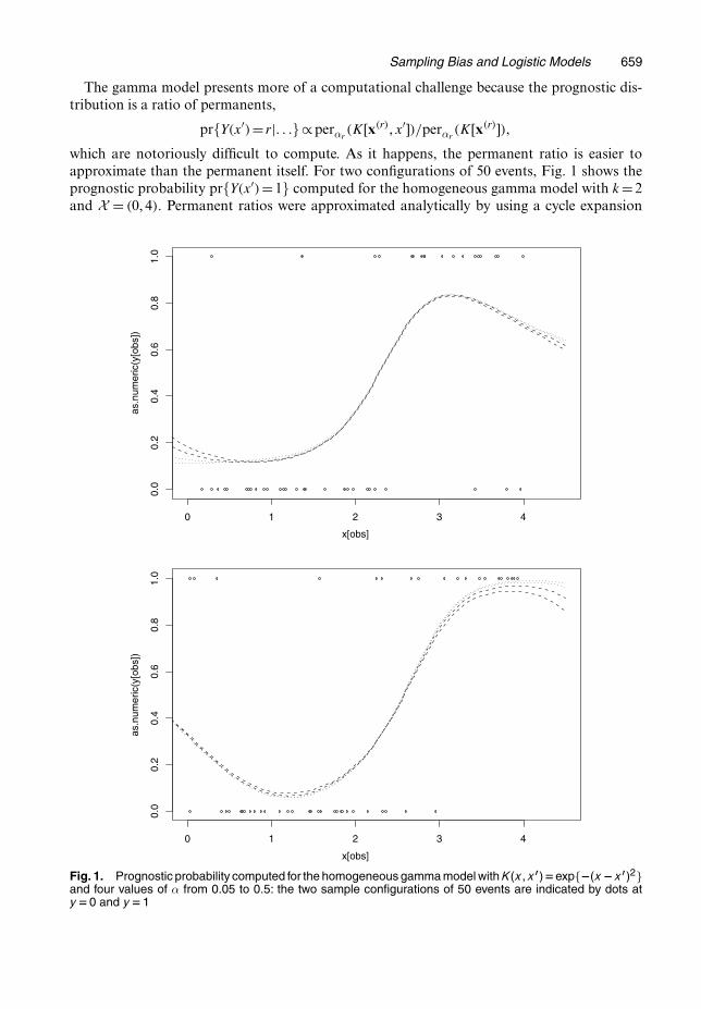
which are notoriously difficult to compute. As it happens, the permanent ratio is easier toapproximate than the permanent itself. For two configurations of 50 events, Fig. 1 shows theprognostic probability pr{Y.x′/=1} computed for the homogeneous gamma model with k =2and X = .0, 4/. Permanent ratios were approximated analytically by using a cycle expansion
0 1 2 3 4
0 1 2 3 4
0.0
0.2
0.4
0.6
0.8
1.0
x[obs]
as.n
umer
ic(y
[obs
])
0.0
0.2
0.4
0.6
0.8
1.0
x[obs]
as.n
umer
ic(y
[obs
])
Fig. 1. Prognostic probability computed for the homogeneous gamma model with K.x, x0/Dexp{�.x �x0/2}and four values of α from 0.05 to 0.5: the two sample configurations of 50 events are indicated by dots aty D0 and y D1
660 P. McCullagh
truncated after cycles of length 4. In the homogeneous gamma model, the one-dimensionalconditional probability q1.y = 1|x/ for a single event is 1
2 for every x, so the prognostic proba-bility graphs in Fig. 1 should not be confused with regression curves.
8. Summarizing remarks
8.1. Conventional random-effects modelsThe statistical model (3) has an observation space {0, 1}n for each sample of size n, and aparameter space with four components .α,β,σ, τ /. Everything else is incidental. The randomprocess η, used as an intermediate construct in the derivation of the distribution, is not a com-ponent of the observation space; nor is it a component of the parameter space. In principle,model (3) could have been derived directly without the intermediate step (2), so direct inferencefor η is impossible in model (3). On account of the consistency condition (5), we can computethe conditional probability of any event such as
E{Y.u′/|y}=E
[exp{α+βx′ +η.x′/}
1+ exp{α+βx′ +η.x′/}∣∣∣∣y
]= px,x′.y, 1/
px.y/, .16/
using the model distribution with an additional unit having x.u′/=x′. Sample space inferencesof this sort are accessible directly from model (3), but inference for η is not. Similar remarks applyto the Gaussian model (1), in which case the conditional expected value (16) is a generalizedsmoothing spline in x′.
Since the likelihood function does not determine the observation space, we look to the like-lihood function only for parameter estimation, not for inferences about the sample space orsubsequent values of the process. This interpretation of model and likelihood is neutral in theBayes–non-Bayes spectrum. It is consistent with expression (2) as a partially Bayesian modelwith parameters .α,β, η/, in which the Gaussian process serves as the prior distribution for η.The Bayesian formulation enables us to compute a posterior distribution for η.x′/ whether it isof interest or not. Despite the formal equivalence of expression (2) as a partially Bayesian model,and model (3) as a non-Bayesian model, the two formulations are different in a fundamental way.The treatment effect is ordinarily defined as the ratio of success odds for a treated individual tothat of an untreated individual having the same baseline covariate values. Because of parameterattenuation, the value that is obtained for the partially Bayesian model (2) is not the same asthat for the marginal model (3). Both calculations are unit specific, so this distinction is nota difference between subject-specific and population-averaged effects. This paper argues thatneither definition is appropriate because neither model accounts properly for sampling biases.
8.2. Subject-specific and population-average effectsFor all models considered in this paper, including (1)–(4), the probabilities are unit specific.That is to say, each regression model specifies the response distribution for every unit, andthe joint distribution for each finite subset of units. Treatment effect is measured by the oddsratio, which may vary from unit to unit depending on the covariate value. The population-average effect, if it is to be used at all, must be computed after the fact by averaging thetreatment effects over the distribution of x-values for the units in the target population. Notethe distinction between unit u and subject s.u/: two distinct units u and u′ in a crossover orlongitudinal design correspond to the same patient or subject if s.u/= s.u′/. This block struc-ture is assumed to be encoded in x.
Sampling Bias and Logistic Models 661
Numerous researchers have noted a close parallel between expression (2) and the one-dimen-sional marginal distributions that are associated with model (3). Specifically, if ηu is a zero-meanGaussian variable,
logit[pr{Y.u/=1|η; x}]=α+β x.u/+ηu .17/
implies
logit[pr{Y.u/=1; x}] αÅ +βÅ x.u/ .18/
by averaging over ηu for fixed u. Zeger et al. (1988) gave an accurate approximation for theattenuation ratio τ =βÅ=β�1, which depends on the variance of ηu. Neuhaus et al. (1991) con-firmed the accuracy of this approximation. They also gave a convincing demonstration of themagnitude of the attenuation effect by analysing a study of breast disease in two different ways.Maximum likelihood estimates α and β were obtained by maximizing an approximation to theintegral (3) by using the software package egret. The alternative, generalized estimating equa-tions using expression (18) for expected values supplemented by an approximate covariancematrix, gives estimates αÅ and β
Åof the attenuated parameters. The attenuation ratios βÅ=β
were found to be approximately 0.35, which is in good agreement with the Taylor approximation.In biostatistical terminology, the regression parameters α and β in equation (17) are called
subject specific or cluster specific, whereas the parameters in (18) are called population-averaged effects (Zeger et al., 1988). The terms ‘marginal parameterization’ (Glonek andMcCullagh, 1995), ‘marginal model’ (Heagerty, 1999) and even ‘marginalized model’ (Schildc-rout and Heagerty, 2007) are also used in connection with (18). Certainly, it is important todistinguish one from the other because the parameter values are very different. Nonetheless,the population-average terminology is misleading because both (17) and (18) refer to a specificunit labelled u, and hence to a specific subject s.u/, not to a randomly selected unit or subject.The bivariate and multivariate version (3) is also specific to the particular set of units havingcovariate configuration x. In other words, both of these are conventional regression models inwhich the concept of random sampling of units is absent.
Apart from minor differences introduced by approximating the one-dimensional integral by(18), and similar approximations for bivariate and higher order distributions, these are in fact thesame model. They have different parameterizations, and they use different methods to estimatethe parameters, but the distributions are the same. The distinction between the population-average approach and the cluster-specific approach is not a distinction between models, but adistinction between two parameterizations of essentially the same model, and two methods forparameter estimation.
Having established the point that there is only one regression model, it is necessary to focus onthe parameterizations and to ask which parameterization is most natural, and for what purpose.Heagerty (1999) pointed out that individual components of β in the subject-specific parame-terization are difficult to interpret unless the subject-specific effect ηu is known. Neuhaus et al.(1991), section 6, noted that, since each individual has her own latent risk, the model invitesan unwarranted causal interpretation. Galbraith (1991) criticized the interventionist interpre-tation of parameters in equation (17) and pointed out correctly that additional assumptionsare required to justify this interpretation in an observational study. If each pair of units havingdifferent treatment levels is necessarily a distinct pair of individuals or subjects, the treatmenteffect involves a comparison of distributions for two distinct subjects.
From this author’s point of view, ephemeral unit-specific, subject-specific or cluster-specificeffects such as {ηu} or η{x.u/} are best regarded as random variables rather than parameters,a distinction that is fundamental in statistical models. Given the parameters, the conventional

662 P. McCullagh
model specifies the probability distribution for each unit and each set of units by integration.The intermediate step (17) shows a random variable arising in this calculation, leading to thejoint distribution (3) whose one-dimensional distributions are well approximated by expression(18). Two units u and u′ having the same baseline covariate values but different treatment levelshave different response distributions. The treatment effect is the difference between these proba-bilities, which is usually measured on the log-odds-ratio scale. Although established terminologysuggests otherwise, the treatment component of βÅ in expression (18) is the treatment effect thatis specific to this pair of units u and u′. If these units represent the same subject in a controlledcrossover design, an interventionist interpretation is appropriate. Otherwise, if two units havingdifferent treatment levels necessarily represent distinct subjects, βÅ is the difference of responseprobabilities for distinct subjects, so there can be no interventionist interpretation.
8.3. Implications for applicationsConsider a market research study of consumer preferences for a set of products such as breakfastcereals. The relevant information is extracted from a database in which each purchase event isrecorded together with the store information and consumer information. Breakfast cereal pur-chases are the relevant events. Following conventional notation, i denotes the purchase event, Yi
is the brand purchased and xi is a vector of covariates, some store specific and some consumerspecific. The aim is to study how the market share pr.Yi = r|xi = x/ depends on x, possibly byusing a multinomial response model of the form (4). The random effects may be associated withstore-specific variables such as geographic location, or consumer-specific variables such as ageor ethnicity. The treatment effect may be connected with pricing, product placement or localadvertising campaigns.
As I see it, the conventional paradigm of a stochastic process defined on a fixed set of unitsis indefensible in applications of this sort. Most purchase events are not purchases of breakfastcereals, so the relevant events (cereal purchases) are defined by selecting from the database thosethat are in the designated subset C. An arbitrary choice must be made regarding the inclusionof dual use materials such as grits and porridge oats. Rationally, the model must be defined forgeneral response sets, and we must then insist that the model for the subset C′ ⊂C be consistentwith the model for C. Consistency means only that the two models are non-contradictory; theyassign the same probability to equivalent events. The evolving population model with a fixedobservation period is consistent under class restriction, but the conventional logistic model (4)with random effects is not.
The notation used above is conventional but ambiguous. The market share of brand r instratum x is the limiting fraction of events in stratum x that are of class r, which is λr.x/=λ•.x/
for both model (4) and the evolving population model. The expected market share is the stratumprobability pr.Yi = r|i: xi =x/, which may be different from the conditional probability given xi
for fixed i. However, the central concept of a fixed unit i is clearly nonsense in this context, sothe standard interpretation of pr.Yi = r|xi =x/ for fixed i is unsatisfactory.
The situation described above arises in numerous areas of application such as studies ofanimal behaviour, studies of crime patterns, studies of birth defects and the classification ofbitmap images of handwritten decimal digits. The events are animal interactions, crimes, birthdefects and bitmap images. The response is the type of event, so C is a set of behaviours, crimetypes, birth defects or the 10 decimal digits. This set is exhaustive only in the sense that eventsof other types are excluded: hence the need for consistency under class restriction.
In the biostatistical literature, which deals exclusively with hierarchical models, an expressionsuch as E.Yi|Xi =x/ is usually described as a conditional expectation but is often interpreted asthe marginal mean response for those units i such that Xi =x. I do not mean to be unduly critical
Sampling Bias and Logistic Models 663
here because there can be no ambiguity if these averages are equal, as they are in a hierarchicalmodel for an exchangeable process. For an autogenerated process, these averages are usuallydifferent. It is not easy to make sense of the literature in this broader context given that onesymbol is used for two distinct purposes. To make the hierarchical formulation compatible withthe broader context of the evolving population model, it is necessary to interpret models (3)and (4) as stratum distributions, not conditional distributions. Once the distinction has beenmade, it is immediately apparent that the stratum distribution does not determine the condi-tional probability given x for a sequential sample. Consequently, probability calculations usingthe stratum distribution, and efforts to estimate the parameters by using the wrong likelihoodfunction (3), must be abandoned.
8.4. Sampling biasThe main thrust of this paper is that, when the units are unlabelled and sampling effects areproperly taken into account by using the evolving population model as described in Sections 3,5.4 and 7.1, there is no parameter attenuation. If the intensities are such that λ1.x/ has the samemean as exp.α+βx/λ0.x/, the correct version of expressions (17) and (18) for an autogeneratedunit u∈Zt is
logit[pr{Y.u/=1|λ, u∈Zt}]= log[λ1{x.u/}]− log[λ0{x.u/}]
=α+β x.u/+η{x.u/},
logit[pr{Y.u/=1|u∈Zt}]= log[m1{x.u/}]− log[m0{x.u/}]
=α+β x.u/,
with no approximation and no attenuation. The distinction made in Section 8.2 between twoparameterizations is simply incorrect for autogenerated units.
The subject-specific approach takes aim at the right target parameter in equation (17), butthe conventional likelihood or hierarchical Bayesian calculation leads to inconsistency whensampling bias is ignored in the steps leading to model (3). Sample x-values occur preferentiallyat points where the total intensity λ•.·/ is high, which is not so for a predetermined x. As aresult, parameter estimates from model (6) are inflated by the factor 1=τ where τ is the apparentattenuation factor. The inflation factor reported by Neuhaus et al. (1991) is a little less than3, so the bias in parameter estimates is far from negligible. The population-average procedurecommits the same error twice, by first defining the stratum probability ρ.x/ as the target, andthen failing to recognize that E.Y |x/ =ρ.x/ for a random sample. But a fortuitous ambiguity ofthe conventional notation E.Y |x/ allows it to estimate the right parameter π.x/ consistently byestimating the wrong parameter ρ.x/ inconsistently.
For a sequential sample, the parameters α and β in equation (17) are exactly equal tothe parameters αÅ and βÅ in the marginal distribution (18). The apparent attenuation arisesnot because of a real distinction between subject-specific and population-averaged effects,but because of failure to recognize and make allowance for sampling effects in the statisticalmodel.
Acknowledgements
I am grateful to the referees for helpful comments on an earlier version, and to J. Yang for theR code that was used to produce Fig. 1.
Support for this research was provided by National Science Foundation grant DMS-0305009.
664 Discussion on the Paper by McCullagh
References
Baddeley, A. and Jensen, E. B. (2005) Stereology for Statisticians. Boca Raton: Chapman and Hall.Besag, J. (1974) Spatial interaction and the statistical analysis of lattice systems (with discussion). J. R. Statist.
Soc. B, 36, 192–236.Besag, J. and Kempton, R. (1986) Statistical analysis of field experiments using neighbouring plots. Biometrics,
42, 231–251.Breslow, N. E. and Clayton, D. G. (1993) Approximate inference in generalized linear mixed models. J. Am.
Statist. Ass., 88, 9–25.Cox, D. R. (1958) Planning of Experiments. New York: Wiley.Cox, D. R. and Snell, E. J. (1979) On sampling and the estimation of rare errors. Biometrika, 66, 125–132.Galbraith, J. I. (1991) The interpretation of a regression coefficient. Biometrics, 47, 1593–1596.Glonek, G. F. V. and McCullagh, P. (1995) Multivariate logistic models. J. R. Statist. Soc. B, 57, 533–546.Green, P. and Silverman, B. (1994) Nonparametric Regression and Generalized Linear Models. London: Chapman
and Hall.Heagerty, P. J. (1999) Marginally specified logistic-normal models for longitudinal binary data. Biometrics, 55,
688–698.Laird, N. and Ware, J. (1982) Random effects models for longitudinal data. Biometrics, 38, 963–974.Lee, Y. and Nelder, J. A. (1996) Hierarchical generalized linear models (with discussion). J. R. Statist. Soc. B, 58,
619–678.Lee, Y., Nelder, J. A. and Pawitan, Y. (2006) Generalized Linear Models with Random Effects. London: Chapman
and Hall.Liang, K.-Y. and Zeger, S. L. (1986) Longitudinal data analysis using generalised linear models. Biometrika, 73,
13–22.McCullagh, P. (1983) Quasi-likelihood functions. Ann. Statist., 11, 59–67.McCullagh, P. (2005) Exchangeability and regression models. In Celebrating Statistics (eds A. C. Davison,
Y. Dodge and N. Wermuth), pp. 89–113. Oxford: Oxford University Press.McCullagh, P. and Møller, J. (2006) The permanental process. Adv. Appl. Probab., 38, 873–888.McCullagh, P. and Nelder, J. A. (1989) Generalized Linear Models, 2nd edn. London: Chapman and Hall.McCullagh, P. and Yang, J. (2006) Stochastic classification models. In Proc. Int. Congr. Mathematicians, vol. III
(eds M. Sanz-Solé, J. Soria, J. L. Varona and J. Verdera), pp. 669–686. Zurich: European Mathematical SocietyPublishing House.
McCulloch, C. E. (1994) Maximum likelihood variance components estimation in binary data. J. Am. Statist.Ass., 89, 330–335.
McCulloch, C. E. (1997) Maximum-likelihood algorithms for generalized linear mixed models. J. Am. Statist.Ass., 92, 162–170.
Møller, J., Syversveen, A. R. and Waagepetersen, R. P. (1998) Log Gaussian Cox processes. Scand. J. Statist., 25,451–482.
Neuhaus, J. M., Kalbfleisch, J. D. and Hauck, W. W. (1991) A comparison of cluster-specific and population-averaged approaches for analyzing correlated binary data. Int. Statist. Rev., 59, 25–35.
Schall, R. (1991) Estimation in generalized linear models with random effects. Biometrika, 78, 719–727.Schildcrout, J. S. and Heagerty, P. J. (2007) Marginalized models for moderate to long series of longitudinal binary
response data. Biometrics, 63, 322–331.Shirai, T. and Takahashi, Y. (2003) Random point fields associated with certain Fredholm determinants, I:
fermion, Poisson and boson point processes. J. Functnl Anal., 205, 414–463.Wahba, G. (1985) A comparison of GCV and GML for choosing the smoothing parameter in the generalized
spline smoothing problem. Ann. Statist., 13, 1378–1402.Wolfinger, R. W. (1993) Laplace’s approximation for nonlinear mixed models. Biometrika, 80, 791–795.Zeger, S. L. and Liang, K.-Y. (1986) Longitudinal data analysis for discrete and continuous outcomes. Biometrics,
42, 121–130.Zeger, S. L., Liang, K.-Y. and Albert, J. A. (1988) Models for longitudinal data: a generalized estimating equations
approach. Biometrics, 44, 1049–1060.
Discussion on the paper by McCullagh
N. T. Longford (SNTL, Reading, and Universitat Pompeu Fabra, Barcelona)Linear regression of a single outcome variable is a key univariate method for studying what is essentiallya multivariate setting of the outcome and one or several covariates. This paper finds a severe limitationto this univariateness in the context of logistic regression for correlated outcomes. It informs us of thenon-ignorability of the process by which the values of the covariates are generated; by sampling (exceptfor a special case), assignment or a mechanism of another kind.
Discussion on the Paper by McCullagh 665
−4
−2
42
0
X
logi
t
0 5 0 5
0.0
0.5
1.0
X(a) (b)
Pro
babi
lity
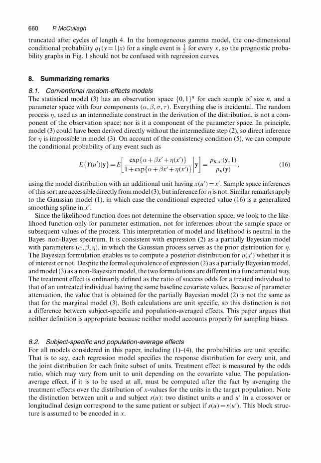
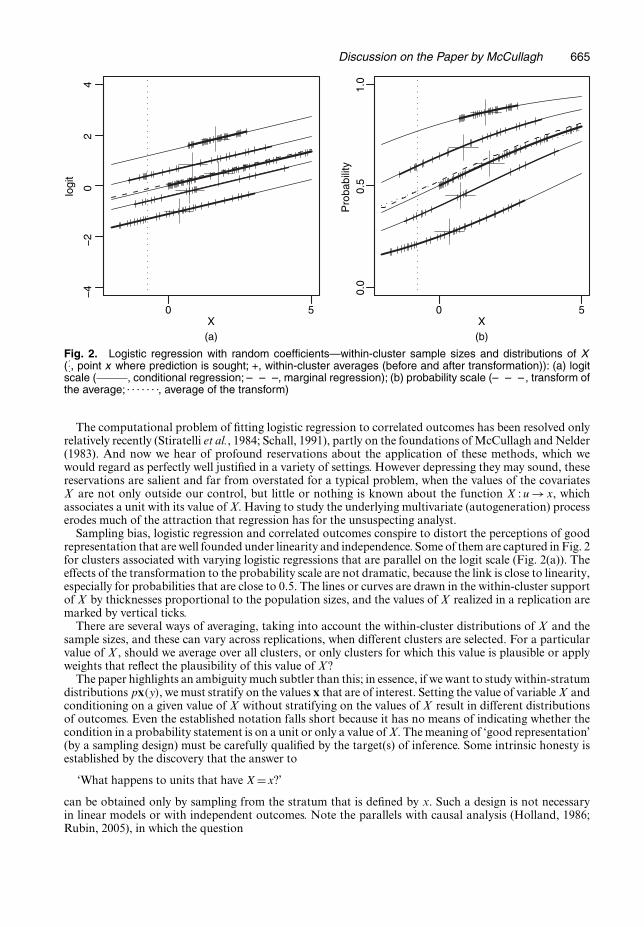
Fig. 2. Logistic regression with random coefficients—within-cluster sample sizes and distributions of X(:::, point x where prediction is sought; +, within-cluster averages (before and after transformation)): (a) logit
scale ( , conditional regression; – – –, marginal regression); (b) probability scale (– – –, transform ofthe average; . . . . . . ., average of the transform)
The computational problem of fitting logistic regression to correlated outcomes has been resolved onlyrelatively recently (Stiratelli et al., 1984; Schall, 1991), partly on the foundations of McCullagh and Nelder(1983). And now we hear of profound reservations about the application of these methods, which wewould regard as perfectly well justified in a variety of settings. However depressing they may sound, thesereservations are salient and far from overstated for a typical problem, when the values of the covariatesX are not only outside our control, but little or nothing is known about the function X : u → x, whichassociates a unit with its value of X. Having to study the underlying multivariate (autogeneration) processerodes much of the attraction that regression has for the unsuspecting analyst.
Sampling bias, logistic regression and correlated outcomes conspire to distort the perceptions of goodrepresentation that are well founded under linearity and independence. Some of them are captured in Fig. 2for clusters associated with varying logistic regressions that are parallel on the logit scale (Fig. 2(a)). Theeffects of the transformation to the probability scale are not dramatic, because the link is close to linearity,especially for probabilities that are close to 0.5. The lines or curves are drawn in the within-cluster supportof X by thicknesses proportional to the population sizes, and the values of X realized in a replication aremarked by vertical ticks.
There are several ways of averaging, taking into account the within-cluster distributions of X and thesample sizes, and these can vary across replications, when different clusters are selected. For a particularvalue of X , should we average over all clusters, or only clusters for which this value is plausible or applyweights that reflect the plausibility of this value of X ?
The paper highlights an ambiguity much subtler than this; in essence, if we want to study within-stratumdistributions px.y/, we must stratify on the values x that are of interest. Setting the value of variable X andconditioning on a given value of X without stratifying on the values of X result in different distributionsof outcomes. Even the established notation falls short because it has no means of indicating whether thecondition in a probability statement is on a unit or only a value of X. The meaning of ‘good representation’(by a sampling design) must be carefully qualified by the target(s) of inference. Some intrinsic honesty isestablished by the discovery that the answer to
‘What happens to units that have X=x?’
can be obtained only by sampling from the stratum that is defined by x. Such a design is not necessaryin linear models or with independent outcomes. Note the parallels with causal analysis (Holland, 1986;Rubin, 2005), in which the question
666 Discussion on the Paper by McCullagh
‘What would happen if the unit had a different value of x?’
can be inferred without any assumptions only when we can assign values of X to units (e.g. by randomi-zation).
The results about the sampling protocols in Section 3 can be interpreted as failed attempts (not theauthor’s failures!) at exchanging, mentally or analytically, two operations (ratio and expectation) whichcommute under linearity or certainty, but not otherwise. But in the mental processes these two operationsare difficult to identify.
In most applications, quotas for the values of X cannot be enforced, and so we must study the processthat generates the values of X. I think that the proposed models of evolving population are but models,i.e. they inject some realism into the analysis but do not make the bias disappear. In any case, the choicebetween the available options is not trivial for a secondary analyst who has modest resources to study asampling process that may have involved some improvisation and the details of which are poorly recorded.
The paper is concerned solely with bias, which asymptotically dominates the mean-squared error ininferences with invalid models and assumptions. Parsimony is valuable with small samples, because itpromotes smaller sampling variation. The inevitable uncertainty that will arise as we study and model theprocess that generates the values of x may bring about a variance inflation that is in excess of the squaredbias. There is therefore some scope for compromise, to use models that are not valid but are associatedwith only limited bias. We should not pretend that such models are valid, but estimate the squared biasincurred or seek an upper bound for it. Some avenues for this are implied in the paper and I think thattheir elaboration would be useful.
I conclude by proposing the vote of thanks for this excellent paper.
Peter J. Diggle (Lancaster University and Johns Hopkins University, Baltimore)At a very simple level, this paper is a plea for precision of notation. At a slightly deeper level, it warns usagainst indulging in statistical modelling without respecting the study design. At a considerably deeperlevel, it challenges conventional wisdom regarding the widespread use of unobserved random variablesas fundamental building-blocks in what are variously called random effects, latent variable, multilevel orhierarchical models.
I agree with Peter McCullagh that confusion can easily arise through the use of the same everyday word‘given’, and the same accompanying notation, to mean any one of three quite different things: fixing thevalue of a non-random variable; conditioning on the realized value of a random variable; indexing a familyof distributions by the value of a parameter (although Bayesians may regard the second and third as beingequivalent). I would agree with Peter McCullagh’s use of px.y/ for the first of these, reserving p.y|x/ forthe second. For the third, I favour p.y; θ/ because we often use θ as the argument of a function, e.g.a likelihood.
The importance of good study design can never be overemphasized, and the same surely applies tothe need to respect the study design when analysing the data. This is not an argument for accepting onlyinferences that are purely design based. But there is a difference between an unverifiable assumption and anassumption that is palpably false, and Peter McCullagh has shown us that, if we pretend that a stochasticsampling process is a prespecified study design, we can get ourselves into serious trouble.
I have lately taken an interest in this question in the specific setting of geostatistical modelling. There,the data in their simplest form consist of responses Yi : i=1, . . . , n associated with locations xi ∈A, whereA is a spatial region of interest. Typically, the Yi are considered to be noisy measurements of the valueat xi of a spatial process S.x/ : x ∈ R2. A widely used model is that Yi|S.·/ ∼ N{β+ S.xi/,σ2}, the Yi areconditionally independent given S.·/ and S.·/ is a zero-mean Gaussian process. Standard geostatisticalmethods assume, if only implicitly, that x is either a non-random variable or is stochastically independentof S.·/. But not infrequently this assumption is false. For example, in environmental monitoring networksthe design prescription for the monitoring locations is rarely stated but in a rather vague sense will typicallyplace monitors in areas that are suspected to be highly polluted. To investigate the implications of this, weextend our notation to include a point process of locations X , in addition to a measurement process Y ,and an underlying spatial signal S, and adopt the notation [·] for ‘the distribution of’. Then, the standardgeostatistical model can be written as
[S, X, Y ]= [S] [X|S] [Y |X, S]= [S] [X]∏
[Yi|S.Xi/]
and conditioning on [X] is innocuous for inference about S and/or Y. In contrast, for preferentially sampledgeostatistical data, the model becomes
Discussion on the Paper by McCullagh 667
[S, X, Y ]= [S] [X|S] [Y |X, S]= [S] [X|S]∏
[Yi|S.Xi/]:
The likelihood for the data X and Y is now∫[S] [X|S]
∏[Yi|S.Xi/] dS
and conditioning on X is not the right thing to do. The consequences of this are explored in Diggle et al.(2008).
Similar issues arise in longitudinal studies, e.g. when study participants deviate from their assigned fol-low-up protocol for reasons unknown; see, for example, Lin et al. (2004), Lipsitz et al. (2002) or Sun et al.(2007).
Returning to Peter McCullagh’s main focus of attention, the logistic regression model with a randomeffect added to the linear predictor, I accept that this model is overused, but to state that ‘efforts to estimatethe parameters by using the wrong likelihood (3) must be abandoned’ (my italics) seems a little sweeping.A possible interpretation of model (3), when values of explanatory variables are not prespecified, is asfollows. We assume an incomplete model
logit{P.Y =1|X, U/}=α+βX+γU
for the random vector .Y , X, U/ and wish to make inferences about β. We are unable to observe U butuse independent random sampling from the population of interest to obtain data .yi, xi/, i = 1, . . . , n.A complete-model specification takes the form
[Y , X, U]= [Y |X, U] [X|U] [U]: .19/
We have no interest in the distributions of X or of U but are willing to assume a parametric form for thedistribution of U induced by the random sampling design. If, additionally, we assume that X and U areindependent, then in equation (19) we can condition on X and marginalize with respect to U , resulting inthe likelihood ∫
[Y |X, U] [U] dU,
which is distribution (3). In most discussions of random-effects models the assumption that X and U areindependent is left unstated and is probably unrealistic in many applications. But if this assumption ismade explicit, and thereby open to criticism, I can see no logical objection to the use of model (3).
As always, Peter McCullagh has challenged us to think very carefully about matters of fundamentalimportance in the application of the statistical method to substantive problems. I am very pleased indeedto second the vote of thanks.
The vote of thanks was passed by acclamation.
John Nelder (Imperial College London)Underneath equation (3), which defines the marginal likelihood after integrating out the random effects,the author states ‘The word model refers to these distributions’. To me this seems to give a very restrictiveclass of random-effect models, in which the random effects are used only to produce overdispersion in thedistribution of the responses. The author’s definition does not allow the random effects to be estimated(a word which I prefer to ‘predicted’) and hence there is no way of checking whether their distributionsatisfies what has been assumed in setting up the model. I regard such models as inherently defective fromthe model fitting point of view.
In seeking to deal with these problems, while keeping to a likelihood type of inference, Lee et al. (2006)were led to extend Fisher likelihood (of which equation (3) is an example) to produce an extended likeli-hood in which random effects could appear. We are well aware that the theory underlying inferences fromthis extended likelihood (or, more exactly, the h-likelihood that is derived from it) is as yet incomplete, butextensive simulation on a wide variety of models from the class of double hierarchical generalized linearmodels has shown consisently good results, as measured by bias and mean-squared error. The algorithmfor fitting these models reduces to a set of interconnected generalized linear models, each using iterativeweighted least squares. We allow random effects to appear in the linear predictors of either mean or disper-sion or both, and to have distributions belonging to any exponential family conjugate distribution. Given
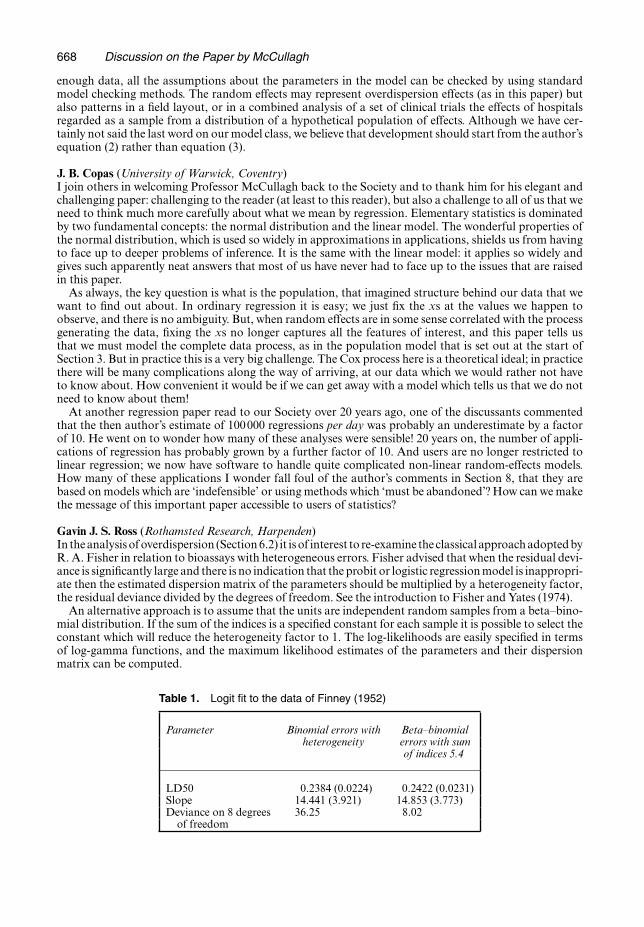
668 Discussion on the Paper by McCullagh
enough data, all the assumptions about the parameters in the model can be checked by using standardmodel checking methods. The random effects may represent overdispersion effects (as in this paper) butalso patterns in a field layout, or in a combined analysis of a set of clinical trials the effects of hospitalsregarded as a sample from a distribution of a hypothetical population of effects. Although we have cer-tainly not said the last word on our model class, we believe that development should start from the author’sequation (2) rather than equation (3).
J. B. Copas (University of Warwick, Coventry)I join others in welcoming Professor McCullagh back to the Society and to thank him for his elegant andchallenging paper: challenging to the reader (at least to this reader), but also a challenge to all of us that weneed to think much more carefully about what we mean by regression. Elementary statistics is dominatedby two fundamental concepts: the normal distribution and the linear model. The wonderful properties ofthe normal distribution, which is used so widely in approximations in applications, shields us from havingto face up to deeper problems of inference. It is the same with the linear model: it applies so widely andgives such apparently neat answers that most of us have never had to face up to the issues that are raisedin this paper.
As always, the key question is what is the population, that imagined structure behind our data that wewant to find out about. In ordinary regression it is easy; we just fix the xs at the values we happen toobserve, and there is no ambiguity. But, when random effects are in some sense correlated with the processgenerating the data, fixing the xs no longer captures all the features of interest, and this paper tells usthat we must model the complete data process, as in the population model that is set out at the start ofSection 3. But in practice this is a very big challenge. The Cox process here is a theoretical ideal; in practicethere will be many complications along the way of arriving, at our data which we would rather not haveto know about. How convenient it would be if we can get away with a model which tells us that we do notneed to know about them!
At another regression paper read to our Society over 20 years ago, one of the discussants commentedthat the then author’s estimate of 100000 regressions per day was probably an underestimate by a factorof 10. He went on to wonder how many of these analyses were sensible! 20 years on, the number of appli-cations of regression has probably grown by a further factor of 10. And users are no longer restricted tolinear regression; we now have software to handle quite complicated non-linear random-effects models.How many of these applications I wonder fall foul of the author’s comments in Section 8, that they arebased on models which are ‘indefensible’ or using methods which ‘must be abandoned’? How can we makethe message of this important paper accessible to users of statistics?
Gavin J. S. Ross (Rothamsted Research, Harpenden)In the analysis of overdispersion (Section 6.2) it is of interest to re-examine the classical approach adopted byR. A. Fisher in relation to bioassays with heterogeneous errors. Fisher advised that when the residual devi-ance is significantly large and there is no indication that the probit or logistic regression model is inappropri-ate then the estimated dispersion matrix of the parameters should be multiplied by a heterogeneity factor,the residual deviance divided by the degrees of freedom. See the introduction to Fisher and Yates (1974).
An alternative approach is to assume that the units are independent random samples from a beta–bino-mial distribution. If the sum of the indices is a specified constant for each sample it is possible to select theconstant which will reduce the heterogeneity factor to 1. The log-likelihoods are easily specified in termsof log-gamma functions, and the maximum likelihood estimates of the parameters and their dispersionmatrix can be computed.
Table 1. Logit fit to the data of Finney (1952)
Parameter Binomial errors with Beta–binomialheterogeneity errors with sum
of indices 5.4
LD50 0.2384 (0.0224) 0.2422 (0.0231)Slope 14.441 (3.921) 14.853 (3.773)Deviance on 8 degrees 36.25 8.02
of freedom

Discussion on the Paper by McCullagh 669
As an example of this analysis, the data that were used by Finney (1952) in his Table 10 may be fitted byusing logits rather than probits, with the results that are given in Table 1 (with estimated standard errorsin parentheses).
As the sum of beta-indices is progressively reduced the estimated variances increase. The likelihoodcontours in parameter space are slightly different for the two approaches, but Fisher’s approach appearsto be quite adequate for practical purposes.
Jesper Møller (Aalborg University)I welcome this stimulating paper, with its use of point process models for discussing sampling bias inregression models. The central model is a Cox process model evolving in time t and with marks .y, x/,where y is a response taking values in a finite set and x is a spatial location. It is driven by an intensity ofthe form λy.x/ ν.dx/ dt, with a particular focus on log-Gaussian models or gamma models for the randomfunctions λy.x/. Note that the marks .yi, xi/ are independent of the times ti. As discussed below, otherpoint process models could be of relevance.
Could other types of Cox models be included? Shot noise Cox processes (e.g. Møller (2003)) are, incontrast with log-Gaussian models (Section 5. 2), closed under aggregation, whereas moment expressionsare less simple (e.g. Møller and Waagepetersen (2003)). Furthermore, McCullagh’s random intensity maybe extended to the time inhomogeneous case λy.x/ ν.dx/ κ.dt/, say, so that, for example, quota samplingremains unbiased.
Another important class of point process models with marks is based on modelling the conditionalintensity, i.e. when we at time t condition on the history of the evolving process (e.g. Daley and Vere-Jones(2003)). For example, expressions for the unconditional and conditional distributions considered underthe various sampling protocols in Section 3.2 and the limit distribution in Section 4 will be of a simi-lar form to that in McCullagh’s paper. In particular, if the marks .yi, xi/ are independent of the times tiand distributed as in McCullagh’s Cox model, we again obtain equation (6), and hence quota samplingis unbiased under the log-Gaussian model that is specified a few lines after equation (6), and we stillobtain the limiting low intensity conditional distribution in equation (11), and so the theory in Section 5applies.
For spatial point process modelling, the analogy with generalized linear models and random-effectsmodels is to some extent discussed in Møller and Waagepetersen (2007).
The following contributions were received in writing after the meeting.
D. R. Cox (Nuffield College, Oxford)Professor McCullagh’s challenging paper on an important topic raises, implicitly or explicitly, many issues,in particular about generalized linear mixed models, especially those of logistic form.
It is natural to compare analyses of these logistic models with the corresponding analysis-of-covariancetable (Wilsdon (1934), appendix A). Analysis, at least informally, of parallelism and of possible systematicdepartures from parallelism seems important for interpretation. Further the notion of two regressions, onewithin and the other between study individuals, may be relevant. These issues seem not much discussed inthe more recent literature.
If the choice of individuals for study is not conditionally independent of outcome given the explanatoryvariables it is clear that careful analysis of the selection process is essential and the elegant discussion in thepaper of the connection with point processes is very interesting. It would be valuable to see more explicitdevelopment in terms of one or two specific examples. Some of those sketched in the paper are not entirelyconvincing. For example, fibres in a traditional textile yarn are identified in principle by the position oftheir ‘left’ end, thus providing a sampling frame, and careful methods of sampling either respect that orintroduce appropriate corrections. Selection of patients in a clinical trial seems broadly similar except forthe issue of non-compliance. Non-compliance arising during a study has been quite extensively studied.So far as I know, although it is widely recognized that the population of individuals involved, those givinginformed consent, deviates, possibly seriously, from the target population, there is little work on what, ifanything, can be done about non-compliance before entry. Can the ideas in the paper make a contributionto this particular version of non-compliance?
Ruth Keogh (University of Cambridge)I found Professor McCullagh’s paper very interesting and challenging and am interested in his views onextensions to different types of study.
670 Discussion on the Paper by McCullagh
In Section 3 the author discusses studies of associations between covariates and event occurrence in anevolving population and considers several sampling protocols which may be used to select the study units.The functions px.y/ and p.y|x/ which arise under different protocols are compared. The case–controldesign is one of the protocols considered and I find it interesting to compare McCullagh’s derivation of theconditional probability with the work of Prentice and Pyke (1979) and Farewell (1979), who establishedthe validity of analysing data obtained from a case–control study as though they had arisen prospectively.
Although the case–control design is discussed in the paper, the various cohort sampling designs thatare commonly used in epidemiological studies do not appear to be considered. Under cohort samplingschemes cases and controls are sampled from an underlying cohort taking account of event times. Thesampling may be performed during follow-up or retrospectively in a pre-existing cohort. I am interestedto hear any comments from the author regarding how the issues raised in the paper may extend to studiesusing cohort sampling designs.
Under the cohort sampling designs the set of cases to be studied is commonly taken to be all indi-viduals experiencing the event(s) of interest in a fixed time period. The identification of the cases thusseems essentially to follow the protocol in Section 3.2.3. Controls are selected according to one of sev-eral designs, including the nested case–control design using incidence density sampling (Goldstein andLangholz, 1992), the case–cohort design (Prentice, 1986), and more complex nested case–control designsusing countermatching or quota sampling, for example (Borgan et al., l995). The analysis of data arisingfrom epidemiological studies using cohort sampling designs differs from methods that are described in thepaper; whereas the probabilities under the models in the paper are unit specific this is not quite so underthe cohort sampling designs, in which the contribution to the likelihood from each case is conditional oncovariate values in the comparison set. The control sampling procedure is incorporated in the analysis byusing a weighted partial likelihood or pseudolikelihood. However, the way in which the cases arose doesnot appear to be considered. In light of the results in the paper, should we be concerned about the methodsthat are used to analyse data arising from cohort sampling designs?
Anthony Y. C. Kuk (National University of Singapore)The author is to be congratulated for proposing an evolving population framework to factor in the effectof sampling plan and for pointing out that, for most sampling plans, the conditional distribution p.y|x/is not the same as the regression function px.y/.
Analysis of clustered data with informative cluster size has received a fair amount of attention recently(Hoffman et al., 2001; Williamson et al., 2003; Benhin et al., 2005). An often-quoted example is periodon-tal disease data where the dental health of a person will affect both the disease status of teeth as well asthe number of teeth (cluster size) that a person has. I shall show how the simplest evolving populationmodel discussed in Section 6.1 can be modified to model situations with non-ignorable cluster sizes. Asin Section 6.1, we assume that, given λ, the number m of events in unit time is Poisson distributed withparameter λ. However, rather than letting the two components of λ, λ0 and λ1, be independent, we findit more appropriate for our purpose to model the joint distribution of .λ0,λ1/ via the marginal distribu-tion of their sum λ=λ0 +λ1 and the conditional distribution of λ1=λ given λ. We can think of λ as afrailty term that reflects the health condition of a person. Given λ, a plausible way to model the effectof λ on λ1 could be something like E.λ1=λ|λ/ = ξ exp.−βλ/, 0 < ξ< 1, β� 0, so that β= 0 correspondsto the case of ignorable cluster size and β> 0 will induce a negative correlation between cluster size anddisease status. The marginal probability of Y1 =1 in the k-variate distribution of .Y1, . . . , Yk/, k �1, canbe obtained as
pk.Y1 =1|m� k/=E
[{1−
k−1∑i=0
exp.−λ/λi
i!
}λ1
λ
]/E
{1−
k−1∑i=0
exp.−λ/λi
i!
}
=E
[{1−
k−1∑i=0
exp.−λ/λi
i!
}ξ exp.−βλ/
]/E
{1−
k−1∑i=0
exp.−λ/λi
i!
}
which can be expressed in terms of quantities like E{λi exp.−γλ/}=M.i/λ .−γ/ involving derivatives of the
moment-generating function of λ. A convenient case is gamma-distributed λ with easily differentiableMλ{t/= .1−θt/−α. As a demonstration, when αθ=10 (the mean cluster size), α=0:9372 (which is chosento make the probability of zero cluster size equal to 0.1), ξ=0:4 andβ=0:1, the first five pk.1/ are computedto be 0.184, 0.168, 0.153, 0.140 and 0.128, which decrease with cluster size, compared with pk.1/ ≡ 0:4when β=0. More generally, we can model λ by using the three-parameter family of distributions that was
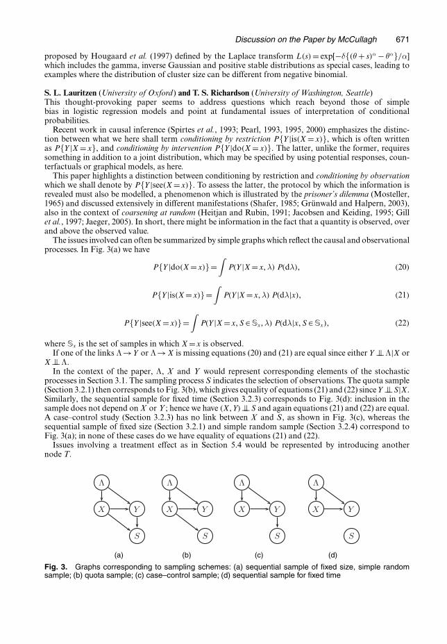
Discussion on the Paper by McCullagh 671
proposed by Hougaard et al. (1997) defined by the Laplace transform L.s/ = exp[−δ{.θ+ s/α − θα}=α]which includes the gamma, inverse Gaussian and positive stable distributions as special cases, leading toexamples where the distribution of cluster size can be different from negative binomial.
S. L. Lauritzen (University of Oxford) and T. S. Richardson (University of Washington, Seattle)This thought-provoking paper seems to address questions which reach beyond those of simplebias in logistic regression models and point at fundamental issues of interpretation of conditionalprobabilities.
Recent work in causal inference (Spirtes et al., 1993; Pearl, 1993, 1995, 2000) emphasizes the distinc-tion between what we here shall term conditioning by restriction P{Y |is.X = x/}, which is often writtenas P{Y |X = x}, and conditioning by intervention P{Y |do.X = x/}. The latter, unlike the former, requiressomething in addition to a joint distribution, which may be specified by using potential responses, coun-terfactuals or graphical models, as here.
This paper highlights a distinction between conditioning by restriction and conditioning by observationwhich we shall denote by P{Y |see.X=x/}. To assess the latter, the protocol by which the information isrevealed must also be modelled, a phenomenon which is illustrated by the prisoner’s dilemma (Mosteller,1965) and discussed extensively in different manifestations (Shafer, 1985; Grünwald and Halpern, 2003),also in the context of coarsening at random (Heitjan and Rubin, 1991; Jacobsen and Keiding, 1995; Gillet al., 1997; Jaeger, 2005). In short, there might be information in the fact that a quantity is observed, overand above the observed value.
The issues involved can often be summarized by simple graphs which reflect the causal and observationalprocesses. In Fig. 3(a) we have
P{Y |do.X=x/}=∫
P.Y |X=x,λ/ P.dλ/, .20/
P{Y |is.X=x/}=∫
P.Y |X=x,λ/ P.dλ|x/, .21/
P{Y |see.X=x/}=∫
P.Y |X=x, S ∈Sx,λ/ P.dλ|x, S ∈Sx/, .22/
where Sx is the set of samples in which X=x is observed.If one of the links Λ→Y or Λ→X is missing equations (20) and (21) are equal since either Y ⊥⊥Λ|X or
X⊥⊥Λ.In the context of the paper, Λ, X and Y would represent corresponding elements of the stochastic
processes in Section 3.1. The sampling process S indicates the selection of observations. The quota sample(Section 3.2.1) then corresponds to Fig. 3(b), which gives equality of equations (21) and (22) since Y ⊥⊥S|X.Similarly, the sequential sample for fixed time (Section 3.2.3) corresponds to Fig. 3(d): inclusion in thesample does not depend on X or Y ; hence we have .X, Y/⊥⊥S and again equations (21) and (22) are equal.A case–control study (Section 3.2.3) has no link between X and S, as shown in Fig. 3(c), whereas thesequential sample of fixed size (Section 3.2.1) and simple random sample (Section 3.2.4) correspond toFig. 3(a); in none of these cases do we have equality of equations (21) and (22).
Issues involving a treatment effect as in Section 5.4 would be represented by introducing anothernode T.
(a) (b) (c) (d)
Fig. 3. Graphs corresponding to sampling schemes: (a) sequential sample of fixed size, simple randomsample; (b) quota sample; (c) case–control sample; (d) sequential sample for fixed time
672 Discussion on the Paper by McCullagh
Youngjo Lee (Seoul National University)I congratulate the author on finding that sampling procedures could lead to distributions of random effectswithout attenuation in binomial hierarchical generalized linear models. Such attenuation in the behaviourof parameters between two models, if it occurs, is based on a failure to compare like with like (Lee andNelder, 2004). A question is whether the sampling model proposed is natural in biostatistics; for example,in a cohort study, the population base is defined at a moment in time.
It is often not clearly stated what we model, but in random-effect models we model p.y|x, η/, ratherthan p.y|η/ in model (2), leading to p.y|x/ via the integration (3). In my notation p.y|x, η/ = pθ.y|x, η/where the suffix θ is a parameter, which is suppressed for simplicity. When η.·/ is a known monotonefunction such as η.x/ = β0 + xβ1, we have p.y|x, η/ = pβ0,β1 .y|η/ = pβ0,β1 .y|x/, so that all p.y|x/, p.y|η/and p.y|x, η/ give an equivalent model. However, if a functional form of η.·/ is totally unknown it wouldbe natural to model p.y|x, η/ for the random-effect model (2). Even if we could make a full joint modelp.y, x|η/=p.y|x, η/ p.x|η/, information would be hardly recoverable from p.x|η/ because of the infinitedimensional parameter space of η. Thus, we model p.y|x, η/.
Many interesting random-effect models have been proposed which involve modelling of unobservablessuch as random effects. We do not agree that the use of an integrated likelihood is non-Bayesian, whereas anunintegrated likelihood is Bayesian. The extended likelihood principle of Bjørnstad (1996) states that theevidence for unobservables is contained in the extended likelihood such as the h-likelihood, and ProfessorNelder and I have shown how efficient inferences can be made from it, without resorting to estimatingequations. The random-effect model is not just an intermediate for the marginal model. It can also beused for various purposes, such as robust estimation for generalized linear model classes, deriving newsandwich estimators, imputation, animal breeding, smoothing and image recovery. . . (Lee et al., 2006).
Xiao-Li Meng (Harvard University, Cambridge)It seems trite to reiterate the importance of identifying the data-generating mechanism for proper analysis,especially in a top statistical journal. Yet McCullagh’s paper shows how easy it is to overlook such issues,even by many professional statisticians and for methods as well studied as logistic regression.
McCullagh is extremely careful with notation: p.y|x/ versus px.y/ and E.yu|xu =x/ versus E.yu|u, xu =x/.The importance of avoiding ‘dangerously ambiguous’ notation indeed cannot be overstated. McCullagh’sformulation avoids the notion of units, but even without this advance a more explicit notation wouldclearly remind us of the importance of the data-generating mechanism. Let {.yi, xi/, i = 1, . . . , n} be theobserved values of .Y , X/ from a population. To model them, we typically write P.yi, xi/, forgetting that itshould really be P.yi, xi|Oi =1/, where Oi is a Bernoulli variable indicating whether the ith subject’s .Y , X/are recorded and observed by the investigator. With this notation, few statisticians would miss the distinctionbetween P.Y |X, O=1/, similar to McCullagh’s stratum distribution, and P.Y |X/, the distribution of inter-est. The two are the same if, and only if, Y and O are conditionally independent given X. This conditionalindependence is sometimes referred to as the ignorability of sampling mechanism in survey literature. Inthe context of missing data, a perfect example of ‘autogenerated data’, this conditional independence iskey to ensuring an ignorable missing data mechanism (e.g. Rubin (1976)).
An on-going longitudinal study of young women’s sexual behaviour and risks highlights well the criticalimportance of recognizing the conditioning on O. The study asks each subject to keep a diary to recordher daily sexual activities and risks (if she had sexual intercourse, used a condom, whether the condombroke, etc.). Currently the shortest follow-up is about 3 years and the longest is about 7 years. However,as the study continues, the investigators are increasingly worried about the possibility that the very act ofkeeping a detailed diary could have changed a woman’s sexual behaviour or risk exposure, since recordingserves as a daily reminder, i.e. P.Y |X, O = 1/ potentially can be very different from P.Y |X, O = 0/. Theproblem was posed to me recently as a challenge: P.Y |X, O=0/ is logically impossible to estimate becauseif a woman did not keep a diary then the investigator would have no data! Although there is no spacehere to detail my brilliant solution (in the style of Pierre de Fermat), clearly carrying the ‘O’ notation atleast helps to prevent a long ‘Oops’ when inferring from the study to the general population of youngwomen.
Paul Rathouz (University of Chicago)Professor McCullagh has provided an interesting perspective on sampling models for binary data in thepresence of heterogeneity. His notion of ‘autogenerated units’ is applicable in epidemiologic studies ofdisease incidence. Here, I explore application of his ideas to case–control studies (Rothman (1986), page 62).I ask whether and how, in the presence of heterogeneity, data generated via case–control designs and
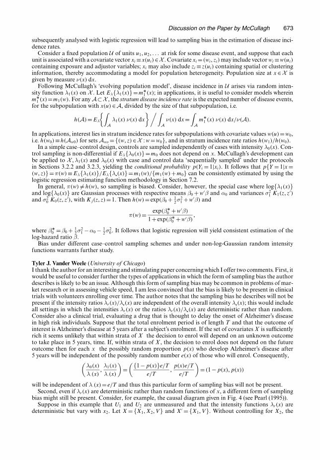
Discussion on the Paper by McCullagh 673
subsequently analysed with logistic regression will lead to sampling bias in the estimation of disease inci-dence rates.
Consider a fixed population U of units u1, u2, . . . at risk for some disease event, and suppose that eachunit is associated with a covariate vector xi ≡x.ui/∈X . Covariate xi = .wi, zi/ may include vector wi ≡w.ui/containing exposure and adjustor variables; xi may also include zi ≡ z.ui/ containing spatial or clusteringinformation, thereby accommodating a model for population heterogeneity. Population size at x ∈X isgiven by measure ν.x/ dx.
Following McCullagh’s ‘evolving population model’, disease incidence in U arises via random inten-sity function λ1.x/ on X . Let Eλ{λ1.x/}=mÅ
1 .x/; in applications, it is useful to consider models whereinmÅ
1 .x/=m1.w/. For any A⊂X , the stratum disease incidence rate is the expected number of disease events,for the subpopulation with x.u/∈A, divided by the size of that subpopulation, i.e.
h.A/=Eλ
{∫Aλ1.x/ ν.x/ dx
}/∫Aν.x/ dx=
∫A
mÅ1 .x/ ν.x/ dx=ν.A/:
In applications, interest lies in stratum incidence rates for subpopulations with covariate values w.u/=w0,i.e. h.w0/≡h.Aw0/ for sets Awo ={.w, z/∈X : w =w0}, and in stratum incidence rate ratios h.w1/=h.w0/.
In a simple case–control design, controls are sampled independently of cases with intensity λ0.x/. Con-trol sampling is non-differential if Eλ{λ0.x/}=m0 does not depend on x. McCullagh’s development canbe applied to X ,λ1.x/ and λ0.x/ with case and control data ‘sequentially sampled’ under the protocolsin Sections 3.2.2 and 3.2.3, yielding the conditional probability p.Yi = 1|xi/. It follows that p{Y = 1|x =.w, z/}=π.w/≡Eλ{λ1.x/}=Eλ{λ•.x/}=m1.w/={m1.w/+m0} can be consistently estimated by using thelogistic regression estimating function methodology in Section 7.2.
In general, π.w/ = h.w/, so sampling is biased. Consider, however, the special case where log{λ1.x/}and log{λ0.x/} are Gaussian processes with respective means β0 + w′β and α0 and variances σ2
1 K1.z, z′/and σ2
0 K0.z, z′/, with Kj.z, z/=1. Then h.w/= exp.β0 + 12σ
21 +w′β/ and
π.w/= exp.βÅ0 +w′β/
1+ exp.βÅ0 +w′β/
,
where βÅ0 =β0 + 1
2σ21 −α0 − 1
2σ20 . It follows that logistic regression will yield consistent estimation of the
log-hazard ratio β.Bias under different case–control sampling schemes and under non-log-Gaussian random intensity
functions warrants further study.
Tyler J. Vander Weele (University of Chicago)I thank the author for an interesting and stimulating paper concerning which I offer two comments. First, itwould be useful to consider further the types of applications in which the form of sampling bias the authordescribes is likely to be an issue. Although this form of sampling bias may be common in problems of mar-ket research or in assessing vehicle speed, I am less convinced that the bias is likely to be present in clinicaltrials with volunteers enrolling over time. The author notes that the sampling bias he describes will not bepresent if the intensity ratios λr.x/=λ•.x/ are independent of the overall intensity λ•.x/; this would includeall settings in which the intensities λr.x/ or the ratios λr.x/=λ•.x/ are deterministic rather than random.Consider also a clinical trial, evaluating a drug that is thought to delay the onset of Alzheimer’s diseasein high risk individuals. Suppose that the total enrolment period is of length T and that the outcome ofinterest is Alzheimer’s disease at 5 years after a subject’s enrolment. If the set of covariates X is sufficientlyrich it seems unlikely that within strata of X the decision to enrol will depend on an unknown outcometo take place in 5 years, time. If, within strata of X , the decision to enrol does not depend on the futureoutcome then for each x the possibly random proportion p.x/ who develop Alzheimer’s disease after5 years will be independent of the possibly random number e.x/ of those who will enrol. Consequently,(
λ0.x/
λ·.x/,λ1.x/
λ·.x/
)=
({1−p.x/}e=T
e=T,
p.x/e=T
e=T
)= .1−p.x/, p.x//
will be independent of λ·.x/= e=T and thus this particular form of sampling bias will not be present.Second, even if λr.x/ are deterministic rather than random functions of x, a different form of sampling
bias might still be present. Consider, for example, the causal diagram given in Fig. 4 (see Pearl (1995)).Suppose in this example that U1 and U2 are unmeasured and that the intensity functions λr.x/ are
deterministic but vary with x2. Let X = {X1, X2, V} and X′ = {X1, V}. Without controlling for X2, the

674 Discussion on the Paper by McCullagh
U2
X2
X1
YV
U1
Fig. 4. Causal diagram demonstrating collider stratification bias
effect of V on Y is unconfounded but because the sampling process is such that λr.x/ varies with x2it can be shown that estimates of the effect of V on Y will be biased because of ‘collider stratification’(Pearl, 1995; Greenland, 2003; Hernán et al., 2004). The issue here is not that the distributions px.y/ andp.y|x/ differ but rather that the distribution p.y|x/ does not reflect the outcome distribution p.yv|x/ ofthe sample under a particular intervention to set V to v. Note that p.y|x′/ and p.yv|x′/ will also in generaldiffer.
The author replied later, in writing, as follows.
I thank the discussants for their thoughtful and stimulating remarks. So far as possible, my responses arearranged by topic.
Biased samplingIt is worth restating the point made in Section 3.3, using Meng’s notation in which Oi = 1 indicates thatunit i will volunteer if asked. We distinguish between the conditional distribution pn.x, y|o ≡ 1/ giventhat a fixed sample of n individuals happens to have no refusers, and the distribution po = 1.x, y/ for thefirst n volunteers. In a random-effects model where the responses for distinct units are correlated, thesedistributions are usually different. Longford will be disappointed to learn that the conditional distribu-tions pn.y|x, o≡1/ and po=1.y|x/ are seldom equal either. Whether they are the same or different, it is thestratum distribution po=1.x, y/ that is relevant for volunteer samples.
In defence of the generalized linear mixed modelCopas, Cox, Diggle, Meng and VanderWeele point to the critical assumption in the generalized linearmixed model (3), namely that, for given x, the selection of units must be independent of the outcome. Thegeneration of units in the point process model is governed by the total intensity, and the intensity ratiosdetermine the response distribution, so the corresponding assumption is that λ•.x/ be independent of theratios λr.x/=λs.x/. The paper recognizes this possibility, but does not insist on it because the samplingscheme also matters. The independence assumption is guaranteed in certain settings such as agricuturalfield trials where the sample of plots is fixed, or laboratory experiments where the units do not partici-pate in selection. It is indefensible in settings such as the classification of bitmap images of handwrittendecimal digits, where the set of classes is not exhaustive because images of non-decimal characters areexcluded.
For volunteer samples, the independence assumption is both fragile and unconvincing. Consider twopatients having equal covariate values, one a volunteer the other a refuser. VanderWeele argues that therisks for Alzheimer’s disease must be equal simply because the outcome will not be known for several years.My immediate reaction is quite the reverse. I would be surprised if the odds ratio were as high as 2 or aslow as 1
2 , but I would not be surprised if it were in the range 0:7<ψ<1:4. In principle, the decision to enrolcould be associated with a personality trait that is a more effective predictor of the response than any otherbaseline measurement. Meng’s example is more complicated but has many of the same characteristics. Inthis regard, patient enrolment seems fundamentally different from the selection of fibres by left end pointin a traditional textile yarn. Regardless of the details specific to Alzheimer’s disease, it seems unwise to usea statistical model founded on an assumption that is unnecessary in a randomized trial for the estimationof treatment effects, and unverifiable from data collected solely on participants.
There can be no logical objection to the assumption that the ratio λ0.x/=λ1.x/ be independent of thesum. But there is a logical objection to the assumption that the ratio be independent of λ0.x/ +ψ λ1.x/for more than one value of ψ, as required in the Alzheimer’s example. Diggle’s remark that the assumption[of independence] is probably unrealistic in many applications is absolutely correct, but also a substantialunderstatement.

Discussion on the Paper by McCullagh 675
Interpertation of conditional distributionsI am grateful to Professor Lauritzen and Professor Richardson for their interpretation and graphical repre-sentations of the various sampling schemes described in Section 3. After a little effort the relation betweengraphs 3(b)–3(d) and the various sampling plans becomes clearer, but the reason for the edge Y → S in3(a) remains obscure. An alternative suggestion is to include event times T →X→Y , with a single arrowT →S representing samples of fixed size.
The graphs represent the entire process, but probabilities of interest refer to the observation X[S], Y [S],and presumably (20)–(22) refer to these. I had tried to understand the connection between conditioningby stratification and Pearl’s concept of conditioning by intervention. For a while, I suspected that theymight be the same, but I was unable to understand the latter sufficiently well to be sure. I am still notconfident that I understand the subtleties of the distinction, but I am willing to believe that they aredifferent.
Models, likelihoods and estimatesIn my lengthy collaboration with John Nelder on generalized linear models, I recall no differences ofopinion regarding the notion of a statistical model or the definition of likelihood. It is puzzling that a littlecorrelation should lead to such divergent views. The accommodation of interunit correlation is a majortask in model construction, but in my view correlation plays no role in model definition. A regression modelis a parametric family of distributions such that, for each sample of units having covariate configurationx, the response distributions px.y; θ/ satisfy the no-interference condition. As always, the likelihood ratiois px.y; θ/=px.y; θ′/. I respect Nelder and Lee’s firmly held opposing view based on Bjørnstad (1996), butI do not understand it.
Estimation and inference include parameter estimation and parametric inference, activities that takeplace within the the parameter space under the auspices of the likelihood function and likelihood prin-ciple. But much inferential activity takes place in the observation space where the likelihood functionis unknown and the likelihood principle irrelevant. Examples include the prediction of future values inthe sense of the conditional distribution given the data, and the estimation of random variables suchas infinite stratum averages in a random-effects model. The body of computational techniques associ-ated with h-likelihood looks superficially similar to penalized likelihood (Wahba, 1985, 1990; Efron,2001), which computes the conditional expected value for subsequent units by a smoothing algorithm(McCullagh, 2005). There is also a close affinity with Henderson’s (1975) scheme for computing the so-called best linear unbiased predictor estimate. Each of these operations has a clear interpretation as theconditional expectation of a certain random variable in a Gaussian process given the observed data. Myguess is that h-likelihood estimates have a similar approximate interpretation for many non-Gaussianrandom-effects processes.
Case–control and cohort designsThe evolving population model has an artificial temporal component introduced solely to label the eventsin a definite order, and not to be confused with time measured from enrolment in a cohort study. Inthe limited space available, it is not possible adequately to address the implications for cohort studiesor case–control designs (Rathouz and Keogh). However, consider a cohort survival study in which thehazard of failure at time t for individual i is exp.βxi/ λi.t/ ν.dt/, the individual frailties λi.·/∼λj.·/ beingexchangeable but otherwise arbitrary. Given that a failure occurs among those in the risk set at time t, theprobability that it is i who fails is the ratio of expected hazards
E{λi.t/exp.βxi/}∑E{λj.t/exp.βxj/} = exp.βxi/∑
exp.βxj/,
not the expected value of the ratio. As a result, the apparently weaker assumption of exchangeability offrailties is not distinguishable from equality of frailties.
The sample in a cohort study may be selected at one moment in time, but the population is quite adifferent matter. A cohort study cannot be worth the cost and effort unless the conclusions are judgedto have implications for subsequent generations. Although not necessarily infinite, the population mustinclude multiple cohorts: it is not fixed at a single moment in time as Professor Lee suggests.
Brief remarksIn practice, more complicated versions of the Cox process may be needed to model temporal dependenceas described by Møller, or cluster size dependence as described by Kuk. The accommodation of over-dispersion by a multiplicative adjustment as described by Ross is soundly established and entirely sensible.
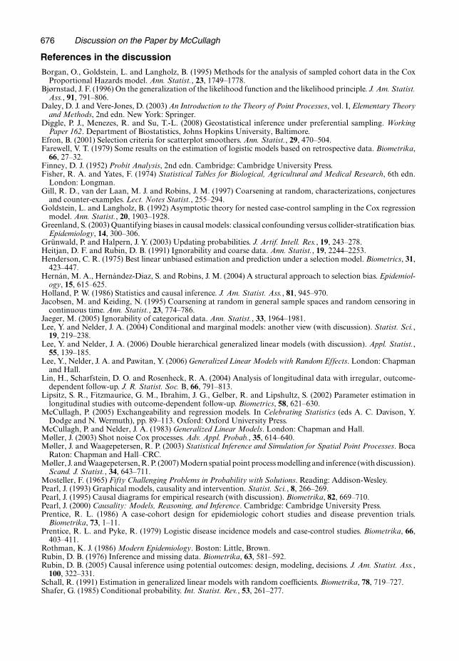
676 Discussion on the Paper by McCullagh
References in the discussion
Borgan, O., Goldstein, L. and Langholz, B. (1995) Methods for the analysis of sampled cohort data in the CoxProportional Hazards model. Ann. Statist., 23, 1749–1778.
Bjørnstad, J. F. (1996) On the generalization of the likelihood function and the likelihood principle. J. Am. Statist.Ass., 91, 791–806.
Daley, D. J. and Vere-Jones, D. (2003) An Introduction to the Theory of Point Processes, vol. I, Elementary Theoryand Methods, 2nd edn. New York: Springer.
Diggle, P. J., Menezes, R. and Su, T.-L. (2008) Geostatistical inference under preferential sampling. WorkingPaper 162. Department of Biostatistics, Johns Hopkins University, Baltimore.
Efron, B. (2001) Selection criteria for scatterplot smoothers. Ann. Statist., 29, 470–504.Farewell, V. T. (1979) Some results on the estimation of logistic models based on retrospective data. Biometrika,
66, 27–32.Finney, D. J. (1952) Probit Analysis, 2nd edn. Cambridge: Cambridge University Press.Fisher, R. A. and Yates, F. (1974) Statistical Tables for Biological, Agricultural and Medical Research, 6th edn.
London: Longman.Gill, R. D., van der Laan, M. J. and Robins, J. M. (1997) Coarsening at random, characterizations, conjectures
and counter-examples. Lect. Notes Statist., 255–294.Goldstein, L. and Langholz, B. (1992) Asymptotic theory for nested case-control sampling in the Cox regression
model. Ann. Statist., 20, 1903–1928.Greenland, S. (2003) Quantifying biases in causal models: classical confounding versus collider-stratification bias.
Epidemiology, 14, 300–306.Grünwald, P. and Halpern, J. Y. (2003) Updating probabilities. J. Artif. Intell. Res., 19, 243–278.Heitjan, D. F. and Rubin, D. B. (1991) Ignorability and coarse data. Ann. Statist., 19, 2244–2253.Henderson, C. R. (1975) Best linear unbiased estimation and prediction under a selection model. Biometrics, 31,
423–447.Hernán, M. A., Hernández-Diaz, S. and Robins, J. M. (2004) A structural approach to selection bias. Epidemiol-
ogy, 15, 615–625.Holland, P. W. (1986) Statistics and causal inference. J. Am. Statist. Ass., 81, 945–970.Jacobsen, M. and Keiding, N. (1995) Coarsening at random in general sample spaces and random censoring in
continuous time. Ann. Statist., 23, 774–786.Jaeger, M. (2005) Ignorability of categorical data. Ann. Statist., 33, 1964–1981.Lee, Y. and Nelder, J. A. (2004) Conditional and marginal models: another view (with discussion). Statist. Sci.,
19, 219–238.Lee, Y. and Nelder, J. A. (2006) Double hierarchical generalized linear models (with discussion). Appl. Statist.,
55, 139–185.Lee, Y., Nelder, J. A. and Pawitan, Y. (2006) Generalized Linear Models with Random Effects. London: Chapman
and Hall.Lin, H., Scharfstein, D. O. and Rosenheck, R. A. (2004) Analysis of longitudinal data with irregular, outcome-
dependent follow-up. J. R. Statist. Soc. B, 66, 791–813.Lipsitz, S. R., Fitzmaurice, G. M., Ibrahim, J. G., Gelber, R. and Lipshultz, S. (2002) Parameter estimation in
longitudinal studies with outcome-dependent follow-up. Biometrics, 58, 621–630.McCullagh, P. (2005) Exchangeability and regression models. In Celebrating Statistics (eds A. C. Davison, Y.
Dodge and N. Wermuth), pp. 89–113. Oxford: Oxford University Press.McCullagh, P. and Nelder, J. A. (1983) Generalized Linear Models. London: Chapman and Hall.Møller, J. (2003) Shot noise Cox processes. Adv. Appl. Probab., 35, 614–640.Møller, J. and Waagepetersen, R. P. (2003) Statistical Inference and Simulation for Spatial Point Processes. Boca
Raton: Chapman and Hall–CRC.Møller, J. and Waagepetersen, R. P. (2007) Modern spatial point process modelling and inference (with discussion).
Scand. J. Statist., 34, 643–711.Mosteller, F. (1965) Fifty Challenging Problems in Probability with Solutions. Reading: Addison-Wesley.Pearl, J. (1993) Graphical models, causality and intervention. Statist. Sci., 8, 266–269.Pearl, J. (1995) Causal diagrams for empirical research (with discussion). Biometrika, 82, 669–710.Pearl, J. (2000) Causality: Models, Reasoning, and Inference. Cambridge: Cambridge University Press.Prentice, R. L. (1986) A case-cohort design for epidemiologic cohort studies and disease prevention trials.
Biometrika, 73, 1–11.Prentice, R. L. and Pyke, R. (1979) Logistic disease incidence models and case-control studies. Biometrika, 66,
403–411.Rothman, K. J. (1986) Modern Epidemiology. Boston: Little, Brown.Rubin, D. B. (1976) Inference and missing data. Biometrika, 63, 581–592.Rubin, D. B. (2005) Causal inference using potential outcomes: design, modeling, decisions. J. Am. Statist. Ass.,
100, 322–331.Schall, R. (1991) Estimation in generalized linear models with random coefficients. Biometrika, 78, 719–727.Shafer, G. (1985) Conditional probability. Int. Statist. Rev., 53, 261–277.

Discussion on the Paper by McCullagh 677
Spirtes, P., Glymour, C. and Scheines, R. (1993) Causation, Prediction and Search. New York: Springer.Stiratelli, R., Laird, N. M. and Ware, J. (1984) Random-effects statistical model for serial observations with binary
response. Biometrics, 40, 961–971.Sun, J., Sun, L. and Liu, D. (2007) Regression analysis of longitudinal data in the presence of informative obser-
vation and censoring times. J. Am. Statist. Ass., 102, 1397–1406.Wahba, G. (1985) A comparison of GCV and GML for choosing the smoothing parameter in the generalized
spline smoothing problem. Ann. Statist., 13, 1378–1402.Wahba, G. (1990) Spline Models for Observational Data. Philadelphia: Society for Industrial and Applied Math-
ematics.Wilsdon, B. H. (1934) Discrimination by specification statistically considered and illustrated by the standard
specification for Portland cement (with discussion). J. R. Statist. Soc., suppl., 1, 152–206.