Sampling Archimedean copulas - hu-berlin.de · 2013-07-11 · power nested Archimedean copula based...

Sampling Archimedean copulas

Marius Hofert

[email protected]

Ulm University

2007-12-08

mailto:[email protected]


Outline

1 Nonnested Archimedean copulas

1.1 Marshall and Olkin’s algorithm

2 Nested Archimedean copulas

2.1 McNeil’s algorithm

2.2 A general nesting result

2.3 Special nesting results

2.4 Simulation results

2


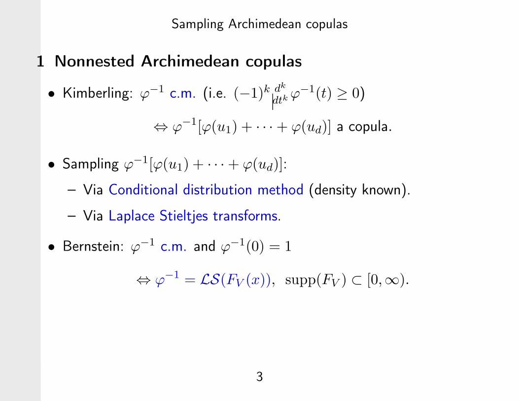
1 Nonnested Archimedean copulas

• Kimberling: ϕ−1 c.m. (i.e. (−1)k dk

dtkϕ−1(t) ≥ 0)

⇔ ϕ−1[ϕ(u1) + · · · + ϕ(ud)] a copula.

• Sampling ϕ−1[ϕ(u1) + · · · + ϕ(ud)]:

– Via Conditional distribution method (density known).

– Via Laplace Stieltjes transforms.

• Bernstein: ϕ−1 c.m. and ϕ−1(0) = 1

⇔ ϕ−1 = LS(FV (x)), supp(FV ) ⊂ [0,∞).

3


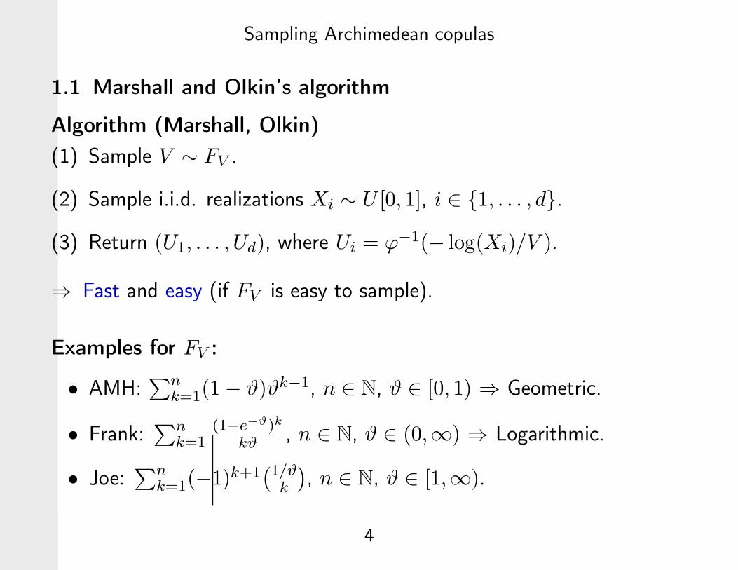
1.1 Marshall and Olkin’s algorithm

Algorithm (Marshall, Olkin)

(1) Sample V ∼ FV .

(2) Sample i.i.d. realizations Xi ∼ U [0, 1], i ∈ {1, . . . , d}.

(3) Return (U1, . . . , Ud), where Ui = ϕ−1(− log(Xi)/V ).

⇒ Fast and easy (if FV is easy to sample).

Examples for FV :

• AMH:∑n

k=1(1 − ϑ)ϑk−1, n ∈ N, ϑ ∈ [0, 1) ⇒ Geometric.

• Frank:∑n

k=1(1−e−ϑ)k

kϑ , n ∈ N, ϑ ∈ (0,∞) ⇒ Logarithmic.

• Joe:∑n

k=1(−1)k+1(1/ϑ

k

)

, n ∈ N, ϑ ∈ [1,∞).

4


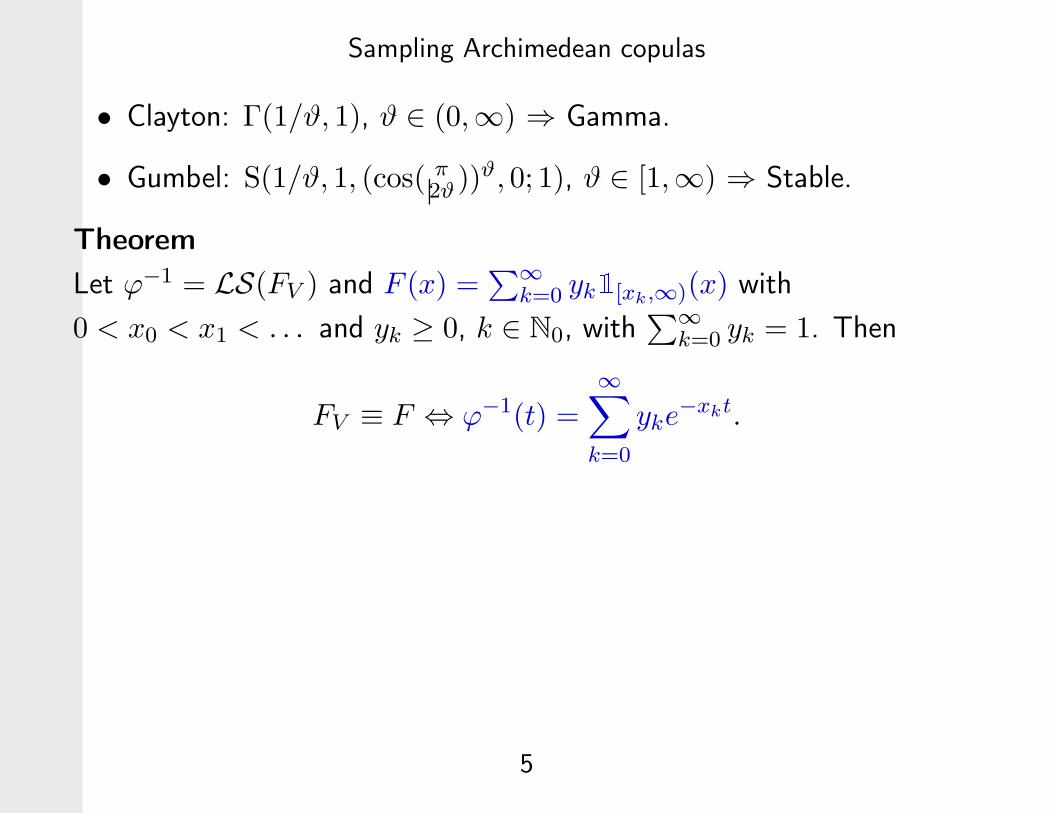
• Clayton: Γ(1/ϑ, 1), ϑ ∈ (0,∞) ⇒ Gamma.

• Gumbel: S(1/ϑ, 1, (cos( π2ϑ))ϑ, 0; 1), ϑ ∈ [1,∞) ⇒ Stable.

Theorem

Let ϕ−1 = LS(FV ) and F (x) =∑

∞

k=0 yk1[xk,∞)(x) with

0 < x0 < x1 < . . . and yk ≥ 0, k ∈ N0, with∑

∞

k=0 yk = 1. Then

FV ≡ F ⇔ ϕ−1(t) =∞

∑

k=0

yke−xkt.

5


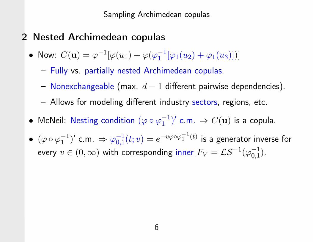
2 Nested Archimedean copulas

• Now: C(u) = ϕ−1[ϕ(u1) + ϕ(ϕ−11 [ϕ1(u2) + ϕ1(u3)])]

– Fully vs. partially nested Archimedean copulas.

– Nonexchangeable (max. d − 1 different pairwise dependencies).

– Allows for modeling different industry sectors, regions, etc.

• McNeil: Nesting condition (ϕ ◦ ϕ−11 )′ c.m. ⇒ C(u) is a copula.

• (ϕ ◦ϕ−11 )′ c.m. ⇒ ϕ−1

0,1(t; v) = e−vϕ◦ϕ−1

1(t) is a generator inverse for

every v ∈ (0,∞) with corresponding inner FV = LS−1(ϕ−10,1).

6


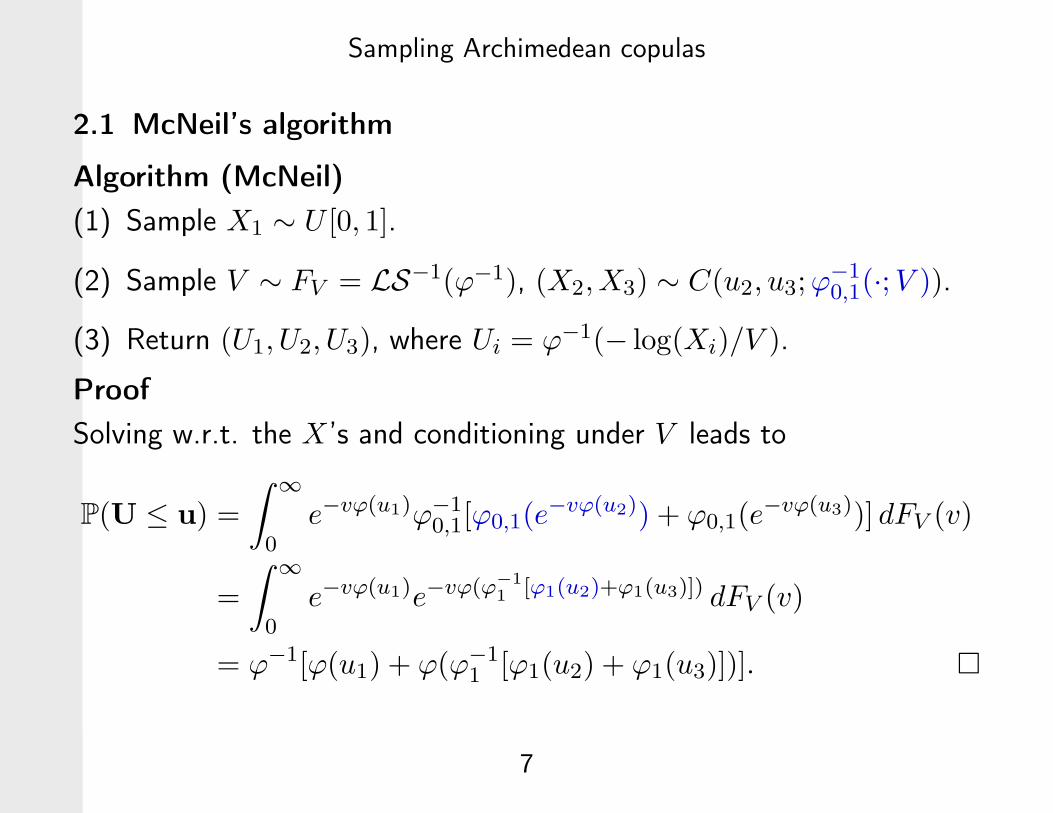
2.1 McNeil’s algorithm

Algorithm (McNeil)

(1) Sample X1 ∼ U [0, 1].

(2) Sample V ∼ FV = LS−1(ϕ−1), (X2,X3) ∼ C(u2, u3;ϕ−10,1(·;V )).

(3) Return (U1, U2, U3), where Ui = ϕ−1(− log(Xi)/V ).

Proof

Solving w.r.t. the X’s and conditioning under V leads to

P(U ≤ u) =

∫

∞

0e−vϕ(u1)ϕ−1

0,1[ϕ0,1(e−vϕ(u2)) + ϕ0,1(e

−vϕ(u3))] dFV (v)

=

∫

∞

0e−vϕ(u1)e−vϕ(ϕ−1

1[ϕ1(u2)+ϕ1(u3)]) dFV (v)

= ϕ−1[ϕ(u1) + ϕ(ϕ−11 [ϕ1(u2) + ϕ1(u3)])]. �

7


Examples:

• Nested Gumbel copula:

– ϕ−10,1(t; v) = e−vtϑ/ϑ1 ⇒ ϕ−1

0,1(t/c; v) with c = vϑ1/ϑ belongs to

the Gumbel family again.

– Sample C(u2, u3;ϕ−10,1(·/c;V )) (involves Stable distribution).

• Nested Clayton copula:

– ϕ−10,1(t; v) = e−v((1+t)ϑ/ϑ1−1) ⇒ Rejection algorithm (only for

large enough ϑ).

Questions:

• Which (classes of) generators can be used to build a nested

structure?

8


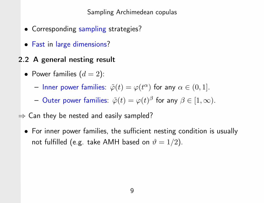
• Corresponding sampling strategies?

• Fast in large dimensions?

2.2 A general nesting result

• Power families (d = 2):

– Inner power families: ϕ(t) = ϕ(tα) for any α ∈ (0, 1].

– Outer power families: ϕ(t) = ϕ(t)β for any β ∈ [1,∞).

⇒ Can they be nested and easily sampled?

• For inner power families, the sufficient nesting condition is usually

not fulfilled (e.g. take AMH based on ϑ = 1/2).

9


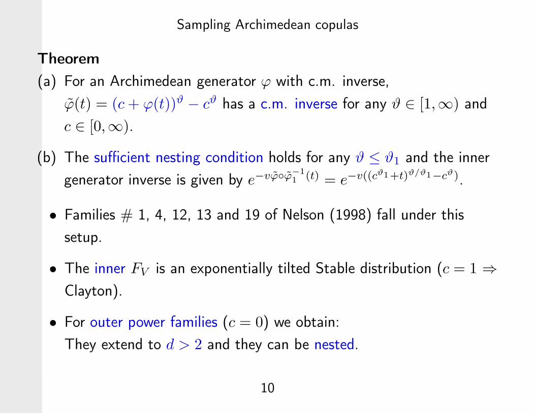
Theorem

(a) For an Archimedean generator ϕ with c.m. inverse,

ϕ(t) = (c + ϕ(t))ϑ − cϑ has a c.m. inverse for any ϑ ∈ [1,∞) and

c ∈ [0,∞).

(b) The sufficient nesting condition holds for any ϑ ≤ ϑ1 and the inner

generator inverse is given by e−vϕ◦ϕ−1

1(t) = e−v((cϑ1+t)ϑ/ϑ1−cϑ).

• Families # 1, 4, 12, 13 and 19 of Nelson (1998) fall under this

setup.

• The inner FV is an exponentially tilted Stable distribution (c = 1 ⇒

Clayton).

• For outer power families (c = 0) we obtain:

They extend to d > 2 and they can be nested.

10


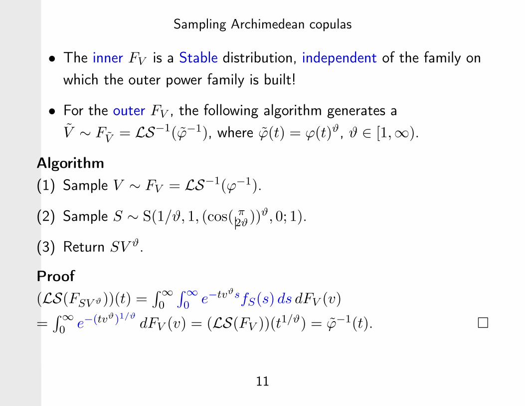
• The inner FV is a Stable distribution, independent of the family on

which the outer power family is built!

• For the outer FV , the following algorithm generates a

V ∼ FV = LS−1(ϕ−1), where ϕ(t) = ϕ(t)ϑ, ϑ ∈ [1,∞).

Algorithm

(1) Sample V ∼ FV = LS−1(ϕ−1).

(2) Sample S ∼ S(1/ϑ, 1, (cos( π2ϑ))ϑ, 0; 1).

(3) Return SV ϑ.

Proof

(LS(FSV ϑ))(t) =∫

∞

0

∫

∞

0 e−tvϑsfS(s) ds dFV (v)

=∫

∞

0 e−(tvϑ)1/ϑdFV (v) = (LS(FV ))(t1/ϑ) = ϕ−1(t). �

11


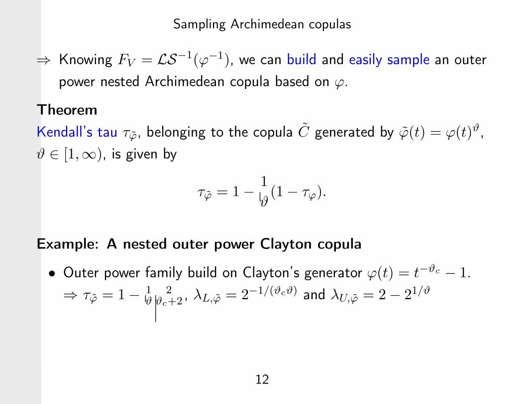
⇒ Knowing FV = LS−1(ϕ−1), we can build and easily sample an outer

power nested Archimedean copula based on ϕ.

Theorem

Kendall’s tau τϕ, belonging to the copula C generated by ϕ(t) = ϕ(t)ϑ,

ϑ ∈ [1,∞), is given by

τϕ = 1 −1

ϑ(1 − τϕ).

Example: A nested outer power Clayton copula

• Outer power family build on Clayton’s generator ϕ(t) = t−ϑc − 1.

⇒ τϕ = 1 − 1ϑ

2ϑc+2 , λL,ϕ = 2−1/(ϑcϑ) and λU,ϕ = 2 − 21/ϑ

12


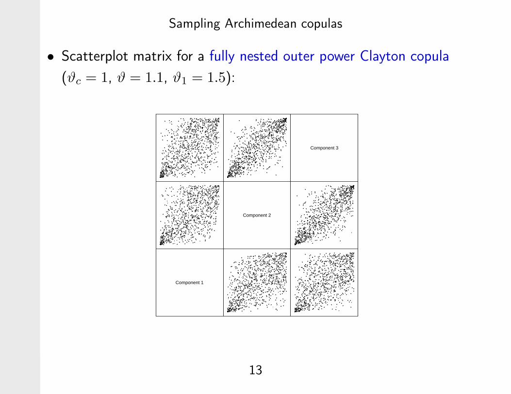
• Scatterplot matrix for a fully nested outer power Clayton copula

(ϑc = 1, ϑ = 1.1, ϑ1 = 1.5):

Component 1

Component 2

Component 3

13


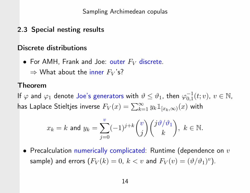
2.3 Special nesting results

Discrete distributions

• For AMH, Frank and Joe: outer FV discrete.

⇒ What about the inner FV ’s?

Theorem

If ϕ and ϕ1 denote Joe’s generators with ϑ ≤ ϑ1, then ϕ−10,1(t; v), v ∈ N,

has Laplace Stieltjes inverse FV (x) =∑

∞

k=1 yk1[xk,∞)(x) with

xk = k and yk =

v∑

j=0

(−1)j+k

(

v

j

)(

jϑ/ϑ1

k

)

, k ∈ N.

• Precalculation numerically complicated: Runtime (dependence on v

sample) and errors (FV (k) = 0, k < v and FV (v) = (ϑ/ϑ1)v).

14


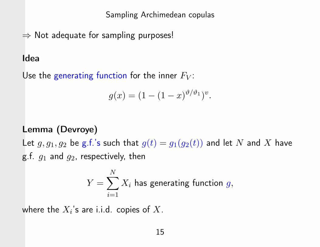
⇒ Not adequate for sampling purposes!

Idea

Use the generating function for the inner FV :

g(x) = (1 − (1 − x)ϑ/ϑ1)v.

Lemma (Devroye)

Let g, g1, g2 be g.f.’s such that g(t) = g1(g2(t)) and let N and X have

g.f. g1 and g2, respectively, then

Y =N

∑

i=1

Xi has generating function g,

where the Xi’s are i.i.d. copies of X.

15


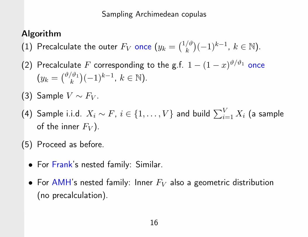
Algorithm

(1) Precalculate the outer FV once (yk =(1/ϑ

k

)

(−1)k−1, k ∈ N).

(2) Precalculate F corresponding to the g.f. 1 − (1 − x)ϑ/ϑ1 once

(yk =(ϑ/ϑ1

k

)

(−1)k−1, k ∈ N).

(3) Sample V ∼ FV .

(4) Sample i.i.d. Xi ∼ F , i ∈ {1, . . . , V } and build∑V

i=1 Xi (a sample

of the inner FV ).

(5) Proceed as before.

• For Frank’s nested family: Similar.

• For AMH’s nested family: Inner FV also a geometric distribution

(no precalculation).

16


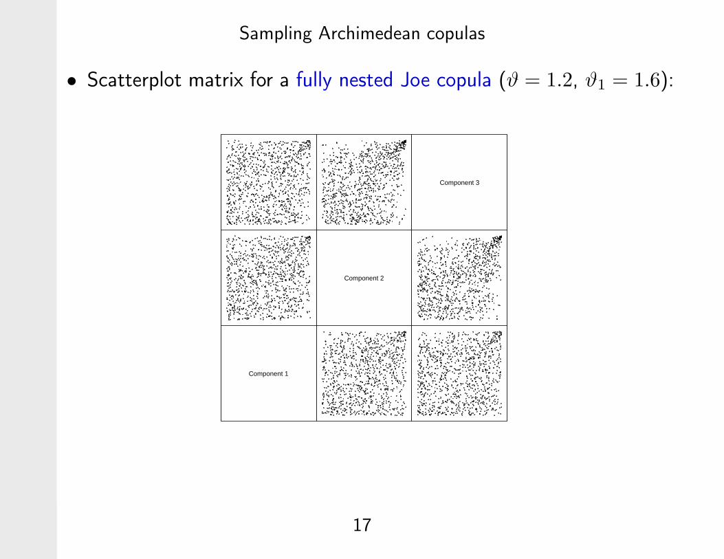
• Scatterplot matrix for a fully nested Joe copula (ϑ = 1.2, ϑ1 = 1.6):

Component 1

Component 2

Component 3

17


Mixed families

• Is it possible to mix different families?

• Examples from Nelson (1998): The sufficient nesting condition

holds for 7 family combinations including (AMH,Clayton) for

ϑ ∈ [0, 1), ϑ1 ∈ [1,∞).

A nested (AMH,Clayton) copula

• Parameters ϑ = 0.8 and ϑ1 = 2.

• Outer FV : Known geometric distribution.

• Inner FV : ϕ−10,1(t; v) = ((1 − ϑ)(1 + t)1/ϑ1 + ϑ)−v ⇒ Inner FV not

explicitly known.

18


Idea

Apply numerical inversion of Laplace transforms and numerical

rootfinding to obtain a realization from

FV (x) = (L−1(ϕ−1(t)/t))(x), x ∈ [0,∞).

• Methods:

– Fixed Talbot algorithm (contour deformation in the Bromwich

integral).

– Gaver Stehfest and Gaver Wynn rho algorithm (discrete analog

of the Post-Widder formula).

– Laguerre series algorithm (approximation via Laguerres series).

• Comparison in the known nonnested Clayton case (ϑ = 0.8):

19


Parameter calibration according to the precision requirement

maxx∈P

∣

∣

∣

FV (x) − FV (x)

FV (x)

∣

∣

∣< 0.0001 for P = {0.001, 0.002, . . . , 10}.

for an approximation FV to FV .

2.4 Simulation results

• χ2-test based on hypercubes of a partition into 5 parts for each

dimension.

• Maximal (MXDEV) and mean (MDEV) deviations of the

probabilities of falling in the hypercubes.

• Matrix of pairwise sample versions of Kendall’s tau.

• Visual check of plots of outer and inner FV ’s.

20


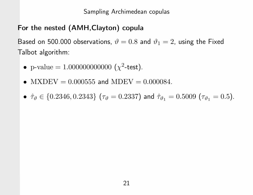
For the nested (AMH,Clayton) copula

Based on 500.000 observations, ϑ = 0.8 and ϑ1 = 2, using the Fixed

Talbot algorithm:

• p-value = 1.000000000000 (χ2-test).

• MXDEV = 0.000555 and MDEV = 0.000084.

• τϑ ∈ {0.2346, 0.2343} (τϑ = 0.2337) and τϑ1= 0.5009 (τϑ1

= 0.5).

21


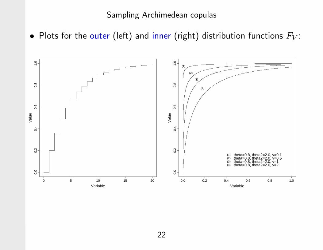
• Plots for the outer (left) and inner (right) distribution functions FV :

Variable

Val

ue0.

00.

20.

40.

60.

81.

0

0 5 10 15 20

Variable

Val

ue0.

00.

20.

40.

60.

81.

0

0.0 0.2 0.4 0.6 0.8 1.0

(1)

(2)

(3)

(4)

(1)(2)(3)(4)

theta=0.8, theta2=2.0, v=0.1theta=0.8, theta2=2.0, v=0.5theta=0.8, theta2=2.0, v=1theta=0.8, theta2=2.0, v=2

22


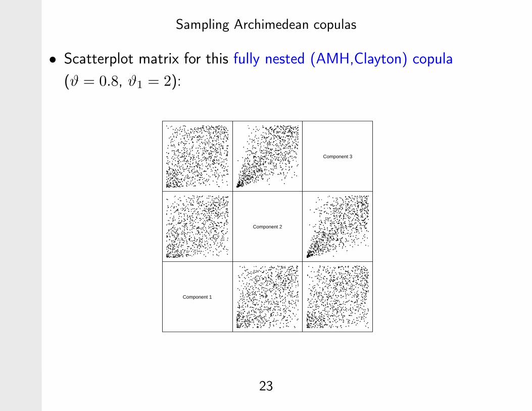
• Scatterplot matrix for this fully nested (AMH,Clayton) copula

(ϑ = 0.8, ϑ1 = 2):

Component 1

Component 2

Component 3

23


Runtimes

For 500.000 observations of ϕ−1[ϕ(u1) + ϕ(ϕ−11 [ϕ1(u2) + ϕ1(u3)])], we

obtain:

• (AMH,Clayton): 37.67s.

• Gumbel: 2.22s.

Outer power Clayton: 2.71s.

• Joe: 1.50s.

Frank: 1.60s.

AMH: 0.59s.

24

Sampling Archimedean copulas - hu-berlin.de · 2013-07-11 · power nested Archimedean copula based...

Documents

Transcript of Sampling Archimedean copulas - hu-berlin.de · 2013-07-11 · power nested Archimedean copula based...