
SAMPLE SOLUTIONS DIGITAL SIGNAL PROCESSING: · PDF file4 DIGITAL SIGNAL PROCESSING: Signals,...
25
SAMPLE SOLUTIONS DIGITAL SIGNAL PROCESSING: Signals, Systems, and Filters Andreas Antoniou (Revision date: February 7, 2007) SA.1 A periodic signal can be represented by the equation ˜ x(t)= 10 k=1 A k sin(ω k t + φ k ) where the frequencies ω k , amplitudes A k , and phase angles φ k are given in Table SA.1. The signal is to be processed first by an ideal bandpass filter and the by a differentiator, as shown in Fig. SA.1. The bandpass filter will pass frequencies in the range 4 ≤ ω ≤ 6 rad/s and reject all other frequencies and the differentiator will differentiate the signal with respect to time. (a) Obtain a time-domain representation for the signal at the outputs of the bandpass filter and differentiator, i.e., at nodes B and C, respectively, in Fig. SA.1. (b) Obtain a frequency-domain representation for the signal at the output of the bandpass filter. (c) Obtain a frequency-domain representation for the signal at the output of the differentiator. Bandpass Filter Differentiator B C A Figure SA.1 Table SA.1 Frequency Spectrum k ω k , rad/s A k φ k 1 1 0.3819 −0.3478 2 2 0.3614 0.8222 3 3 0.8575 2.3502 4 4 0.0629 −0.3292 5 5 0.1342 −0.1693 6 6 0.8648 0.6648 7 7 0.5155 −2.4473 8 8 0.6797 1.7780 9 9 0.7001 −1.5824 10 10 0.3 1.1 Copyright c by Andreas Antoniou 2005-
-
Upload
vuongxuyen -
Category
Documents
-
view
262 -
download
5
Transcript of SAMPLE SOLUTIONS DIGITAL SIGNAL PROCESSING: · PDF file4 DIGITAL SIGNAL PROCESSING: Signals,...
SAMPLE SOLUTIONS
DIGITAL SIGNAL PROCESSING: Signals, Systems, and Filters
Andreas Antoniou
(Revision date: February 7, 2007)
SA.1 A periodic signal can be represented by the equation
x̃(t) =10∑
k=1
Ak sin(ωkt + φk)
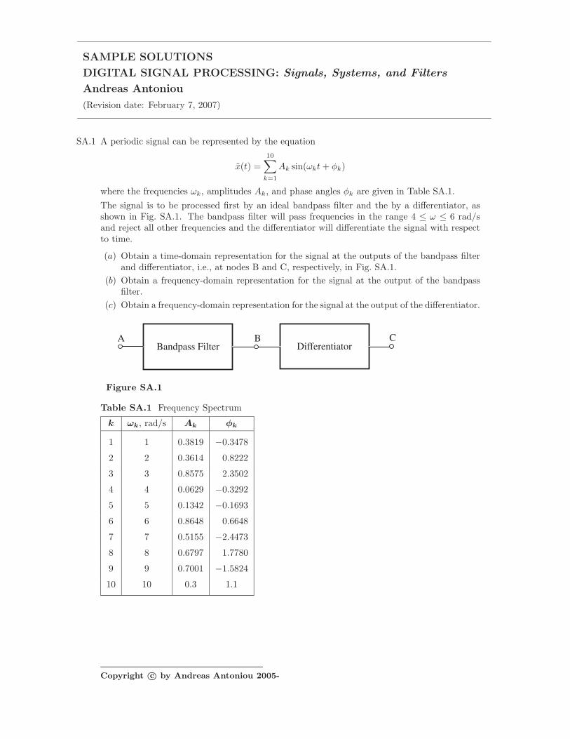
where the frequencies ωk, amplitudes Ak, and phase angles φk are given in Table SA.1.The signal is to be processed first by an ideal bandpass filter and the by a differentiator, asshown in Fig. SA.1. The bandpass filter will pass frequencies in the range 4 ≤ ω ≤ 6 rad/sand reject all other frequencies and the differentiator will differentiate the signal with respectto time.
(a) Obtain a time-domain representation for the signal at the outputs of the bandpass filterand differentiator, i.e., at nodes B and C, respectively, in Fig. SA.1.
(b) Obtain a frequency-domain representation for the signal at the output of the bandpassfilter.
(c) Obtain a frequency-domain representation for the signal at the output of the differentiator.
Bandpass Filter DifferentiatorB CA
Figure SA.1
Table SA.1 Frequency Spectrum
k ωk, rad/s Ak φk
1 1 0.3819 −0.3478
2 2 0.3614 0.8222
3 3 0.8575 2.3502
4 4 0.0629 −0.3292
5 5 0.1342 −0.1693
6 6 0.8648 0.6648
7 7 0.5155 −2.4473
8 8 0.6797 1.7780
9 9 0.7001 −1.5824
10 10 0.3 1.1
Copyright c© by Andreas Antoniou 2005-
2 DIGITAL SIGNAL PROCESSING: Signals, Systems, and Filters
Solution
(a) Node B:
xB(t) =6∑
k=4
Ak sin(ωkt + φk)
Node C:
xC(t) =d
dt
[6∑
k=4
Ak sin(ωkt + φk)
]=
6∑k=4
d
dt[Ak sin(ωkt + φk)]
=6∑
k=4
ωkAk cos(ωkt + φk) =6∑
k=4
ωkAk sin(ωkt + φk + π/2)
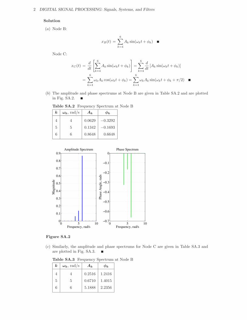
(b) The amplitude and phase spectrums at Node B are given in Table SA.2 and are plottedin Fig. SA.2.
Table SA.2 Frequency Spectrum at Node B
k ωk, rad/s Ak φk
4 4 0.0629 −0.3292
5 5 0.1342 −0.1693
6 6 0.8648 0.6648
0 5 100
0.1
0.2
0.3
0.4
0.5
0.6
0.7
0.8
0.9Amplitude Spectrum
Frequency, rad/s
Mag
nitu
de
0 5 10−0.7
−0.6
−0.5
−0.4
−0.3
−0.2
−0.1
0Phase Spectrum
Frequency, rad/s
Phas
e A
ngle
, rad
s
Figure SA.2
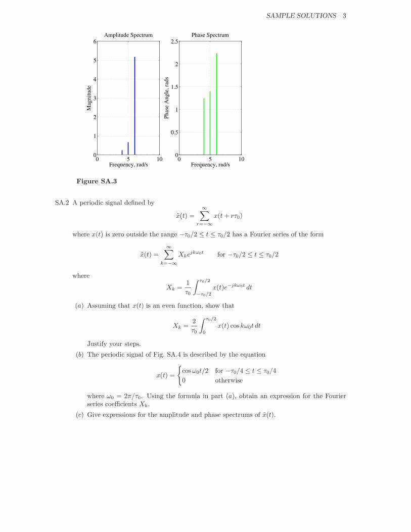
(c) Similarly, the amplitude and phase spectrums for Node C are given in Table SA.3 andare plotted in Fig. SA.3.
Table SA.3 Frequency Spectrum at Node B
k ωk, rad/s Ak φk
4 4 0.2516 1.2416
5 5 0.6710 1.4015
6 6 5.1888 2.2356
SAMPLE SOLUTIONS 3
0 5 100
1
2
3
4
5
6Amplitude Spectrum
Frequency, rad/s
Mag
nitu
de
0 5 100
0.5
1
1.5
2
2.5Phase Spectrum
Frequency, rad/sPh
ase
Ang
le, r
ads
Figure SA.3
SA.2 A periodic signal defined by
x̃(t) =∞∑
r=−∞x(t + rτ0)
where x(t) is zero outside the range −τ0/2 ≤ t ≤ τ0/2 has a Fourier series of the form
x̃(t) =∞∑
k=−∞Xkejkω0t for −τ0/2 ≤ t ≤ τ0/2
where
Xk =1τ0
∫ τ0/2
−τ0/2
x(t)e−jkω0t dt
(a) Assuming that x(t) is an even function, show that
Xk =2τ0
∫ τ0/2
0
x(t) cos kω0t dt
Justify your steps.
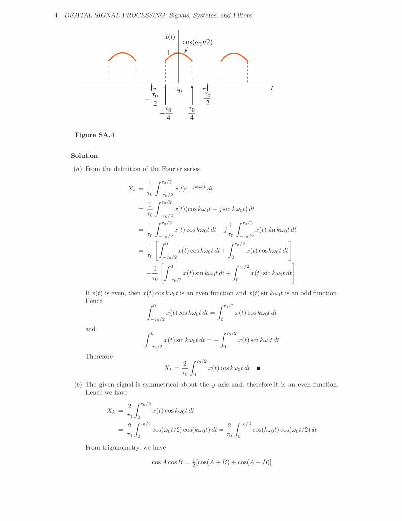
(b) The periodic signal of Fig. SA.4 is described by the equation
x(t) =
{cos ω0t/2 for −τ0/4 ≤ t ≤ τ0/40 otherwise
where ω0 = 2π/τ0. Using the formula in part (a), obtain an expression for the Fourierseries coefficients Xk.
(c) Give expressions for the amplitude and phase spectrums of x̃(t).
4 DIGITAL SIGNAL PROCESSING: Signals, Systems, and Filters
cos(ω0t/2)
t
x(t) ~
τ0
2 τ0
2 −
τ0
4 − τ0
4
τ0
Figure SA.4
Solution
(a) From the definition of the Fourier series
Xk =1τ0
∫ τ0/2
−τ0/2
x(t)e−jkω0t dt
=1τ0
∫ τ0/2
−τ0/2
x(t)(cos kω0t − j sin kω0t) dt
=1τ0
∫ τ0/2
−τ0/2
x(t) cos kω0t dt − j1τ0
∫ τ0/2
−τ0/2
x(t) sin kω0t dt
=1τ0
[∫ 0
−τ0/2
x(t) cos kω0t dt +∫ τ0/2
0
x(t) coskω0t dt
]
− 1τ0
[∫ 0
−τ0/2
x(t) sin kω0t dt +∫ τ0/2
0
x(t) sin kω0t dt
]
If x(t) is even, then x(t) coskω0t is an even function and x(t) sin kω0t is an odd function.Hence ∫ 0
−τ0/2
x(t) cos kω0t dt =∫ τ0/2
0
x(t) cos kω0t dt
and ∫ 0
−τ0/2
x(t) sin kω0t dt = −∫ τ0/2
0
x(t) sin kω0t dt
Therefore
Xk =2τ0
∫ τ0/2
0
x(t) coskω0t dt
(b) The given signal is symmetrical about the y axis and, therefore,it is an even function.Hence we have
Xk =2τ0
∫ τ0/2
0
x(t) cos kω0t dt
=2τ0
∫ τ0/4
0
cos(ω0t/2) cos(kω0t) dt =2τ0
∫ τ0/4
0
cos(kω0t) cos(ω0t/2) dt
From trigonometry, we have
cos A cos B = 12 [cos(A + B) + cos(A − B)]
SAMPLE SOLUTIONS 5
and, therefore,
Xk =2τ0
∫ τ0/4
0
12 [cos(kω0t + ω0t/2) + cos(kω0t − ω0t/2)] dt
=1τ0
∫ τ0/4
0
cos[(
k + 12
)ω0t]+ cos
[(k − 1
2
)ω0t]
dt
=1τ0
[sin[(
k + 12
)ω0t](
k + 12
)ω0
+sin[(
k − 12
)ω0t](
k − 12
)ω0
]τ0/4
0
=1τ0
⎡⎣sin
[(k + 1
2
)2πτ0
· τ04
](k + 1
2
)2πτ0
+sin[(
k − 12
)2πτ0
· τ04
](k − 1
2
)2πτ0
⎤⎦
=12π
[sin[(
k + 12
)π2
](k + 1
2
) +sin[(
k − 12
)π2
](k − 1
2
)]
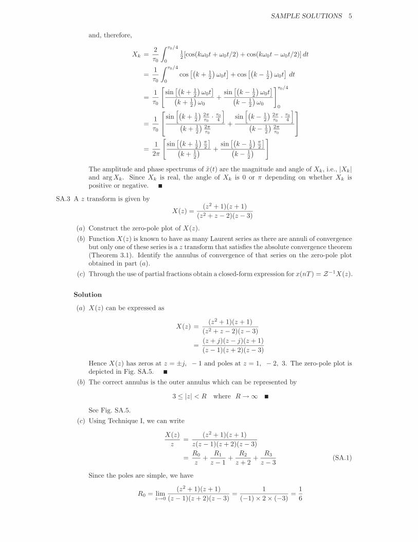
The amplitude and phase spectrums of x̃(t) are the magnitude and angle of Xk, i.e., |Xk|and arg Xk. Since Xk is real, the angle of Xk is 0 or π depending on whether Xk ispositive or negative.
SA.3 A z transform is given by
X(z) =(z2 + 1)(z + 1)
(z2 + z − 2)(z − 3)
(a) Construct the zero-pole plot of X(z).
(b) Function X(z) is known to have as many Laurent series as there are annuli of convergencebut only one of these series is a z transform that satisfies the absolute convergence theorem(Theorem 3.1). Identify the annulus of convergence of that series on the zero-pole plotobtained in part (a).
(c) Through the use of partial fractions obtain a closed-form expression for x(nT ) = Z−1X(z).
Solution
(a) X(z) can be expressed as
X(z) =(z2 + 1)(z + 1)
(z2 + z − 2)(z − 3)
=(z + j)(z − j)(z + 1)(z − 1)(z + 2)(z − 3)
Hence X(z) has zeros at z = ±j, − 1 and poles at z = 1, − 2, 3. The zero-pole plot isdepicted in Fig. SA.5.
(b) The correct annulus is the outer annulus which can be represented by
3 ≤ |z| < R where R → ∞See Fig. SA.5.
(c) Using Technique I, we can write
X(z)z
=(z2 + 1)(z + 1)
z(z − 1)(z + 2)(z − 3)
=R0
z+
R1
z − 1+
R2
z + 2+
R3
z − 3(SA.1)
Since the poles are simple, we have
R0 = limz→0
(z2 + 1)(z + 1)(z − 1)(z + 2)(z − 3)
=1
(−1) × 2 × (−3)=
16
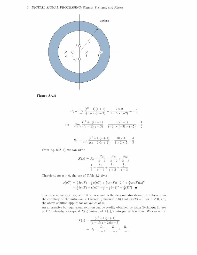
6 DIGITAL SIGNAL PROCESSING: Signals, Systems, and Filters
j
¡2 ¡1 1 3
R
¡j
z plane
Figure SA.5
R1 = limz→1
(z2 + 1)(z + 1)z(z + 2)(z − 3)
=2 × 2
1 × 3 × (−2)= −2
3
R2 = limz→−2
(z2 + 1)(z + 1)z(z − 1)(z − 3)
=5 × (−1)
(−2) × (−3) × (−5)=
16
R3 = limz→3
(z2 + 1)(z + 1)z(z − 1)(z + 2)
=10 × 4
3 × 2 × 5=
43
From Eq. (SA.1), we can write
X(z) = R0 +R1z
z − 1+
R2z
z + 2+
R3z
z − 3
=16−
23z
z − 1+
16z
z + 2+
43z
z − 3
Therefore, for n ≥ 0, the use of Table 3.2 gives
x(nT ) = 16δ(nT ) − 2
3u(nT ) + 16u(nT )(−2)n + 4
3u(nT )(3)n
= 16δ(nT ) + u(nT )[−2
3 + 16 (−2)n + 4
3 (3)n]
Since the numerator degree of X(z) is equal to the denominator degree, it follows fromthe corollary of the initial-value theorem (Theorem 3.8) that x(nT ) = 0 for n < 0, i.e.,the above solution applies for all values of n.An alternative but equivalent solution can be readily obtained by using Technique II (seep. 115) whereby we expand X(z) instead of X(z)/z into partial fractions. We can write
X(z) =(z2 + 1)(z + 1)
(z − 1)(z + 2)(z − 3)
= R0 +R1
z − 1+
R2
z + 2+
R3
z − 3
SAMPLE SOLUTIONS 7
where
R0 = limz→∞
(z2 + 1)(z + 1)(z − 1)(z + 2)(z − 3)
= limz→∞
z3
z3= 1
R1 = limz→1
(z2 + 1)(z + 1)(z + 2)(z − 3)
=2 × 2
3 × (−2)= −2
3
Thus
R2 = limz→−2
(z2 + 1)(z + 1)(z − 1)(z − 3)
=5 × (−1)
(−3) × (−5)= −1
3
R3 = limz→3
(z2 + 1)(z + 1)(z − 1)(z + 2)
=10 × 42 × 5
= 4
Thus
X(z) = 1 −23
z − 1−
13
z + 2+
4z − 3
and for n ≥ 0, we have
x(nT ) = δ(nT ) − 23u(nT − T ) − 1
3u(nT − T )(−2)n−1 + 4u(nT − T )(3)n−1
= δ(nT ) + u(nT − T )[−23 − 1
3 (−2)n−1 + 4(3)n−1]
SA.4 (a) Find the z transform of the following discrete-time signal
x(nT ) =
⎧⎪⎨⎪⎩
0 for n < 01 for 0 ≤ n ≤ 51 + (n − 5)T for n > 5
(b) The z transform of a discrete-time signal x(nT ) is given by
X(z) =z(3z2 − 2z + 1)(z2 + 1)(z − 1)
Using the initial-value theorem (Theorem 3.8), show that x(nT ) = 0 for n < 0. Thenfind x(nT ) for n ≥ 0 using the general inversion formula
x(nT ) =1
2πj
∮Γ
X(z)zn−1 dz.
Solution
(a) The signal can be expressed as
x(nT ) = u(nT ) + r(nT − 5T )
Hence
Zx(nT ) = Zu(nT ) + Zr(nT − 5T )= Zu(nT ) + z−5Zr(nT )
=z
z − 1− Tz−4
(z − 1)2
(a) The first nonzero value of x(nT ) occurs at KT = (N −M)T where N is the denominatordegree and M in the numerator degree in X(z). Since N = M = 3, we have K = 0, i.e.,the signal starts at KT = 0. Hence for n < 0, we have
x(nT ) = 0
8 DIGITAL SIGNAL PROCESSING: Signals, Systems, and Filters
(b) For n ≥ 0, we can write
x(nT ) =M∑i=1
Resz=pi
[X(z)zn−1
]
=M∑i=1
Resz=pi
z(3z2 − 2z + 1)zn−1
(z2 + 1)(z − 1)
=M∑i=1
Resz=pi
(3z2 − 2z + 1)zn
(z − j)(z + j)(z − 1)
=R1
z − j+
R∗1
z + j+
R2
z − 1(SA.2)
where M is the number of poles and R∗1 is the complex conjugate of R1 since the pole at
z = j = ejπ/2 is the complex conjugate of the pole at z = −j = e−jπ/2. Since the polesare simple, we have
R1 = limz→j
[(z − j)
(3z2 − 2z + 1)zn
(z − j)(z + j)(z − 1)
]
= limz→j
(3z2 − 2z + 1)zn
(z + j)(z − 1)=
(−3 − 2j + 1)jn
2j(j − 1)
=−2 − 2j
−2 − 2j= jn = ejnπ/2
and
R2 = limz→1
(3z2 − 2z + 1)zn
(z2 + 1)=
22
= 1
Therefore, from Eq. (SA.2), we can write
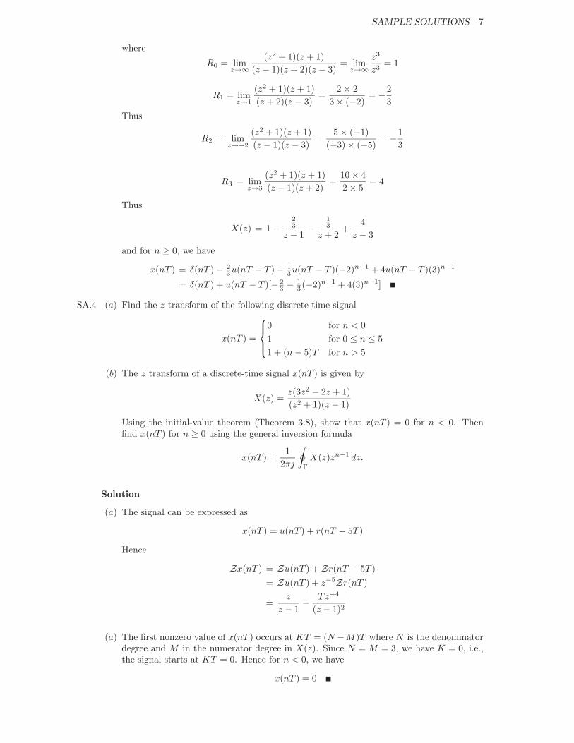
x(nT ) = u(nT )ejnπ/2 + u(nT )e−jnπ/2 + u(nT )= u(nT )(2 cosnπ/2 + 1)
SA.5 An initially relaxed discrete-time system can be represented by the equation
y(nT ) = Rx(nT ) = 2.5x(nT ) + |e0.1(nT+2T )|x(nT − T ) + x(nT − 2T )
By using appropriate tests, check the system for
(a) linearity,
(b) time invariance, and
(c) causality.
Solution
(a) Linearity
R[αx1(nT ) + βx2(nT )] = 2.5[αx1(nT ) + βx2(nT )] + |e0.1(nT+2T |[αx1(nT − T )+βx2(nT − T )] + [αx1(nT − 2T ) + βx2(nT − 2T )]
= α[2.5x1(nT ) + |e0.1(nT+2T )|x1(nT − T ) + x1(nT − 2T )]+β[2.5x2(nT ) + |e0.1(nT+2T )|x2(nT − T ) + x2(nT − 2T )]
= αRx1(nT ) + βRx2(nT )
Therefore, the system is linear.
SAMPLE SOLUTIONS 9
(b) Time invarianceThe response to a delayed excitation is
Rx(nT − kT ) = 2.5x(nT − kT ) + |e0.1(nT+2T )|x(nT − kT − T ) + x(nT − kT − 2T )
The delayed response is
y(nT − kT ) = 2.5x(nT − kT ) + |e0.1(nT−kT+2T )|x(nT − kT − T ) + x(nT − kT − 2T )
For any k �= 0, we have|e0.1nT+2T | �= |e0.1(nT−kT+2T )|
Thusy(nT − kT ) �= Rx(nT − kT )
and, therefore, the system is time dependent.
(c) Let x1(nT ) and x2(nT ) be arbitrary discrete-time signals such that
x1(nT ) = x2(nT ) for n ≤ k
x1(nT ) �= x2(nT ) for n > k
We have
Rx1(nT ) = 2.5x1(nT ) + |e0.1(nT+2T )|x1(nT − T ) + x1(nT − 2T ) (SA.3)
and
Rx2(nT ) = 2.5x2(nT ) + |e0.1(nT+2T )|x2(nT − T ) + x2(nT − 2T ) (SA.4)
Sincex1(nT ) = x2(nT ) for n ≤ k
thenx1(nT − T ) = x2(nT − T ) for n ≤ k
andx1(nT − 2T ) = x2(nT − 2T ) for n ≤ k
Hence the right-hand side in Eq. (SA.3) is equal to the right-hand side in Eq. (SA.4) forn ≤ k and thus
Rx1(nT ) = Rx2nT ) for n ≤ k
Therefore, the filter is causal.
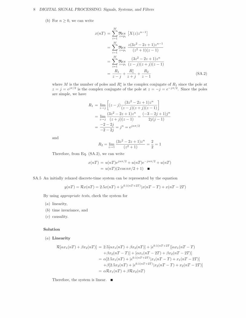
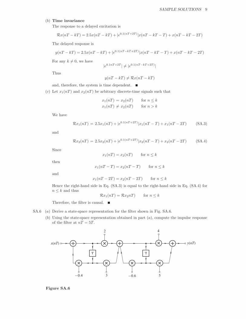
SA.6 (a) Derive a state-space representation for the filter shown in Fig. SA.6.
(b) Using the state-space representation obtained in part (a), compute the impulse responseof the filter at nT = 5T .
−0.4 −0.63
x(nT) y(nT)
2
5
4
Figure SA.6
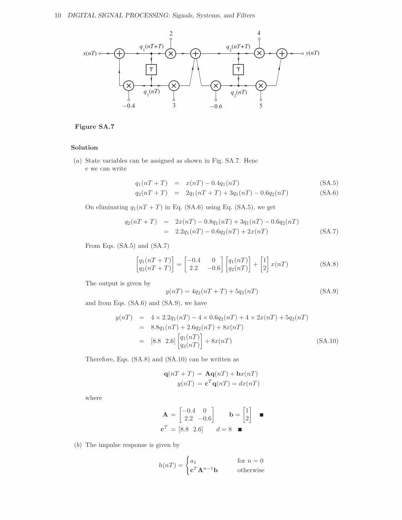
10 DIGITAL SIGNAL PROCESSING: Signals, Systems, and Filters
−0.4 −0.63
x(nT) y(nT)
2
5
4
q1(nT) q
2(nT)
q1(nT+T) q
2(nT+T)
Figure SA.7
Solution
(a) State variables can be assigned as shown in Fig. SA.7. Hence we can write
q1(nT + T ) = x(nT ) − 0.4q1(nT ) (SA.5)q2(nT + T ) = 2q1(nT + T ) + 3q1(nT ) − 0.6q2(nT ) (SA.6)
On eliminating q1(nT + T ) in Eq. (SA.6) using Eq. (SA.5), we get
q2(nT + T ) = 2x(nT ) − 0.8q1(nT ) + 3q1(nT ) − 0.6q2(nT )= 2.2q1(nT ) − 0.6q2(nT ) + 2x(nT ) (SA.7)
From Eqs. (SA.5) and (SA.7)[q1(nT + T )q2(nT + T )
]=[−0.4 0
2.2 −0.6
] [q1(nT )q2(nT )
]+[12
]x(nT ) (SA.8)
The output is given byy(nT ) = 4q2(nT + T ) + 5q2(nT ) (SA.9)
and from Eqs. (SA.6) and (SA.9), we have
y(nT ) = 4 × 2.2q1(nT ) − 4 × 0.6q2(nT ) + 4 × 2x(nT ) + 5q2(nT )= 8.8q1(nT ) + 2.6q2(nT ) + 8x(nT )
= [8.8 2.6][q1(nT )q2(nT )
]+ 8x(nT ) (SA.10)
Therefore, Eqs. (SA.8) and (SA.10) can be written as
q(nT + T ) = Aq(nT ) + bx(nT )y(nT ) = cT q(nT ) = dx(nT )
where
A =[−0.4 0
2.2 −0.6
]b =
[12
]cT = [8.8 2.6] d = 8
(b) The impulse response is given by
h(nT ) =
{a1 for n = 0cT An−1b otherwise
SAMPLE SOLUTIONS 11
For n = 5
h(5T ) = cT A4b = [8.8 2.6][−0.4 0
2.2 −0.6
]4 [12
]Since [−0.4 0
2.2 −0.6
]2
=[−0.4 0
2.2 −0.6
] [−0.4 02.2 −0.6
]=[
0.16 0.0−2.20 0.36
][−0.4 0
2.2 −0.6
]4
=[
0.16 0.0−2.20 0.36
] [0.16 0.0−2.20 0.36
]=[
0.0256 0.0−1.144 0.1296
]
we get
h(5T ) = [8.8 2.6][0.0256 0.0−1.144 0.1296
] [12
]= [8.8 2.6]
[0.0256−0.8848
]= −2.0752
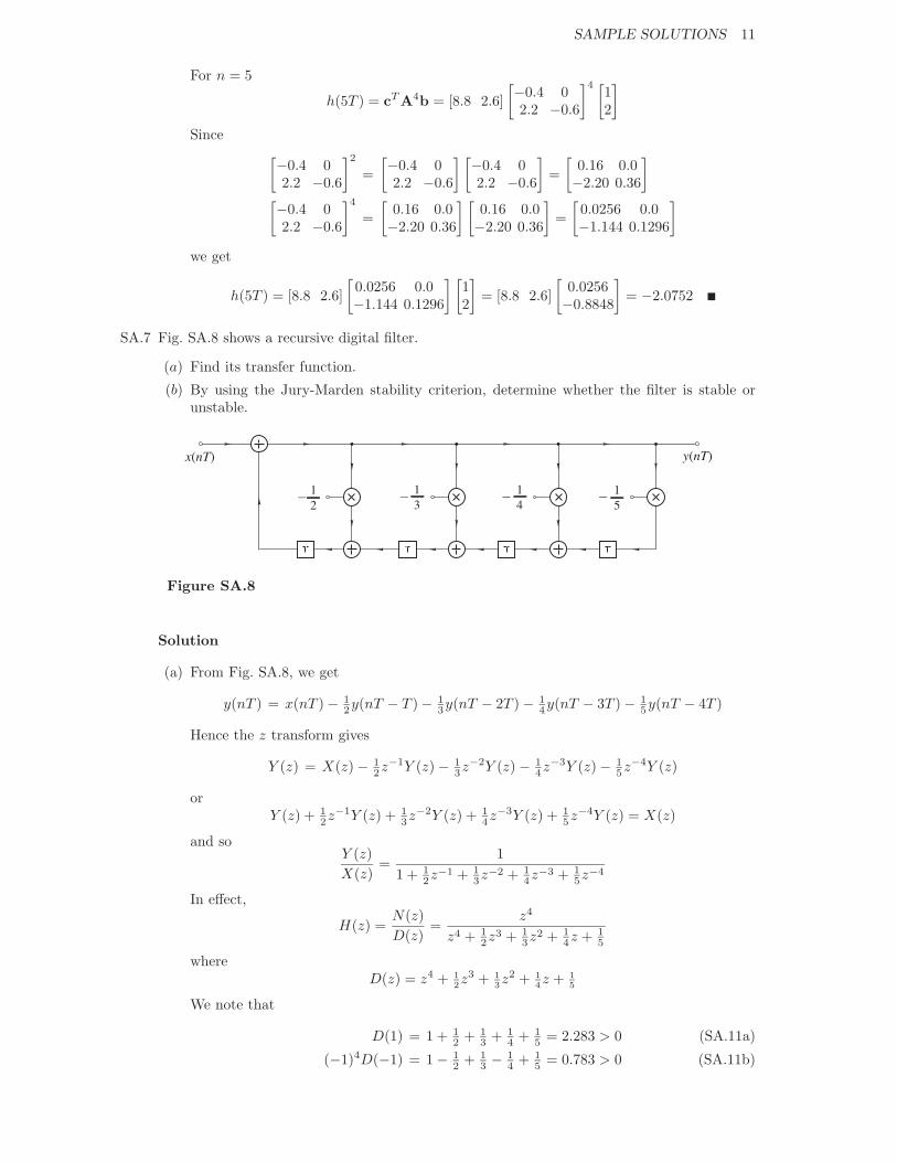
SA.7 Fig. SA.8 shows a recursive digital filter.
(a) Find its transfer function.
(b) By using the Jury-Marden stability criterion, determine whether the filter is stable orunstable.
x(nT) y(nT)
12
− 14
− 15
−13
−
Figure SA.8
Solution
(a) From Fig. SA.8, we get
y(nT ) = x(nT ) − 12y(nT − T ) − 1
3y(nT − 2T ) − 14y(nT − 3T ) − 1
5y(nT − 4T )
Hence the z transform gives
Y (z) = X(z) − 12z−1Y (z) − 1
3z−2Y (z) − 14z−3Y (z) − 1
5z−4Y (z)
orY (z) + 1
2z−1Y (z) + 13z−2Y (z) + 1
4z−3Y (z) + 15z−4Y (z) = X(z)
and soY (z)X(z)
=1
1 + 12z−1 + 1
3z−2 + 14z−3 + 1
5z−4
In effect,
H(z) =N(z)D(z)
=z4
z4 + 12z3 + 1
3z2 + 14z + 1
5
whereD(z) = z4 + 1
2z3 + 1
3z2 + 1
4z + 1
5
We note that
D(1) = 1 + 12 + 1
3 + 14 + 1
5 = 2.283 > 0 (SA.11a)
(−1)4D(−1) = 1 − 12 + 1
3 − 14 + 1
5 = 0.783 > 0 (SA.11b)
12 DIGITAL SIGNAL PROCESSING: Signals, Systems, and Filters
(b) The Jury-Marden array can be constructed as shown in Table SA.4.
Table SA.4 The Jury-Marden array
b0 b1 b2 b3 b4
1 1 12
13
14
15
2 15
14
13
12 1
3 2425
920
415
320
4 320
415
920
2425
5 0.8991 0.392 0.1885
From Eqs. (SA.11a) and (SA.11b) and Table SA.4, we have
D(1) > 0 (−1)4D(−1) > 0
b0 = 1 >15
= |b4|
|c0| =2425
>320
= |c3||d0| = 0.8991 > 0.1885 = |d2|
Therefore, conditions (i) to (iii) of the Jury-Marden stability criterion (see p. 220) aresatisfied and the filter is stable.
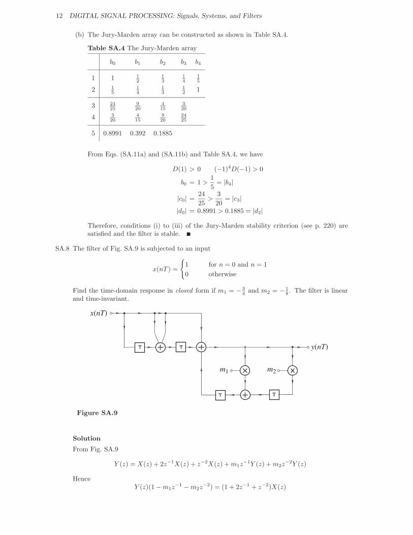
SA.8 The filter of Fig. SA.9 is subjected to an input
x(nT ) =
{1 for n = 0 and n = 10 otherwise
Find the time-domain response in closed form if m1 = −34 and m2 = −1
8 . The filter is linearand time-invariant.
x(nT)
m1 m2
y(nT)
Figure SA.9
Solution
From Fig. SA.9
Y (z) = X(z) + 2z−1X(z) + z−2X(z) + m1z−1Y (z) + m2z
−2Y (z)
HenceY (z)(1 − m1z
−1 − m2z−2) = (1 + 2z−1 + z−2)X(z)
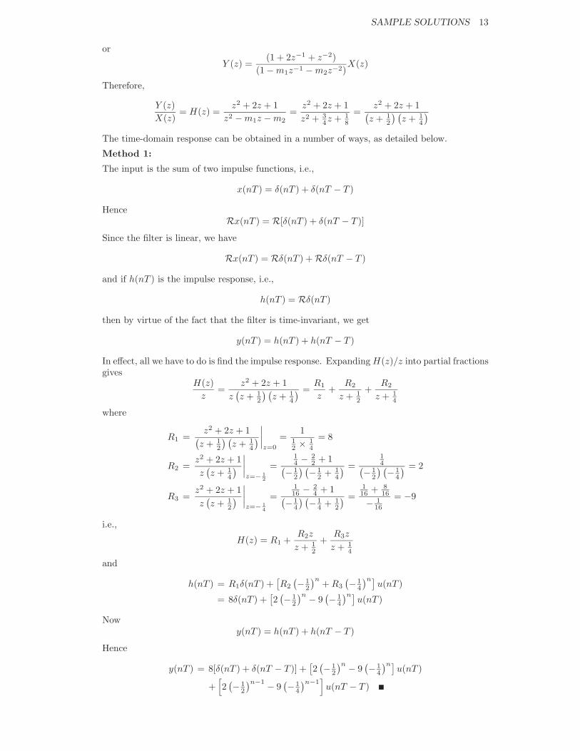
SAMPLE SOLUTIONS 13
or
Y (z) =(1 + 2z−1 + z−2)
(1 − m1z−1 − m2z−2)X(z)
Therefore,
Y (z)X(z)
= H(z) =z2 + 2z + 1
z2 − m1z − m2=
z2 + 2z + 1z2 + 3
4z + 18
=z2 + 2z + 1(
z + 12
) (z + 1
4
)The time-domain response can be obtained in a number of ways, as detailed below.
Method 1:
The input is the sum of two impulse functions, i.e.,
x(nT ) = δ(nT ) + δ(nT − T )
HenceRx(nT ) = R[δ(nT ) + δ(nT − T )]
Since the filter is linear, we have
Rx(nT ) = Rδ(nT ) + Rδ(nT − T )
and if h(nT ) is the impulse response, i.e.,
h(nT ) = Rδ(nT )
then by virtue of the fact that the filter is time-invariant, we get
y(nT ) = h(nT ) + h(nT − T )
In effect, all we have to do is find the impulse response. Expanding H(z)/z into partial fractionsgives
H(z)z
=z2 + 2z + 1
z(z + 1
2
) (z + 1
4
) =R1
z+
R2
z + 12
+R2
z + 14
where
R1 =z2 + 2z + 1(
z + 12
) (z + 1
4
) ∣∣∣∣z=0
=1
12 × 1
4
= 8
R2 =z2 + 2z + 1z(z + 1
4
) ∣∣∣∣z=− 1
2
=14 − 2
2 + 1(−12
) (−12 + 1
4
) =14(−1
2
) (−14
) = 2
R3 =z2 + 2z + 1z(z + 1
2
) ∣∣∣∣z=− 1
4
=116 − 2
4 + 1(−14
) (−14 + 1
2
) =116 + 8
16
− 116
= −9
i.e.,
H(z) = R1 +R2z
z + 12
+R3z
z + 14
and
h(nT ) = R1δ(nT ) +[R2
(−12
)n + R3
(−14
)n]u(nT )
= 8δ(nT ) +[2(−1
2
)n − 9(−1
4
)n]u(nT )
Nowy(nT ) = h(nT ) + h(nT − T )
Hence
y(nT ) = 8[δ(nT ) + δ(nT − T )] +[2(−1
2
)n − 9(−1
4
)n]u(nT )
+[2(−1
2
)n−1 − 9(−1
4
)n−1]u(nT − T )
14 DIGITAL SIGNAL PROCESSING: Signals, Systems, and Filters
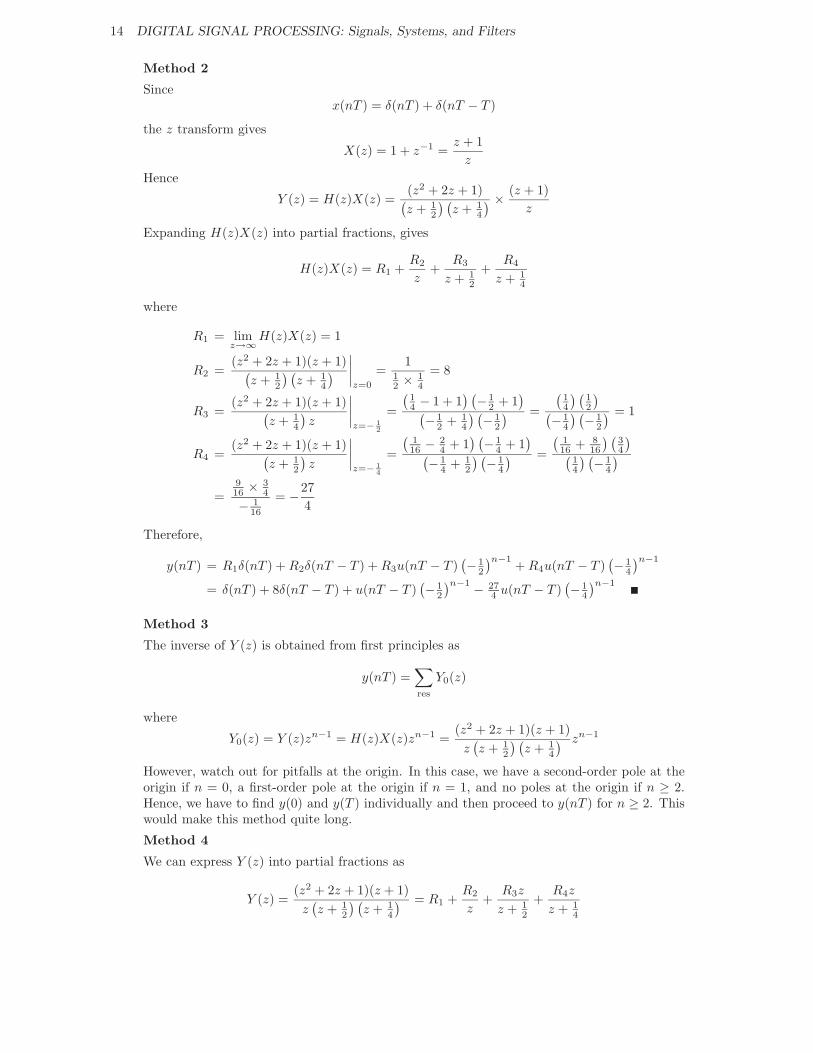
Method 2
Sincex(nT ) = δ(nT ) + δ(nT − T )
the z transform gives
X(z) = 1 + z−1 =z + 1
z
Hence
Y (z) = H(z)X(z) =(z2 + 2z + 1)(z + 1
2
) (z + 1
4
) × (z + 1)z
Expanding H(z)X(z) into partial fractions, gives
H(z)X(z) = R1 +R2
z+
R3
z + 12
+R4
z + 14
where
R1 = limz→∞H(z)X(z) = 1
R2 =(z2 + 2z + 1)(z + 1)(
z + 12
) (z + 1
4
) ∣∣∣∣z=0
=1
12 × 1
4
= 8
R3 =(z2 + 2z + 1)(z + 1)(
z + 14
)z
∣∣∣∣z=− 1
2
=
(14 − 1 + 1
) (−12 + 1
)(−12 + 1
4
) (−12
) =
(14
) (12
)(−14
) (−12
) = 1
R4 =(z2 + 2z + 1)(z + 1)(
z + 12
)z
∣∣∣∣z=− 1
4
=
(116 − 2
4 + 1) (−1
4 + 1)(−1
4 + 12
) (−14
) =
(116 + 8
16
) (34
)(14
) (−14
)=
916 × 3
4
− 116
= −274
Therefore,
y(nT ) = R1δ(nT ) + R2δ(nT − T ) + R3u(nT − T )(−1
2
)n−1 + R4u(nT − T )(−1
4
)n−1
= δ(nT ) + 8δ(nT − T ) + u(nT − T )(−1
2
)n−1 − 274 u(nT − T )
(−14
)n−1
Method 3
The inverse of Y (z) is obtained from first principles as
y(nT ) =∑res
Y0(z)
where
Y0(z) = Y (z)zn−1 = H(z)X(z)zn−1 =(z2 + 2z + 1)(z + 1)z(z + 1
2
) (z + 1
4
) zn−1
However, watch out for pitfalls at the origin. In this case, we have a second-order pole at theorigin if n = 0, a first-order pole at the origin if n = 1, and no poles at the origin if n ≥ 2.Hence, we have to find y(0) and y(T ) individually and then proceed to y(nT ) for n ≥ 2. Thiswould make this method quite long.
Method 4
We can express Y (z) into partial fractions as
Y (z) =(z2 + 2z + 1)(z + 1)z(z + 1
2
) (z + 1
4
) = R1 +R2
z+
R3z
z + 12
+R4z
z + 14
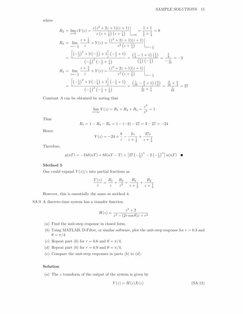
SAMPLE SOLUTIONS 15
where
R2 = limz=0
zY (z) =z(z2 + 2z + 1)(z + 1)
z(z + 1
2
) (z + 1
4
) ∣∣∣∣z=0
=1 × 112 × 1
4
= 8
R3 = limz=− 1
2
z + 12
z× Y (z) =
(z2 + 2z + 1)(z + 1)z2(z + 1
4
) ∣∣∣∣z=− 1
2
=
[(−12
)2 + 2(−1
2
)+ 1
] (−12 + 1
)(−1
2
)2 (−12 + 1
4
) =
(14 − 1 + 1
) (12
)(14
) (−14
) =18
− 116
= −2
R4 = limz=− 1
4
z + 14
z× Y (z) =
(z2 + 2z + 1)(z + 1)z2(z + 1
2
) ∣∣∣∣z=− 1
4
=
[(−14
)2 + 2(−1
4
)+ 1
] (−14 + 1
)(−1
4
)2 (−14 + 1
2
) =
(116 − 2
4 + 1) (
34
)116 × 1
4
=916 × 3
4164
= 27
Constant A can be obtained by noting that
limz=∞Y (z) = R1 + R3 + R4 =
z3
z3= 1
ThusR1 = 1 − R3 − R4 = 1 − (−2) − 27 = 3 − 27 = −24
HenceY (z) = −24 +
8z− 2z
z + 12
+27z
z + 14
Therefore,
y(nT ) = −24δ(nT ) + 8δ(nT − T ) +[27(−1
4
)n − 2(−1
2
)n]u(nT )
Method 5
One could expand Y (z)/z into partial fractions as
Y (z)z
=R1
z+
R2
z2+
R3
z + 12
+R4
z + 14
However, this is essentially the same as method 4.
SA.9 A discrete-time system has a transfer function
H(z) =z2 + 2
z2 − (2r cos θ)z + r2
(a) Find the unit-step response in closed form.
(b) Using MATLAB, D-Filter, or similar software, plot the unit-step response for r = 0.3 andθ = π/4.
(c) Repeat part (b) for r = 0.6 and θ = π/4.
(d) Repeat part (b) for r = 0.9 and θ = π/4.
(e) Compare the unit-step responses in parts (b) to (d).
Solution
(a) The z transform of the output of the system is given by
Y (z) = H(z)X(z) (SA.12)
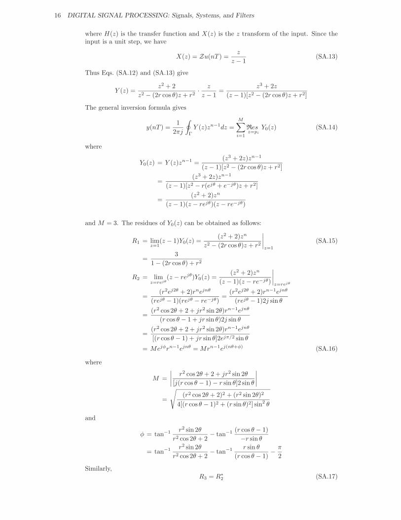
16 DIGITAL SIGNAL PROCESSING: Signals, Systems, and Filters
where H(z) is the transfer function and X(z) is the z transform of the input. Since theinput is a unit step, we have
X(z) = Zu(nT ) =z
z − 1(SA.13)
Thus Eqs. (SA.12) and (SA.13) give
Y (z) =z2 + 2
z2 − (2r cos θ)z + r2· z
z − 1=
z3 + 2z
(z − 1)[z2 − (2r cos θ)z + r2]
The general inversion formula gives
y(nT ) =1
2πj
∮Γ
Y (z)zn−1dz =M∑i=1
Resz=pi
Y0(z) (SA.14)
where
Y0(z) = Y (z)zn−1 =(z3 + 2z)zn−1
(z − 1)[z2 − (2r cos θ)z + r2]
=(z3 + 2z)zn−1
(z − 1)[z2 − r(ejθ + e−jθ)z + r2]
=(z2 + 2)zn
(z − 1)(z − rejθ)(z − re−jθ)
and M = 3. The residues of Y0(z) can be obtained as follows:
R1 = limz=1
(z − 1)Y0(z) =(z2 + 2)zn
z2 − (2r cos θ)z + r2
∣∣∣∣z=1
(SA.15)
=3
1 − (2r cos θ) + r2
R2 = limz=rejθ
(z − rejθ)Y0(z) =(z2 + 2)zn
(z − 1)(z − re−jθ)
∣∣∣∣z=rejθ
=(r2ej2θ + 2)rnejnθ
(rejθ − 1)(rejθ − re−jθ)=
(r2ej2θ + 2)rn−1ejnθ
(rejθ − 1)2j sin θ
=(r2 cos 2θ + 2 + jr2 sin 2θ)rn−1ejnθ
(r cos θ − 1 + jr sin θ)2j sin θ
=(r2 cos 2θ + 2 + jr2 sin 2θ)rn−1ejnθ
[(r cos θ − 1) + jr sin θ]2ejπ/2 sin θ
= Mejφrn−1ejnθ = Mrn−1ej(nθ+φ) (SA.16)
where
M =∣∣∣∣ r2 cos 2θ + 2 + jr2 sin 2θ
[j(r cos θ − 1) − r sin θ]2 sin θ
∣∣∣∣=
√(r2 cos 2θ + 2)2 + (r2 sin 2θ)2
4[(r cos θ − 1)2 + (r sin θ)2] sin2 θ
and
φ = tan−1 r2 sin 2θ
r2 cos 2θ + 2− tan−1 (r cos θ − 1)
−r sin θ
= tan−1 r2 sin 2θ
r2 cos 2θ + 2− tan−1 r sin θ
(r cos θ − 1)− π
2
Similarly,R3 = R∗
2 (SA.17)
SAMPLE SOLUTIONS 17
since complex conjugate poles give complex conjugate residues. We note that there is noadditional pole at the origin when n = 0 and hence for n ≥ 0 Eq. (SA.14) gives
y(nT ) = R1 + R2 + R∗2 (SA.18)
Since the numerator degree in Y (z) does not exceed the denominator degree, we have
y(nT ) = 0 for n < 0
Therefore, for any n, Eqs. (SA.15)–(SA.18) give
y(nT ) = u(nT )[R1 + Mrn−1ej(nθ+φ) + Mrn−1e−j(nθ+φ)
]= u(nT )
[R1 + 2Mrn−1 cos(nθ + φ)
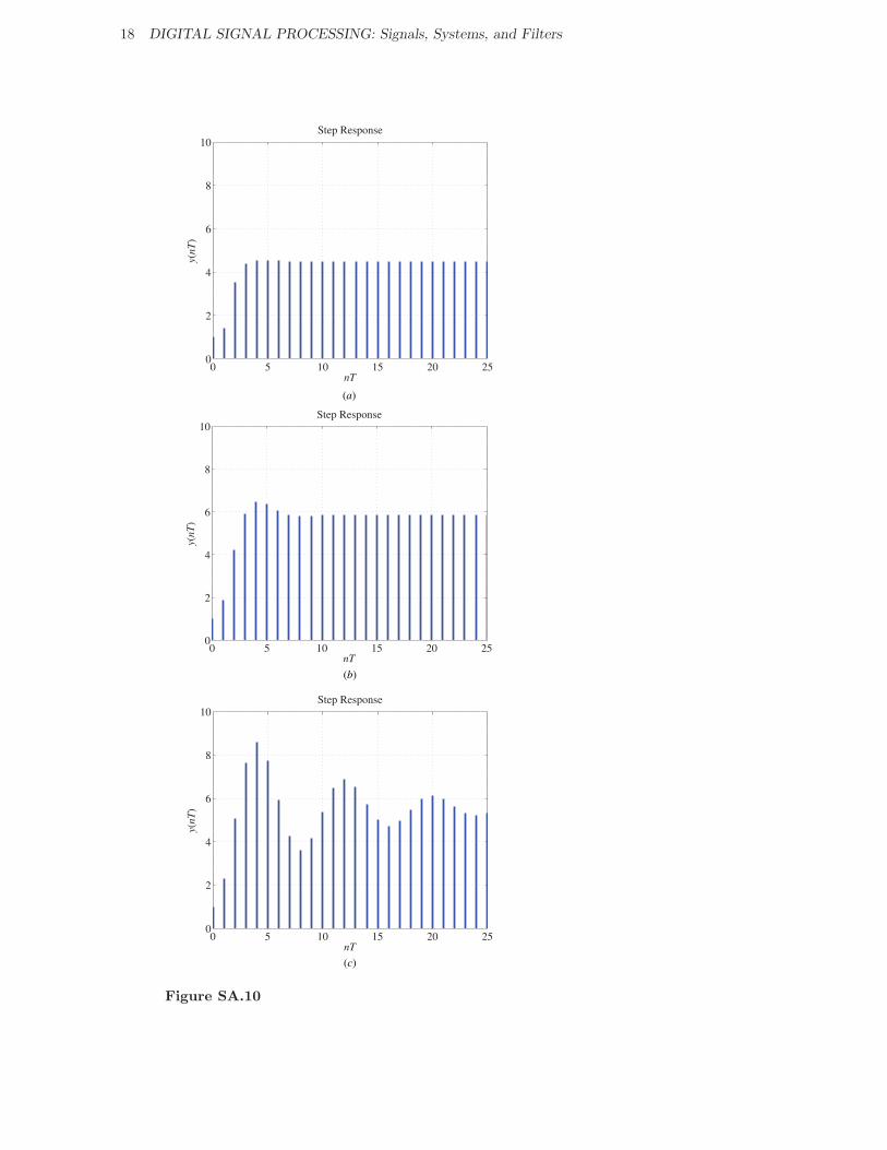
](b) and (d) The step responses for the three cases are illustrated in Fig. SA.10a to c.
(e) On the basis of the step responses obtained, the system in part (b) is what they calloverdamped, the one in part (c) is critically damped, and the one in part (d) is referred toas underdamped.
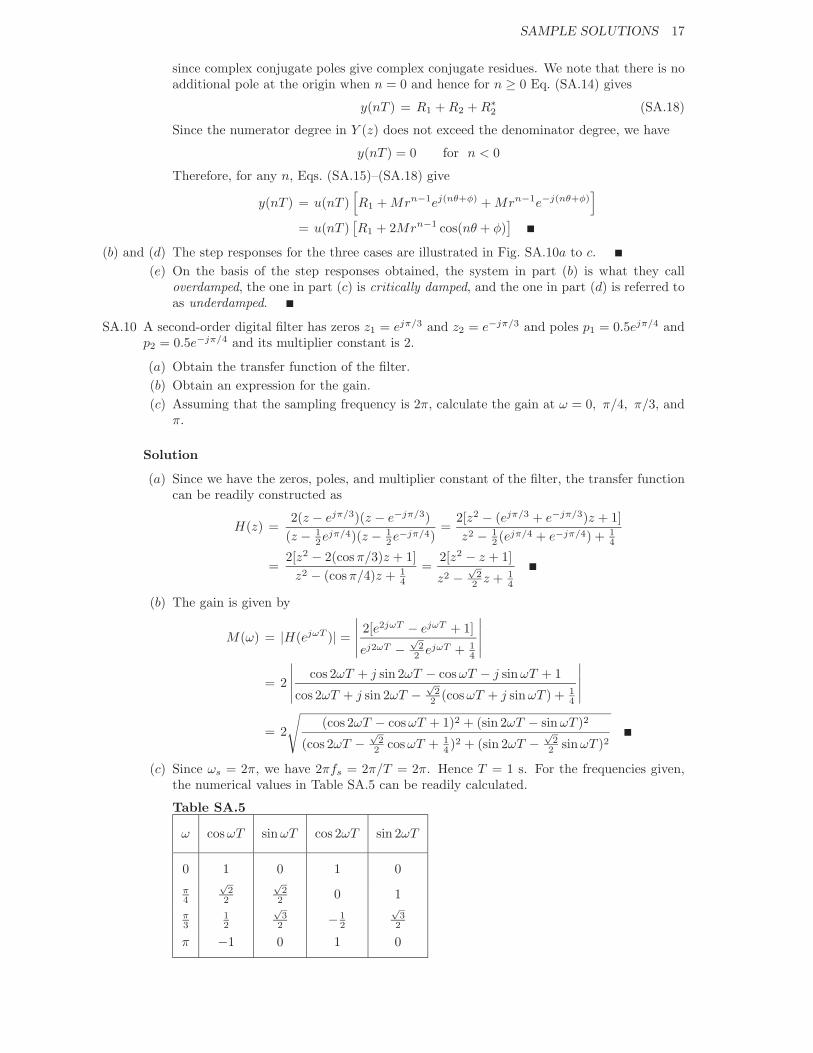
SA.10 A second-order digital filter has zeros z1 = ejπ/3 and z2 = e−jπ/3 and poles p1 = 0.5ejπ/4 andp2 = 0.5e−jπ/4 and its multiplier constant is 2.
(a) Obtain the transfer function of the filter.(b) Obtain an expression for the gain.(c) Assuming that the sampling frequency is 2π, calculate the gain at ω = 0, π/4, π/3, and
π.
Solution
(a) Since we have the zeros, poles, and multiplier constant of the filter, the transfer functioncan be readily constructed as
H(z) =2(z − ejπ/3)(z − e−jπ/3)
(z − 12ejπ/4)(z − 1
2e−jπ/4)=
2[z2 − (ejπ/3 + e−jπ/3)z + 1]z2 − 1
2 (ejπ/4 + e−jπ/4) + 14
=2[z2 − 2(cos π/3)z + 1]
z2 − (cosπ/4)z + 14
=2[z2 − z + 1]
z2 −√
22 z + 1
4
(b) The gain is given by
M(ω) = |H(ejωT )| =
∣∣∣∣∣ 2[e2jωT − ejωT + 1]
ej2ωT −√
22 ejωT + 1
4
∣∣∣∣∣= 2
∣∣∣∣∣ cos 2ωT + j sin 2ωT − cos ωT − j sin ωT + 1
cos 2ωT + j sin 2ωT −√
22 (cos ωT + j sin ωT ) + 1
4
∣∣∣∣∣= 2
√(cos 2ωT − cos ωT + 1)2 + (sin 2ωT − sin ωT )2
(cos 2ωT −√
22 cos ωT + 1
4 )2 + (sin 2ωT −√
22 sin ωT )2
(c) Since ωs = 2π, we have 2πfs = 2π/T = 2π. Hence T = 1 s. For the frequencies given,the numerical values in Table SA.5 can be readily calculated.
Table SA.5
ω cos ωT sin ωT cos 2ωT sin 2ωT
0 1 0 1 0π4
√2
2
√2
2 0 1π3
12
√3
2 −12
√3
2
π −1 0 1 0
18 DIGITAL SIGNAL PROCESSING: Signals, Systems, and Filters
0 5 10 15 20 250
2
4
6
8
10Step Response
nT
y(nT
)
0 5 10 15 20 250
2
4
6
8
10Step Response
nT
y(nT
)
0 5 10 15 20 250
2
4
6
8
10Step Response
nT
y(nT
)
(a)
(b)
(c)
Figure SA.10
SAMPLE SOLUTIONS 19
Thus
M(0) = 2
√(1 − 1 + 1)2 + (0 − 0)2
(1 −√
22 + 1
4 )2 + (0 − 0)2=
25−2
√2
4
= 3.6840
M(π
4
)= 2
√√√√ (0 −√
22 + 1)2 + (1 −
√2
2 )2
(0 −√
22 ×
√2
2 + 14 )2 + (1 −
√2
2 ×√
22 )2
= 2
√(2 −√
2)2 + (2 −√2)2
( 12 − 1)2 + 1
= 2
√2(2 −√
2)2
(−12 )2 + 1
= 1.489
M(π
3
)= 2
√√√√ (−12 − 1
2 + 1)2 + (√
32 −
√3
2 )2
(−12 −
√2
2 × 12 + 1
4 )2 + (√
32 −
√2
2 ×√
32 )
= 2
√√√√ 0 + 0(1−2−√
24
)2
+ · · ·= 0
M(π) = 2
√(1 + 1 + 1)2 + (0 − 0)
(1 +√
22 + 1
4 )2 + (0 − 0)= 2
√32 × 16
(4 + 2√
2 + 1)2
=2 × 3 × 4
4 + 2√
2 + 1= 3.0658
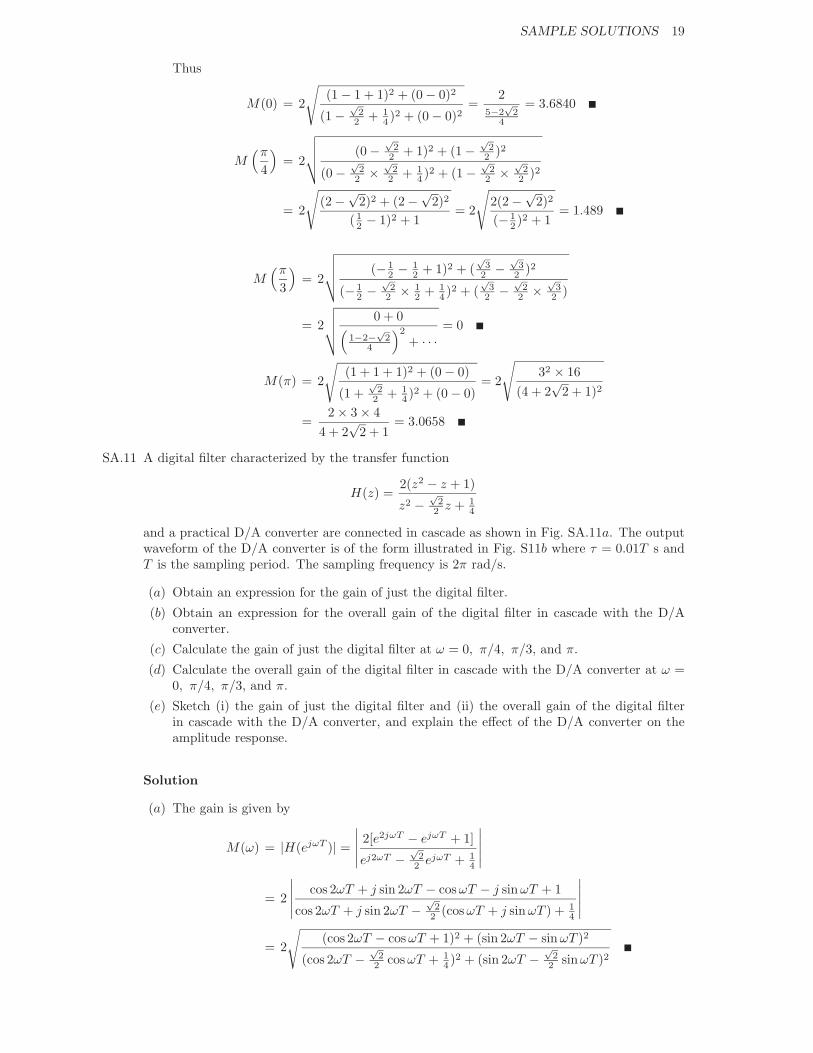
SA.11 A digital filter characterized by the transfer function
H(z) =2(z2 − z + 1)
z2 −√
22 z + 1
4
and a practical D/A converter are connected in cascade as shown in Fig. SA.11a. The outputwaveform of the D/A converter is of the form illustrated in Fig. S11b where τ = 0.01T s andT is the sampling period. The sampling frequency is 2π rad/s.
(a) Obtain an expression for the gain of just the digital filter.
(b) Obtain an expression for the overall gain of the digital filter in cascade with the D/Aconverter.
(c) Calculate the gain of just the digital filter at ω = 0, π/4, π/3, and π.
(d) Calculate the overall gain of the digital filter in cascade with the D/A converter at ω =0, π/4, π/3, and π.
(e) Sketch (i) the gain of just the digital filter and (ii) the overall gain of the digital filterin cascade with the D/A converter, and explain the effect of the D/A converter on theamplitude response.
Solution
(a) The gain is given by
M(ω) = |H(ejωT )| =
∣∣∣∣∣ 2[e2jωT − ejωT + 1]
ej2ωT −√
22 ejωT + 1
4
∣∣∣∣∣= 2
∣∣∣∣∣ cos 2ωT + j sin 2ωT − cos ωT − j sin ωT + 1
cos 2ωT + j sin 2ωT −√
22 (cos ωT + j sin ωT ) + 1
4
∣∣∣∣∣= 2
√(cos 2ωT − cos ωT + 1)2 + (sin 2ωT − sin ωT )2
(cos 2ωT −√
22 cos ωT + 1
4 )2 + (sin 2ωT −√
22 sin ωT )2
20 DIGITAL SIGNAL PROCESSING: Signals, Systems, and Filters
kT¿ t
y(kT)
(b)
DigitalFilter
y(t)˜
y(t)˜
x(nT)y(nT)
(a)
Practical D/A
converter
Figure SA.11
(b) The practical D/A converter has a gain
|Hp(jω)| = τ
∣∣∣∣ sin(ωτ/2)ωτ/2
∣∣∣∣ (SA.19)
where τ = 0.01T and T = 2π/ωs = 2π/2π = 1 s (see Eq. (6.60) in textbook). Hence theoverall gain of the digital filter in cascade with the D/A converter is given by
MT (ω) = 2
√(cos 2ωT − cos ωT + 1)2 + (sin 2ωT − sin ωT )2
(cos 2ωT −√
22 cos ωT + 1
4 )2 + (sin 2ωT −√
22 sin ωT )2
· τ∣∣∣∣ sin ωτ/2
ωτ/2
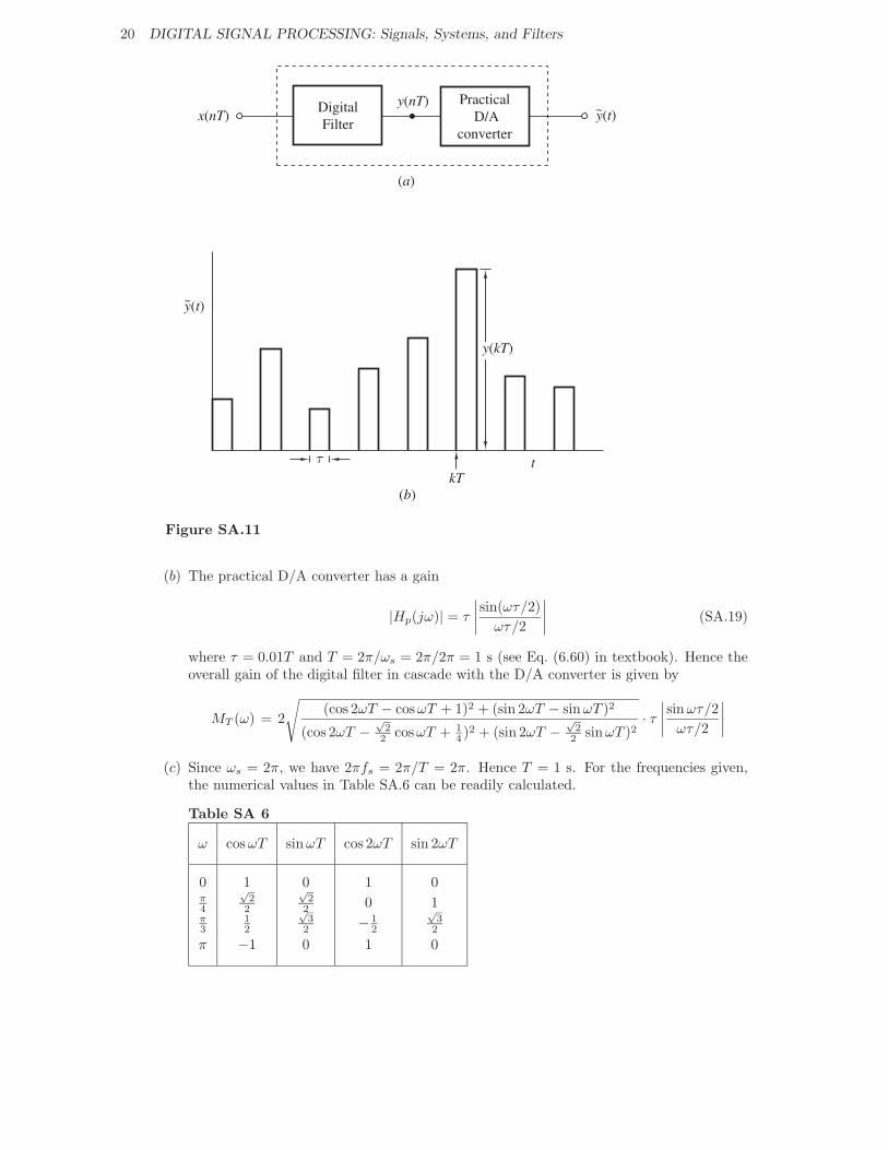
∣∣∣∣(c) Since ωs = 2π, we have 2πfs = 2π/T = 2π. Hence T = 1 s. For the frequencies given,
the numerical values in Table SA.6 can be readily calculated.
Table SA 6
ω cos ωT sin ωT cos 2ωT sin 2ωT
0 1 0 1 0π4
√2
2
√2
2 0 1π3
12
√3
2 −12
√3
2
π −1 0 1 0
SAMPLE SOLUTIONS 21
Thus
M(0) = 2
√(1 − 1 + 1)2 + (0 − 0)2
(1 −√
22 + 1
4 )2 + (0 − 0)2=
25−2
√2
4
= 3.6840
M(π
4
)= 2
√√√√ (0 −√
22 + 1)2 + (1 −
√2
2 )2
(0 −√
22 ×
√2
2 + 14 )2 + (1 −
√2
2 ×√
22 )2
= 2
√(2 −√
2)2 + (2 −√2)2
( 12 − 1)2 + 1
= 2
√2(2 −√
2)2
(−12 )2 + 1
= 1.4890
M(π
3
)= 2
√√√√ (−12 − 1
2 + 1)2 + (√
32 −
√3
2 )2
(−12 −
√2
2 × 12 + 1
4 )2 + (√
32 −
√2
2 ×√
32 )
= 2
√√√√ 0 + 0(1−2−√
24
)2
+ · · ·= 0
M(π) = 2
√(1 + 1 + 1)2 + (0 − 0)
(1 +√
22 + 1
4 )2 + (0 − 0)= 2
√32 × 16
(4 + 2√
2 + 1)2
=2 × 3 × 4
4 + 2√
2 + 1= 3.0657
(d) Since T = 1s, Eq. (SA.19) gives
|HP (jω)| = 0.01T
∣∣∣∣ sin(0.01Tω/2)0.01Tω/2
∣∣∣∣ = 0.01∣∣∣∣ sin(0.01ω/2)
0.01ω/2
∣∣∣∣= p0.01
Hence the overall gain of the digital filter in cascade with the D/A converter is obtainedfrom the above numerical values as follows:
MT (0) = 3.6840 × 0.01 = 3.6840 × 10⁻²
MT
(π
4
)= 1.4890 × 0.01 = 1.4890 × 10⁻²
MT
(π
3
)= 0 × 0.0100 = 0.0
MT (π) = 3.0557 × 0.01 = 3.0557 × 10⁻²
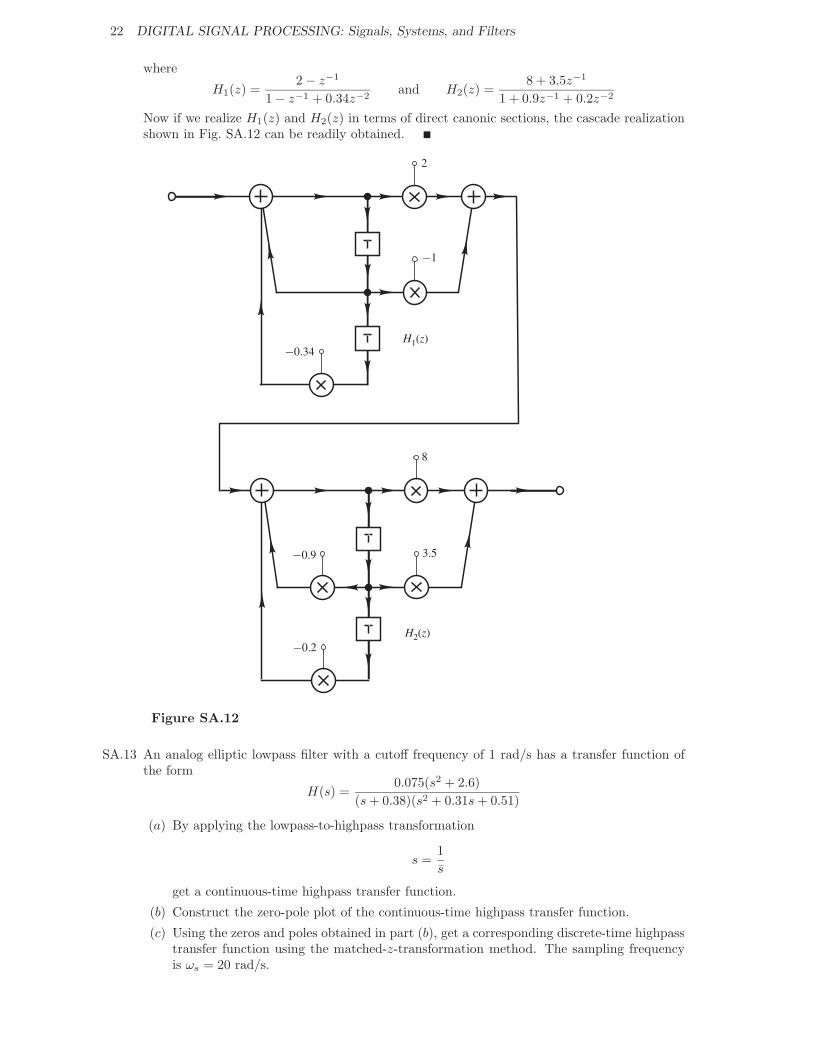
SA.12 Realize the transfer function
H(z) =(
z
z − 0.5 + j0.3+
z
z − 0.5 − j0.3
)·(
3z
z + 0.4+
5z
z + 0.5
)
using two second-order canonic filter sections in cascade.
Solution
The transfer function can be expressed as
H(z) =2z2 − 0.5z − 0.5z
z2 − z + 0.52 + 0.32· 3z2 + 1.5z + 5z2 + 2z
z2 + 0.9z + 0.2
=2z2 − z
z2 − z + 0.34· 8z2 + 3.5z
z2 + 0.9z + 0.2
=2 − z−1
1 − z−1 + 0.34z−2· 8 + 3.5z−1
1 + 0.9z−1 + 0.2z−2
= H1(z) · H2(z)
22 DIGITAL SIGNAL PROCESSING: Signals, Systems, and Filters
where
H1(z) =2 − z−1
1 − z−1 + 0.34z−2and H2(z) =
8 + 3.5z−1
1 + 0.9z−1 + 0.2z−2
Now if we realize H1(z) and H2(z) in terms of direct canonic sections, the cascade realizationshown in Fig. SA.12 can be readily obtained.
3.5
8
−0.2
−0.9
−1
2
−0.34 H1(z)
H2(z)
Figure SA.12
SA.13 An analog elliptic lowpass filter with a cutoff frequency of 1 rad/s has a transfer function ofthe form
H(s) =0.075(s2 + 2.6)
(s + 0.38)(s2 + 0.31s + 0.51)
(a) By applying the lowpass-to-highpass transformation
s =1s̄
get a continuous-time highpass transfer function.
(b) Construct the zero-pole plot of the continuous-time highpass transfer function.
(c) Using the zeros and poles obtained in part (b), get a corresponding discrete-time highpasstransfer function using the matched-z-transformation method. The sampling frequencyis ωs = 20 rad/s.
SAMPLE SOLUTIONS 23
(d) How does the matched-z-transformation method compare with the invariant-impulse-response method?
Solution
The transfer function has zeros atz = z1, z∗1
wherez1 = 0 + j1.6125
and poles atz = p0, p1, p∗1
where
p0 = −0.3800 + j0.0000p1 = −0.1550 + j0.6971
(a) The highpass transfer function is obtained as
HHP (s̄) = H(s)∣∣∣∣s̄→ 1
s
=0.075(s̄2 + 2.6)
(s + 0.38)(s2 + 0.31s + 0.51)
∣∣∣∣s=1/s̄
=0.075( 1
s̄2 + 2.6)( 1
s̄ + 0.38)( 1s̄2 + 0.31 1
s̄ + 0.51)
=0.075s̄(1 + 2.6s̄2)
(1 + 0.38s̄)(0.51s̄2 + 0.31s̄ + 1)
=0.075 × 2.60.38 × 0.51
× s̄(s̄2 + 12.6 )
(s̄ + 10.38 )(s̄2 + 0.31
0.51 s̄ + 10.51 )
= 1.0063 × s̄(s̄2 + 0.3846)(s̄ + 2.6316)(s̄2 + 0.6079s̄ + 1.9609)
Therefore, the highpass filter has zeros at
s̄ = s̄0, s̄1, s̄2
wheres̄0 = 0, s̄1, s̄2 = 0 ± j0.6202
and poles ats̄ = p̄0, p̄1, p̄2
wherep̄0 = −2.6316, p̄1, p̄2 = −0.3040 ± j1.3669
(b) The transfer function of the digital filter is given by
HD(z) = (z + 1)L
H0
M∏i=1
(z − es̄iT )
N∏i=1
(z − ep̄iT )
where L = 0 for a highpass filter. Hence
HD(z) =
3∏i=1
(z − z̃i)
3∏i=1
(z − p̃i)
24 DIGITAL SIGNAL PROCESSING: Signals, Systems, and Filters
where
z̃0 = e0T = 1, z̃1, z̃2 = e±j0.6202T
p̃0 = e−2.6316T , p̃1, p̃2 = e(−0.3040±j1.3669)T
withT =
2π
ωs=
2π
20=
π
10
(c) The method works with all types of filters, i.e., LP, HP, BP, and BS, and is easy to apply.However, it tends to increase the passband ripple.
SA.14 A lowpass analog filter has a transfer function
HA(s) =1
s2 +√
2s + 1
(a) Assuming a sampling frequency of 10π, design a digital filter using the bilinear transfor-mation method.
(b) Find the 1-dB and 30-dB frequencies of the analog filter.
(c) Find the 1-dB and 30-dB frequencies of the digital filter.
(d) What should be the 3-dB frequency of the analog filter to get a 3-dB frequency in thedigital filter at 1 rad/s?
Solution
(a) The sampling period is give by
T =1fs
=2π
ωs=
2π
10π=
15
The discrete-time transfer function is given by
HD(z) = HA(s)∣∣s= 2
Tz−1z+1
=1
s2 +√
2s + 1
∣∣∣∣∣s= 10(z−1)
z+1
=1[
10(z−1)z+1
]2+√
2[
10(z−1)z+1
]+ 1
=z2 + 2z + 1
100(z2 − 2z + 1) + 10√
2(z2 − 1) + (z2 + 2z + 1)
=z2 + 2z + 1
b2z2 + b1z + b0
where
b0 = 100 − 10√
2 + 1 = 86.86b1 = −200 + 2 = −198.00b2 = 100 + 10
√2 + 1 = 115.14
Alternatively, by factorizing constant b2 in the denominator, the transfer function can beexpressed as
HD(z) = H0z2 + 2z + 1
z2 + b′1z + b′0where
H0 = 8.685 × 10⁻³, b′0 = 0.7544, b′1 = −1.720
SAMPLE SOLUTIONS 25
(b) The frequency response of the analog filter
HA(jω) =1
−ω2 + j√
2ω + 1
Hence the loss is given by
A(ω) = 20 log√
(1 − ω2)2 + 2ω2
= 10 log(1 − 2ω2 + ω4 + 2ω2)
Thus1 + ω4 = 100.1×A(ω)
By letting A(ω) = 1 dB, the 1-dB frequency is obtained as
ω1 = (100.1 − 1)1/4 = 0.7133 rad/s
By letting A(ω) = 30 dB, the 30-dB frequency is obtained as
ω2 = (100.1×30 − 1)1/4 = 5.622 rad/s
(c) A frequency ωi in the analog filter transforms into a frequency Ωi given by
Ωi =2T
tan−1 ωiT
2(SA.20)
Hence the 1- and 30-dB frequencies in the digital filter are obtained as
Ω1 = 10 × tan−1 0.713310
= 0.7121 rad/s
andΩ2 = 10 × tan−1 5.622
10= 5.122 rad/s
respectively.
(d) Now if the 3-dB frequency in the digital filter is required to be 1 rad/s, then accordingto Eq. (SA.20) the 3-dB frequency in the analog filter should be
ω3 =2T
tanΩ3T
2= 10 × tan
110
= 1.003 rad/s