rspa.royalsocietypublishing.org

Research

Article submitted to journal

Subject Areas:

power and energy systems,

acoustics, thermodynamics

Keywords:

combustion instabilities, flame

describing function, H∞

loop-shaping, ν-gap metric, level set

approach, low order controller

Author for correspondence:

Jingxuan Li

e-mail: ljx.buaa@gmail.com

Feedback control ofcombustion instabilities fromwithin limit cycle oscillationsusing H∞ loop-shaping andthe ν-gap metricJingxuan Li1 and Aimee S. Morgans1

1Department of Mechanical Engineering, Imperial

College London, London, UK

Combustion instabilities arise due to a two-waycoupling between acoustic waves and unsteadyheat release. Oscillation amplitudes successivelygrow, until nonlinear effects cause saturation intolimit cycle oscillations. Feedback control, in whichan actuator modifies some combustor input inresponse to a sensor measurement, can suppresscombustion instabilities. Linear feedback controllersare typically designed using linear combustor models.However, when activated from within limit cycle,the linear model is invalid and such controllers arenot guaranteed to stabilise. This work develops afeedback control strategy guaranteed to stabilise fromwithin limit cycle oscillations. A low order model ofa simple combustor, exhibiting the essential featuresof more complex systems, is presented. Linear planeacoustic wave modelling is combined with a weaklynonlinear describing function for the flame. The latteris determined numerically using a level set approach.Its implication is that the open loop transfer function(OLTF) needed for controller design varies withoscillation level. The difference between the mean andthe rest of OLTFs is characterised using the ν-gapmetric, providing the minimum required “robustnessmargin” for an H∞ loop-shaping controller. Suchcontrollers are designed and achieve stability bothfor linear fluctuations and from within limit cycleoscillations.

1. IntroductionIt is desirable to operate modern industrial gas turbinesand aero-engines under lean premixed combustion

c© The Authors. Published by the Royal Society under the terms of the

Creative Commons Attribution License http://creativecommons.org/licenses/

by/4.0/, which permits unrestricted use, provided the original author and

source are credited.

2

rspa.royalsocietypublishing.orgP

rocR

Soc

A0000000

..........................................................

conditions in order to reduce NOx emissions. However, lean premixed systems are highlysusceptible to combustion instabilities arising from the coupling between the heat releaserate perturbations and the acoustic disturbances within the combustion chamber [1]. Theseinstabilities are nearly always undesirable as they lead to large oscillation amplitudes anddamaging structural vibrations of the combustion chamber [2].

The stability of a combustion chamber is determined by the balance between the energy gainedfrom the flame/acoustic interactions and various dissipation processes [1,3,4]. Active feedbackcontrol can be used to interrupt the coupling between the acoustic waves and unsteady heatrelease and prevent or suppress instability. The design of most types of controller requires priorknowledge of how the combustor responds to actuation — the “open loop transfer function”(OLTF) between monitored thermodynamic properties within the combustion chamber (typicallyone or more pressure measurements) and the actuator signal(s) [4].

Although linear models may be accurate at low perturbation levels, the dynamics of realunstable combustors become dominated by nonlinear mechanisms once amplitudes growsufficiently. In many combustors, including gas turbine and aero-engine combustors, it is notablethat even during large amplitude oscillations, the behaviour of the acoustic waves remains linear,with nonlinearity arising almost entirely from the way in which the flame’s unsteady heat releaseresponds to oncoming flow disturbances [5–7]. (Acoustic waves in rocket engines are, however,typically nonlinear [8].) This flame nonlinearity is “weak” such that a “describing function”provides a good model of the nonlinear flame response. This assumes that the flow forcingamplitude level is a quasi-steady parameter, and that the dominant frequency of the unsteadyheat release rate response matches the incoming flow forcing frequency, but with a gain andphase shift that depend on the forcing level as well as the frequency. This gives rise to a “family” offrequency responses which depend on forcing level. It has been shown that this weak nonlinearitycan cause saturation into limit cycle either via saturation of the heat release rate amplitude or viaa change in phase between the heat release rate and acoustic pressure as the modulation levelincreases [6,9]. This may cause the dominant unstable frequency to change, which in turn altersthe OLTF and complicates controller design. Although some recent work has identified nonlinearstates other than limit cycle oscillations as resulting from combustion instability [10–12], the focusof the current work will be limit cycle oscillations, which are by far the most common reportednonlinear state.

The design of linear feedback controllers is typically based on the OLTF corresponding tosmall, linear disturbances. Such feedback controllers are then activated from within nonlinearlimit cycle oscillations, during which the linear OLTF will not be valid. It is typically observedthat such controllers successfully stabilise oscillations despite this paradox [13–15]. However,their effectiveness is not guaranteed, and if they fail there has until now been no frameworkfor systematically improving their design.

In this work, the concept of a flame describing function (FDF) is combined with the ν-gapmetric [16] in order to design controllers which are guaranteed to achieve stabilisation across alloscillation levels, from small linear fluctuations to large limit cycle oscillations. In modern robustcontrol systems theory, the concept of a ν-gap between open loop plants represents the mostuseful measure of distance between systems when one is concerned specifically with applyingfeedback to those systems. The ν-gap metric fits very naturally into H∞ loop-shaping controllerdesign, providing a bound on the minimum required “robustness stability margin” for an H∞loop-shaping controller [16,17]. Modern linear robust control, of which H∞ loop-shaping isone methodology, has been successfully used in diverse fields, such as control of combustioninstabilities [18–20], control of developing flow [21], voltage converter design [22] and vehicleoscillation damper optimisation [23], to achieve control even in nonlinear systems with limitcycles. H∞ loop-shaping combines classical loop-shaping, which can obtain tradeoffs betweengood performance and robust stability, with modern H∞ optimisation in order to guaranteeclosed-loop stability and a level of robust stability at all frequencies [16,17]. It can be appliedto plants with high dimensions and is computationally inexpensive [19], at least for plants of low

3

rspa.royalsocietypublishing.orgP

rocR

Soc

A0000000

..........................................................

flame

microphone

loudspeaker

controller

external signal

pL

A+1 A−

1

A+2 A−

2

u1

u2

x = x0

x = x1 = xf

x = x2

x = xr

+−

D

d

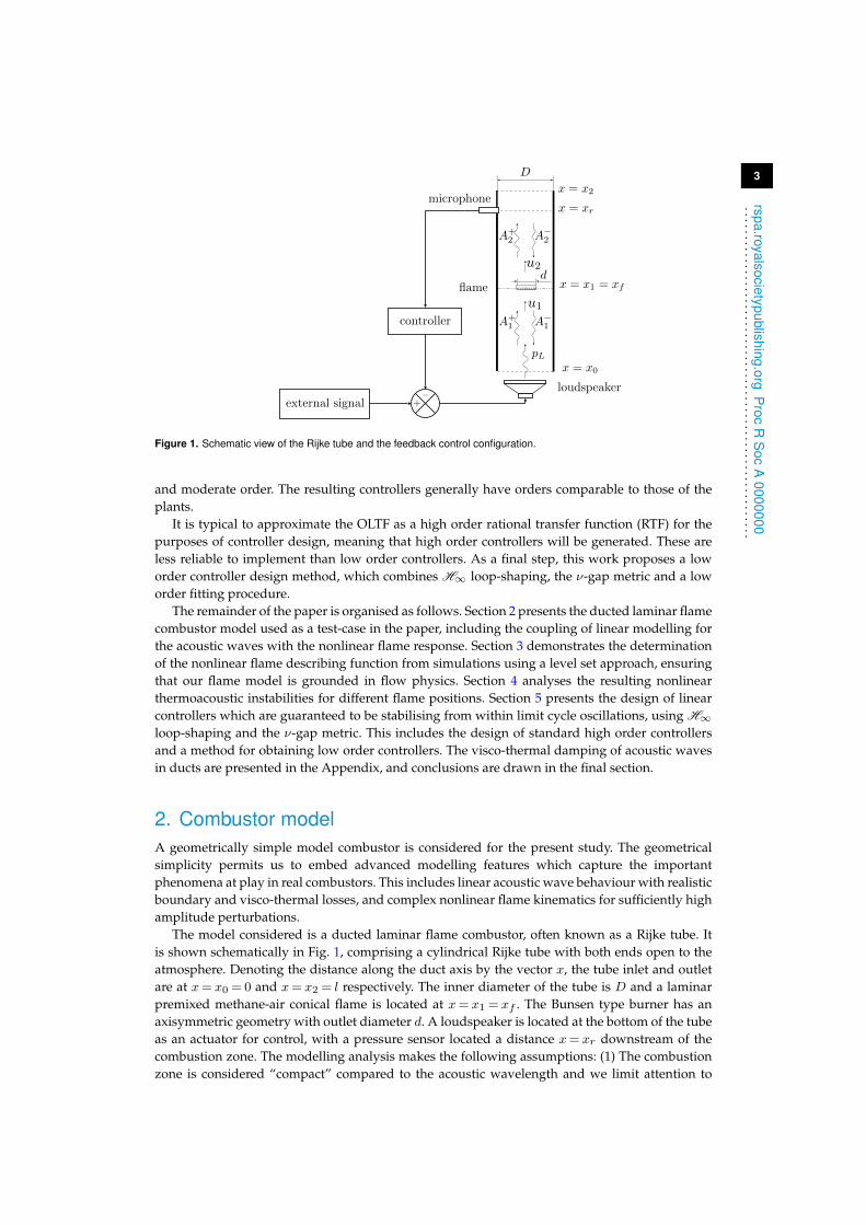
Figure 1. Schematic view of the Rijke tube and the feedback control configuration.

and moderate order. The resulting controllers generally have orders comparable to those of theplants.

It is typical to approximate the OLTF as a high order rational transfer function (RTF) for thepurposes of controller design, meaning that high order controllers will be generated. These areless reliable to implement than low order controllers. As a final step, this work proposes a loworder controller design method, which combines H∞ loop-shaping, the ν-gap metric and a loworder fitting procedure.

The remainder of the paper is organised as follows. Section 2 presents the ducted laminar flamecombustor model used as a test-case in the paper, including the coupling of linear modelling forthe acoustic waves with the nonlinear flame response. Section 3 demonstrates the determinationof the nonlinear flame describing function from simulations using a level set approach, ensuringthat our flame model is grounded in flow physics. Section 4 analyses the resulting nonlinearthermoacoustic instabilities for different flame positions. Section 5 presents the design of linearcontrollers which are guaranteed to be stabilising from within limit cycle oscillations, using H∞loop-shaping and the ν-gap metric. This includes the design of standard high order controllersand a method for obtaining low order controllers. The visco-thermal damping of acoustic wavesin ducts are presented in the Appendix, and conclusions are drawn in the final section.

2. Combustor modelA geometrically simple model combustor is considered for the present study. The geometricalsimplicity permits us to embed advanced modelling features which capture the importantphenomena at play in real combustors. This includes linear acoustic wave behaviour with realisticboundary and visco-thermal losses, and complex nonlinear flame kinematics for sufficiently highamplitude perturbations.

The model considered is a ducted laminar flame combustor, often known as a Rijke tube. Itis shown schematically in Fig. 1, comprising a cylindrical Rijke tube with both ends open to theatmosphere. Denoting the distance along the duct axis by the vector x, the tube inlet and outletare at x= x0 = 0 and x= x2 = l respectively. The inner diameter of the tube is D and a laminarpremixed methane-air conical flame is located at x= x1 = xf . The Bunsen type burner has anaxisymmetric geometry with outlet diameter d. A loudspeaker is located at the bottom of the tubeas an actuator for control, with a pressure sensor located a distance x= xr downstream of thecombustion zone. The modelling analysis makes the following assumptions: (1) The combustionzone is considered “compact” compared to the acoustic wavelength and we limit attention to

4

rspa.royalsocietypublishing.orgP

rocR

Soc

A0000000

..........................................................

low frequencies where we only need to account for longitudinal waves [24]. (2) The fluids beforeand after the flame are assumed to be perfect gases [24]. (3) There is no noise produced by theentropy waves formed during the unstable combustion process — these waves are assumed toleave the tube without interaction with the flow at the end of tube [25]. (4) The flame remainsstabilised at the burner outlet. Flame intrinsic instabilities [26] and irregular response to strongdisturbances [27] are not accounted for.

The flow can be taken to be composed of a steady uniform mean flow (denoted ¯ )and small perturbations (denoted ′). Harmonic time variations are considered for which allfluctuating variables have the form a′ = aeiωt, where ω is complex angular frequency. The regionsupstream and downstream of the flame are indicated by the subscripts 1 and 2 respectively.Then, the pressure, p, and longitudinal velocity, u, in the two regions can be expressed interms of the amplitudes A+

n and A−n of the upward and downward propagating acousticwaves respectively, their wavenumbers, k± = k± +∆k±, where k± = ω/(c± u) and ∆k± arewavenumber corrections for the visco-thermal damping effects (see Appendix), and the speed ofsound, c, and density, ρ [28]. The pressure, p, and longitudinal velocity, u, in the two regions areexpressed as:

pn(x, t) = pn + pn(x)eiωt = pn +(A+n e

ik+n (x−xn−1) +A−n e−ik−n (x−xn−1)

)eiωt (n= 1, 2)

un(x, t) = un + un(x)eiωt = un +1

ρncn

(A+n e

ik+n (x−xn−1) −A−n e−ik−n (x−xn−1)

)eiωt.

(2.1)

The acoustic wave strengths, A+n and A−n , are related by pressure reflection coefficients1 at the

tube boundaries – the inlet and outlet pressure reflection coefficients are characterized by R1 andR2 respectively.

For an open duct, radiation of sound from the duct ends can be accounted for using frequencydependent reflection coefficients which act as low-pass filters [29]. The tube also appearsacoustically longer than its physical length and this end correction can be accounted for. Thereflection coefficient for an unflanged pipe end can be approximately expressed in the Laplacedomain as [29,30]:

R=−(1 + 2τ2

d s2)e−0.61τds for 2πfτd� 1. (2.2)

where τd =D/c. It was confirmed in [31] that the gain of this reflection coefficient decreases withboth duct diameter and frequency. The reflection coefficients at the inlet and outlet of the Rijketube are denoted by R1 and R2 respectively.

In order to relate the acoustic wave strengths across the flame, the linearised mass, momentumand energy conservation equations across the flame zone (x= xf ) are combined with the perfectgas equation. Denoting the jump across the flame as [·]21, the amplitude of the flame’s heat release

rate perturbation as Q and the cross-sectional area of the duct as S, this yields two equationswhich are independent of the downstream density, ρ2, which contains an entropy component [32]:

S2

S1

[p(xf )

]21

+ ρ1u1

[u(xf )

]21

+ [u]21

(ρ1u1(xf ) +

p1(xf )

c21u1

)= 0 (2.3)

γ

γ − 1

[S(pu(xf ) + p(xf )u

)]21

+ ρ1u1S1

[uu(xf )

]21

= Q. (2.4)

Note that upstream of the flame, S1 = π(D2 − d2)/4. γ is the ratio of specific heats of thegases, considered constant throughout the duct due to the small temperature jump across theflame. Substituting the linearised pressure and velocity expressions from Eq. (2.1) together withthe boundary conditions into the above two conservation equations, the governing equationslinking the acoustic wave strengths before and after the flame are obtained in terms of s, theLaplace transform variable [33] (where sn = s+ Λn

√s, n= 1, 2, the second term accounting for

1The pressure reflection coefficient is defined as the ratio of reflected to incident acoustic waves at the boundary [24].

5

rspa.royalsocietypublishing.orgP

rocR

Soc

A0000000

..........................................................

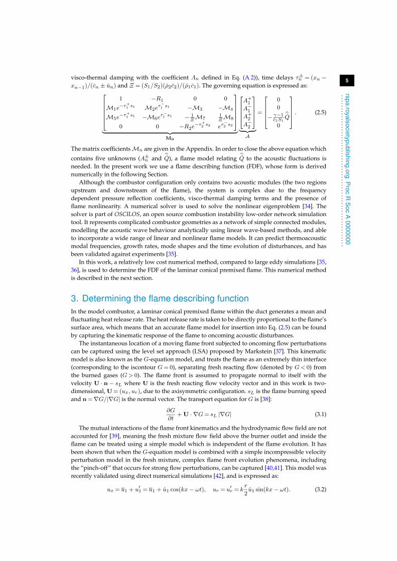
visco-thermal damping with the coefficient Λn defined in Eq. (A 2)), time delays τ±n = (xn −xn−1)/(cn ± un) and Ξ = (S1/S2)(ρ2c2)/(ρ1c1). The governing equation is expressed as:

1 −R1 0 0

M1e−τ+

1 s1 M2eτ−1 s1 −M3 −M4

M5e−τ+

1 s1 −M6eτ−1 s1 − 1

ΞM71ΞM8

0 0 −R2e−τ+

2 s2 eτ−2 s2

︸ ︷︷ ︸

M0

A+

1

A−1A+

2

A−2

︸ ︷︷ ︸A

=

0

0

− γ−1c1S1

Q0

. (2.5)

The matrix coefficientsMn are given in the Appendix. In order to close the above equation which

contains five unknowns (A±n and Q), a flame model relating Q to the acoustic fluctuations isneeded. In the present work we use a flame describing function (FDF), whose form is derivednumerically in the following Section.

Although the combustor configuration only contains two acoustic modules (the two regionsupstream and downstream of the flame), the system is complex due to the frequencydependent pressure reflection coefficients, visco-thermal damping terms and the presence offlame nonlinearity. A numerical solver is used to solve the nonlinear eigenproblem [34]. Thesolver is part of OSCILOS, an open source combustion instability low-order network simulationtool. It represents complicated combustor geometries as a network of simple connected modules,modelling the acoustic wave behaviour analytically using linear wave-based methods, and ableto incorporate a wide range of linear and nonlinear flame models. It can predict thermoacousticmodal frequencies, growth rates, mode shapes and the time evolution of disturbances, and hasbeen validated against experiments [35].

In this work, a relatively low cost numerical method, compared to large eddy simulations [35,36], is used to determine the FDF of the laminar conical premixed flame. This numerical methodis described in the next section.

3. Determining the flame describing functionIn the model combustor, a laminar conical premixed flame within the duct generates a mean andfluctuating heat release rate. The heat release rate is taken to be directly proportional to the flame’ssurface area, which means that an accurate flame model for insertion into Eq. (2.5) can be foundby capturing the kinematic response of the flame to oncoming acoustic disturbances.

The instantaneous location of a moving flame front subjected to oncoming flow perturbationscan be captured using the level set approach (LSA) proposed by Markstein [37]. This kinematicmodel is also known as the G-equation model, and treats the flame as an extremely thin interface(corresponding to the iscontour G= 0), separating fresh reacting flow (denoted by G< 0) fromthe burned gases (G> 0). The flame front is assumed to propagate normal to itself with thevelocity U · n− sL where U is the fresh reacting flow velocity vector and in this work is two-dimensional, U = (ux, ur), due to the axisymmetric configuration. sL is the flame burning speedand n =∇G/|∇G| is the normal vector. The transport equation for G is [38]:

∂G

∂t+ U · ∇G= sL |∇G| (3.1)

The mutual interactions of the flame front kinematics and the hydrodynamic flow field are notaccounted for [39], meaning the fresh mixture flow field above the burner outlet and inside theflame can be treated using a simple model which is independent of the flame evolution. It hasbeen shown that when the G-equation model is combined with a simple incompressible velocityperturbation model in the fresh mixture, complex flame front evolution phenomena, includingthe “pinch-off” that occurs for strong flow perturbations, can be captured [40,41]. This model wasrecently validated using direct numerical simulations [42], and is expressed as:

ux = u1 + u′1 = u1 + u1 cos(kx− ωt), ur = u′r = kr

2u1 sin(kx− ωt). (3.2)

6

rspa.royalsocietypublishing.orgP

rocR

Soc

A0000000

..........................................................

−20 −10 0 10 20

0

10

20

30

40

r [mm]x[m

m]

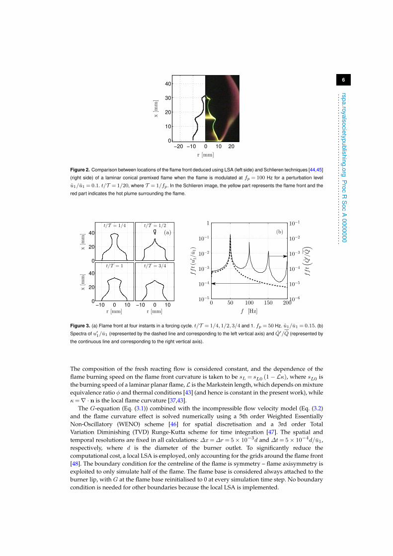
Figure 2. Comparison between locations of the flame front deduced using LSA (left side) and Schlieren techniques [44,45]

(right side) of a laminar conical premixed flame when the flame is modulated at fp = 100 Hz for a perturbation level

u1/u1 = 0.1. t/T = 1/20, where T = 1/fp. In the Schlieren image, the yellow part represents the flame front and the

red part indicates the hot plume surrounding the flame.

0

20

40

x[m

m]

t/T = 1/4 t/T = 1/2

(a)

−10 0 10

r [mm]

t/T = 3/4

−10 0 100

20

40

r [mm]

x[m

m]

t/T = 1

f [Hz]

fft(u

′ 1/u1)

10−5

10−4

10−3

10−2

10−1

1

0 50 100 150 200fft(

Q′/Q

)10−6

10−5

10−4

10−3

10−2

10−1

(b)

Figure 3. (a) Flame front at four instants in a forcing cycle. t/T = 1/4, 1/2, 3/4 and 1. fp = 50 Hz. u1/u1 = 0.15. (b)

Spectra of u′1/u1 (represented by the dashed line and corresponding to the left vertical axis) and Q′/Q (represented by

the continuous line and corresponding to the right vertical axis).

The composition of the fresh reacting flow is considered constant, and the dependence of theflame burning speed on the flame front curvature is taken to be sL = sL0 (1− Lκ), where sL0 isthe burning speed of a laminar planar flame,L is the Markstein length, which depends on mixtureequivalence ratio φ and thermal conditions [43] (and hence is constant in the present work), whileκ=∇ · n is the local flame curvature [37,43].

The G-equation (Eq. (3.1)) combined with the incompressible flow velocity model (Eq. (3.2)and the flame curvature effect is solved numerically using a 5th order Weighted EssentiallyNon-Oscillatory (WENO) scheme [46] for spatial discretisation and a 3rd order TotalVariation Diminishing (TVD) Runge-Kutta scheme for time integration [47]. The spatial andtemporal resolutions are fixed in all calculations: ∆x=∆r= 5× 10−3d and ∆t= 5× 10−4d/u1,respectively, where d is the diameter of the burner outlet. To significantly reduce thecomputational cost, a local LSA is employed, only accounting for the grids around the flame front[48]. The boundary condition for the centreline of the flame is symmetry – flame axisymmetry isexploited to only simulate half of the flame. The flame base is considered always attached to theburner lip, with G at the flame base reinitialised to 0 at every simulation time step. No boundarycondition is needed for other boundaries because the local LSA is implemented.

7

rspa.royalsocietypublishing.orgP

rocR

Soc

A0000000

..........................................................

0 40 80 120 160−8

−6

−4

−2

0

f [Hz]

6F/π

(a)

0.2

0.4

0.6

0.8

1|F

|

u1/u1 = 0.036u1/u1 = 0.071u1/u1 = 0.143u1/u1 = 0.214

0 40 80 120 160−8

−6

−4

−2

0

f [Hz]

6F/π

(b)

0.2

0.4

0.6

0.8

1

|F|

u1/u1 = 0.036u1/u1 = 0.071u1/u1 = 0.143u1/u1 = 0.214

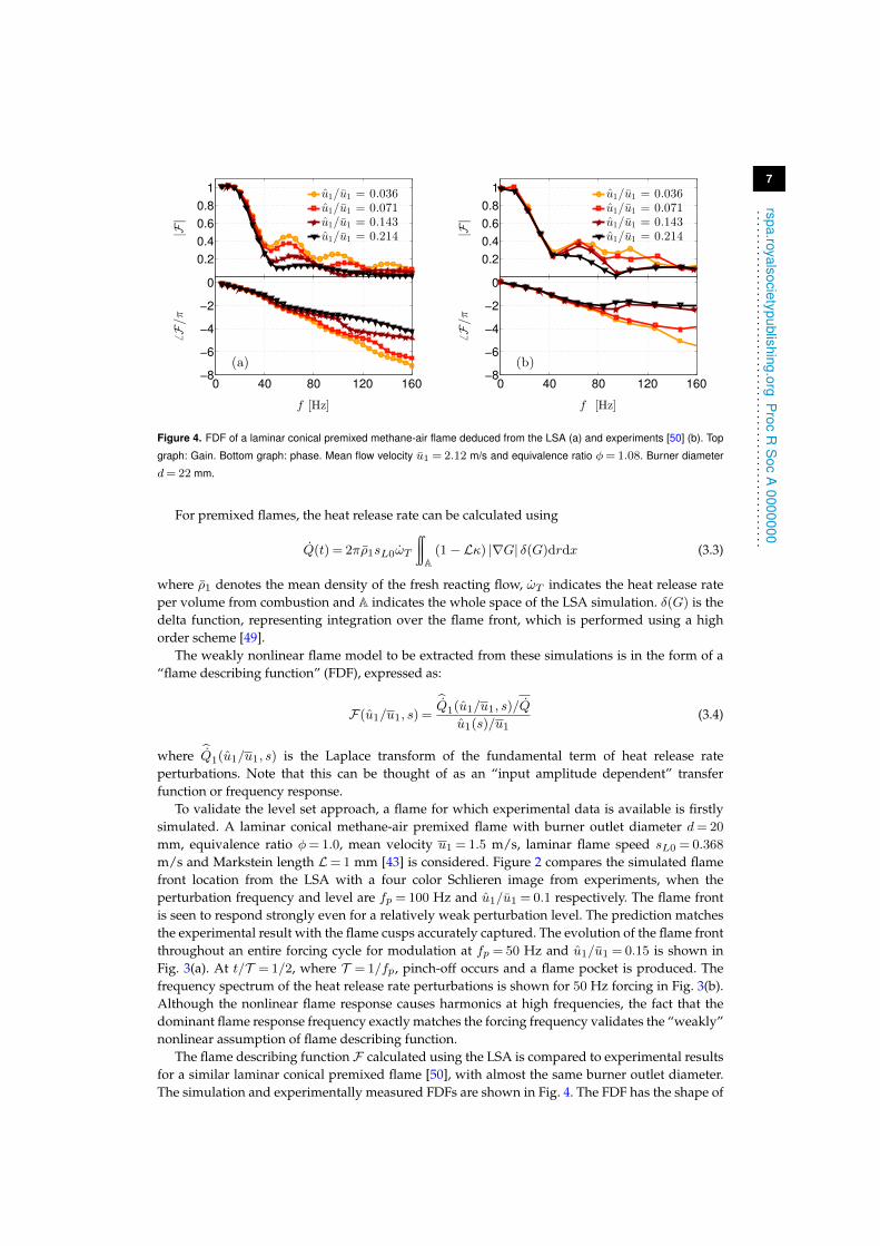
Figure 4. FDF of a laminar conical premixed methane-air flame deduced from the LSA (a) and experiments [50] (b). Top

graph: Gain. Bottom graph: phase. Mean flow velocity u1 = 2.12 m/s and equivalence ratio φ= 1.08. Burner diameter

d= 22 mm.

For premixed flames, the heat release rate can be calculated using

Q(t) = 2πρ1sL0ωT

∫∫A

(1− Lκ) |∇G| δ(G)drdx (3.3)

where ρ1 denotes the mean density of the fresh reacting flow, ωT indicates the heat release rateper volume from combustion and A indicates the whole space of the LSA simulation. δ(G) is thedelta function, representing integration over the flame front, which is performed using a highorder scheme [49].

The weakly nonlinear flame model to be extracted from these simulations is in the form of a“flame describing function” (FDF), expressed as:

F(u1/u1, s) =Q1(u1/u1, s)/Q

u1(s)/u1(3.4)

where Q1(u1/u1, s) is the Laplace transform of the fundamental term of heat release rateperturbations. Note that this can be thought of as an “input amplitude dependent” transferfunction or frequency response.

To validate the level set approach, a flame for which experimental data is available is firstlysimulated. A laminar conical methane-air premixed flame with burner outlet diameter d= 20

mm, equivalence ratio φ= 1.0, mean velocity u1 = 1.5 m/s, laminar flame speed sL0 = 0.368

m/s and Markstein length L= 1 mm [43] is considered. Figure 2 compares the simulated flamefront location from the LSA with a four color Schlieren image from experiments, when theperturbation frequency and level are fp = 100 Hz and u1/u1 = 0.1 respectively. The flame frontis seen to respond strongly even for a relatively weak perturbation level. The prediction matchesthe experimental result with the flame cusps accurately captured. The evolution of the flame frontthroughout an entire forcing cycle for modulation at fp = 50 Hz and u1/u1 = 0.15 is shown inFig. 3(a). At t/T = 1/2, where T = 1/fp, pinch-off occurs and a flame pocket is produced. Thefrequency spectrum of the heat release rate perturbations is shown for 50 Hz forcing in Fig. 3(b).Although the nonlinear flame response causes harmonics at high frequencies, the fact that thedominant flame response frequency exactly matches the forcing frequency validates the “weakly”nonlinear assumption of flame describing function.

The flame describing function F calculated using the LSA is compared to experimental resultsfor a similar laminar conical premixed flame [50], with almost the same burner outlet diameter.The simulation and experimentally measured FDFs are shown in Fig. 4. The FDF has the shape of

8

rspa.royalsocietypublishing.orgP

rocR

Soc

A0000000

..........................................................

0100

200300

400500 0

0.10.2

0.30.4

0

0.2

0.4

0.6

0.8

1

u1/u1f [Hz]

|F

|

(a)

0100

200300

400500 0

0.10.2

0.30.4

−6

−4

−2

0

u1/u1f [Hz]

6(F

)/π

(b)

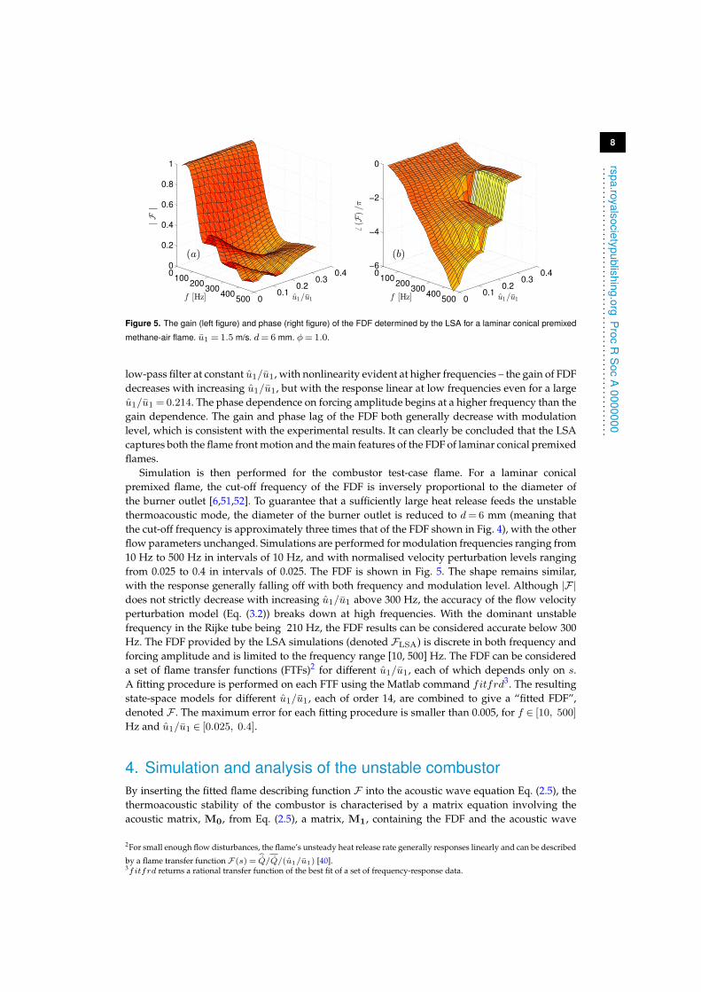
Figure 5. The gain (left figure) and phase (right figure) of the FDF determined by the LSA for a laminar conical premixed

methane-air flame. u1 = 1.5 m/s. d= 6 mm. φ= 1.0.

low-pass filter at constant u1/u1, with nonlinearity evident at higher frequencies – the gain of FDFdecreases with increasing u1/u1, but with the response linear at low frequencies even for a largeu1/u1 = 0.214. The phase dependence on forcing amplitude begins at a higher frequency than thegain dependence. The gain and phase lag of the FDF both generally decrease with modulationlevel, which is consistent with the experimental results. It can clearly be concluded that the LSAcaptures both the flame front motion and the main features of the FDF of laminar conical premixedflames.

Simulation is then performed for the combustor test-case flame. For a laminar conicalpremixed flame, the cut-off frequency of the FDF is inversely proportional to the diameter ofthe burner outlet [6,51,52]. To guarantee that a sufficiently large heat release feeds the unstablethermoacoustic mode, the diameter of the burner outlet is reduced to d= 6 mm (meaning thatthe cut-off frequency is approximately three times that of the FDF shown in Fig. 4), with the otherflow parameters unchanged. Simulations are performed for modulation frequencies ranging from10 Hz to 500 Hz in intervals of 10 Hz, and with normalised velocity perturbation levels rangingfrom 0.025 to 0.4 in intervals of 0.025. The FDF is shown in Fig. 5. The shape remains similar,with the response generally falling off with both frequency and modulation level. Although |F|does not strictly decrease with increasing u1/u1 above 300 Hz, the accuracy of the flow velocityperturbation model (Eq. (3.2)) breaks down at high frequencies. With the dominant unstablefrequency in the Rijke tube being 210 Hz, the FDF results can be considered accurate below 300Hz. The FDF provided by the LSA simulations (denoted FLSA) is discrete in both frequency andforcing amplitude and is limited to the frequency range [10, 500] Hz. The FDF can be considereda set of flame transfer functions (FTFs)2 for different u1/u1, each of which depends only on s.A fitting procedure is performed on each FTF using the Matlab command fitfrd3. The resultingstate-space models for different u1/u1, each of order 14, are combined to give a “fitted FDF”,denoted F . The maximum error for each fitting procedure is smaller than 0.005, for f ∈ [10, 500]

Hz and u1/u1 ∈ [0.025, 0.4].

4. Simulation and analysis of the unstable combustorBy inserting the fitted flame describing function F into the acoustic wave equation Eq. (2.5), thethermoacoustic stability of the combustor is characterised by a matrix equation involving theacoustic matrix, M0, from Eq. (2.5), a matrix, M1, containing the FDF and the acoustic wave

2For small enough flow disturbances, the flame’s unsteady heat release rate generally responses linearly and can be described

by a flame transfer function F(s) = Q/Q/(u1/u1) [40].3fitfrd returns a rational transfer function of the best fit of a set of frequency-response data.

9

rspa.royalsocietypublishing.orgP

rocR

Soc

A0000000

..........................................................

xf [m]

u1/u1

σ [s−1]

0.050.1 0.2 0.3 0.4 0.5

0.05

0.1

0.15

0.2

0.25

10

20

30

40

−300 −200 −100 0 100

100

200

300

400

500

Growth rate [s−1]

Eigenfrequency

[Hz]

u1/u1

zoomed

0.04

0.08

0.12

0.16

0.2

−20 0 20 40 60204

206

208

210

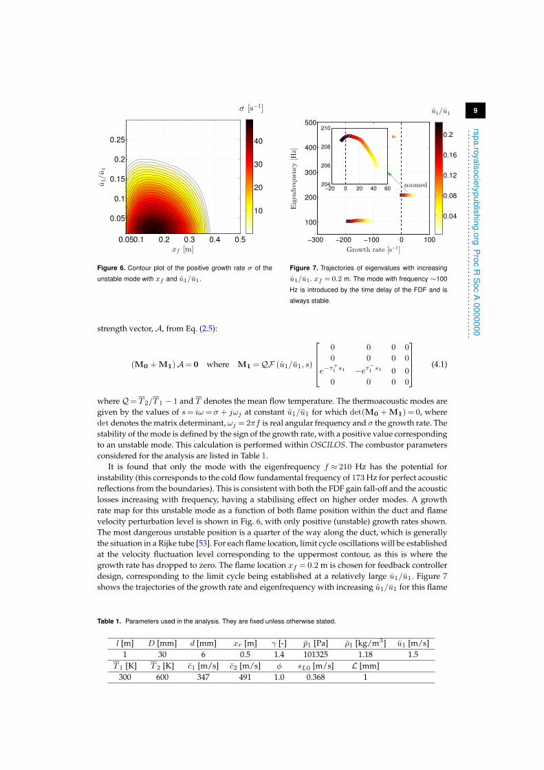
Figure 6. Contour plot of the positive growth rate σ of the

unstable mode with xf and u1/u1.

Figure 7. Trajectories of eigenvalues with increasing

u1/u1. xf = 0.2 m. The mode with frequency ∼100

Hz is introduced by the time delay of the FDF and is

always stable.

strength vector, A, from Eq. (2.5):

(M0 + M1)A= 0 where M1 =QF (u1/u1, s)

0 0 0 0

0 0 0 0

e−τ+1 s1 −eτ

−1 s1 0 0

0 0 0 0

(4.1)

whereQ= T 2/T 1 − 1 and T denotes the mean flow temperature. The thermoacoustic modes aregiven by the values of s= iω= σ + jωj at constant u1/u1 for which det(M0 + M1) = 0, wheredet denotes the matrix determinant, ωj = 2πf is real angular frequency and σ the growth rate. Thestability of the mode is defined by the sign of the growth rate, with a positive value correspondingto an unstable mode. This calculation is performed within OSCILOS. The combustor parametersconsidered for the analysis are listed in Table 1.

It is found that only the mode with the eigenfrequency f ≈ 210 Hz has the potential forinstability (this corresponds to the cold flow fundamental frequency of 173 Hz for perfect acousticreflections from the boundaries). This is consistent with both the FDF gain fall-off and the acousticlosses increasing with frequency, having a stabilising effect on higher order modes. A growthrate map for this unstable mode as a function of both flame position within the duct and flamevelocity perturbation level is shown in Fig. 6, with only positive (unstable) growth rates shown.The most dangerous unstable position is a quarter of the way along the duct, which is generallythe situation in a Rijke tube [53]. For each flame location, limit cycle oscillations will be establishedat the velocity fluctuation level corresponding to the uppermost contour, as this is where thegrowth rate has dropped to zero. The flame location xf = 0.2 m is chosen for feedback controllerdesign, corresponding to the limit cycle being established at a relatively large u1/u1. Figure 7shows the trajectories of the growth rate and eigenfrequency with increasing u1/u1 for this flame

Table 1. Parameters used in the analysis. They are fixed unless otherwise stated.

l [m] D [mm] d [mm] xr [m] γ [-] p1 [Pa] ρ1 [kg/m3] u1 [m/s]1 30 6 0.5 1.4 101325 1.18 1.5

T 1 [K] T 2 [K] c1 [m/s] c2 [m/s] φ sL0 [m/s] L [mm]300 600 347 491 1.0 0.368 1

10

rspa.royalsocietypublishing.orgP

rocR

Soc

A0000000

..........................................................

pL+

−

prP

W1 K∞

K

W2

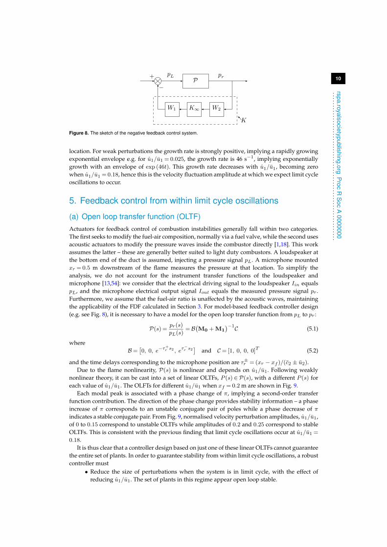
Figure 8. The sketch of the negative feedback control system.

location. For weak perturbations the growth rate is strongly positive, implying a rapidly growingexponential envelope e.g. for u1/u1 = 0.025, the growth rate is 46 s−1, implying exponentiallygrowth with an envelope of exp (46t). This growth rate decreases with u1/u1, becoming zerowhen u1/u1 = 0.18, hence this is the velocity fluctuation amplitude at which we expect limit cycleoscillations to occur.

5. Feedback control from within limit cycle oscillations

(a) Open loop transfer function (OLTF)Actuators for feedback control of combustion instabilities generally fall within two categories.The first seeks to modify the fuel-air composition, normally via a fuel valve, while the second usesacoustic actuators to modify the pressure waves inside the combustor directly [1,18]. This workassumes the latter – these are generally better suited to light duty combustors. A loudspeaker atthe bottom end of the duct is assumed, injecting a pressure signal pL. A microphone mountedxr = 0.5 m downstream of the flame measures the pressure at that location. To simplify theanalysis, we do not account for the instrument transfer functions of the loudspeaker andmicrophone [13,54]: we consider that the electrical driving signal to the loudspeaker Iin equalspL, and the microphone electrical output signal Iout equals the measured pressure signal pr .Furthermore, we assume that the fuel-air ratio is unaffected by the acoustic waves, maintainingthe applicability of the FDF calculated in Section 3. For model-based feedback controller design(e.g. see Fig. 8), it is necessary to have a model for the open loop transfer function from pL to pr :

P(s) =pr(s)

pL(s)=B

(M0 + M1

)−1C (5.1)

whereB=

[0, 0, e−τ

+r s2 , eτ

−r s2

]and C = [1, 0, 0, 0]T (5.2)

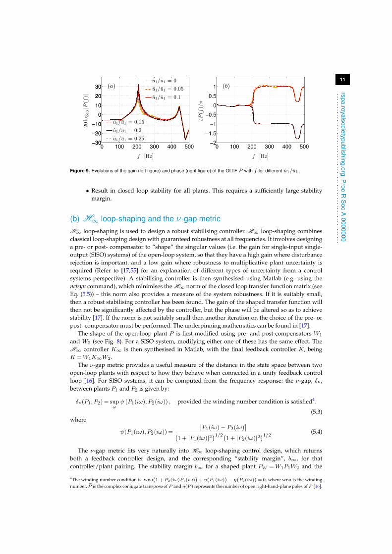
and the time delays corresponding to the microphone position are τ±r = (xr − xf )/(c2 ± u2).Due to the flame nonlinearity, P(s) is nonlinear and depends on u1/u1. Following weakly

nonlinear theory, it can be cast into a set of linear OLTFs, P (s)∈P(s), with a different P (s) foreach value of u1/u1. The OLFTs for different u1/u1 when xf = 0.2 m are shown in Fig. 9.

Each modal peak is associated with a phase change of π, implying a second-order transferfunction contribution. The direction of the phase change provides stability information – a phaseincrease of π corresponds to an unstable conjugate pair of poles while a phase decrease of πindicates a stable conjugate pair. From Fig. 9, normalised velocity perturbation amplitudes, u1/u1,of 0 to 0.15 correspond to unstable OLTFs while amplitudes of 0.2 and 0.25 correspond to stableOLTFs. This is consistent with the previous finding that limit cycle oscillations occur at u1/u1 =

0.18.It is thus clear that a controller design based on just one of these linear OLTFs cannot guarantee

the entire set of plants. In order to guarantee stability from within limit cycle oscillations, a robustcontroller must

• Reduce the size of perturbations when the system is in limit cycle, with the effect ofreducing u1/u1. The set of plants in this regime appear open loop stable.

11

rspa.royalsocietypublishing.orgP

rocR

Soc

A0000000

..........................................................

0 100 200 300 400 500−30

−20

−10

0

10

20

30

f [Hz]

20log 1

0|P

(f)|

u1/u1 = 0

u1/u1 = 0.05

u1/u1 = 0.1

−30

−20

−10

0

10

20

30

u1/u1 = 0.15

u1/u1 = 0.2

u1/u1 = 0.25

(a)

0 100 200 300 400 500−2

−1.5

−1

−0.5

0

0.5

1

f [Hz]

6P(f)/π

(b)

Figure 9. Evolutions of the gain (left figure) and phase (right figure) of the OLTF P with f for different u1/u1.

• Result in closed loop stability for all plants. This requires a sufficiently large stabilitymargin.

(b) H∞ loop-shaping and the ν-gap metricH∞ loop-shaping is used to design a robust stabilising controller. H∞ loop-shaping combinesclassical loop-shaping design with guaranteed robustness at all frequencies. It involves designinga pre- or post- compensator to “shape” the singular values (i.e. the gain for single-input single-output (SISO) systems) of the open-loop system, so that they have a high gain where disturbancerejection is important, and a low gain where robustness to multiplicative plant uncertainty isrequired (Refer to [17,55] for an explanation of different types of uncertainty from a controlsystems perspective). A stabilising controller is then synthesised using Matlab (e.g. using thencfsyn command), which minimises the H∞ norm of the closed loop transfer function matrix (seeEq. (5.5)) – this norm also provides a measure of the system robustness. If it is suitably small,then a robust stabilising controller has been found. The gain of the shaped transfer function willthen not be significantly affected by the controller, but the phase will be altered so as to achievestability [17]. If the norm is not suitably small then another iteration on the choice of the pre- orpost- compensator must be performed. The underpinning mathematics can be found in [17].

The shape of the open-loop plant P is first modified using pre- and post-compensators W1

and W2 (see Fig. 8). For a SISO system, modifying either one of these has the same effect. TheH∞ controller K∞ is then synthesised in Matlab, with the final feedback controller K, beingK =W1K∞W2.

The ν-gap metric provides a useful measure of the distance in the state space between twoopen-loop plants with respect to how they behave when connected in a unity feedback controlloop [16]. For SISO systems, it can be computed from the frequency response: the ν-gap, δν ,between plants P1 and P2 is given by:

δν(P1, P2) = supωψ (P1(iω), P2(iω)) , provided the winding number condition is satisfied4.

(5.3)where

ψ(P1(iω), P2(iω)) =

∣∣P1(iω)− P2(iω)∣∣(

1 + |P1(iω)|2)1/2(

1 + |P2(iω)|2)1/2 (5.4)

The ν-gap metric fits very naturally into H∞ loop-shaping control design, which returnsboth a feedback controller design, and the corresponding “stability margin”, b∞, for thatcontroller/plant pairing. The stability margin b∞ for a shaped plant PW =W1P1W2 and the

4The winding number condition is: wno(1 + P2(iω)P1(iω)

)+ η(P1(iω)

)− η(P2(iω)

)= 0, where wno is the winding

number, P is the complex conjugate transpose ofP and η(P ) represents the number of open right-hand-plane poles ofP [16].

12

rspa.royalsocietypublishing.orgP

rocR

Soc

A0000000

..........................................................

MeanFTFF0(s)

FDFF(u1/u1, s)

Start

MeanOLTFP0(s)

RTF-fittedplantP0F (s)

ChooseW1(s)

All possible OLTFs fordifferent u1/u1: P (s)

Shaped plantP0FW (s)

ν-gap metric:δν(P, P0F )

H∞ loop-shapingsynthesis: ncfsyn

Stabilitymargin:b∞

H∞controller:

K∞

max(δν) > b∞?

averaging over

the FTFs for

u1/u1 ≤ 0.25

+ fitfrd Eq. (5.1)

high cut-off frequency

weighted low-pass

filter + fitfrd

Eq. (5.1)

Yes

No

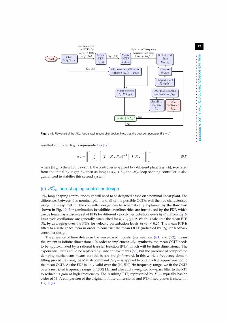
Figure 10. Flowchart of the H∞ loop-shaping controller design. Note that the post-compensator W2 = I .

resulted controller K∞ is represented as [17]:

b∞ =

∥∥∥∥∥[

I

PW

](I −K∞PW )−1

[I K∞

]∥∥∥∥∥−1

∞(5.5)

where ‖·‖∞ is the infinity norm. If the controller is applied to a different plant (e.g. P2), separatedfrom the initial by ν-gap δν , then as long as b∞ > δν , the H∞ loop-shaping controller is alsoguaranteed to stabilise this second system.

(c) H∞ loop-shaping controller designH∞ loop-shaping controller design will need to be designed based on a nominal linear plant. Thedifferences between this nominal plant and all of the possible OLTFs will then be characterisedusing the ν-gap metric. The controller design can be schematically explained by the flowchartshown in Fig. 10. For combustion instabilities, nonlinearities are introduced by the FDF, whichcan be treated as a discrete set of FTFs for different velocity perturbation levels u1/u1. From Fig. 6,limit cycle oscillations are generally established for u1/u1 ≤ 0.2. We thus calculate the mean FTF,F0, by averaging over the FTFs for velocity perturbation levels u1/u1 ≤ 0.25. The mean FTF isfitted to a state space form in order to construct the mean OLTF (indicated by P0) for feedbackcontroller design.

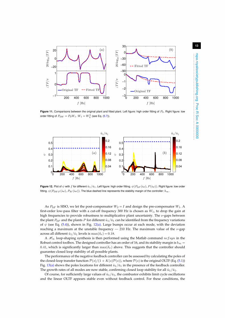
The presence of time delays in the wave-based models, (e.g. see Eqs. (4.1) and (5.2)) meansthe system is infinite dimensional. In order to implement H∞ synthesis, the mean OLTF needsto be approximated by a rational transfer function (RTF) which will be finite dimensional. Theexponential terms could be replaced by Padé approximants [56], but the presence of complicateddamping mechanisms means that this is not straightforward. In this work, a frequency-domainfitting procedure using the Matlab command fitfrd is applied to obtain a RTF approximation tothe mean OLTF. As the FDF is only valid over the [10, 500] Hz frequency range, we fit the OLTFover a restricted frequency range [0, 1000] Hz, and also add a weighted low-pass filter to the RTFto reduce its gain at high frequencies. The resulting RTF, represented by P0F , typically has anorder of 16. A comparison of the original infinite-dimensional and RTF-fitted plants is shown inFig. 11(a).

13

rspa.royalsocietypublishing.orgP

rocR

Soc

A0000000

..........................................................

200 400 600 800 1000−1

0

1

f [Hz]

6TF/π

Original TF

−20

0

20

20log 1

0|T

F|

Fitted TF

(a)

0 200 400 600 800 1000−3

−2

−1

0

f [Hz]

6TF/π

Original TF

−90

−60

−30

0

30

20log 1

0|T

F|

Fitted TF

(b)

Figure 11. Comparisons between the original plant and fitted plant. Left figure: high order fitting of P0. Right figure: low

order fitting of P0W = P0W1. W1 =W 2L (see Eq. (5.7)).

0 200 400 600 800 10000

0.1

0.2

0.3

0.4

0.5

f [Hz]

ψ

u1/u1

0.04

0.08

0.12

0.16

0.2

(a)

0 200 400 600 800 10000

0.1

0.2

0.3

0.4

0.5

f [Hz]

ψ

u1/u1

0.04

0.08

0.12

0.16

0.2

(b)

Figure 12. Plot of ψ with f for different u1/u1. Left figure: high order fitting. ψ(P0F (iω), P (iω)). Right figure: low order

fitting. ψ(P0WF (iω), PW (iω)). The blue dashed line represents the stability margin of the controller: b∞.

As P0F is SISO, we let the post-compensator W2 = I and design the pre-compensator W1. Afirst-order low-pass filter with a cut-off frequency 300 Hz is chosen as W1, to drop the gain athigh frequencies to provide robustness to multiplicative plant uncertainty. The ν-gaps betweenthe plant P0F and the plants P for different u1/u1 can be identified from the frequency variationsof ψ (see Eq. (5.4)), shown in Fig. 12(a). Large bumps occur at each mode, with the deviationreaching a maximum at the unstable frequency — 210 Hz. The maximum value of the ν-gapacross all different u1/u1 levels is max(δν) = 0.18.

A H∞ loop-shaping synthesis is then performed using the Matlab command ncfsyn in theRobust control toolbox. The designed controller has an order of 16, and its stability margin is b∞ =

0.41, which is significantly larger than max(δν) above. This suggests that the controller shouldguarantee closed loop stability of all possible plants.

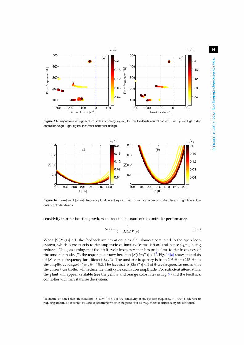
The performance of the negative feedback controller can be assessed by calculating the poles ofthe closed-loop transfer functionP(s)/(1 +K(s)P(s)), whereP(s) is the original OLTF (Eq. (5.1))Fig. 13(a) shows the poles locations for different u1/u1 in the presence of the feedback controller.The growth rates of all modes are now stable, confirming closed loop stability for all u1/u1.

Of course, for sufficiently large values of u1/u1, the combustor exhibits limit cycle oscillationsand the linear OLTF appears stable even without feedback control. For these conditions, the

14

rspa.royalsocietypublishing.orgP

rocR

Soc

A0000000

..........................................................

−300 −200 −100 0 100

100

200

300

400

500

Growth rate [s−1]

Eigenfrequency

[Hz]

u1/u1

0.04

0.08

0.12

0.16

0.2(a)

−300 −200 −100 0 100

100

200

300

400

500

Growth rate [s−1]

Eigenfrequency

[Hz]

u1/u1

0.04

0.08

0.12

0.16

0.2(b)

Figure 13. Trajectories of eigenvalues with increasing u1/u1 for the feedback control system. Left figure: high order

controller deign. Right figure: low order controller design.

190 195 200 205 210 215 2200

0.1

0.2

0.3

0.4

f [Hz]

|S|

u1/u1

0.04

0.08

0.12

0.16

0.2

(a)

190 195 200 205 210 215 2200

0.1

0.2

0.3

0.4

f [Hz]

|S|

u1/u1

0.04

0.08

0.12

0.16

0.2

(b)

Figure 14. Evolution of |S| with frequency for different u1/u1. Left figure: high order controller design. Right figure: low

order controller design.

sensitivity transfer function provides an essential measure of the controller performance.

S(s) =1

1 +K(s)P(s)(5.6)

When |S(i2πf)|< 1, the feedback system attenuates disturbances compared to the open loopsystem, which corresponds to the amplitude of limit cycle oscillations and hence u1/u1 beingreduced. Thus, assuming that the limit cycle frequency matches or is close to the frequency ofthe unstable mode, f?, the requirement now becomes |S(i2πf?)|< 15. Fig. 14(a) shows the plotsof |S| versus frequency for different u1/u1. The unstable frequency is from 205 Hz to 215 Hz inthe amplitude range 0≤ u1/u1 ≤ 0.2. The fact that |S(i2πf?)|< 1 at these frequencies means thatthe current controller will reduce the limit cycle oscillation amplitude. For sufficient attenuation,the plant will appear unstable (see the yellow and orange color lines in Fig. 9) and the feedbackcontroller will then stabilise the system.

5It should be noted that the condition |S(i2πf?)|< 1 is the sensitivity at the specific frequency, f?, that is relevant toreducing amplitude. It cannot be used to determine whether the plant over all frequencies is stabilised by the controller.

15

rspa.royalsocietypublishing.orgP

rocR

Soc

A0000000

..........................................................

0 0.1 0.2 0.3 0.4 0.5

−150

−100

−50

0

50

xf [m]

Growth

rate

[s−1]

u1/u1

Control off

Control on

0.04

0.08

0.12

0.16

0.2

Figure 15. Plot of the growth rate of the unstable mode (f ≈ 210 Hz) with and without control for different flame positions

xf and different velocity perturbation levels u1/u1. The blue dot markers represent the average growth rates.

(d) Low order H∞ loop-shaping controller designIt has been shown that H∞ loop-shaping combined with the ν-gap metric can be used to design arobust controller that guarantees stabilisation from within the limit cycle. The designed controllertypically has an order comparable to that of the shaped plant [55]. High order controllers aredifficult to implement and exhibit lower reliability than low order controllers. Although controllerorder reduction methods, such as balanced truncation methods [57], can be used on the plant orthe controller, this work proposes an alternative approach to directly reduce the order of plant,provided that the maximum ν-gap (max(δν)) is smaller than the stability margin b∞.

The low order method swaps the order of the shaping and fitting procedures. The plant P0 isfirstly shaped with W1 using an “aggressive” low-pass filter, which does not significantly alterthe gain at low frequencies near the unstable mode, but reduces the gain at frequencies abovethe unstable mode, to provide robustness to fitting errors at these frequencies. A low-order fittingprocedure is then implemented on the shaped plant P0W , with the fit over low frequencies nearthe unstable mode prioritised. A fourth order low-pass filter is chosen as the pre-compensatorW1

to shape the original plant, given by W1 =W 2L, where

WL(s) =ω2L

s2 + 2ξLωLs+ ω2L

(5.7)

where ωL = 2π × 200 s−1 and ξL =√

2/2. W1 has a gain of 0.5 at 200 Hz, and so does notsignificantly alter the gain at the unstable frequency. The gain rapidly falls off to 0.025 at 500Hz.

The controller designed by H∞ loop-shaping synthesis generally has a dimension comparableto that of the shaped plant, and so a fitted plant with low dimension is desirable. The shapedsystem contains only one unstable mode and exhibits fast gain fall-off at higher frequencies. Thefitting procedure is performed on the shaped plant P0W = P0W1 — this allows the dimension ofthe fitted RTF to be significantly reduced and yields a RTF is of order of 4. Fig. 11(b) compares theoriginal, P0W , and fitted, P0WF , plants. The fitted RTF captures the shape of original plant at lowfrequencies and has the shape of low-pass filter at high frequencies. Fig. 12(b) shows the evolutionof ψ(P0WF (iω), PW (iω)) with frequency. Compared to the previous approach (Fig. 12(a)), thereare larger deviations at high frequencies (f ≥ 250 Hz) where the low order fitting is less accurate.However, due to the shape ofW1, relatively small values ofψ(P0WF (iω), PW (iω)) are guaranteedfor all frequencies and the maximum of ν-gap for all u1/u1 is max(δν) = 0.34.

A controller with an order of 3 is then obtained from the H∞ loop-shaping synthesis. The finalcontroller K =W1K∞ has an order of 7 in the denominator and 3 in the numerator of its rational

16

rspa.royalsocietypublishing.orgP

rocR

Soc

A0000000

..........................................................

0.1 0.2 0.3 0.4 0.5 0.6 0.7

−0.2

0

0.2

t [s]

u′ 1/u1

−100

0

100

pL[Pa] Control off Control on

Figure 16. Evolution of pL and u′1/u1 with time. The controller is switched on when t= 0.5 s. xf = 0.2 m.

transfer function, which is straightforward to implement. The stability margin is b∞ = 0.52, whichis larger than max (δν).

The locations of the closed-loop poles for different u1/u1 are shown in Fig. 13(b). The unstablemode is stabilised for all u1/u1 and the modes at high frequencies are not disturbed. However,the growth rate reduction for the unstable mode is less than for the high order controller (seeFig. 13(a)). This is due to the larger ν-gap caused by the low order fitting. The gain of thesensitivity function S(s) with frequency is shown in Figure 14(b) and is seen to be smallerthan unity near the unstable mode frequency. This, combined with the fact that b∞ >max (δν),means that the low order controller is also guaranteed to be stabilising from within limit cycleoscillations.

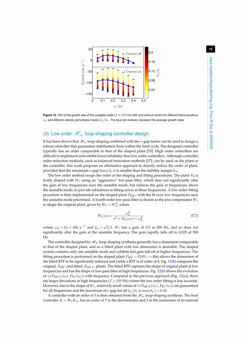
The robustness of the low order controller design to changes in operating condition isinvestigated by moving the flame position along the combustor. Fig. 15 shows that the growthrate of the dominant mode becomes negative for all unstable configurations. Thus the controllerdesigned stabilises all possible flame locations within this combustor.

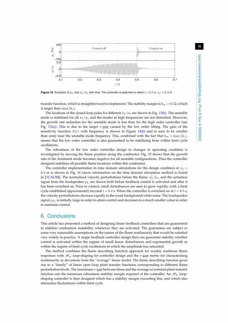
The controller implementation in time domain simulations for the design condition of xf =

0.2 m is shown in Fig. 16 (more information on the time domain simulation method is foundin [31,34,58]). The normalised velocity perturbations before the flame, u′1/u1, and the actuationsignal from the loudspeaker pL are shown both before feedback control is activated and after ithas been switched on. Prior to control, small disturbances are seen to grow rapidly, with a limitcycle established approximately beyond t= 0.4 s. When the controller is switched on at t= 0.5 s,the velocity perturbations decrease rapidly to the weak background white noise. The loudspeakersignal, pL, is initially large in order to attain control and decreases to a much smaller value in orderto maintain control.

6. ConclusionsThis article has presented a method of designing linear feedback controllers that are guaranteedto stabilise combustion instability, whenever they are activated. The guarantees are subject tosome very reasonable assumptions on the nature of the flame nonlinearity that would be satisfiedvery widely in practice. A single feedback controller design then can guarantee stability whethercontrol is activated within the regime of small linear disturbances and exponential growth orwithin the regime of limit cycle oscillations in which the amplitude has saturated.

The method combines the flame describing function approach for weakly nonlinear flameresponses with H∞ loop-shaping for controller design and the ν-gap metric for characterisingnonlinearity as deviations from the “average” linear model. The flame describing function givesrise to a “family” of linear open loop plant transfer functions corresponding to different flameperturbation levels. The maximum ν-gap between these and the average or nominal plant transferfunction sets the minimum robustness stability margin required of the controller. An H∞ loop-shaping controller is then designed which has a stability margin exceeding this, and which alsoattenuates fluctuations within limit cycle.

17

rspa.royalsocietypublishing.orgP

rocR

Soc

A0000000

..........................................................

The control strategy has been demonstrated on a representative model of a nonlinearcombustion system comprising an unsteady laminar flame inside a Rijke tube. Linear planewaves within the duct are assumed to suffer damping due to end radiation and visco-thermalwall damping mechanisms. The nonlinear kinematic response of the flame to flow disturbancesis modelled using a level set approach, which combines the G-equation kinematic flame modelwith a two-dimensional flow velocity perturbation model and a flame front curvature dependentburning speed. Simulations implementing this level set approach have been validated bycomparison with experimental data, and used to determine the flame describing function (FDF)of the laminar conical premixed flame.

The calculated FDF of the target flame has been successfully incorporated into a recentlydeveloped code, OSCILOS, to calculate the eigenvalue evolutions of the nonlinear system withincreasing flame velocity perturbation levels. The corresponding “family” of open loop transferfunctions (OLTF) between the monitored pressure perturbations downstream of the flame andthe external pressure perturbations from an actuator at the entrance of the Rijke tube, has beenestablished for the purpose of control.

A linear mean OLTF has been selected as the target plant for the controller design by averagingthe FDF over a large range of velocity perturbation levels. The ν-gap metric has been applied toquantify the differences between the set of OLTFs for different perturbation levels and the selectedplant. This metric fits naturally into the H∞ loop-shaping framework to provide the minimumrequired stability margin of the designed robust controller. An initial H∞ loop-shaping controllerhas been designed and shown to give effective robust control performance. Subsequently, a loworder H∞ loop-shaping controller based on an aggressively low-pass filtered weighted planthas been designed. Both controllers are guaranteed to stabilise the combustor for all possiblenonlinear flame responses, as long as the ν-gap is smaller than the controller stability margin ofthe controller designed by H∞ loop-shaping synthesis. The resulting controller has been appliedto simulations of the unsteady combustion system in the time domain and has been indeed foundto suppress the combustion instability from within the limit cycle.

Authors’ Contributions. Jingxuan Li and Aimee S. Morgans wrote this article.

Competing Interests. We have no competing interests.

Funding. This work is supported by the European Research Council (ERC) Starting Grant ACOULOMODE(2013-2018).

Appendix

(a) Visco-thermal damping of acoustic waves in a ductThe propagation of sound waves in a duct has been found to be dissipated due to visco-thermallosses at the duct walls [30,59] The forward and backward wavenumbers, k± =−is/c(1±M),are modified to k± = k± +∆k±, where the correction approximately equals:

∆k± =−is1/2

c(1±M

)Λ (A 1)

with the coefficient Λ expressed as:

Λ=2ν1/2

D

(1 +

γ − 1

P1/2r

)(A 2)

where ν and Pr are the kinematic viscosity and Prandtl number of gases, respectively. D is thediameter of the duct. γ is the ratio of specific heats. In the calculation, Pr = 0.71 is consideredconstant, both for air and combustion products of hydro-carbon flames. ν can be calculated byν = µ/ρ, with the dynamic viscosity µair of air calculated by the Sutherland’s Law [60], with

18

rspa.royalsocietypublishing.orgP

rocR

Soc

A0000000

..........................................................

further corrections expressed as:

µair =

µref

(T

Tref

)3/2 Tref + CST + CS

for T ∈ [100, 1000] K

a1T + a0 for T ∈ [1000, 3000] K

where µref = 1.716× 10−5 kg m−1s−1, Tref = 273.15 K, CS = 110.4 K, a1 = 2.653× 10−8 anda0 = 1.573× 10−5. It was found that the dynamic viscosity of the hydrocarbon-air combustionproducts µprod differed little from that of air, with a minor correction depending on theequivalence ratio φ [61], and is written as:

µprod = µair/(1 + 0.027φ), for T ∈ [500, 4000] K, φ∈ [0, 4] (A 3)

The exponential component in propagating waves can be changed to:

exp(±ik±∆x) = exp(∓ τ±(s+ Λs1/2)

)(A 4)

where τ± =∆x/(c± u) and ∆x is the path length of the travelling acoustic wave.

(b) The expressions of Mn

M1 = 1 +S1

S2

(M1(2 +M1

)− c2c1M2(1 +M1

))M3 = 1 +M2

M2 = 1− S1

S2

(M1(2−M1

)− c2c1M2(1−M1

))M4 = 1−M2

M5 = 1 + γM1 + (γ − 1)M21 M7 = 1 + γM2 + (γ − 1)M

22

M6 = 1− γM1 + (γ − 1)M21 M8 = 1− γM2 + (γ − 1)M

22

where M = u/c is the Mach number.

References1. Candel, S., 2002 Combustion dynamics and control: Progress and challenges, P. Combust. Inst.

29, 1–28.2. Lieuwen, T. & Yang, V. (eds.), 2005 Combustion instabilities in gas turbines, Operational experience,

Fundamental mechanisms, and Modeling, volume 210 of Progress in Astronautics and Aeronautics.Reston, Virginia: AIAA, Inc.

3. Chu, B. T., 1964 On the Energy Transfer to Small Disturbances in Fluid Flow (Part I), ActaMechanica 1, 215–234.

4. Dowling, A. P. & Morgans, A. S., 2005 Feedback control of combustion oscillations, Annu. Rev.Fluid Mech. 37, 151–182.

5. Balachandran, R., Ayoola, B. O., Kaminski, C., Dowling, A. P. & Mastorakos, E., 2005Experimental investigation of the nonlinear response of turbulent premixed flames toimposed inlet velocity oscillations, Combust. Flame 143, 37–55.

6. Noiray, N., Durox, D., Schuller, T. & Candel, S., 2008 A unified framework for nonlinearcombustion instability analysis based on the flame describing function., J. Fluid Mech. 615,139–167.

7. Schimek, S., Moeck, J. P. & Paschereit, C. O., 2011 An Experimental Investigation of theNonlinear Response of an Atmospheric Swirl-Stabilized Premixed Flame, J. Eng. Gas TurbinesPower 133, 101502 (7 pages).

8. Harrje, D. T. & Reardon, F. H. (eds.), 1972 Liquid propellant rocket combustion instability.Washington, DC, United States: NASA.

9. Poinsot, T., Veynante, D., Bourienne, F., Candel, S., Esposito, E. & Surget, J., 1989 Initiation andsuppression of combustion instabilities by active control, P. Combust. Inst. 22, 1363–1370.

10. Kabiraj, L. & Sujith, R. I., 2012 Nonlinear self-excited thermoacoustic oscillations:intermittency and flame blowout, J. Fluid Mech. 713, 376–397.

19

rspa.royalsocietypublishing.orgP

rocR

Soc

A0000000

..........................................................

11. Boudy, F., Durox, D., Schuller, T. & Candel, S., 2013 Analysis of limit cycles sustained by twomodes in the flame describing function framework, C.R.Mécanique 341, 181–190.

12. Waugh, I. C., Kashinath, K. & Juniper, M. P., 2014 Matrix-free continuation of limit cycles andtheir bifurcations for a ducted premixed flame, Journal of Fluid Mechanics 759, 1–27.

13. Morgans, A. S. & Dowling, A. P., 2007 Model-based control of combustion instabilities, J.Sound Vib. 299, 261–282.

14. Morgans, A. S. & Stow, S. R., 2007 Model-based control of combustion instabilities in annularcombustors, Comb. and Flame 150, 380–399.

15. Illingworth, S. J. & Morgans, A. S., 2010 Adaptive feedback control of combustion instabilityin annular combustors, Combust. Sci. Technol. 182, 143–164.

16. Vinnicombe, G., 2001 Uncertainty and Feedback: H∞ loop-shaping and the ν-gap metric. London:Imperial College Press.

17. McFarlane, D. & Glover, K., 1992 A loop shaping design procedure using H∞ synthesis, IEEETrans. Autom. Control 37, 759–769.

18. Campos-Delgado, D. U., Schuermans, B. B. H., Zhou, K., Paschereit, C. O., Gallestey, E. A. &Poncet, A., 2003 Thermoacoustic Instabilities: Modeling and Control, IEEE Trans. Control Syst.Technol. 11, 1–15.

19. Chu, Y.-C., Glover, K. & Dowling, A. P., 2003 Control of combustion oscillations via H∞ loop-shaping, µ-analysis and Integral Quadratic Constraints, Automatica 39, 219–231.

20. Yuan, X.-C. & Glover, K., 2013 Model-based control of thermoacoustic instabilities in partiallypremixed lean combustion – a design case study, Int. J. Control 86, 2052–2066.

21. Lauga, E. & Bewley, T., 2004 Performance of a linear robust control strategy on a nonlinearmodel of spatially developing flows, J. Fluid Mech. 512.

22. Weiss, G., Zhong, Q.-C., Green, T. & Liang, J., 2004 H∞ Repetitive Control of DC-ACConverters in Microgrids, IEEE T. Power Electr. 19, 219–230.

23. Lefebvre, D., Chevrel, P. & Richard, S., 2003 An H∞ Based Control Design MethodologyDedicated to the Active Control of Vehicle Longitudinal Oscillations, IEEE Trans. Control Syst.Technol. 11, 948–956.

24. Poinsot, T. & Veynante, D., 2005 Theoretical and Numerical Combustion. Philadelphia,Pennsylvania: R.T. Edwards Inc.

25. Marble, F. E. & Candel, S. M., 1977 Acoustic disturbance from gas non-uniformities convectedthrough a nozzle, J. Sound Vib. 55, 225–243.

26. Lieuwen, T., 2003 Modeling Premixed Combustion-Acoustic Wave Interactions: A Review, J.Propul. Power 19, 765–781.

27. Bourehla, A. & Baillot, F., 1998 Appearance and Stability of a Laminar Conical Premixed FlameSubjected to an Acoustic Perturbation, Combust. Flame 114, 303–318.

28. Dowling, A. P., 1995 The calculation of thermoacoustic oscillations, J. Sound Vib. 180, 557–581.29. Levine, H. & Schwinger, J., 1948 On the radiation of sound from an unflanged circular pipe,

Phys. Rev. 73, 383–406.30. Peters, M., Hirschberg, A., Reijnen, A. & Wijnands, A., 1993 Damping and reflection coefficient

measurements for an open pipe at low Mach and low Helmholtz numbers, J. Fluid Mech. 256,499–534.

31. Li, J. & Morgans, A. S., 2015 Time domain simulations of nonlinear thermoacoustic behaviourin a simple combustor using a wave-based approach, J. Sound Vib. 346, 345–360.

32. Dowling, A. P., 1997 Nonlinear self-excited oscillations of a ducted flame, J. Fluid Mech. 346,271–290.

33. Morgans, A. S. & Annaswamy, A. M., 2008 Adaptive Control of Combustion Instabilities forCombustion Systems with Right-Half Plane Zeros, Combust. Sci. Technol. 180, 1549–1571.

34. Li, J., Yang, D., Luzzato, C. & Morgans, A. S., 2014 OSCILOS: the open sourcecombustion instability low order simulator, Technical report, Imperial College London,http://www.oscilos.com.

35. Han, X., Li, J. & Morgans, A. S., 2015 Prediction of combustion instability limit cycleoscillations by combining flame describing function simulations with a thermoacousticnetwork model, Combust. Flame 162, 3632–3647.

36. Han, X. & Morgans, A. S., 2015 Simulation of the flame describing function of a turbulentpremixed flame using an open-source LES solver, Combust. Flame 162, 1778–1792.

37. Markstein, G., 1964 Nonsteady Flame Propagation. Pergamon Press.38. Dowling, A. P., 1999 A kinematic model of a ducted flame, J. Fluid Mech. 394, 51–72.

20

rspa.royalsocietypublishing.orgP

rocR

Soc

A0000000

..........................................................

39. Luzzato, C. M., Assier, R. C., Morgans, A. S. & Wu, X., 2013 Modelling thermo-acousticinstabilities of an anchored laminar flame in a simple lean premixed combustor: includinghydrodynamic effects, Proc. of the 19th AIAA/CEAS Aeroacoustics Conf. pp. 1–15.

40. Schuller, T., Ducruix, S., Durox, D. & Candel, S., 2002 Modeling tools for the prediction ofpremixed flame transfer functions, P. Combust. Inst. 29, 107–113.

41. Schuller, T., 2003 Mécanismes de Couplage dans les Interactions Acoustique-Combustion, Ph.D.thesis, École Centrale Paris.

42. Kashinath, K., Hemchandra, S. & Juniper, M. P., 2013 Nonlinear thermoacoustics of ductedpremixed flames: The influence of perturbation convection speed, Combust. Flame 160, 2856–2865.

43. Gu, X., Haq, M., Lawes, M. & Woolley, R., 2000 Laminar burning velocity and Marksteinlengths of methane–air mixtures, Combust. Flame 121, 41–58.

44. Li, J., Richecoeur, F. & Schuller, T., 2013 Reconstruction of heat release rate disturbances basedon transmission of ultrasounds: Experiments and modeling for perturbed flames, Combust.Flame 160, 1779–1788.

45. Li, J., Durox, D., Richecoeur, F. & Schuller, T., 2015 Analysis of chemiluminescence, densityand heat release rate fluctuations in acoustically perturbed laminar premixed flames, Combust.Flame 162, 3934–3945.

46. Osher, S. & Fedkiw, R., 2003 Level Set Methods and Dynamic Implicit Surfaces. New York:Springer-Verlag.

47. Gottlieb, S. & Shu, C.-w., 1998 Total variation diminishing Runge-Kutta schemes, Math. Comp.67, 73–85.

48. Peng, D., Merriman, B., Osher, S., Zhao, H. & Kang, M., 1999 A PDE-Based Fast Local LevelSet Method, J. Comput. Phys. 155, 410–438.

49. Wen, X., 2009 High order numerical methods to two dimensional delta function integrals inlevel set methods, J. Comput. Phys. 228, 4273–4290.

50. Durox, D., Schuller, T., Noiray, N. & Candel, S., 2009 Experimental analysis of nonlinear flametransfer functions for different flame geometries, P. Combust. Inst. 32, 1391–1398.

51. Schuller, T., Durox, D. & Candel, S., 2003 A unified model for the prediction of laminar flametransfer functions: comparisons between conical and V-flame dynamics, Combust. Flame 134,21–34.

52. Preetham, Santosh, H. & Lieuwen, T., 2008 Dynamics of Laminar Premixed Flames Forced byHarmonicVelocity Disturbances, J. Propul. Power 24, 1390–1402.

53. Raun, R. L., Beckstead, M. W., Finlinson, J. C. & Brooks, K. P., 1993 A review of Rijke tubes,Rijke burners and related devices, Prog. Energ. Combust. 19, 313–364.

54. Evesque, S., Dowling, A. P. & Annaswamy, A. M., 2003 Self-tuning regulators for combustionoscillations, Proc. R. Soc. Lond. A 459, 1709–1749.

55. Zhou, K., C.Doyle, J. & Glover, K., 1996 Robust and Optimal Control. New Jersey: Prentice-Hall.56. Brezinski, C., 1996 Extrapolation algorithms and Padé approximations: a historical survey,

Appl. Numer. Math. 20, 299–318.57. Gugercin, S. & Antoulas, A. C., 2004 A Survey of Model Reduction by Balanced Truncation

and Some New Results, Int. J. Control 77, 748–766.58. Li, J. & Morgans, A. S., 2014 Model based control of nonlinear combustion instabilities, In The

21st International Congress on Sound and Vibration. Beijing.59. Kirchhoff, G., 1868 Uber den einfluss der wärmteleitung in einem gas auf die schallbewegung,

Annalen der Physik 134, 177–193.60. Sutherland, W., 1893 The viscosity of gases and molecular force, Philosophical Magazine Series

5 36, 507–531.61. Mansouri, S. H. & Heywood, J. B., 1980 Correlations for the Viscosity and Prandtl Number of

Hydrocarbon-Air Combustion Products, Combust. Sci. Technol. 23, 251–256.