Rosenbrock Methods€¦ · 3 = 5:000000000000e 01 ^b 3 = 1:388888888888e 01 Table:ROS3w (with a...
22
Outline Introduction Stability Order conditions Computational results End Rosenbrock Methods Yue Yu December 9, 2009 Yue Yu Rosenbrock Methods
Transcript of Rosenbrock Methods€¦ · 3 = 5:000000000000e 01 ^b 3 = 1:388888888888e 01 Table:ROS3w (with a...
OutlineIntroduction
StabilityOrder conditions
Computational resultsEnd
Rosenbrock Methods
Yue Yu
December 9, 2009
Yue Yu Rosenbrock Methods

OutlineIntroduction
StabilityOrder conditions
Computational resultsEnd
IntroductionInspirationspecial cases
StabilityA-stability and L-stability
Order conditionsRooted treesγii = γW-methods
Computational resultsComputational efficiency
EndConclusionReferences
Yue Yu Rosenbrock Methods
OutlineIntroduction
StabilityOrder conditions
Computational resultsEnd
Inspirationspecial cases
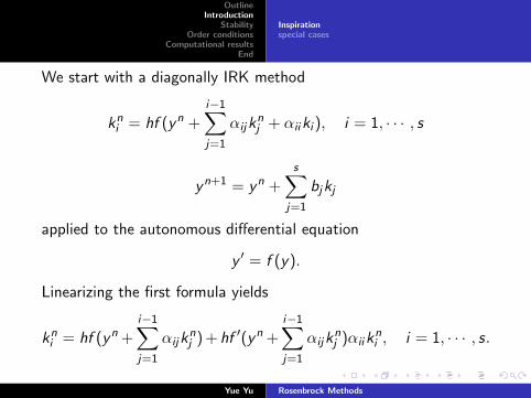
We start with a diagonally IRK method
kni = hf (yn +
i−1∑j=1
αijknj + αiiki ), i = 1, · · · , s
yn+1 = yn +s∑
j=1
bjkj
applied to the autonomous differential equation
y ′ = f (y).
Linearizing the first formula yields
kni = hf (yn +
i−1∑j=1
αijknj ) + hf ′(yn +
i−1∑j=1
αijknj )αiik
ni , i = 1, · · · , s.
Yue Yu Rosenbrock Methods
OutlineIntroduction
StabilityOrder conditions
Computational resultsEnd
Inspirationspecial cases
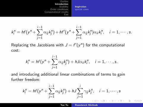
kni = hf (yn +
i−1∑j=1
αijknj ) + hf ′(yn +
i−1∑j=1
αijknj )αiik
ni , i = 1, · · · , s.
Replacing the Jacobians with J = f ′(yn) for the computationalcost:
kni = hf (yn +
i−1∑j=1
αijknj ) + hJαiik
ni , i = 1, · · · , s.
and introducing additional linear combinations of terms to gainfurther freedom:
kni = hf (yn +
i−1∑j=1
αijknj ) + hJ
i∑j=1
γijknj , i = 1, · · · , s
Yue Yu Rosenbrock Methods
OutlineIntroduction
StabilityOrder conditions
Computational resultsEnd
Inspirationspecial cases
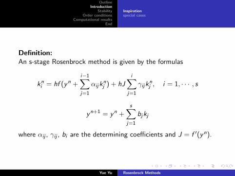
Definition:An s-stage Rosenbrock method is given by the formulas
kni = hf (yn +
i−1∑j=1
αijknj ) + hJ
i∑j=1
γijknj , i = 1, · · · , s
yn+1 = yn +s∑
j=1
bjkj
where αij , γij , bi are the determining coefficients and J = f ′(yn).
Yue Yu Rosenbrock Methods
OutlineIntroduction
StabilityOrder conditions
Computational resultsEnd
Inspirationspecial cases
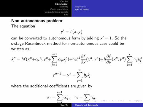
Non-autonomous problem:The equation
y ′ = f (x , y)
can be converted to autonomous form by adding x ′ = 1. So thes-stage Rosenbrock method for non-autonomous case could bewritten as
kni = hf (xn+αih, y
n+i−1∑j=1
αijknj )+γih
2 ∂f
∂x(xn, yn)+h
∂f
∂y(xn, yn)
i∑j=1
γijknj
yn+1 = yn +s∑
j=1
bjkj
where the additional coefficients are given by
αi =i−1∑j=1
αij , γi =i∑
j=1
γij .
Yue Yu Rosenbrock Methods
OutlineIntroduction
StabilityOrder conditions
Computational resultsEnd
Inspirationspecial cases
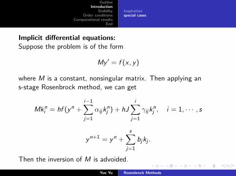
Implicit differential equations:Suppose the problem is of the form
My ′ = f (x , y)
where M is a constant, nonsingular matrix. Then applying ans-stage Rosenbrock method, we can get
Mkni = hf (yn +
i−1∑j=1
αijknj ) + hJ
i∑j=1
γijknj , i = 1, · · · , s
yn+1 = yn +s∑
j=1
bjkj .
Then the inversion of M is advoided.
Yue Yu Rosenbrock Methods
OutlineIntroduction
StabilityOrder conditions
Computational resultsEnd
A-stability and L-stability
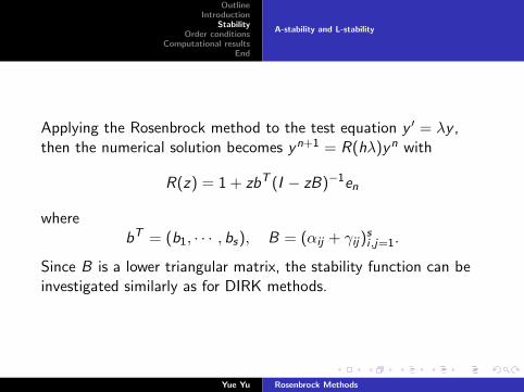
Applying the Rosenbrock method to the test equation y ′ = λy ,then the numerical solution becomes yn+1 = R(hλ)yn with
R(z) = 1 + zbT (I − zB)−1en
wherebT = (b1, · · · , bs), B = (αij + γij)
si ,j=1.
Since B is a lower triangular matrix, the stability function can beinvestigated similarly as for DIRK methods.
Yue Yu Rosenbrock Methods
OutlineIntroduction
StabilityOrder conditions
Computational resultsEnd
A-stability and L-stability
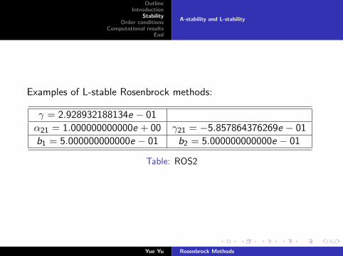
Examples of L-stable Rosenbrock methods:
γ = 2.928932188134e − 01
α21 = 1.000000000000e + 00 γ21 = −5.857864376269e − 01
b1 = 5.000000000000e − 01 b2 = 5.000000000000e − 01
Table: ROS2
Yue Yu Rosenbrock Methods
OutlineIntroduction
StabilityOrder conditions
Computational resultsEnd
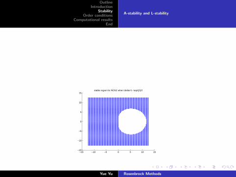
A-stability and L-stability
−15 −10 −5 0 5 10 15−15
−10
−5
0
5
10
15stable region for ROS2 when \delta=1−\sqrt{2}/2
Figure: stablity region for ROS2 scheme
Yue Yu Rosenbrock Methods
OutlineIntroduction
StabilityOrder conditions
Computational resultsEnd
A-stability and L-stability
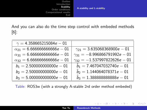
And you can also do the time step control with embeded methods[6]:
γ = 4.358665215084e − 01
α21 = 6.666666666666e − 01 γ21 = 3.635068368900e − 01α31 = 6.666666666666e − 01 γ31 = −8.996866791992e − 01α32 = 6.666666666666e − 01 γ32 = −1.537997822626e − 01
b1 = 2.500000000000e − 01 b̂1 = 7.467047032740e − 01
b2 = 2.500000000000e − 01 b̂2 = 1.144064078371e − 01
b3 = 5.000000000000e − 01 b̂3 = 1.388888888888e − 01
Table: ROS3w (with a strongly A-stable 2rd order method embeded)
Yue Yu Rosenbrock Methods
OutlineIntroduction
StabilityOrder conditions
Computational resultsEnd
Rooted treesγii = γW-methods
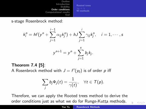
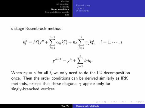
s-stage Rosenbrock method:
kni = hf (yn +
i−1∑j=1
αijknj ) + hJ
i∑j=1
γijknj , i = 1, · · · , s
yn+1 = yn +s∑
j=1
bjkj .
Theorem 7.4 [5]:A Rosenbrock method with J = f ′(y0) is of order p iff∑
j
bjΦj(t) =1
γ(t), ∀t ∈ T (p).
Therefore, we can apply the Rooted trees method to derive theorder conditions just as what we do for Runge-Kutta methods.
Yue Yu Rosenbrock Methods
OutlineIntroduction
StabilityOrder conditions
Computational resultsEnd
Rooted treesγii = γW-methods
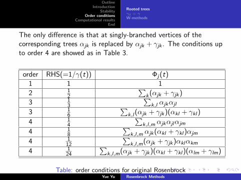
The only difference is that at singly-branched vertices of thecorresponding trees αjk is replaced by αjk + γjk . The conditions upto order 4 are showed as in Table 3.
order RHS(=1/γ(t)) Φj(t)
1 1 1
2 12
∑k(αjk + γjk)
3 13
∑k,l αjkαjl
3 16
∑k,l(αjk + γjk)(αkl + γkl)
4 14
∑k,l ,m αjkαjlαjm
4 18
∑k,l ,m αjk(αkl + γkl)αjm
4 112
∑k,l ,m(αjk + γjk)αklαkm
4 124
∑k,l ,m(αjk + γjk)(αkl + γkl)(αlm + γlm)
Table: order conditions for original RosenbrockYue Yu Rosenbrock Methods
OutlineIntroduction
StabilityOrder conditions
Computational resultsEnd
Rooted treesγii = γW-methods
s-stage Rosenbrock method:
kni = hf (yn +
i−1∑j=1
αijknj ) + hJ
i∑j=1
γijknj , i = 1, · · · , s
yn+1 = yn +s∑
j=1
bjkj .
When γii = γ for all i , we only need to do the LU decompositiononce. Then the order conditions can be derived similarly as IRKmethods, except that these diagonal γ appear only forsingly-branched vertices.
Yue Yu Rosenbrock Methods
OutlineIntroduction
StabilityOrder conditions
Computational resultsEnd
Rooted treesγii = γW-methods
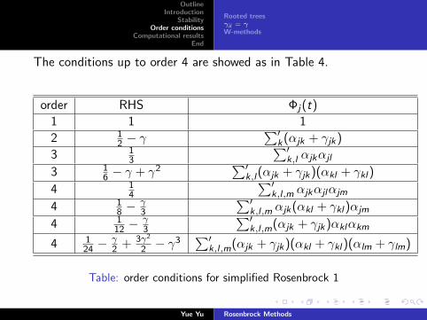
The conditions up to order 4 are showed as in Table 4.
order RHS Φj(t)
1 1 1
2 12 − γ
∑′k(αjk + γjk)
3 13
∑′k,l αjkαjl
3 16 − γ + γ2
∑′k,l(αjk + γjk)(αkl + γkl)
4 14
∑′k,l ,m αjkαjlαjm
4 18 −
γ3
∑′k,l ,m αjk(αkl + γkl)αjm
4 112 −
γ3
∑′k,l ,m(αjk + γjk)αklαkm
4 124 −
γ2 + 3γ2
2 − γ3
∑′k,l ,m(αjk + γjk)(αkl + γkl)(αlm + γlm)
Table: order conditions for simplified Rosenbrock 1
Yue Yu Rosenbrock Methods
OutlineIntroduction
StabilityOrder conditions
Computational resultsEnd
Rooted treesγii = γW-methods
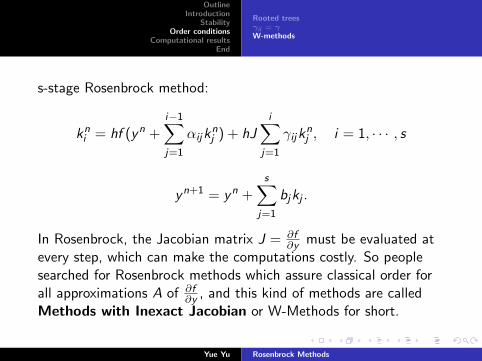
s-stage Rosenbrock method:
kni = hf (yn +
i−1∑j=1
αijknj ) + hJ
i∑j=1
γijknj , i = 1, · · · , s
yn+1 = yn +s∑
j=1
bjkj .
In Rosenbrock, the Jacobian matrix J = ∂f∂y must be evaluated at
every step, which can make the computations costly. So peoplesearched for Rosenbrock methods which assure classical order forall approximations A of ∂f
∂y , and this kind of methods are calledMethods with Inexact Jacobian or W-Methods for short.
Yue Yu Rosenbrock Methods
OutlineIntroduction
StabilityOrder conditions
Computational resultsEnd
Rooted treesγii = γW-methods
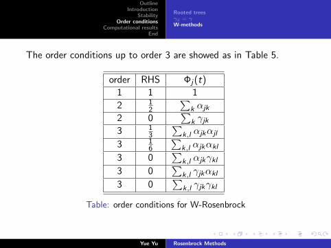
The order conditions up to order 3 are showed as in Table 5.
order RHS Φj(t)
1 1 1
2 12
∑k αjk
2 0∑
k γjk
3 13
∑k,l αjkαjl
3 16
∑k,l αjkαkl
3 0∑
k,l αjkγkl
3 0∑
k,l γjkαkl
3 0∑
k,l γjkγkl
Table: order conditions for W-Rosenbrock
Yue Yu Rosenbrock Methods
OutlineIntroduction
StabilityOrder conditions
Computational resultsEnd
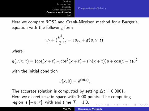
Computational efficiency
Here we compare ROS2 and Crank-Nicolson method for a Burger’sequation with the following form
ut + (u2
2)x = εuxx + g(u, x , t)
where
g(u, x , t) = (cos(x + t)− cos2(x + t) + sin(x + t))u + cos(x + t)u2
with the initial condition
u(x , 0) = esin(x).
The accurate solution is computted by setting ∆t = 0.0001.Here we discretize u in space with 1000 points. The computingregion is [−π, π], with end time T = 1.0.
Yue Yu Rosenbrock Methods
OutlineIntroduction
StabilityOrder conditions
Computational resultsEnd
Computational efficiency
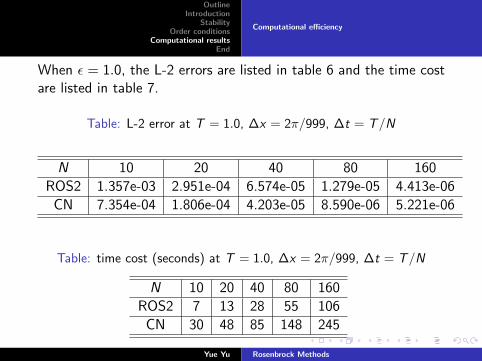
When ε = 1.0, the L-2 errors are listed in table 6 and the time costare listed in table 7.
Table: L-2 error at T = 1.0, ∆x = 2π/999, ∆t = T/N
N 10 20 40 80 160
ROS2 1.357e-03 2.951e-04 6.574e-05 1.279e-05 4.413e-06
CN 7.354e-04 1.806e-04 4.203e-05 8.590e-06 5.221e-06
Table: time cost (seconds) at T = 1.0, ∆x = 2π/999, ∆t = T/N
N 10 20 40 80 160
ROS2 7 13 28 55 106
CN 30 48 85 148 245
Yue Yu Rosenbrock Methods
OutlineIntroduction
StabilityOrder conditions
Computational resultsEnd
ConclusionReferences
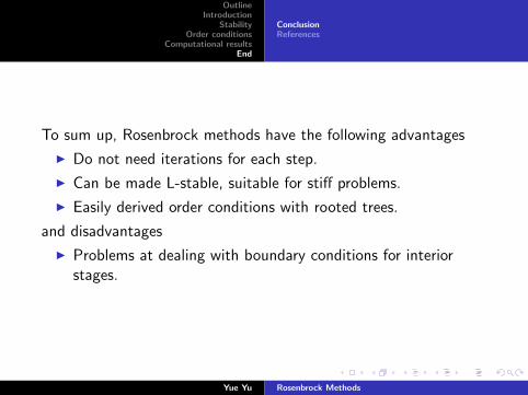
To sum up, Rosenbrock methods have the following advantages
I Do not need iterations for each step.
I Can be made L-stable, suitable for stiff problems.
I Easily derived order conditions with rooted trees.
and disadvantages
I Problems at dealing with boundary conditions for interiorstages.
Yue Yu Rosenbrock Methods
OutlineIntroduction
StabilityOrder conditions
Computational resultsEnd
ConclusionReferences
I H.H. Rosenbrock, Some general implicit processes for thenumerical solution of differential equations, Comput. J. , 5,329330, 1963.
I J.G. Verwer, An analysis of Rosenbrock methods for nonlinearstiff initial value problems, SIAM J. Numer. Anal. 19,155-170, 1982.
I J.G. Verwer, Instructive experiments with someRunge-Kutta-Rosenbrock methods, Comp. and Math. withAppls. 7, 217-229, 1982.
I J.G. Verwer, S. Scholz, J.G. Blom and M. Louter-Nool, Aclass of Runge-Kutta-Rosenbrock methods for stiff differentialequations, ZAMM 63, 13-20, 1983.
Yue Yu Rosenbrock Methods
OutlineIntroduction
StabilityOrder conditions
Computational resultsEnd
ConclusionReferences
I E. Hairer and G. Wanner, Solving Ordinary DifferentialEquations II: Stiff and Differential-Algebraic Equations,Springer Series in Computational Mathematics 14, SpringerVerlag, 2nd edition, 1996.
I J.Rang and L.Angermann, New Rosenbrock W-Methods ofOrder 3 for Partial Differentail Algebraic Equations of Index 1,BIT Numerical Mathematics 45, 761-787, 2005.
Yue Yu Rosenbrock Methods