
Risk-averse Capital Market Line using Revised Option … Portfolio Insurance ... free asset is not...
28
Author: Rachid Bouchaib ICA 2006 Paris Risk-averse Capital Market Line using Revised Option-Based Portfolio Insurance Abstract Selecting a complete portfolio from Capital Market Line (CML) is the main asset allocation decision in efficient portfolio theory. A review of the literature reveals a lack of methodology, which can be used in practice to achieve a balance between investing in the risky portfolio and the risk-free asset. This has been a major challenge for many financial institutions such as insurance and pension funds especially in the aftermath of one of the most volatile periods in recent financial history. This article develops a methodology governing complete portfolio and CML construction based on a downside-risk framework using option pricing theory. Revised Option-based Portfolio Insurance (ROBPI) is a dynamic asset allocation process designed to maximise risky asset exposure with a downside protection. Linking ROBPI to efficient diversification theory leads to Risk- averse Capital Market Line function (RCML) assisting complete portfolios selection from CMLs depending on three parameters: risk aversion measure, risky asset volatility and duration of the investment period. An earlier version of this paper, Dynamic Asset Allocation To Hedge Cash Guarantees using Revised Option-Based Portfolio Insurance, was presented to the 2004 Finance & Investment Conference organised by the British Institute of Actuaries in Brussels. KEYWORDS Portfolio Insurance, replicating portfolio, synthetic options, efficient frontier, the optimal risky portfolio, Capital Market Line CONTACT DETAILS AVIVA Limited 4 Shenton Way # 01-01 SGX Centre 2 Singapore 068807 DID (65) 6827 7536 Fax: (65) 6827 7568 Mobile: (65) 9337 3370 Email: [email protected] I Rachid Bouchaib certify that this article contains my personal views and research. This article and the opinions contained within are for the internal use of the scientific committee of ICA 2006 Paris. Distribution or disclosure of this draft article to any other party is prohibited without the prior consent of the author. Opinions expressed are not necessarily those of my employer, any errors remain my own. Page 1 of 28 Risk-averse Capital Market Line (1st Draft) Author: Rachid Bouchaib
Transcript of Risk-averse Capital Market Line using Revised Option … Portfolio Insurance ... free asset is not...
Author: Rachid Bouchaib ICA 2006 Paris
Risk-averse Capital Market Line
using Revised Option-Based Portfolio Insurance
Abstract Selecting a complete portfolio from Capital Market Line (CML) is the main asset allocation decision in efficient portfolio theory. A review of the literature reveals a lack of methodology, which can be used in practice to achieve a balance between investing in the risky portfolio and the risk-free asset. This has been a major challenge for many financial institutions such as insurance and pension funds especially in the aftermath of one of the most volatile periods in recent financial history. This article develops a methodology governing complete portfolio and CML construction based on a downside-risk framework using option pricing theory. Revised Option-based Portfolio Insurance (ROBPI) is a dynamic asset allocation process designed to maximise risky asset exposure with a downside protection. Linking ROBPI to efficient diversification theory leads to Risk-averse Capital Market Line function (RCML) assisting complete portfolios selection from CMLs depending on three parameters: risk aversion measure, risky asset volatility and duration of the investment period.
An earlier version of this paper, Dynamic Asset Allocation To Hedge Cash Guarantees using Revised Option-Based Portfolio Insurance, was presented to the 2004 Finance & Investment Conference organised by the British Institute of Actuaries in Brussels.
KEYWORDS
Portfolio Insurance, replicating portfolio, synthetic options, efficient frontier, the optimal risky portfolio, Capital Market Line
CONTACT DETAILS
AVIVA Limited 4 Shenton Way # 01-01 SGX Centre 2 Singapore 068807 DID (65) 6827 7536 Fax: (65) 6827 7568 Mobile: (65) 9337 3370 Email: [email protected] I Rachid Bouchaib certify that this article contains my personal views and research. This article and the opinions contained within are for the internal use of the scientific committee of ICA 2006 Paris. Distribution or disclosure of this draft article to any other party is prohibited without the prior consent of the author. Opinions expressed are not necessarily those of my employer, any errors remain my own.
Page 1 of 28 Risk-averse Capital Market Line (1st Draft) Author: Rachid Bouchaib
1 Introduction Option-Based Portfolio Insurance (OBPI) is an investment strategy, which combines conventional assets and vanilla options, aiming to achieve a diversified risky portfolio exposure and to protect the investment over a certain period. The following two investment strategies define OBPI as outlined in portfolio management literature:
• Hold a diversified risky portfolio and buy a Put option • Hold risk-free assets and buy a Call option
OBPI based on a Put approach is usually expressed as follows
PutSV +=
Where • is the total value of a portfolio V• is a diversified risky portfolio S• Put is a European put option on S with maturity T and strike K • K is the floor representing the targeted minimum value of V at maturity • T is the investment period of the portfolio insurance
It is assumed throughout this article that S is the optimal risky portfolio following Markowitz’s approach (1952, 1958). Any dividends from risky assets are assumed to be reinvested within the portfolio. The equivalent strategy based on Call approach can be expressed as follows
CallZCV +=
Where • ZC is a risk-free zero coupon bond such as and r is the risk-free rate TreKZC ⋅−⋅=• Call is a European call option on S with maturity T and strike K
The formulation of OBPI was first introduced by Leland & Rubinstein (1976). Its popularity among insurance and pension funds has been very limited, as it cannot be applied in practice without extra funding. The value of an existing portfolio is not necessarily equal to the price of a zero-coupon bond and a long position in a single Call option. Therefore, Put formulation is also incomplete and it will be shown that a self-funded OBPI using Put strategy requires a long position in the risky asset, risk-free bonds, and a Put option. Revised Option-Based Portfolio Insurance (ROBPI) is a self-funded version of OBPI. Replicating underlying options of self-funded OBPI by investing only in the risky portfolio and risk-free bonds leads to a dynamic capital allocation process. Linking ROBPI results to portfolio theory leads to Risk-averse Capital Market Line function (RCML). Combining the level of risk-free exposure given by RCML function with Markowitz’s optimal risky portfolio gives all possible complete portfolios and Capital Market Lines depending on Risk Averse Measure, risky asset volatility and the investment period. Unlike systematic portfolio technique, severely criticised in the 1987 market crash, RCML function is designed to help investors assessing the downside-risk expressed as Risk Averse Measure (RAM) related to asset allocation decisions. For instance, RCML with a fixed Risk Averse Measure leads to risky asset exposure that increases with the passage of time regardless of market movements.
Page 2 of 28 Risk-averse Capital Market Line (1st Draft) Author: Rachid Bouchaib
2 Revised Option-Based Portfolio Insurance 2.1 ROBPI using traded options There are three stages in the development of the analytical formula of RCML function. The first step is to establish ROBPI formulation using a Call option. The appropriate formulation of a self-funded OBPI using a traded Call option reflecting market cost is as follows
CallZCV ⋅+= λ
Where • is Black & Scholes (1973) Call option price priceCall
• Lambda is a Call proportion such as +
−=
priceCallZCVλ ( ) ( )
+
⋅−⋅
−=
ZCdNdNVZCV
21
•
( ) ( )
( )tT
tTBZC
V
d t
t
−⋅
−⋅+
⋅
=σ
σ2ln
2
1
• ( )tTdd −⋅−= σ12 • σ is the implied volatility of the risky portfolio • is the normal distribution. ( ).N
Lambda is a Call proportion that makes OBPI self-funded. After investing in a risk-free bond to provide the floor, remaining assets are invested in a Call option to provide participation in risky portfolio growth. The risky asset is a non-dividend paying portfolio implying that the value of Call proportion is always between zero and one, which is a feature of Black & Scholes’ (1973) Call option formula. Put formulation
ROBPI using a Put option can be derived from a Call formulation by using Call-Put parity. Replacing the Call option by its equivalent Put option structure gives the following portfolio
ZCPutSV ⋅−++⋅= )1()( λλ
This portfolio indicates that an equity portfolio aiming to achieve self-funded OBPI by purchasing a Put option should also invest in a risk-free bond. Liquidating some of the risky assets to purchase a Put option is not sufficient to provide the required protection. Call and Put option strategies are equivalent, but Call option strategy is the focus of this article. It provides a direct and general ROBPI formula by using a Call spread strategy instead of a Call option.
Page 3 of 28 Risk-averse Capital Market Line (1st Draft) Author: Rachid Bouchaib
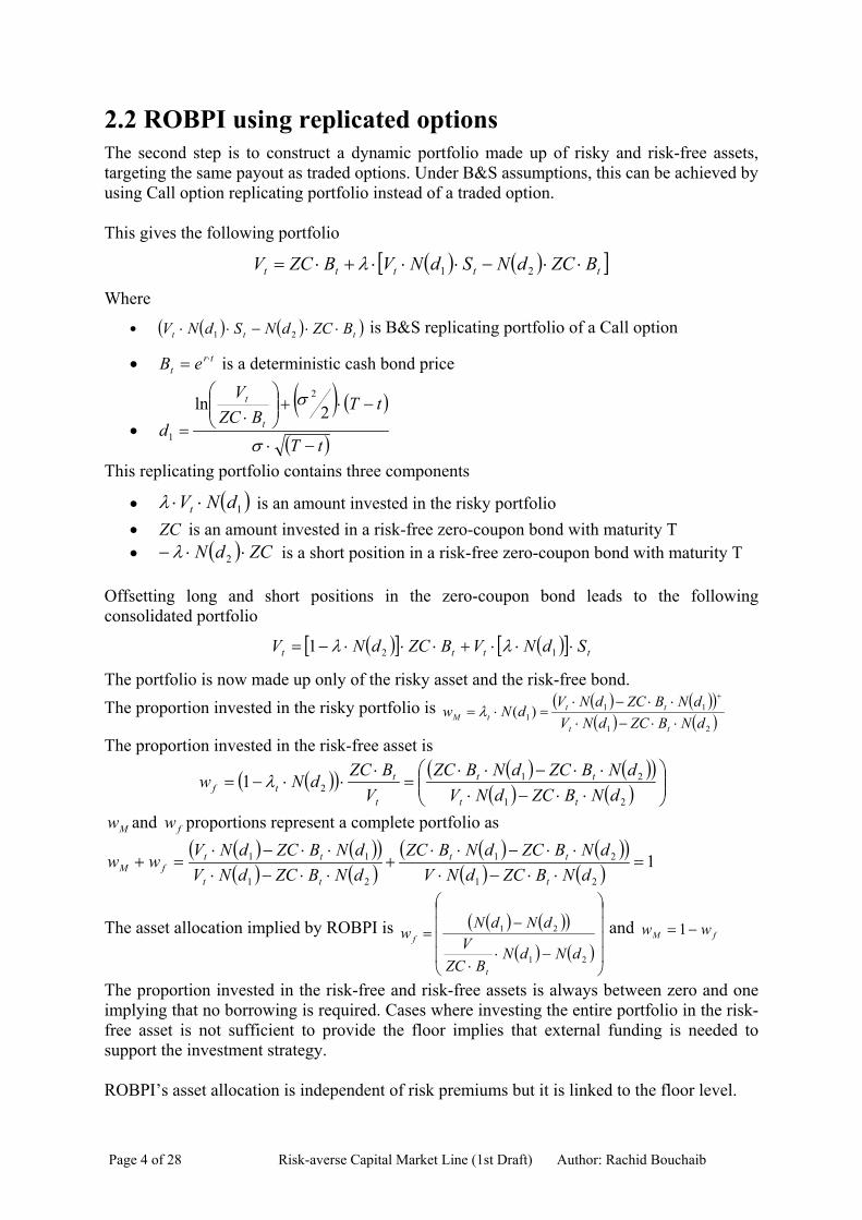
2.2 ROBPI using replicated options The second step is to construct a dynamic portfolio made up of risky and risk-free assets, targeting the same payout as traded options. Under B&S assumptions, this can be achieved by using Call option replicating portfolio instead of a traded option. This gives the following portfolio
( ) ( )[ ]ttttt BZCdNSdNVBZCV ⋅⋅−⋅⋅⋅+⋅= 21λ Where
• ( ) ( )( ttt BZCdNSdNV ⋅⋅−⋅⋅ 21 ) is B&S replicating portfolio of a Call option
• is a deterministic cash bond price trt eB ⋅=
•
( ) ( )
( )tT
tTBZC
V
d t
t
−⋅
−⋅+
⋅
=σ
σ2ln
2
1
This replicating portfolio contains three components
• ( 1dNVt ⋅⋅ )λ is an amount invested in the risky portfolio • is an amount invested in a risk-free zero-coupon bond with maturity T ZC• ( ) ZCdN ⋅⋅− 2λ is a short position in a risk-free zero-coupon bond with maturity T
Offsetting long and short positions in the zero-coupon bond leads to the following consolidated portfolio
( )[ ] ( )[ ] tttt SdNVBZCdNV ⋅⋅⋅+⋅⋅⋅−= 121 λλ
The portfolio is now made up only of the risky asset and the risk-free bond. The proportion invested in the risky portfolio is ( ) ( )( )
( ) ( )21
111 )(
dNBZCdNVdNBZCdNV
dNwtt
tttM ⋅⋅−⋅
⋅⋅−⋅=⋅=
+
λ
The proportion invested in the risk-free asset is
( )( ) ( ) ( )( )( ) ( )
⋅⋅−⋅
⋅⋅−⋅⋅=
⋅⋅⋅−=
21
2121
dNBZCdNVdNBZCdNBZC
VBZC
dNwtt
tt
t
ttf λ
Mw and proportions represent a complete portfolio as fw( ) ( )( )( ) ( )
( ) ( )( )( ) ( ) 1
21
21
21
11 =⋅⋅−⋅
⋅⋅−⋅⋅+
⋅⋅−⋅⋅⋅−⋅
=+dNBZCdNV
dNBZCdNBZCdNBZCdNVdNBZCdNV
wwt
tt
tt
ttfM
The asset allocation implied by ROBPI is ( ) ( )( )( ) ( )
−⋅⋅
−=
21
21
dNdNBZC
VdNdN
w
t
f and fM ww −= 1
The proportion invested in the risk-free and risk-free assets is always between zero and one implying that no borrowing is required. Cases where investing the entire portfolio in the risk-free asset is not sufficient to provide the floor implies that external funding is needed to support the investment strategy. ROBPI’s asset allocation is independent of risk premiums but it is linked to the floor level.
Page 4 of 28 Risk-averse Capital Market Line (1st Draft) Author: Rachid Bouchaib
2.3 Numerical illustrations The following table shows numerical examples of risky portfolio exposure using ROBPI formula with different floors and investment periods. These examples are for illustration purposes only as they are based on 20% risky asset volatility and a risk-free rate of 4%.
Time horizon Floor as % 3-Year 4-Year 5-Year 6-Year 7-Year 8-Year 9-Year 10-Year
90% 64% 65% 67% 69% 70% 72% 74% 75% 95% 53% 56% 59% 62% 64% 67% 69% 71% 100% 40% 46% 50% 54% 57% 61% 63% 66% 105% 25% 34% 40% 46% 50% 54% 57% 61% 110% 9% 21% 29% 36% 42% 47% 51% 55%
Table 1: Risky portfolio exposure based on a Call option Risky asset exposures increase with the investment period and decrease with floors. Using a normal shape of volatility term-structure of an equity index makes risky asset exposure less sensitive to the floor level, especially for long-dated investment periods. ROBPI using Call spread strategy As mentioned earlier, Call spread is a more general form of Call option strategies. Using Call derive ROBPI formula leads to a reduced risky asset exposure. The ROBPI formula represents the risk-free asset exposure using Call spread strategy for 0=t
( ) ( )( ) ( ) ( )( )( ) ( ) ( ) ( )
⋅−⋅
⋅⋅−−⋅
⋅
⋅−⋅−−=
ββ
ββ
βα
βα
2121
2121
dNdNBZC
VdNdNBZC
VdNdNdNdN
w
tt
f
Where • α is a positive Call spread proportion with a value between 0 and 1. • are the strikes of the Call spread 21 and KK• β is a positive parameter such as β⋅= 12 KK and 1≥β • are based on strike 21 and dd 1K• are based on strike ββ
21 and dd β⋅1K
The following table shows risky asset exposure based on Call spread with 5.1=β and 1=α Time horizon
Floor =K / V 3-Year 4-Year 5-Year 6-Year 7-Year 8-Year 9-Year 10-Year 90% 49% 47% 46% 45% 45% 45% 44% 44% 95% 42% 42% 42% 43% 43% 43% 43% 43% 100% 33% 36% 37% 39% 40% 40% 41% 41% 105% 22% 27% 31% 34% 36% 37% 38% 39% 110% 8% 17% 23% 28% 31% 33% 35% 37%
Table 2: Risky portfolio exposure for using a Call spread based
ROBPI based on Call spread strategy gives a lower initial risky asset exposure than Call option strategy especially for low floors. Call spread strategy combined with long-dated investment period gives risky asset exposures, which converge towards the same value regardless of floor levels.
Page 5 of 28 Risk-averse Capital Market Line (1st Draft) Author: Rachid Bouchaib
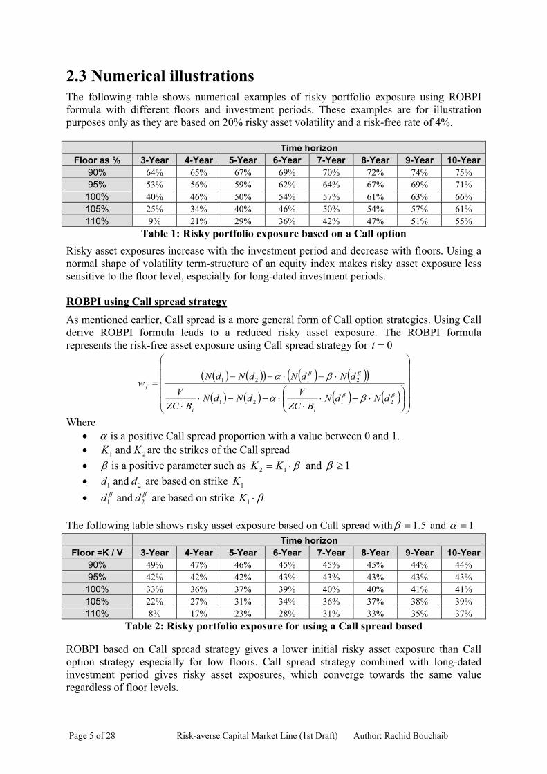
2.4 Past performance The following figure illustrates the past performance of a dynamic asset allocation between the risk-free asset and FTSE All-shares using ROBPI formula. Any other risky portfolios including dividend income in their performance such as DAX equity index can be used to assess the past performance of ROBPI formula. Assumptions for this analysis are:
• 150% is a minimum maturity payout • The investment period started in Feb 1994 and ended in Feb 2004 • 6% is the risk-free rate over the period • Monthly rebalancing of asset allocation with 15% minimum switch trigger for
smoothed strategy • No tax or transaction cost
Past performance of dynamic capital allocation(10-year investment period with 150% floor maturing in Feb 2004)
0%
20%
40%
60%
80%
100%
120%
140%
160%
180%
200%
02/9408/94
02/9508/95
02/9608/96
02/9708/97
02/9808/98
02/9908/99
02/0008/00
02/0108/01
02/0208/02
02/0308/03
0%
20%
40%
60%
80%
100%
120%
140%
160%
180%
200%
FTSE exposure (smoothed ROBPI) ROBPI performance FTSE All-Share FTSE exposure (ROBPI)
Figure 1: ROBPI targeting 150% maturity payout
The chart shows that the floor is met despite a 23% FTSE all-share delivered volatility during this period. The objective of ROBPI is to protect the initial investment when the risky portfolio performs poorly. The delivered volatility of non-smoothed ROBPI is 9%. Smoothed FTSE exposure should reduce the number and cost of transactions. Financial futures are usually used to implement portfolio insurance in order to minimise transaction costs.
Page 6 of 28 Risk-averse Capital Market Line (1st Draft) Author: Rachid Bouchaib
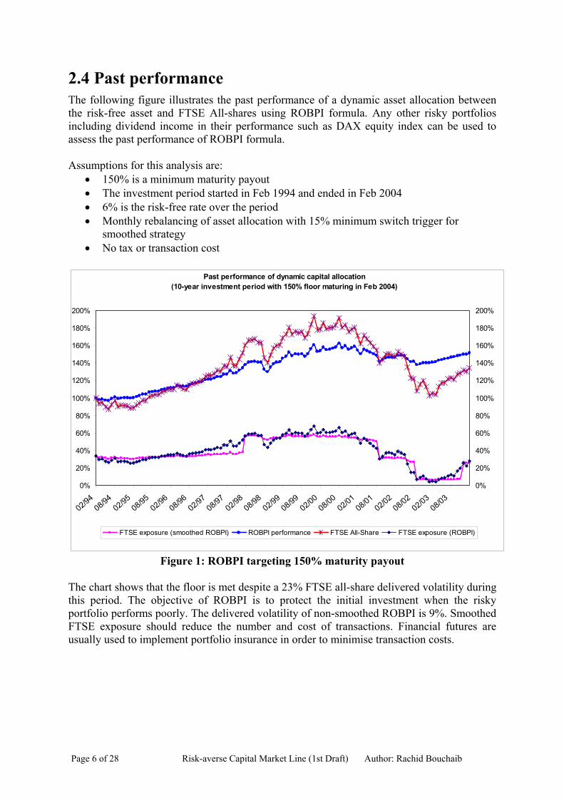
The following figure shows performance of floating ROBPI versus dynamic ROBPI starting from the same initial asset allocation.
Past performance of dynamic capital allocation using ROBPI(10-year investment with 150% floor maturing in Feb 2004)
0%
20%
40%
60%
80%
100%
120%
140%
160%
180%
200%
02/94
08/94
02/95
08/95
02/96
08/96
02/97
08/97
02/98
08/98
02/99
08/99
02/00
08/00
02/01
08/01
02/02
08/02
02/03
08/03
0%
20%
40%
60%
80%
100%
120%
140%
160%
180%
200%
FTSE exposure (smoothed ROBPI) ROBPI performance Floating ROBPI Performance
FTSE All-Share FTSE exposure (ROBPI)
Figure 2: Floating ROBPI versus Dynamic ROBPI
In this example, dynamic ROBPI gave a lower performance reflecting the implicit cost of having the downside risk under-control with more certainty. Floating ROBPI involves no asset allocation changes benefiting from not having to reverse asset allocation changes, which damages the performance of systematic portfolio insurance. Floating ROBPI outperforms dynamic ROBPI in the middle percentiles of risky asset performance while dynamic ROBPI produces higher returns in other more extreme scenarios. The downside-risk with a floating strategy is higher than dynamic strategy reflecting lower performance in the lower percentiles. Such scenarios materialise with continuous risky asset price falls.
Page 7 of 28 Risk-averse Capital Market Line (1st Draft) Author: Rachid Bouchaib
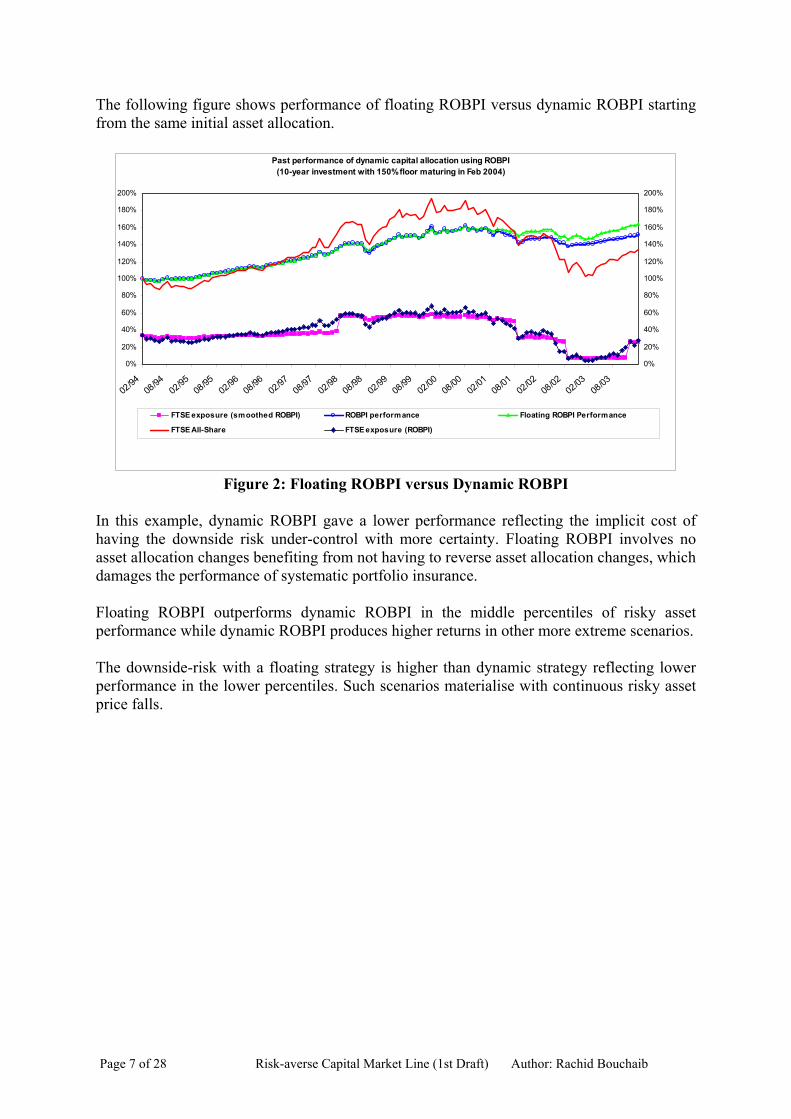
The following figure shows another example of ROBPI performance based on the FTSE All-Share index targeting a 100% floor over a 6-year period starting in Feb 2001
Initial performance of dynamic capital allocation using ROBPI(5-year investment with 100% floor maturing in 2006)
0%
20%
40%
60%
80%
100%
120%
02/0104/01
06/0108/01
10/0112/01
02/0204/02
06/0208/02
10/0212/02
02/0304/03
06/0308/03
10/03
0%
20%
40%
60%
80%
100%
120%
FTSE exposure (smoothed ROBPI) ROBPI performance FTSE All-Share FTSE exposure (ROBPI)
Figure 3: ROBPI targeting 100% floor over 5-year period maturing in Feb 2007
FTSE All-shares delivered volatility over this period is 21%. Over the same time, ROBPI formula produced a portfolio with a 6% delivered volatility. The figure shows that exposure to FTSE All-share was reduced by 30% due to extreme market falls during this period representing the worst equity performance for decades. Nevertheless, the performance of ROBPI shows that the downside-risk is under control. ROBPI performance depends on the accuracy of predicting risky asset volatility, which should improve ROBPI performance.
Page 8 of 28 Risk-averse Capital Market Line (1st Draft) Author: Rachid Bouchaib
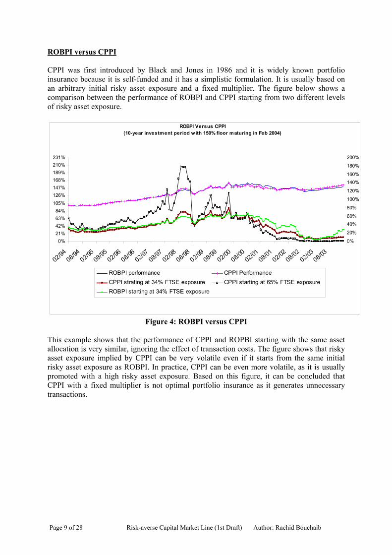
ROBPI versus CPPI CPPI was first introduced by Black and Jones in 1986 and it is widely known portfolio insurance because it is self-funded and it has a simplistic formulation. It is usually based on an arbitrary initial risky asset exposure and a fixed multiplier. The figure below shows a comparison between the performance of ROBPI and CPPI starting from two different levels of risky asset exposure.
ROBPI Versus CPPI(10-year investment period with 150% floor maturing in Feb 2004)
0%21%42%63%84%
105%126%147%168%189%210%231%
02/9408/94
02/9508/95
02/9608/96
02/9708/97
02/9808/98
02/9908/99
02/0008/00
02/0108/01
02/0208/02
02/0308/03
0%
20%
40%60%
80%
100%
120%
140%160%
180%
200%
ROBPI performance CPPI PerformanceCPPI strating at 34% FTSE exposure CPPI starting at 65% FTSE exposureROBPI starting at 34% FTSE exposure
Figure 4: ROBPI versus CPPI
This example shows that the performance of CPPI and ROPBI starting with the same asset allocation is very similar, ignoring the effect of transaction costs. The figure shows that risky asset exposure implied by CPPI can be very volatile even if it starts from the same initial risky asset exposure as ROBPI. In practice, CPPI can be even more volatile, as it is usually promoted with a high risky asset exposure. Based on this figure, it can be concluded that CPPI with a fixed multiplier is not optimal portfolio insurance as it generates unnecessary transactions.
Page 9 of 28 Risk-averse Capital Market Line (1st Draft) Author: Rachid Bouchaib
3 Application to life insurance and pension funds 3.1 Investment strategy for Participating funds Participating funds are typical self-funded portfolios providing smoothed equity exposure with certain levels of guarantees and maturity benefits. Maintaining a balance between meeting guarantees and offering a high level of equity exposure to maximise expected return using a single asset allocation has been a major challenge for life offices. In the past, life offices in the UK focused on adopting a high equity exposure to attract new investors assuming that smoothing payouts to policyholders is sufficient to sustain asset volatility. High equity volatility combined with high equity exposure defeated the resilience of this idea, as assets can be more volatile than liabilities. Linking equity exposure to assets and liabilities provides a downside-risk framework to balance ruin probability minimisation and expected returns maximisation. ROBPI provides a framework to manage life funds with minimum maturity payouts minimising external funding requirement. Liability modelling This section discusses how ROBPI can be used as an investment strategy for asset shares in participating funds in a UK context. As seen in previous sections, deciding the level of downside-risk protection is the main parameter in the asset allocation decision. Applying ROBPI to asset shares implies that an appropriate liability measure needs to be identified as a measure of the present value of the floor. Bonus Reserve Valuation (BRV) is a suitable liability measure for this purpose as it includes the following:
• Future bonuses • Tax on shareholder transfers, charges and investment expenses • Future contractual premiums • Intrinsic value of No-MVR guarantees • Intrinsic value of Guarantees (minimum bonuses, GMP, ROME) • Intrinsic value of Glidepath and smoothing costs.
GAO cost should be excluded from the liability backed by asset shares. It is linked to the total payout; maximising returns on asset shares increase costs of these options. Such option should be managed and hedged within the Estate. Applying ROBPI to participating s gives the following asset allocation
( ) ( )( ) ( )21
21
/ dNdNBRV
SAdNdNWf
−⋅
⋅−=
Where ( )
T
TBRV
SALnd
σ
σ ⋅+
=2/ 2
1 and Tdd σ−= 12
SA / represents asset shares or a higher amount backing the investment strategy.
Page 10 of 28 Risk-averse Capital Market Line (1st Draft) Author: Rachid Bouchaib
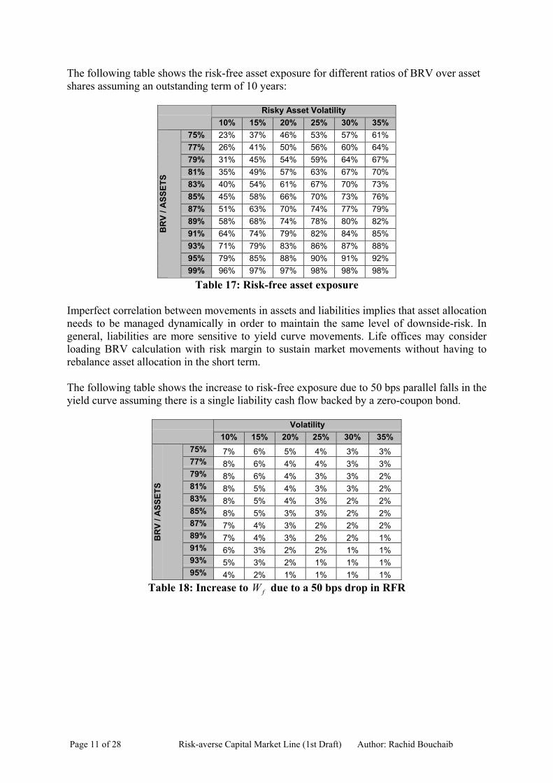
The following table shows the risk-free asset exposure for different ratios of BRV over asset shares assuming an outstanding term of 10 years:
Risky Asset Volatility 10% 15% 20% 25% 30% 35%
75% 23% 37% 46% 53% 57% 61% 77% 26% 41% 50% 56% 60% 64% 79% 31% 45% 54% 59% 64% 67% 81% 35% 49% 57% 63% 67% 70% 83% 40% 54% 61% 67% 70% 73% 85% 45% 58% 66% 70% 73% 76% 87% 51% 63% 70% 74% 77% 79% 89% 58% 68% 74% 78% 80% 82% 91% 64% 74% 79% 82% 84% 85% 93% 71% 79% 83% 86% 87% 88% 95% 79% 85% 88% 90% 91% 92%
BR
V / A
SSET
S
99% 96% 97% 97% 98% 98% 98%
Table 17: Risk-free asset exposure Imperfect correlation between movements in assets and liabilities implies that asset allocation needs to be managed dynamically in order to maintain the same level of downside-risk. In general, liabilities are more sensitive to yield curve movements. Life offices may consider loading BRV calculation with risk margin to sustain market movements without having to rebalance asset allocation in the short term. The following table shows the increase to risk-free exposure due to 50 bps parallel falls in the yield curve assuming there is a single liability cash flow backed by a zero-coupon bond.
Volatility 10% 15% 20% 25% 30% 35%
75% 7% 6% 5% 4% 3% 3% 77% 8% 6% 4% 4% 3% 3% 79% 8% 6% 4% 3% 3% 2% 81% 8% 5% 4% 3% 3% 2% 83% 8% 5% 4% 3% 2% 2% 85% 8% 5% 3% 3% 2% 2% 87% 7% 4% 3% 2% 2% 2% 89% 7% 4% 3% 2% 2% 1% 91% 6% 3% 2% 2% 1% 1% 93% 5% 3% 2% 1% 1% 1%
BR
V / A
SSET
S
95% 4% 2% 1% 1% 1% 1% Table 18: Increase to W due to a 50 bps drop in RFR f
Page 11 of 28 Risk-averse Capital Market Line (1st Draft) Author: Rachid Bouchaib
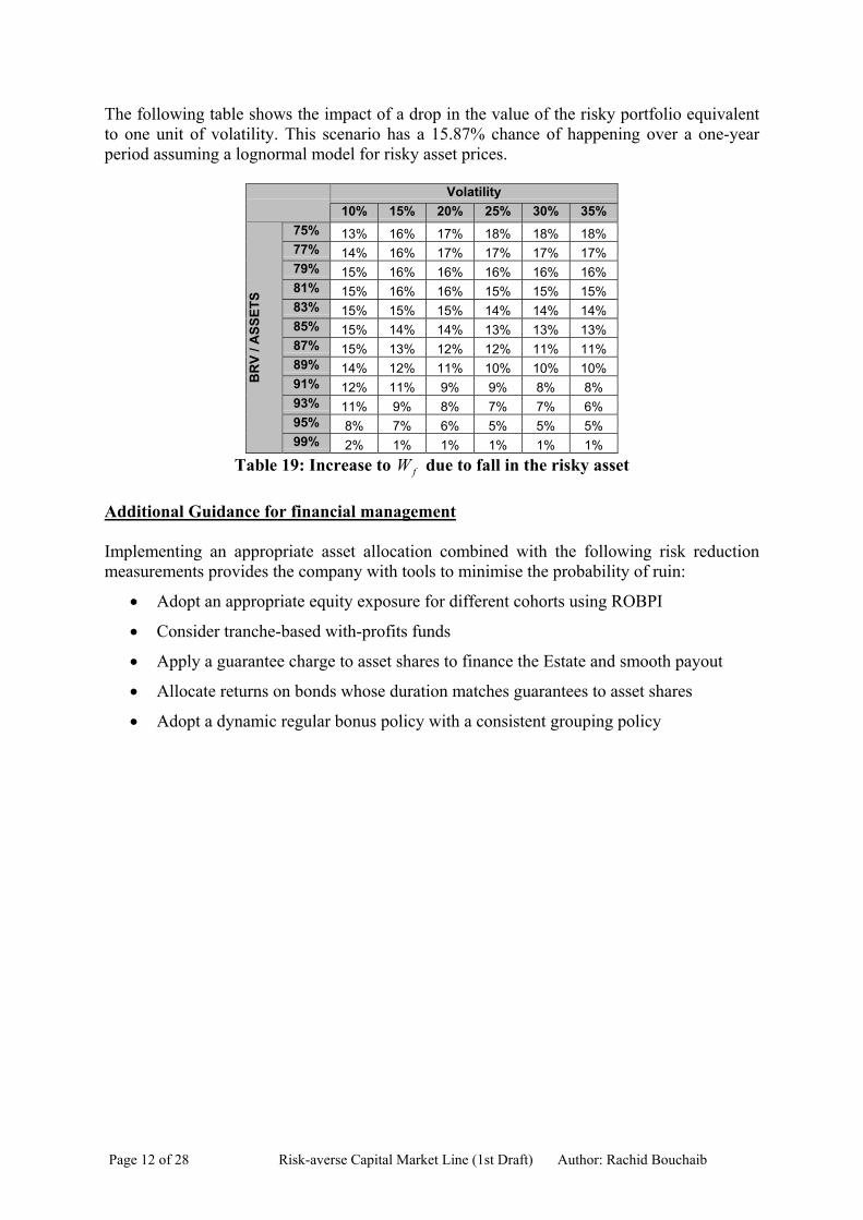
The following table shows the impact of a drop in the value of the risky portfolio equivalent to one unit of volatility. This scenario has a 15.87% chance of happening over a one-year period assuming a lognormal model for risky asset prices.
Volatility 10% 15% 20% 25% 30% 35%
75% 13% 16% 17% 18% 18% 18% 77% 14% 16% 17% 17% 17% 17% 79% 15% 16% 16% 16% 16% 16% 81% 15% 16% 16% 15% 15% 15% 83% 15% 15% 15% 14% 14% 14% 85% 15% 14% 14% 13% 13% 13% 87% 15% 13% 12% 12% 11% 11% 89% 14% 12% 11% 10% 10% 10% 91% 12% 11% 9% 9% 8% 8% 93% 11% 9% 8% 7% 7% 6% 95% 8% 7% 6% 5% 5% 5%
BR
V / A
SSET
S
99% 2% 1% 1% 1% 1% 1% Table 19: Increase to W due to fall in the risky asset f
Additional Guidance for financial management Implementing an appropriate asset allocation combined with the following risk reduction measurements provides the company with tools to minimise the probability of ruin:
• Adopt an appropriate equity exposure for different cohorts using ROBPI
• Consider tranche-based with-profits funds
• Apply a guarantee charge to asset shares to finance the Estate and smooth payout
• Allocate returns on bonds whose duration matches guarantees to asset shares
• Adopt a dynamic regular bonus policy with a consistent grouping policy
Page 12 of 28 Risk-averse Capital Market Line (1st Draft) Author: Rachid Bouchaib
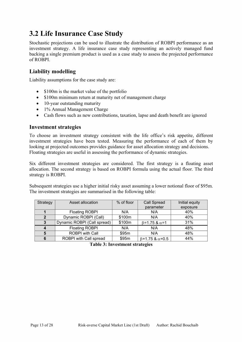
3.2 Life Insurance Case Study Stochastic projections can be used to illustrate the distribution of ROBPI performance as an investment strategy. A life insurance case study representing an actively managed fund backing a single premium product is used as a case study to assess the projected performance of ROBPI.
Liability modelling Liability assumptions for the case study are:
• $100m is the market value of the portfolio • $100m minimum return at maturity net of management charge • 10-year outstanding maturity • 1% Annual Management Charge • Cash flows such as new contributions, taxation, lapse and death benefit are ignored
Investment strategies To choose an investment strategy consistent with the life office’s risk appetite, different investment strategies have been tested. Measuring the performance of each of them by looking at projected outcomes provides guidance for asset allocation strategy and decisions. Floating strategies are useful in assessing the performance of dynamic strategies. Six different investment strategies are considered. The first strategy is a floating asset allocation. The second strategy is based on ROBPI formula using the actual floor. The third strategy is ROBPI. Subsequent strategies use a higher initial risky asset assuming a lower notional floor of $95m. The investment strategies are summarised in the following table:
Strategy Asset allocation % of floor Call Spread parameter
Initial equity exposure
1 Floating ROBPI N/A N/A 40% 2 Dynamic ROBPI (Call) $100m N/A 40% 3 Dynamic ROBPI (Call spread) $100m β=1.75 & α=1 31% 4 Floating ROBPI N/A N/A 48% 5 ROBPI with Call $95m N/A 48% 6 ROBPI with Call spread $95m β=1.75 & α=0.5 44%
Table 3: Investment strategies
Page 13 of 28 Risk-averse Capital Market Line (1st Draft) Author: Rachid Bouchaib
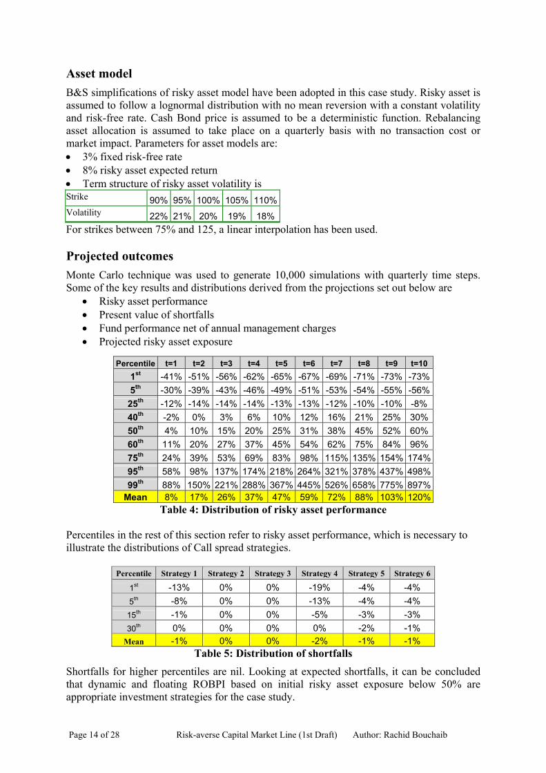
Asset model B&S simplifications of risky asset model have been adopted in this case study. Risky asset is assumed to follow a lognormal distribution with no mean reversion with a constant volatility and risk-free rate. Cash Bond price is assumed to be a deterministic function. Rebalancing asset allocation is assumed to take place on a quarterly basis with no transaction cost or market impact. Parameters for asset models are: • 3% fixed risk-free rate • 8% risky asset expected return • Term structure of risky asset volatility is Strike 90% 95% 100% 105% 110%Volatility 22% 21% 20% 19% 18%For strikes between 75% and 125, a linear interpolation has been used. Projected outcomes Monte Carlo technique was used to generate 10,000 simulations with quarterly time steps. Some of the key results and distributions derived from the projections set out below are
• Risky asset performance • Present value of shortfalls • Fund performance net of annual management charges • Projected risky asset exposure
Percentile t=1 t=2 t=3 t=4 t=5 t=6 t=7 t=8 t=9 t=10
1st -41% -51% -56% -62% -65% -67% -69% -71% -73% -73% 5th -30% -39% -43% -46% -49% -51% -53% -54% -55% -56% 25th -12% -14% -14% -14% -13% -13% -12% -10% -10% -8% 40th -2% 0% 3% 6% 10% 12% 16% 21% 25% 30% 50th 4% 10% 15% 20% 25% 31% 38% 45% 52% 60% 60th 11% 20% 27% 37% 45% 54% 62% 75% 84% 96% 75th 24% 39% 53% 69% 83% 98% 115% 135% 154% 174% 95th 58% 98% 137% 174% 218% 264% 321% 378% 437% 498% 99th 88% 150% 221% 288% 367% 445% 526% 658% 775% 897%
Mean 8% 17% 26% 37% 47% 59% 72% 88% 103% 120% Table 4: Distribution of risky asset performance
Percentiles in the rest of this section refer to risky asset performance, which is necessary to illustrate the distributions of Call spread strategies.
Percentile Strategy 1 Strategy 2 Strategy 3 Strategy 4 Strategy 5 Strategy 6
1st -13% 0% 0% -19% -4% -4% 5th -8% 0% 0% -13% -4% -4%
15th -1% 0% 0% -5% -3% -3% 30th 0% 0% 0% 0% -2% -1%
Mean -1% 0% 0% -2% -1% -1% Table 5: Distribution of shortfalls
Shortfalls for higher percentiles are nil. Looking at expected shortfalls, it can be concluded that dynamic and floating ROBPI based on initial risky asset exposure below 50% are appropriate investment strategies for the case study.
Page 14 of 28 Risk-averse Capital Market Line (1st Draft) Author: Rachid Bouchaib
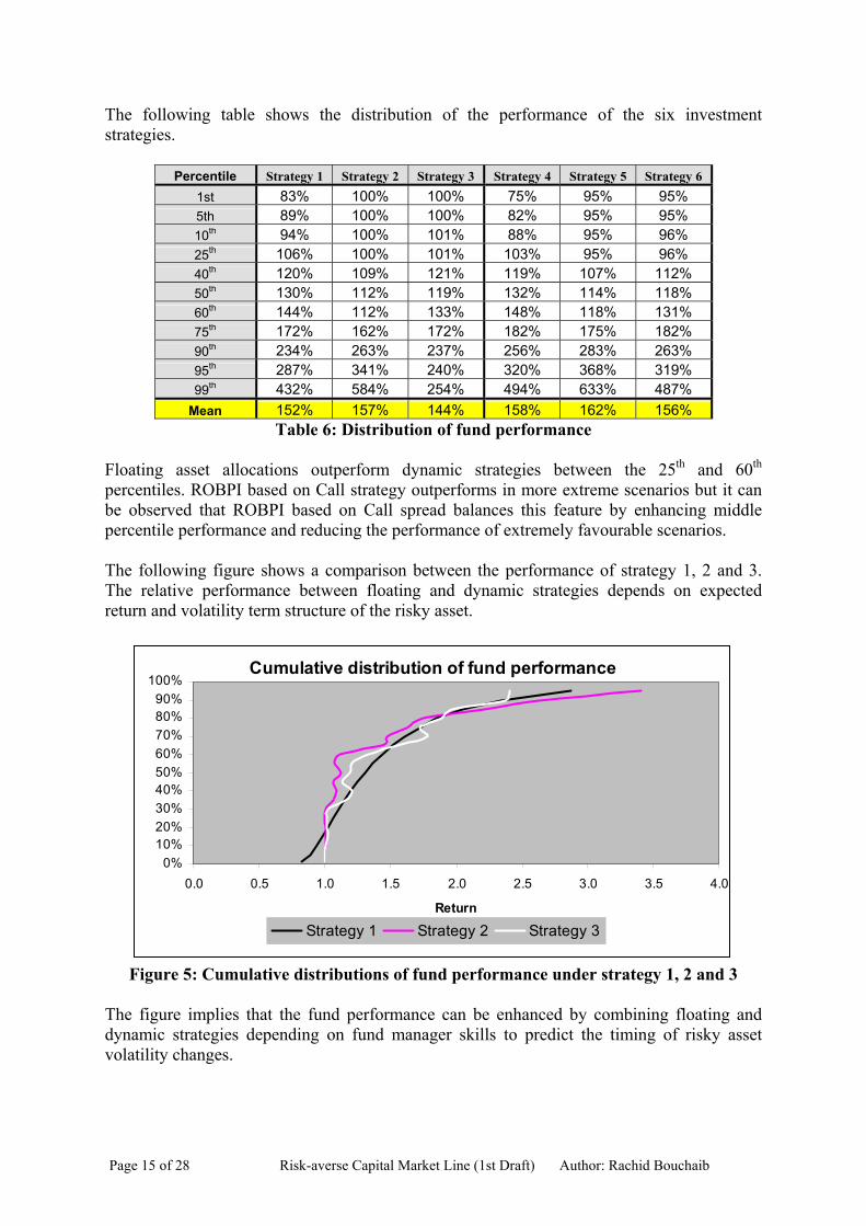
The following table shows the distribution of the performance of the six investment strategies.
Percentile Strategy 1 Strategy 2 Strategy 3 Strategy 4 Strategy 5 Strategy 6 1st 83% 100% 100% 75% 95% 95% 5th 89% 100% 100% 82% 95% 95% 10th 94% 100% 101% 88% 95% 96% 25th 106% 100% 101% 103% 95% 96% 40th 120% 109% 121% 119% 107% 112% 50th 130% 112% 119% 132% 114% 118% 60th 144% 112% 133% 148% 118% 131% 75th 172% 162% 172% 182% 175% 182% 90th 234% 263% 237% 256% 283% 263% 95th 287% 341% 240% 320% 368% 319% 99th 432% 584% 254% 494% 633% 487%
Mean 152% 157% 144% 158% 162% 156% Table 6: Distribution of fund performance
Floating asset allocations outperform dynamic strategies between the 25th and 60th percentiles. ROBPI based on Call strategy outperforms in more extreme scenarios but it can be observed that ROBPI based on Call spread balances this feature by enhancing middle percentile performance and reducing the performance of extremely favourable scenarios. The following figure shows a comparison between the performance of strategy 1, 2 and 3. The relative performance between floating and dynamic strategies depends on expected return and volatility term structure of the risky asset.
Cumulative distribution of fund performance
0%10%20%30%40%50%60%70%80%90%
100%
0.0 0.5 1.0 1.5 2.0 2.5 3.0 3.5 4
Return
.0
Strategy 1 Strategy 2 Strategy 3
Figure 5: Cumulative distributions of fund performance under strategy 1, 2 and 3
The figure implies that the fund performance can be enhanced by combining floating and dynamic strategies depending on fund manager skills to predict the timing of risky asset volatility changes.
Page 15 of 28 Risk-averse Capital Market Line (1st Draft) Author: Rachid Bouchaib
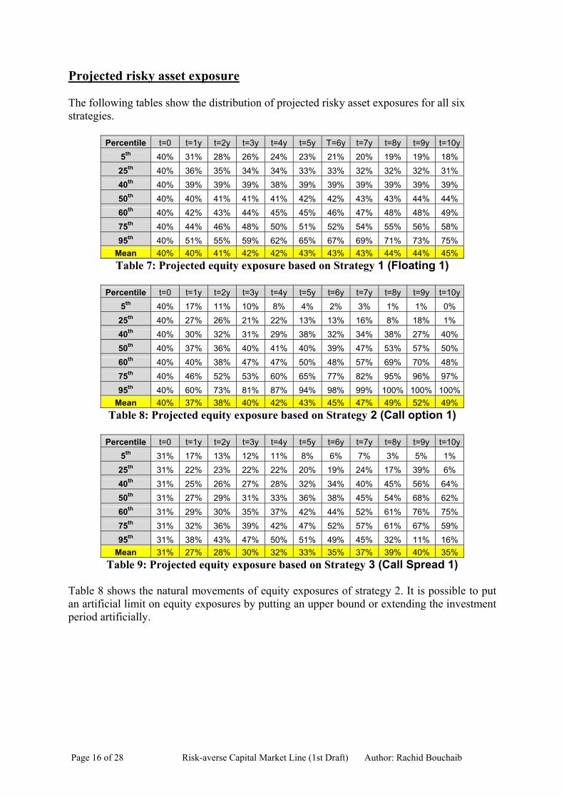
Projected risky asset exposure The following tables show the distribution of projected risky asset exposures for all six strategies.
Percentile t=0 t=1y t=2y t=3y t=4y t=5y T=6y t=7y t=8y t=9y t=10y 5th 40% 31% 28% 26% 24% 23% 21% 20% 19% 19% 18%
25th 40% 36% 35% 34% 34% 33% 33% 32% 32% 32% 31% 40th 40% 39% 39% 39% 38% 39% 39% 39% 39% 39% 39% 50th 40% 40% 41% 41% 41% 42% 42% 43% 43% 44% 44% 60th 40% 42% 43% 44% 45% 45% 46% 47% 48% 48% 49% 75th 40% 44% 46% 48% 50% 51% 52% 54% 55% 56% 58% 95th 40% 51% 55% 59% 62% 65% 67% 69% 71% 73% 75%
Mean 40% 40% 41% 42% 42% 43% 43% 43% 44% 44% 45% Table 7: Projected equity exposure based on Strategy 1 (Floating 1)
Percentile t=0 t=1y t=2y t=3y t=4y t=5y t=6y t=7y t=8y t=9y t=10y
5th 40% 17% 11% 10% 8% 4% 2% 3% 1% 1% 0% 25th 40% 27% 26% 21% 22% 13% 13% 16% 8% 18% 1% 40th 40% 30% 32% 31% 29% 38% 32% 34% 38% 27% 40% 50th 40% 37% 36% 40% 41% 40% 39% 47% 53% 57% 50% 60th 40% 40% 38% 47% 47% 50% 48% 57% 69% 70% 48% 75th 40% 46% 52% 53% 60% 65% 77% 82% 95% 96% 97% 95th 40% 60% 73% 81% 87% 94% 98% 99% 100% 100% 100%
Mean 40% 37% 38% 40% 42% 43% 45% 47% 49% 52% 49% Table 8: Projected equity exposure based on Strategy 2 (Call option 1)
Percentile t=0 t=1y t=2y t=3y t=4y t=5y t=6y t=7y t=8y t=9y t=10y
5th 31% 17% 13% 12% 11% 8% 6% 7% 3% 5% 1% 25th 31% 22% 23% 22% 22% 20% 19% 24% 17% 39% 6% 40th 31% 25% 26% 27% 28% 32% 34% 40% 45% 56% 64% 50th 31% 27% 29% 31% 33% 36% 38% 45% 54% 68% 62% 60th 31% 29% 30% 35% 37% 42% 44% 52% 61% 76% 75% 75th 31% 32% 36% 39% 42% 47% 52% 57% 61% 67% 59% 95th 31% 38% 43% 47% 50% 51% 49% 45% 32% 11% 16%
Mean 31% 27% 28% 30% 32% 33% 35% 37% 39% 40% 35% Table 9: Projected equity exposure based on Strategy 3 (Call Spread 1)
Table 8 shows the natural movements of equity exposures of strategy 2. It is possible to put an artificial limit on equity exposures by putting an upper bound or extending the investment period artificially.
Page 16 of 28 Risk-averse Capital Market Line (1st Draft) Author: Rachid Bouchaib
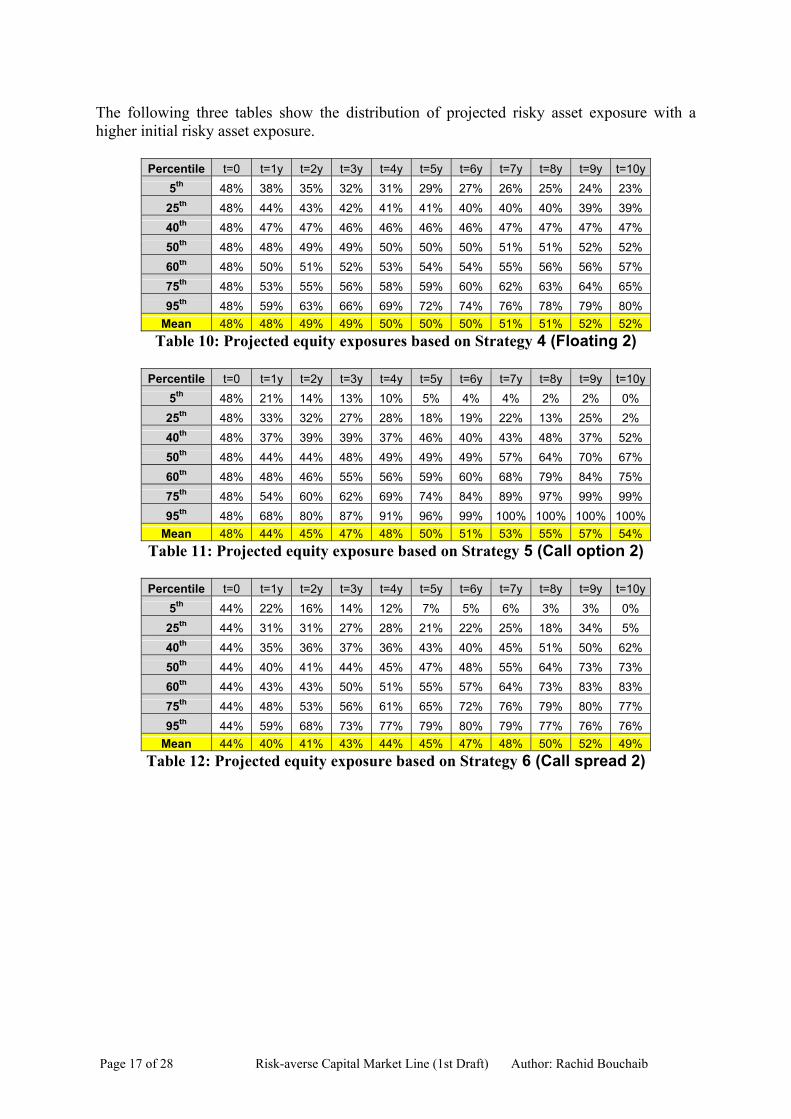
The following three tables show the distribution of projected risky asset exposure with a higher initial risky asset exposure.
Percentile t=0 t=1y t=2y t=3y t=4y t=5y t=6y t=7y t=8y t=9y t=10y 5th 48% 38% 35% 32% 31% 29% 27% 26% 25% 24% 23%
25th 48% 44% 43% 42% 41% 41% 40% 40% 40% 39% 39% 40th 48% 47% 47% 46% 46% 46% 46% 47% 47% 47% 47% 50th 48% 48% 49% 49% 50% 50% 50% 51% 51% 52% 52% 60th 48% 50% 51% 52% 53% 54% 54% 55% 56% 56% 57% 75th 48% 53% 55% 56% 58% 59% 60% 62% 63% 64% 65% 95th 48% 59% 63% 66% 69% 72% 74% 76% 78% 79% 80%
Mean 48% 48% 49% 49% 50% 50% 50% 51% 51% 52% 52% Table 10: Projected equity exposures based on Strategy 4 (Floating 2)
Percentile t=0 t=1y t=2y t=3y t=4y t=5y t=6y t=7y t=8y t=9y t=10y
5th 48% 21% 14% 13% 10% 5% 4% 4% 2% 2% 0% 25th 48% 33% 32% 27% 28% 18% 19% 22% 13% 25% 2% 40th 48% 37% 39% 39% 37% 46% 40% 43% 48% 37% 52% 50th 48% 44% 44% 48% 49% 49% 49% 57% 64% 70% 67% 60th 48% 48% 46% 55% 56% 59% 60% 68% 79% 84% 75% 75th 48% 54% 60% 62% 69% 74% 84% 89% 97% 99% 99% 95th 48% 68% 80% 87% 91% 96% 99% 100% 100% 100% 100%
Mean 48% 44% 45% 47% 48% 50% 51% 53% 55% 57% 54% Table 11: Projected equity exposure based on Strategy 5 (Call option 2)
Percentile t=0 t=1y t=2y t=3y t=4y t=5y t=6y t=7y t=8y t=9y t=10y
5th 44% 22% 16% 14% 12% 7% 5% 6% 3% 3% 0% 25th 44% 31% 31% 27% 28% 21% 22% 25% 18% 34% 5% 40th 44% 35% 36% 37% 36% 43% 40% 45% 51% 50% 62% 50th 44% 40% 41% 44% 45% 47% 48% 55% 64% 73% 73% 60th 44% 43% 43% 50% 51% 55% 57% 64% 73% 83% 83% 75th 44% 48% 53% 56% 61% 65% 72% 76% 79% 80% 77% 95th 44% 59% 68% 73% 77% 79% 80% 79% 77% 76% 76%
Mean 44% 40% 41% 43% 44% 45% 47% 48% 50% 52% 49% Table 12: Projected equity exposure based on Strategy 6 (Call spread 2)
Page 17 of 28 Risk-averse Capital Market Line (1st Draft) Author: Rachid Bouchaib

The following two figures show the distribution of risky asset exposure for floating strategy 1 and dynamic strategy 2. They show that dynamic asset allocation gives a wider range of risky asset exposure.
Distribution of risky asset exposure for Strategy 1
0%
10%
20%
30%
40%
50%
60%
70%
80%
90%
0 1 2 3 4 5 6 7 8 9 10
Risk
y as
set e
xpos
ure
Figure 6: Risky asset exposure distribution for strategy 1
Distribution of risky asset exposure for Strategy 2
0%
10%
20%
30%
40%
50%
60%
70%
80%
90%
100%
0 1 2 3 4 5 6 7 8 9 10
Ris
ky a
sset
exp
osur
e
Figure 7: Risky asset exposure distribution for strategy 2
Page 18 of 28 Risk-averse Capital Market Line (1st Draft) Author: Rachid Bouchaib
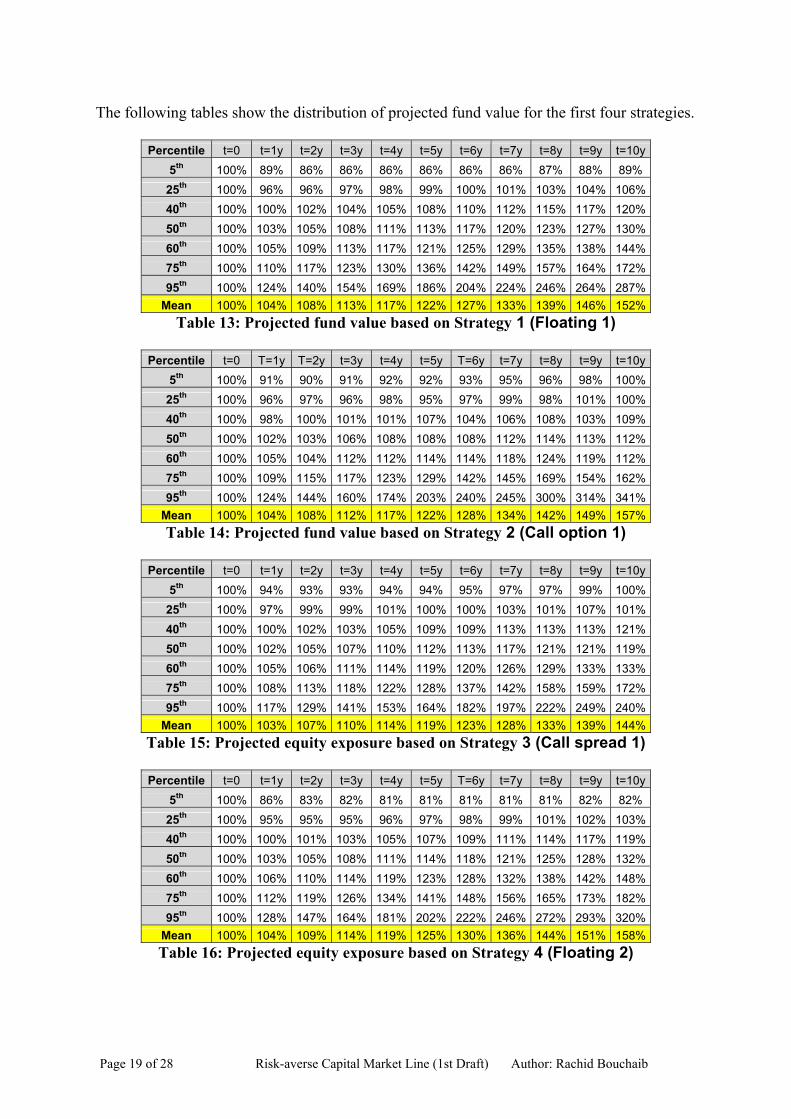
The following tables show the distribution of projected fund value for the first four strategies.
Percentile t=0 t=1y t=2y t=3y t=4y t=5y t=6y t=7y t=8y t=9y t=10y 5th 100% 89% 86% 86% 86% 86% 86% 86% 87% 88% 89%
25th 100% 96% 96% 97% 98% 99% 100% 101% 103% 104% 106% 40th 100% 100% 102% 104% 105% 108% 110% 112% 115% 117% 120% 50th 100% 103% 105% 108% 111% 113% 117% 120% 123% 127% 130% 60th 100% 105% 109% 113% 117% 121% 125% 129% 135% 138% 144% 75th 100% 110% 117% 123% 130% 136% 142% 149% 157% 164% 172% 95th 100% 124% 140% 154% 169% 186% 204% 224% 246% 264% 287%
Mean 100% 104% 108% 113% 117% 122% 127% 133% 139% 146% 152% Table 13: Projected fund value based on Strategy 1 (Floating 1)
Percentile t=0 T=1y T=2y t=3y t=4y t=5y T=6y t=7y t=8y t=9y t=10y
5th 100% 91% 90% 91% 92% 92% 93% 95% 96% 98% 100% 25th 100% 96% 97% 96% 98% 95% 97% 99% 98% 101% 100% 40th 100% 98% 100% 101% 101% 107% 104% 106% 108% 103% 109% 50th 100% 102% 103% 106% 108% 108% 108% 112% 114% 113% 112% 60th 100% 105% 104% 112% 112% 114% 114% 118% 124% 119% 112% 75th 100% 109% 115% 117% 123% 129% 142% 145% 169% 154% 162% 95th 100% 124% 144% 160% 174% 203% 240% 245% 300% 314% 341%
Mean 100% 104% 108% 112% 117% 122% 128% 134% 142% 149% 157% Table 14: Projected fund value based on Strategy 2 (Call option 1)
Percentile t=0 t=1y t=2y t=3y t=4y t=5y t=6y t=7y t=8y t=9y t=10y
5th 100% 94% 93% 93% 94% 94% 95% 97% 97% 99% 100% 25th 100% 97% 99% 99% 101% 100% 100% 103% 101% 107% 101% 40th 100% 100% 102% 103% 105% 109% 109% 113% 113% 113% 121% 50th 100% 102% 105% 107% 110% 112% 113% 117% 121% 121% 119% 60th 100% 105% 106% 111% 114% 119% 120% 126% 129% 133% 133% 75th 100% 108% 113% 118% 122% 128% 137% 142% 158% 159% 172% 95th 100% 117% 129% 141% 153% 164% 182% 197% 222% 249% 240%
Mean 100% 103% 107% 110% 114% 119% 123% 128% 133% 139% 144% Table 15: Projected equity exposure based on Strategy 3 (Call spread 1)
Percentile t=0 t=1y t=2y t=3y t=4y t=5y T=6y t=7y t=8y t=9y t=10y
5th 100% 86% 83% 82% 81% 81% 81% 81% 81% 82% 82% 25th 100% 95% 95% 95% 96% 97% 98% 99% 101% 102% 103% 40th 100% 100% 101% 103% 105% 107% 109% 111% 114% 117% 119% 50th 100% 103% 105% 108% 111% 114% 118% 121% 125% 128% 132% 60th 100% 106% 110% 114% 119% 123% 128% 132% 138% 142% 148% 75th 100% 112% 119% 126% 134% 141% 148% 156% 165% 173% 182% 95th 100% 128% 147% 164% 181% 202% 222% 246% 272% 293% 320%
Mean 100% 104% 109% 114% 119% 125% 130% 136% 144% 151% 158% Table 16: Projected equity exposure based on Strategy 4 (Floating 2)
Page 19 of 28 Risk-averse Capital Market Line (1st Draft) Author: Rachid Bouchaib
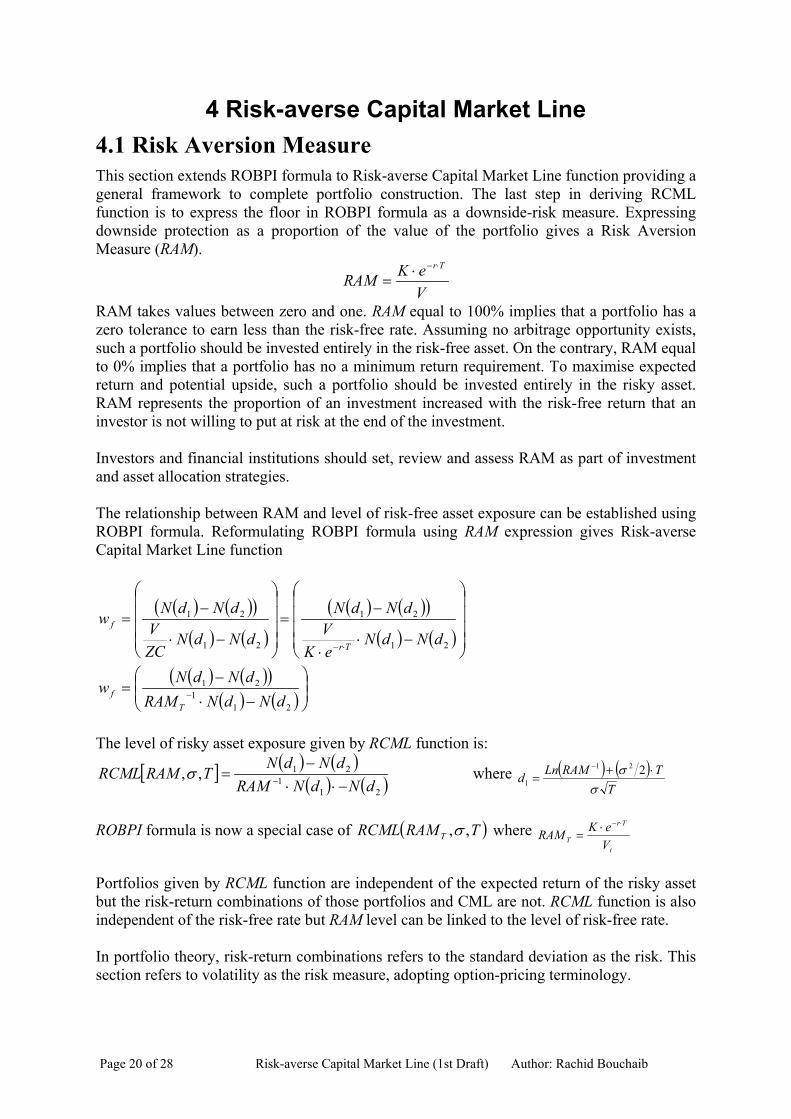
4 Risk-averse Capital Market Line 4.1 Risk Aversion Measure This section extends ROBPI formula to Risk-averse Capital Market Line function providing a general framework to complete portfolio construction. The last step in deriving RCML function is to express the floor in ROBPI formula as a downside-risk measure. Expressing downside protection as a proportion of the value of the portfolio gives a Risk Aversion Measure (RAM).
VeKRAM
Tr⋅−⋅=
RAM takes values between zero and one. RAM equal to 100% implies that a portfolio has a zero tolerance to earn less than the risk-free rate. Assuming no arbitrage opportunity exists, such a portfolio should be invested entirely in the risk-free asset. On the contrary, RAM equal to 0% implies that a portfolio has no a minimum return requirement. To maximise expected return and potential upside, such a portfolio should be invested entirely in the risky asset. RAM represents the proportion of an investment increased with the risk-free return that an investor is not willing to put at risk at the end of the investment. Investors and financial institutions should set, review and assess RAM as part of investment and asset allocation strategies. The relationship between RAM and level of risk-free asset exposure can be established using ROBPI formula. Reformulating ROBPI formula using RAM expression gives Risk-averse Capital Market Line function
( ) ( )( )( ) ( )
( ) ( )( )( ) ( )
−⋅⋅
−=
−⋅
−=
⋅− 21
21
21
21
dNdNeKV
dNdN
dNdNZCV
dNdNw
Tr
f
( ) ( )( )( ) ( )
−⋅−
= −21
121
dNdNRAMdNdN
wT
f
The level of risky asset exposure given by RCML function is:
[ ] ( ) ( )( ) ( )21
121,,
dNdNRAMdNdNTRAMRCML−⋅⋅
−= −σ where ( ) ( )
TTRAMLnd
σσ ⋅+
=− 221
1
ROBPI formula is now a special case of ( )TRAMRCML T ,,σ where
t
Tr
T VeKRAM
⋅−⋅=
Portfolios given by RCML function are independent of the expected return of the risky asset but the risk-return combinations of those portfolios and CML are not. RCML function is also independent of the risk-free rate but RAM level can be linked to the level of risk-free rate. In portfolio theory, risk-return combinations refers to the standard deviation as the risk. This section refers to volatility as the risk measure, adopting option-pricing terminology.
Page 20 of 28 Risk-averse Capital Market Line (1st Draft) Author: Rachid Bouchaib
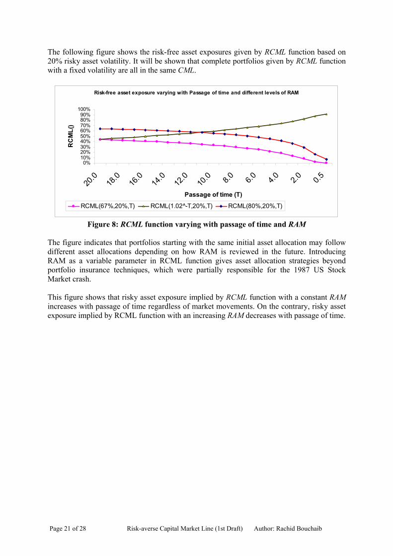
The following figure shows the risk-free asset exposures given by RCML function based on 20% risky asset volatility. It will be shown that complete portfolios given by RCML function with a fixed volatility are all in the same CML.
Risk-free asset exposure varying with Passage of time and different levels of RAM
0%10%20%30%40%50%60%70%80%90%
100%
20.0
18.0
16.0
14.0
12.0
10.0 8.0 6.0 4.0 2.0 0.5
Passage of time (T)
RC
ML(
)
RCML(67%,20%,T) RCML(1.02^-T,20%,T) RCML(80%,20%,T)
Figure 8: RCML function varying with passage of time and RAM
The figure indicates that portfolios starting with the same initial asset allocation may follow different asset allocations depending on how RAM is reviewed in the future. Introducing RAM as a variable parameter in RCML function gives asset allocation strategies beyond portfolio insurance techniques, which were partially responsible for the 1987 US Stock Market crash. This figure shows that risky asset exposure implied by RCML function with a constant RAM increases with passage of time regardless of market movements. On the contrary, risky asset exposure implied by RCML function with an increasing RAM decreases with passage of time.
Page 21 of 28 Risk-averse Capital Market Line (1st Draft) Author: Rachid Bouchaib
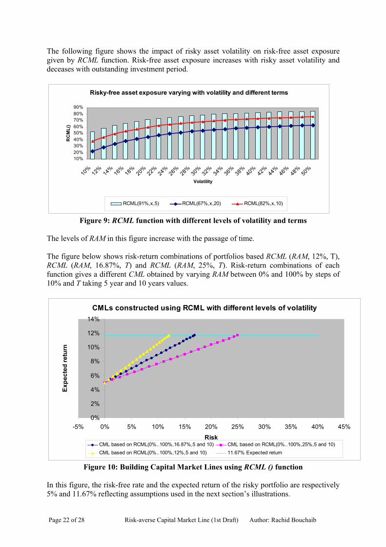
The following figure shows the impact of risky asset volatility on risk-free asset exposure given by RCML function. Risk-free asset exposure increases with risky asset volatility and deceases with outstanding investment period.
Risky-free asset exposure varying with volatility and different terms
10%20%30%40%50%60%70%80%90%
10%
12%
14%
16%
18%
20%
22%
24%
26%
28%
30%
32%
34%
36%
38%
40%
42%
44%
46%
48%
50%
Volatility
RC
ML(
)
RCML(91%,x,5) RCML(67%,x,20) RCML(82%,x,10)
Figure 9: RCML function with different levels of volatility and terms
The levels of RAM in this figure increase with the passage of time. The figure below shows risk-return combinations of portfolios based RCML (RAM, 12%, T), RCML (RAM, 16.87%, T) and RCML (RAM, 25%, T). Risk-return combinations of each function gives a different CML obtained by varying RAM between 0% and 100% by steps of 10% and T taking 5 year and 10 years values.
CMLs constructed using RCML with different levels of volatility
0%
2%
4%
6%
8%
10%
12%
14%
-5% 0% 5% 10% 15% 20% 25% 30% 35% 40% 45%
Risk
Expe
cted
retu
rn
CML based on RCML(0%..100%,16.87%,5 and 10) CML based on RCML(0%..100%,25%,5 and 10)CML based on RCML(0%..100%,12%,5 and 10) 11.67% Expected return
Figure 10: Building Capital Market Lines using RCML () function
In this figure, the risk-free rate and the expected return of the risky portfolio are respectively 5% and 11.67% reflecting assumptions used in the next section’s illustrations.
Page 22 of 28 Risk-averse Capital Market Line (1st Draft) Author: Rachid Bouchaib
Portfolios with higher RAM are closer to the risk-free asset while lower RAMs give portfolios closer the risky asset. Portfolios at top end of each CML have zero RAM representing portfolios invested entirely in the risky asset. The assumed levels of volatility to generate the three CML are respectively 12%, 16.87% and 25%. Risk-return combinations of portfolios based on RCML function by varying T and RAM give CML for a given volatility of the optimal risky portfolios. The volatility of risky portfolio represents the slope of CML, so varying volatility in RCML function gives different CML. 4.2 Asset allocation with three asset classes This section illustrates how RCML function can be used to guide complete portfolio and CML construction using the risk-free asset and two risky assets. The following assumptions represent a typical example of portfolio theory textbooks Expected return Standard deviation
Equity Index E 15% 50%
Bond Index B 10% 20%
T-bills F 5% 0%
Correlation between E and B is -20%
Markowitz’s optimal risky portfolio W is a portfolio in the efficient frontier with the highest Sharp Ratio. For two risky assets, there is an analytical formula for the optimal risky portfolio, which can be found in most portfolio theory textbooks.
M
The optimal risky portfolio W should be invested as follows M
• 33.33% of W should be invested in the equity index M
• 66.67% of W should be invested in the Bond index M
Or ( %33.33=EW , W ). %67.66=B
The expected return of the optimal risk portfolio is Exp(W ) = 11.67% M
The standard deviation of the optimal portfolio is St(W ) =16.87% M
The Sharpe Ratio (1964) of the optimal portfolio is 39.53% Combining the optimal risky portfolio with risk-free asset exposure given by
function gives a portfolios in CML. It is a straight line starting with the risk-free asset on the left hand-side and ending with the optimal risky portfolio on the right hand-side.
( TRAMRCML %,87.16, )
Every combination of RAM and investment period T gives a unique optimal complete portfolio in CML. Combining all possible risky assets with ( )TRAMRCML %,87.16, gives inefficient frontier with portfolios below CML portfolios. The figure below shows the following risk-return combinations
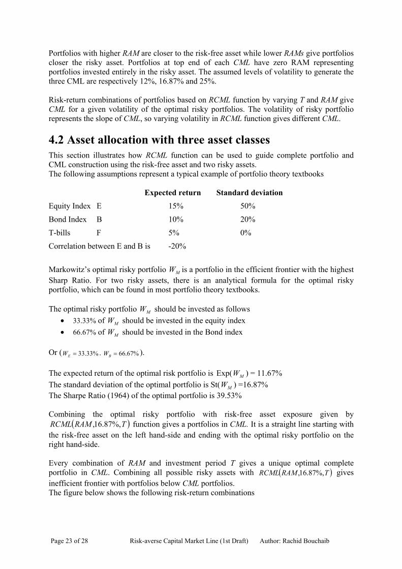
Page 23 of 28 Risk-averse Capital Market Line (1st Draft) Author: Rachid Bouchaib
• Capital Market Line constructed using ( )TRAMRCML %,87.16, function and the efficient risky portfolio
• The efficient frontier of the risky assets (including inefficient portfolios below the minimum variance portfolio)
• All possible combinations of risk-free asset based on ( )10%,87.16%,80RCML and the two risky assets
• All possible combinations of risk-free asset based on ( )5%,87.16%,80RCML and the two risky assets
Risk-averse Capital Market Line
0%
2%
4%
6%
8%
10%
12%
14%
16%
0% 5% 10% 15% 20% 25% 30% 35% 40% 45%
Risk
Expe
cted
Ret
urn
CML based on RCML(x,16.87%,T)
All possible portfolios for RAM=80% {RCML(80%,16.87%,5)=39%}
All possible portfolios for RAM=80% {CML(80%,16.87%,10)=51%}
Markowitz' efficient frontier
Figure 11: Risk-return combinations based on RCML (RAM, 16.87%, T)
The capital market line is the tangent line to the efficient frontier that passes through the risk-free rate on the expected return axis. Portfolios below the minimum variance portfolio ( %14.24=EW and %86.75=BW ) are inefficient. The main conclusion from this figure is that RCML function combined with individual risky assets is not an efficient framework, as it produces portfolios below CML except the optimal risky portfolio. Combining efficient risky portfolio as a single risky asset with the risky-free asset given by RCML function gives complete portfolios and CMLs without any extra optimisation work.
Page 24 of 28 Risk-averse Capital Market Line (1st Draft) Author: Rachid Bouchaib
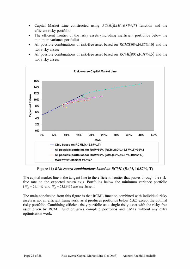
The following figure shows risk-return combinations excluding inefficient portfolios for
• Capital Market Line constructed using ( )TRAMRCML %,87.16, • The efficient frontier of the risky assets • All possible complete portfolios based on ( )5%,87.16%,80RCML • All possible complete portfolios based on ( )5%,87.16%,92RCML
Risk-averse Capital Market Line
0%
2%
4%
6%
8%
10%
12%
14%
16%
0% 5% 10% 15% 20% 25% 30% 35% 40% 45%Risk
Expe
cted
Ret
urn
CML based on RCML(x,16.87%,T)All possible portfolios for RAM=80% {RCML(80%,16.87%,5)=39%}All possible portfolios for RAM=92% {RCML(92%,16.87%,5)=72%}Markowitz' efficient frontier
Figure 12: RCML and Efficient Frontier (Excluding inefficient portfolios)
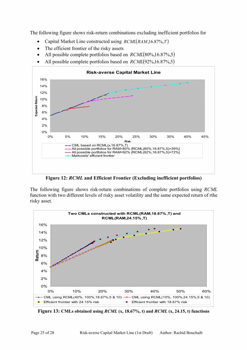
The following figure shows risk-return combinations of complete portfolios using RCML function with two different levels of risky asset volatility and the same expected return of rthe risky asset.
Two CMLs constructed with RCML(RAM,18.67%,T) and RCML(RAM,24.15%,T)
0%
2%
4%
6%
8%
10%
12%
14%
16%
0% 10% 20% 30% 40% 50% 60%
Retu
rn
CML using RCML(40%..100%,18.67%,5 & 10) CML using RCML(10%..100%,24.15%,5 & 10)Efficient frontier with 24.15% risk Efficient frontier with 18.67% risk
Figure 13: CMLs obtained using RCML (x, 18.67%, t) and RCML (x, 24.15, t) functions
Page 25 of 28 Risk-averse Capital Market Line (1st Draft) Author: Rachid Bouchaib
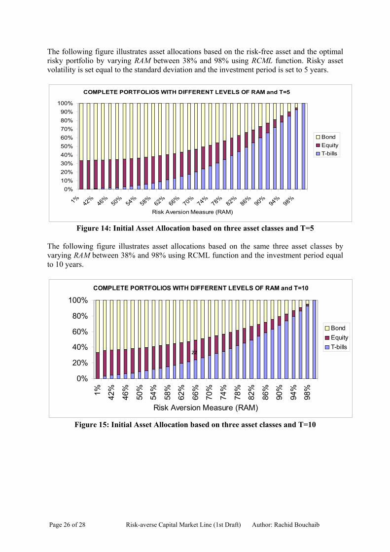
The following figure illustrates asset allocations based on the risk-free asset and the optimal risky portfolio by varying RAM between 38% and 98% using RCML function. Risky asset volatility is set equal to the standard deviation and the investment period is set to 5 years.
COMPLETE PORTFOLIOS WITH DIFFERENT LEVELS OF RAM and T=5
0%10%20%30%40%50%60%70%80%90%
100%
1%42%
46%50%
54%58%
62%66%
70%74%
78%82%
86%90%
94%98%
Risk Aversion Measure (RAM)
BondEquityT-bills
Figure 14: Initial Asset Allocation based on three asset classes and T=5
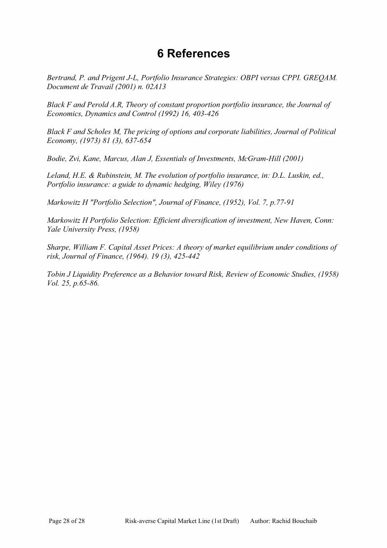
The following figure illustrates asset allocations based on the same three asset classes by varying RAM between 38% and 98% using RCML function and the investment period equal to 10 years.
COMPLETE PORTFOLIOS WITH DIFFERENT LEVELS OF RAM and T=10
0%
20%
40%
60%
80%
100%
1% 42%
46%
50%
54%
58%
62%
66%
70%
74%
78%
82%
86%
90%
94%
98%
Risk Aversion Measure (RAM)
BondEquityT-bills
zz
Figure 15: Initial Asset Allocation based on three asset classes and T=10
Page 26 of 28 Risk-averse Capital Market Line (1st Draft) Author: Rachid Bouchaib

5 Conclusion Risk-return combinations of all possible portfolios investing in the optimal risky portfolio and the risk-free asset give the capital market line. Selecting a complete portfolio from capital market line is a major asset allocation decision that current efficient portfolio theory has not yet addressed practically. This article has developed an analytical solution to the level of risky asset exposure based on a downside risk framework using option replication techniques. Combining ROBPI’s result with Markowitz’s efficient risky portfolio leads to an analytical solution of complete portfolio selection in a downside risk framework. The analytical solution RCML function depends on three parameters Risk Aversion Measure, investment period, and risky volatility. Using Risk-averse Capital Market Line function with combinations of RAMs and investment periods give complete portfolios in the same Capital Market Line. Asset allocations of complete portfolios and CML’s tangent depend on the level of risky asset volatility. RCML function is derived from Black & Scholes’ option formula of Call spread strategies. It goes beyond traditional portfolio insurance techniques as it allows more option strategies and can be used to derive Risk Aversion Measure related to asset allocation decisions.
Page 27 of 28 Risk-averse Capital Market Line (1st Draft) Author: Rachid Bouchaib
Page 28 of 28 Risk-averse Capital Market Line (1st Draft) Author: Rachid Bouchaib
6 References Bertrand, P. and Prigent J-L, Portfolio Insurance Strategies: OBPI versus CPPI. GREQAM. Document de Travail (2001) n. 02A13 Black F and Perold A.R, Theory of constant proportion portfolio insurance, the Journal of Economics, Dynamics and Control (1992) 16, 403-426 Black F and Scholes M, The pricing of options and corporate liabilities, Journal of Political Economy, (1973) 81 (3), 637-654 Bodie, Zvi, Kane, Marcus, Alan J, Essentials of Investments, McGram-Hill (2001)
Leland, H.E. & Rubinstein, M. The evolution of portfolio insurance, in: D.L. Luskin, ed., Portfolio insurance: a guide to dynamic hedging, Wiley (1976) Markowitz H "Portfolio Selection", Journal of Finance, (1952), Vol. 7, p.77-91 Markowitz H Portfolio Selection: Efficient diversification of investment, New Haven, Conn: Yale University Press, (1958) Sharpe, William F. Capital Asset Prices: A theory of market equilibrium under conditions of risk, Journal of Finance, (1964). 19 (3), 425-442 Tobin J Liquidity Preference as a Behavior toward Risk, Review of Economic Studies, (1958) Vol. 25, p.65-86.