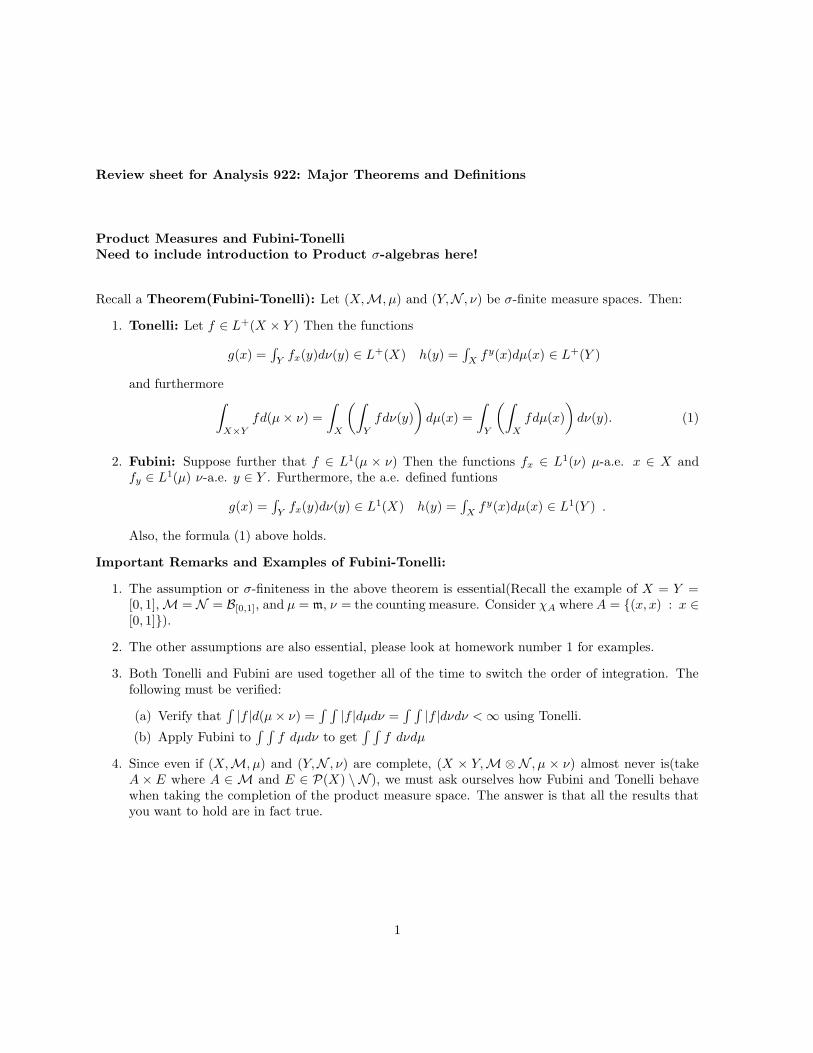
Review sheet for Analysis 922: Major Theorems and Definitions

Product Measures and Fubini-TonelliNeed to include introduction to Product σ-algebras here!

Recall a Theorem(Fubini-Tonelli): Let (X,M, µ) and (Y,N , ν) be σ-finite measure spaces. Then:

1. Tonelli: Let f ∈ L+(X × Y ) Then the functions

g(x) =∫

Y fx(y)dν(y) ∈ L+(X) h(y) =∫

X fy(x)dµ(x) ∈ L+(Y )

and furthermore∫

X×Y

fd(µ× ν) =

∫

X

(∫

Y

fdν(y)

)

dµ(x) =

∫

Y

(∫

X

fdµ(x)

)

dν(y). (1)

2. Fubini: Suppose further that f ∈ L1(µ × ν) Then the functions fx ∈ L1(ν) µ-a.e. x ∈ X andfy ∈ L1(µ) ν-a.e. y ∈ Y . Furthermore, the a.e. defined funtions

g(x) =∫

Yfx(y)dν(y) ∈ L1(X) h(y) =

∫

Xfy(x)dµ(x) ∈ L1(Y ) .

Also, the formula (1) above holds.

Important Remarks and Examples of Fubini-Tonelli:

1. The assumption or σ-finiteness in the above theorem is essential(Recall the example of X = Y =[0, 1], M = N = B[0,1], and µ = m, ν = the counting measure. Consider χA where A = (x, x) : x ∈[0, 1]).

2. The other assumptions are also essential, please look at homework number 1 for examples.

3. Both Tonelli and Fubini are used together all of the time to switch the order of integration. Thefollowing must be verified:

(a) Verify that∫

|f |d(µ× ν) =∫ ∫

|f |dµdν =∫ ∫

|f |dνdν <∞ using Tonelli.

(b) Apply Fubini to∫ ∫

f dµdν to get∫ ∫

f dνdµ

4. Since even if (X,M, µ) and (Y,N , ν) are complete, (X × Y,M ⊗ N , µ × ν) almost never is(takeA × E where A ∈ M and E ∈ P(X) \ N ), we must ask ourselves how Fubini and Tonelli behavewhen taking the completion of the product measure space. The answer is that all the results thatyou want to hold are in fact true.

1

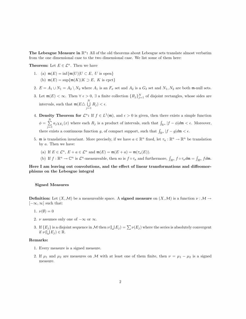
The Lebesgue Measure in Rn: All of the old theorems about Lebesgue sets translate almost verbatimfrom the one dimensional case to the two dimensional case. We list some of them here:

Theorem: Let E ∈ Ln. Then we have

1. (a) m(E) = infm(U)|U ⊂ E, U is open

(b) m(E) = supm(K)|K ⊃ E, K is cpct

2. E = A1 ∪N1 = A2 \N2 where A1 is an Fσ set and A2 is a Gδ set and N1, N2 are both m-null sets.

3. Let m(E) < ∞. Then ∀ ε > 0, ∃ a finite collection RjNj=1 of disjoint rectangles, whose sides are

intervals, such that m(E4N⋃

j=1

Rj) < ε.

4. Density Theorem for Ln: If f ∈ L1(m), and ε > 0 is given, then there exists a simple function

φ =N∑

j=1

ajχEj(x) where each Rj is a product of intervals, such that

∫

Rn |f − φ|dm < ε. Moreover,

there exists a continuous function g, of compact support, such that∫

Rn |f − g|dm < ε.

5. m is translation invariant. More precisely, if we have a ∈ Rn fixed, let τa : Rn → Rn be translationby a. Then we have:

(a) If E ∈ Ln, E + a ∈ Ln and m(E) = m(E + a) = m(τa(E)).

(b) If f : Rn → Cn is Ln-measureable, then so is f τa and furthermore,∫

Rn f τadm =∫

Rn fdm.

Here I am leaving out convolutions, and the effect of linear transformations and diffeomor-phisms on the Lebesgue integral

Signed Measures

Definition: Let (X,M) be a measureable space. A signed measure on (X,M) is a function ν : M →[−∞,∞] such that:

1. ν(∅) = 0

2. ν assumes only one of −∞ or ∞.

3. If Ej is a disjoint sequence in M then ν(⋃

Ej) =∑

ν(Ej) where the series is absolutely convergentif ν(

⋃

Ej) ∈ R.

Remarks:

1. Every measure is a signed measure.

2. If µ1 and µ2 are measures on M with at least one of them finite, then ν = µ1 − µ2 is a signedmeasure.

2

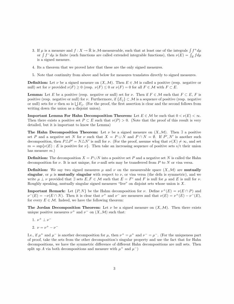
3. If µ is a measure and f : X → R is M-measureable, such that at least one of the integrals∫

f+dµor∫

f−dµ is finite (such functions are called extended integrable functions), then ν(E) =∫

E fdµis a signed measure.

4. Its a theorem that we proved later that these are the only signed measures.

5. Note that continuity from above and below for measures translates directly to signed measures.

Definition: Let ν be a signed measure on (X,M). Then E ∈ M is called a positive (resp. negative ornull) set for ν provided ν(F ) ≥ 0 (resp. ν(F ) ≤ 0 or ν(F ) = 0 for all F ∈ M with F ⊂ E.

Lemma: Let E be a positive (resp. negative or null) set for ν. Then if F ∈ M such that F ⊂ E, F ispositive (resp. negative or null) for ν. Furthermore, if Ej ⊂ M is a sequence of positive (resp. negativeor null) sets for ν then so is

⋃

Ej . (For the proof, the first assertion is clear and the second follows fromwriting down the union as a disjoint union).

Important Lemma For Hahn Decomposition Theorem: Let E ∈ M be such that 0 < ν(E) <∞.Then there exists a positive set P ⊂ E such that ν(P ) > 0. (Note that the proof of this result is verydetailed, but it is important to know the Lemma)

The Hahn Decomposition Theorem: Let ν be a signed measure on (X,M). Then ∃ a positiveset P and a negative set N for ν such that X = P ∪ N and P ∩ N = ∅. If P ′, N ′ is another suchdecomposition, then P4P ′ = N4N ′ is null for ν. (For the proof, assume wlog that ν(X) 6= ∞, and setm = supν(E) : E is positive for ν. Then take an increasing sequence of positive sets s/t their unionhas measure m.)

Definition: The decomposition X = P ∪N into a positive set P and a negative set N is called the Hahndecomposition for ν. It is not unique, for ν-null sets may be transferred from P to N or visa versa.

Definition: We say two signed measures µ and ν on the measureable space (X,M) are mutuallysingular, or µ is mutually singular with respect to ν, or visa versa (the defn is symmetric), and wewrite µ ⊥ ν provided that ∃ sets E,F ∈ M such that E = F c and F is null for µ and E is null for ν.Roughly speaking, mutually singular signed measures “live” on disjoint sets whose union is X .

Important Remark: Let P,N be the Hahm decomposition for ν. Define ν+(E) = ν(E ∩ P ) andν−(E) = −ν(E ∩ N). Then it is clear that ν+ and ν− are measures and that ν(E) = ν+(E) − ν−(E),for every E ∈ M. Indeed, we have the following theorem:

The Jordan Decomposition Theorem: Let ν be a signed measure on (X,M). Then there existsunique positive measures ν+ and ν− on (X,M) such that:

1. ν+ ⊥ ν−

2. ν = ν+ − ν−

I.e., if µ+ and µ− is another decomposition for µ, then ν+ = µ+ and ν− = µ−. (For the uniqueness partof proof, take the sets from the other decomposition’s singular property and use the fact that for Hahndecompositions, we have the symmetric difference of different Hahn decompositions are null sets. Thensplit up A via both decompositions and measure with µ+ and µ−)

3

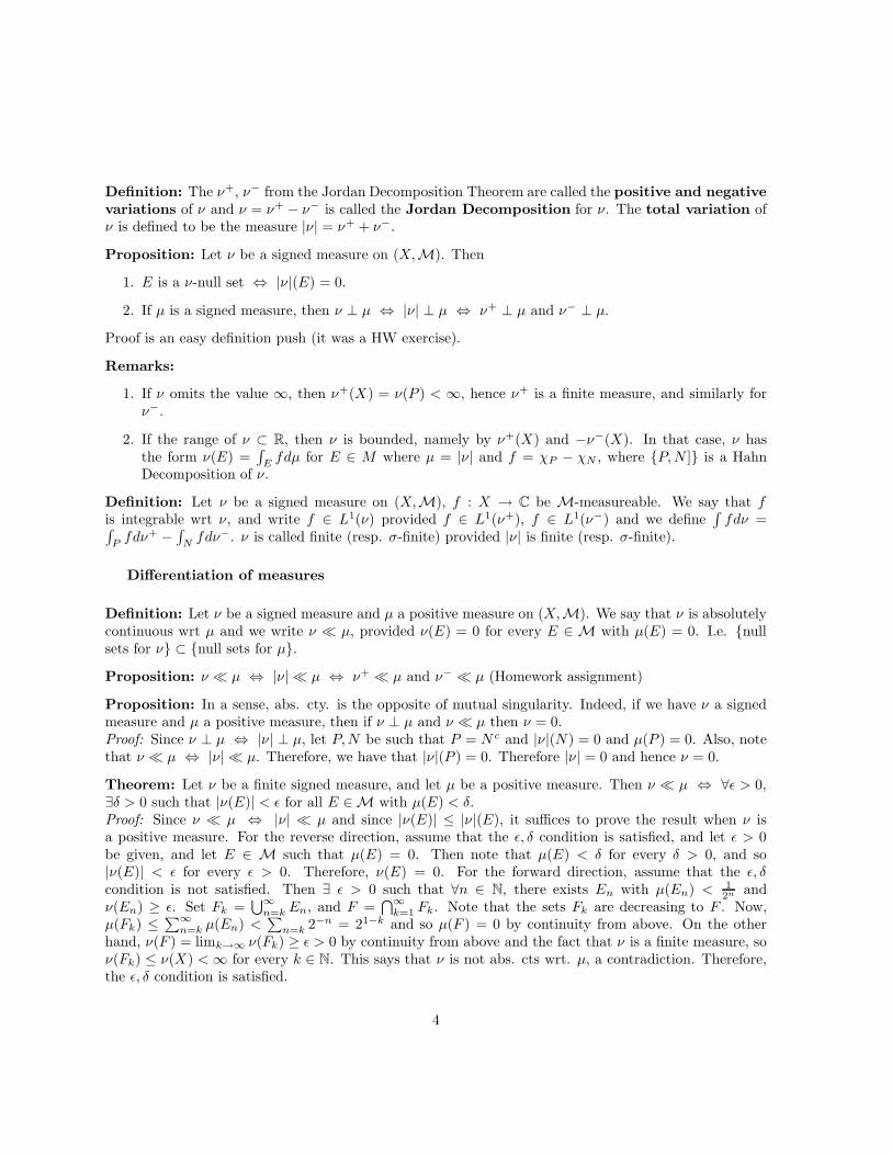
Definition: The ν+, ν− from the Jordan Decomposition Theorem are called the positive and negativevariations of ν and ν = ν+ − ν− is called the Jordan Decomposition for ν. The total variation ofν is defined to be the measure |ν| = ν+ + ν−.

Proposition: Let ν be a signed measure on (X,M). Then

1. E is a ν-null set ⇔ |ν|(E) = 0.

2. If µ is a signed measure, then ν ⊥ µ ⇔ |ν| ⊥ µ ⇔ ν+ ⊥ µ and ν− ⊥ µ.

Proof is an easy definition push (it was a HW exercise).

Remarks:

1. If ν omits the value ∞, then ν+(X) = ν(P ) < ∞, hence ν+ is a finite measure, and similarly forν−.

2. If the range of ν ⊂ R, then ν is bounded, namely by ν+(X) and −ν−(X). In that case, ν hasthe form ν(E) =

∫

E fdµ for E ∈ M where µ = |ν| and f = χP − χN , where P,N ] is a HahnDecomposition of ν.

Definition: Let ν be a signed measure on (X,M), f : X → C be M-measureable. We say that fis integrable wrt ν, and write f ∈ L1(ν) provided f ∈ L1(ν+), f ∈ L1(ν−) and we define

∫

fdν =∫

Pfdν+ −

∫

Nfdν−. ν is called finite (resp. σ-finite) provided |ν| is finite (resp. σ-finite).

Differentiation of measures

Definition: Let ν be a signed measure and µ a positive measure on (X,M). We say that ν is absolutelycontinuous wrt µ and we write ν µ, provided ν(E) = 0 for every E ∈ M with µ(E) = 0. I.e. nullsets for ν ⊂ null sets for µ.

Proposition: ν µ ⇔ |ν| µ ⇔ ν+ µ and ν− µ (Homework assignment)

Proposition: In a sense, abs. cty. is the opposite of mutual singularity. Indeed, if we have ν a signedmeasure and µ a positive measure, then if ν ⊥ µ and ν µ then ν = 0.Proof: Since ν ⊥ µ ⇔ |ν| ⊥ µ, let P,N be such that P = N c and |ν|(N) = 0 and µ(P ) = 0. Also, notethat ν µ ⇔ |ν| µ. Therefore, we have that |ν|(P ) = 0. Therefore |ν| = 0 and hence ν = 0.

Theorem: Let ν be a finite signed measure, and let µ be a positive measure. Then ν µ ⇔ ∀ε > 0,∃δ > 0 such that |ν(E)| < ε for all E ∈ M with µ(E) < δ.Proof: Since ν µ ⇔ |ν| µ and since |ν(E)| ≤ |ν|(E), it suffices to prove the result when ν isa positive measure. For the reverse direction, assume that the ε, δ condition is satisfied, and let ε > 0be given, and let E ∈ M such that µ(E) = 0. Then note that µ(E) < δ for every δ > 0, and so|ν(E)| < ε for every ε > 0. Therefore, ν(E) = 0. For the forward direction, assume that the ε, δcondition is not satisfied. Then ∃ ε > 0 such that ∀n ∈ N, there exists En with µ(En) < 1

2n andν(En) ≥ ε. Set Fk =

⋃∞n=k En, and F =

⋂∞k=1 Fk. Note that the sets Fk are decreasing to F . Now,

µ(Fk) ≤∑∞

n=k µ(En) <∑

n=k 2−n = 21−k and so µ(F ) = 0 by continuity from above. On the otherhand, ν(F ) = limk→∞ ν(Fk) ≥ ε > 0 by continuity from above and the fact that ν is a finite measure, soν(Fk) ≤ ν(X) <∞ for every k ∈ N. This says that ν is not abs. cts wrt. µ, a contradiction. Therefore,the ε, δ condition is satisfied.

4

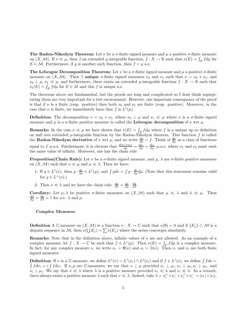
The Radon-Nikodym Theorem: Let ν be a σ-finite signed measure and µ a positive σ-finite measureon (X,M). If ν µ, then ∃ an extended µ-integrable function, f : X → R such that ν(E) =

∫

E fdµ forE ∈ M. Furthermore, if g is another such function, then f = g a.e.

The Lebesgue Decomposition Theorem: Let ν be a σ-finite signed measure and µ a positive σ-finitemeasure on (X,M). Then ∃ unique σ-finite signed measures ν0 and ν1 such that ν = ν0 + ν1, andν0 ⊥ µ, ν1 µ, and furthermore, there exists an extended µ-integrable function f : X → R such thatν1(E) =

∫

E fdµ for E ∈ M and this f is unique a.e.

The theorems above are fundamental, but the proofs are long and complicated so I dont think regurgi-tating them are very important for a test environment. However, one important consequence of the proofis that if ν is a finite (resp. positive) then both ν0 and ν1 are finite (resp. positive). Moreover, in thecase that ν is finite, we immediately have that f is L1(µ).

Definition: The decomposition ν = ν0 + ν1, where ν0 ⊥ µ and ν1 µ where ν is a σ-finite signedmeasure and µ is a σ-finite positive measure is called the Lebesgue decomposition of ν wrt µ.

Remarks: In the case ν µ we have shown that ν(E) =∫

Efdµ where f is a unique up to definition

on null sets extended µ-integrable function by the Radon-Nikodym theorem. This function f is calledthe Radon-Nikodym derivative of ν wrt µ, and we write dν

dµ = f . Think of dνdµ as a class of functions

equal to f µ-a.e. Furthermore, it is obvious that d(ν1+ν2)dµ = dν1

dµ + dν2

dµ µ-a.e, where ν1 and ν2 must omitthe same value of infinity. Moreover, one has the chain rule:

Proposition(Chain Rule): Let ν be a σ-finite signed measure, and µ, λ are σ-finite positive measureson (X,M) such that ν µ and µ λ. Then we have:

1. If g ∈ L1(ν), then g · dνdµ ∈ L1(µ), and

∫

gdν =∫

g · dνdµdµ. (Note that this statement remains valid

for g ∈ L+(ν).)

2. Then ν λ and we have the chain rule: dνdλ = dν

dµ · dµdλ .

Corollary: Let µ, λ be positive σ-finite measures on (X,M) such that µ λ and λ µ. Thendλdµ = dµ

dλ = 1 for a.e. λ and µ.

Complex Measures

Definition A C-measure on (X,M) is a function ν : X → C such that ν(∅) = 0 and if Ej ⊂ M is adisjoint sequence in M, then ν(

⋃

Ej) =∑

ν(Ej) where the series converges absolutely.

Remarks: Note that in the definition above, infinite values of ν are not allowed. As an example of acomplex measure, let f : X → C be such that f ∈ L1(µ). Then ν(E) =

∫

Efdµ is a complex measure.

In fact, for any complex measure ν, we write νr = <(ν) and νi = =(ν). Then νr and νi are both finitesigned measures.

Definition: If ν is a C-measure, we define L1(ν) = L1(νr) ∩ L1(νi) and if f ∈ L1(ν), we define∫

fdν =∫

fdνr + i∫

fdνi. If ν, µ are C-measures, we say that ν ⊥ µ provided νr ⊥ µr, νr ⊥ µi, νi ⊥ µr, andνi ⊥ µi. We say that ν λ where λ is a positive measure provided νr λ and νi λ. As a remark,there always exists a positive measure λ such that ν λ. Indeed, take λ = ν+

r +ν−r +ν+i +ν−i = |νr|+|νi|.

5

The Lebesgue-Radon-Nikodym Theorem for C-measures: Let ν be a C-measure, µ a σ-finitepositive measure on (X,M). Then ∃ a unique C-measures λ and ρ and f ∈ L1(µ) such that λ ⊥ µ, andρ µ, ν = λ+ ρ, where ρ(E) =

∫

Efdµ. If g is another such function, then f = g µ-a.e.

Definition: We define the total variation |ν| for a C-measure ν bu d|ν| = |f |dµ when ν µ anddν = fdµ where µ is a positive measure. The fact that this construction was well-defined was an exercise.

Properties of |ν|: Let ν be a C-measure on (X,M). Then

1. |ν(E)| ≤ |ν|(E), ∀ E ∈ M.

2. ν |ν| and∣

∣

∣

dνd|ν|

∣

∣

∣= 1 |ν|-a.e.

3. L1(ν) = L1(|ν|) and if f ∈ L1(ν) then∣

∣

∫

fdν∣

∣ ≤∫

|f |d|ν|.

4. If ν1 and ν2 are C-measures, then |ν1 + ν2| ≤ |ν1| + |ν2|.

Differentiation on Rn

Remember: Things to remember for the measures of balls in Rn: m(B(r, x)) = πn2 rn

Γ( n2+1) , and m(S(r, x)) =

0 where S(r, x) denotes the sphere in Rn of radius r centered at x.

Weiner’s Covering Lemma: Let C be a collection of open balls in Rn. Set U =⋃

B∈C B. If c < m(U),

then there exists disjoint B1, . . . , Bk ∈ C such thatk∑

i

m(Bj) > 3−nc. This lemma is used to prove several

results pertaining to differentiation in Rn.

Definition: A measureable function f : Rn → C is called locally integrable with respect to m provided∫

A |f |dm <∞ for every bounded set A ⊂ Ln. We set L1Loc

= f : Rn → C : f is measureable and locallyintegrable wrt m.

Definition: If f is locally integrable, we define its average value on B(r, x) by:

Arf(x) =1

m(B(r, x))

∫

B(r,x)

fdm

which is well defined for all x ∈ Rn, r > 0.

Lemma: If f ∈ L1Loc

(Rn), then Arf(x) is continuous on Rn × (0,∞), i.e. jointly in x and r.Proof: Recall that m(S(r, x)) = 0 for all x ∈ Rn and r > 0. Fix x0 ∈ Rn and r0 ∈ (0,∞), and letrk → r0 and xk → x0. Then we claim that χB(rk,xk)(y) → χB(r0,x0)(y) pointwise ∀ x ∈ Rn \ S(r0, x0).Indeed, fix y ∈ Rn \ S(r0, x0), and say that |y − x0| < r0, the outside the ball case being similar. Setε = r0 − |y − x0| > 0. So, there exists k0 ∈ N such that |rk − r0| <

ε2 and |xk − x0| <

ε2 for every k ≥ k0.

Now, for each k ≥ k0, we have |y−xk| ≤ |y−x0|+|x0−xk| < r0−ε+ε2 = r0−

ε2 < rk . Hence, y ∈ B(rk, xk),

and so χB(rk,xk)(y) = 1 = χB(r0,x0)(y) for k large enough. Therefore, we have shown that χB(rk,xk)(y) →

χB(r0,x0)(y) p.w.a.e. Now, choose k1 ∈ N such that rk < r0 + 12 and |xk − x0| <

12 for all k ≥ k1.

Then for all k ≥ k1 we have that B(rk , xk) ⊂ B(r0 + 1, x0), and hence |χB(rk,xk)(y)| ≤ χB(r0+1,x0)(y) ∈

6

L1(Rn,m). Now since f ∈ L1Loc

, then χB(rk,xk)(y)f(y)| ≤ χB(r0+1,x0)(y)|f(y)| ∈ L1(Rn), and furthermoreχB(rk,xk)(y)f(y) → χB(r0,x0)(y)f(y) p.w.a.e. So, by the Dominated Convergence Theorem, we have

limk→∞

∫

B(rk,xk)

f(y)dm =

∫

B(r0,x0)

f(y)dm.

This proves the result, since

Arkf(xk) =

1

m(B(rk , xk))

∫

B(rk,xk)

f(y)dm −→1

m(B(r0, x0))

∫

B(r0,x0)

f(y)dm = Arf(x).

Definition: Let f ∈ L1Loc

(Rn). We define its Hardy-Littlewood maximal function Hf(x), x ∈ Rn

by

Hf(x) = supr>0

Ar|f(x)| = supr>0

1

m(B(r, x))

∫

B(r,x)

|f(t)|dm(t)

By the last lemma, we have that the inverse image of the open rays is open, and so Hf is Borel-measureable, and hence is Ln measureable (indeed, we have that (Hf)−1(a,∞) =

⋃

r>0(Ar|f |)−1(a,∞),which is open in Rn.)

The Hardy-Littlewood Maximal Theorem: There exists C > 0 such that ∀f ∈ L1(m), and ∀α > 0,we have

m(x ∈ Rn : Hf(x) > α) ≤C

α

∫

Rn

|f |dm =C

α||f ||1

This proof is fairly reasonable, so should be looked at in detail. It involves the use of the Weiner coveringlemma.

Theorem: If f ∈ L1Loc

(Rn), then limr→0Arf(x) = f(x) m-a.e. x ∈ Rn.Notes: The proof of this theorem is very involved and uses the Hardy-Littlewood maximal thoerem. Don’texpect this on the exam, but its statement and use certainly are important. Note that this theorem impliesthat we have the following:

limr→0+

1

m(B(r, x))

∫

B(r,x)

(f(y) − f(x))dm(y) = 0 a.e.x ∈ Rn

We indeed have a stronger statement that we have yet to prove, where we replace f(y) − f(x) with|f(y) − f(x)|.

Definition: Let f ∈ L1Loc

(Rn). We define its Lebesgue Set to be:

Lf = x ∈ Rn : limr→0+

1

m(B(r, x))

∫

B(r,x)

|f(y) − f(x)|dm(y) = 0

Theorem: Let f ∈ L1Loc

(Rn). Then m(Lcf ) = 0.

Proof: Let c ∈ C. Set gc(x) = |f(x) − c|. So, gc(x) ∈ L1Loc

. So, by the previous theorem applied to gc(x),we have

limr→0+

1

m(B(r, x))

∫

B(r,x)

|f(y) − c|dm(y) = |f(x) − c| ∀x ∈ Rn \Ec

7

where Ec is a set of measure zero. Now, since C is separable (!), let cj be a countable dense subset ofC. So for each complex number we get a set of measure zero, and we have this countable dense subsetlieing around, so define E =

⋃∞j=1 Ecj

. Note that m(E) = 0. Fix x 6∈ E and let ε > 0 be given. Then∃ j ∈ N such that |cj − f(x)| < ε. Then we have

|f(y) − f(x)| ≤ |f(y) − cj | + |f(x) − cj | < |f(y) − cj | + ε

Hence, we have

lim supr→0+

1

m(B(r, x))

∫

B(r,x)

|f(y) − f(x)|dm(y) ≤

(

lim supr→0+

1

m(B(r, x))

∫

B(r,x)

|f(y) − cj |

)

+ ε.

This last integral, however, is equal to |f(x) − cj | + ε, as x 6∈ E, so we have the limit being less than 2εfor any ε > 0, so the limit must be 0. Therefore, x ∈ Lf . Therefore, we have Ec ⊂ Lf , hence E ⊃ Lc

f .Therefore, since m(E) = 0, we must have that m(Lc

f ) = 0.

Definition: A family Err>0 ⊂ BRn is said to shrink nicely at x provided

1. Er ⊂ B(r, x)∀r > 0

2. ∃α > 0 such that m(Er) > αm(B(r, x)) for all r > 0.

The Lebesgue Differentiation Theorem: Let f ∈ L1Loc

(Rn). Then for all x ∈ Lf we have

limr→0

1

m(Er)

∫

Er

|f(y) − f(x)|dm(y) = 0

and

limr→0

1

m(Er)

∫

Er

f(y)dm(y) = f(x)

for every family Er that shrinks nicely at x.Proof: The key point to notice is that we’ve rigged the definition of “family that shrinks nicely to x” sothat the proof of this result is basically already done for us. So, let x ∈ Lf be fixed. By definition, wehave that Er ⊂ B(r, x) and ∃ α > 0 such that m(Er) > αm(B(r, x)). Then immediately, we have

0 ≤1

m(Er)

∫

Er

|f(y) − f(x)|dm(y) ≤1

αm(B(r, x))

∫

B(r,x)

|f(y) − f(x)|dm(y) → 0

as r → 0 since x ∈ Lf . So, the limit exists and is equal to zero for x ∈ Lf . The last statement follows aswe may remove the absolute values from the above and move f(x) outside and use definition of Arf(x).

Add the definition of derivative of a function wrt m

Definition: A Borel measure ν on Rn is called regular provided

1. ν(K) <∞ for all K ⊂ Rn, K compact.

2. ν(E) = infν(U)|U ⊃ E, U open, for all E ∈ BRn .

8

A signed or C-Borel measure ν is called regular provided |ν| is regular. As a remark, n = 1, 1) ⇒ 2) isan old theorem and its true for n > 1 as well, but we haven’t proved it. Note also that if ν is a regularmeasure, it already is σ-finite.

Example/Proposition: Let f ∈ L+(Rn) and ν(E) =∫

E fdm, E ∈ BRn , then ν is regular ⇔ f ∈L1

Loc(Rn).

Proof: Clearly f ∈ L1Loc

(Rn) ⇔ condition 1) holds above for ν to be regular. We will show 2). LetE ⊂ Rn be a bounded Borel set in Rn, and let ε > 0 be given. If G ⊃ E where G is open and bdd, andsince f ∈ L1

Loc, f ∈ L1(G,m). Then by a previous theorem, ∃δ > 0 such that

∫

Ffdm < ε ∀F ⊂ G with

F borel and m(F ) < δ. Recall that m(E) = infm(U) : U ⊃ E,U open. Then there exists an open setV such that V ⊃ E and m(E) + δ > m(V ). So, m(U) − m(E) < δ. Therefore m(U \ E) < δ. Hence∫

U\Efdm < ε. Or,

∫

Ufdm <

∫

Efdm+ ε, therefore ν(U) < ν(E)+ ε. Therefore, 2) above is valid when E

is bounded. Now chop up E into bounded pieces for the case where E is unbounded with finite measure(the infinite measure unbounded case is trivial).

Theorem A: Let ν be a regular signed of C-valued Borel measure on Rn, with dν = dλ + fdm whereλ ⊥ m. Then both dλ and fdm are regular and d|ν| = d|λ| + |f |dm.

Theorem B: Let λ be a signed or C-borel regular measure on Rn such that λ ⊥ m. Then for m-a.e.

x ∈ Rn we have limr→0λ(Er)m(Er) = 0 for every family Er that shringks nicely to x. (i.e. (Dλ)(x) = 0 a.e.

x ∈ Rn)

Theorem C: Combining theorems A and B and the Lebesgue Differentiation Theorem we have: Let νbe a regular signed or C-borel measure on Rn, and let dν = dλ + fdm be its Lebesgue-Radon-Nikodymdecomposition wrt m. Then for m-a.e. x ∈ Rn,

limr→0

ν(Er)

m(Er)= f(x)

for every family Er that shrinks nicely to x. Hence (Dν)(x) = f(x) m-a.e. x ∈ Rn.

Applications of the Lebesgue Diff. Theorem to functions of Bounded Variations

Theorem 1: Let F : R → R be a nondecreasing function. Let G(x) = F (x+) = limy→x+ F (y). Then

1. F is cts on R except at possibly finitely many points, and

2. F and G are differentiable a.e. and F ′ = G′ a.e.

Definition: Let F : R → C. Fix an x ∈ R and let Px be a partition of the form Px = x0 < x1 < · · · <xn−1 < xn = x. Denote Px to be the collection of all such partitions. For each partition Px, defineS(Px, F ) by:

S(Px, F ) =

n∑

j=1

|F (xj) − F (xj−1)|

Define the total variation function of F by:

TF (x) = supPx∈Px

S(Px, F )

9

Remarks:

1. Note that if Px ⊂ Px, then S(Px, F ) ≤ S(Px, F ). In particular, if a < b, let Pb ∈ Pb and letPb = Pb ∪ b (and let Pb be the collection of all such partitions of this form). Then note thatPb ⊂ Pb since Pb is just the collection of all partitions of b such that a is included. Therefore,we have supPb∈Pb

S(Pb, F ) ≥ supPb∈PbS(Pb, F ). However, S(Pb, F ) ≤ S(Pb, F ) for all Pb, so

supPb∈PbS(Pb, F ) ≤ supPb∈Pb

S(Pb, F ), proving that specifying a finite number of points in thepartition does not alter the calculation of TF (b).

2. Also, if a < b then TF (b) = supP∈P[a,b] S(P, F )+TF (a). In particular, we have that TF (b)−TF (a) =supP∈P[a,b] S(P, F ) ≥ 0. Therefore TF is a nondecreasing function, with values in [0,∞].

3. As a matter of notation, we define TF (−∞) = limx→−∞ TF (x) and TF (∞) = limx→∞ TF (x).

Definition: If TF (∞) <∞, then F is said to be of bounded variation and we denote it by F ∈ BV .So, the space BV is defined by:

BV = F : R → C : F is of bounded variation, i.e. TF (∞) <∞

Also, we define the total variation of F on [a, b] to be TF (b)−TF (a). We denote by BV [a, b] the space of allfunctions that are of bounded total variation on [a, b]. Clearly, if F ∈ BV , we have that F |[a, b] ∈ BV [a, b].Conversely, if F ∈ BV [a, b], we may extend F to an element in BV as follows: F (x) = F (a) ∀ x < a,F (x) = F (b) ∀x > b (i.e. constant outside [a, b]).

Examples:

1. If F : R → R is bounded and increasing, then F ∈ BV . Indeed, set x = b and y = a such that a < b,and let P ∈ P [a, b]. Then S(P, F ) =

∑

|F (xj)−F (xj−1)| =∑

(F (xj)−F (xj−1)) = F (b)−F (a) =F (x) − F (y). So, TF (x) = supPx∈Px

S(Px, F ) = F (x) − F (−∞) ≤ F (∞) − F (−∞) <∞.

2. Suppose F,G ∈ BV and a, b ∈ C. The aF + bG ∈ BV so that BV is a linear space over C.

3. Suppose F : R → C is differentiable and F ′ is bounded on R. Then F ∈ BV [a, b] for any a < b.Indeed, let P ∈ P [a, b]. Then by the mean value theorem, we have that S(P, F ) =

∑

|F (xj) −F (xj−1)| =

∑

|F ′(tj)|(xj−xj−1) ≤M∑

(xj−xj−1) = M(b−a). So, TF (b)−TF (a) ≤M(b−a) <∞,hence F ∈ BV [a, b].

4. If F (x) = sin(x), then F ∈ BV [a, b] for every a < b but F is not BV .

5. If F (x) = x sin( 1x) for x 6= 0 and F (0) = 0, then F is not BV [a, b] for any a < b with 0 ∈ [a, b].

Lemma: If F ∈ BV is R-valued, then TF + F and TF − F are nondecreasing on R (the same statementis valid on [a, b]).

Remark: Let F ∈ BV , Im(F ) ⊂ R. Then F = 12 (TF + F ) − 1

2 (TF − F ), which is the difference of twoincreasing functions. In fact, we have this as part of the following theorem.

Theorem:

1. F ∈ BV ⇔ <(F ) ∈ BV and =(F ) ∈ BV .

10

2. Let F : R → R. Then F ∈ BV ⇔ F is the difference of two increasing functions on R. Indeed,F = 1

2 (TF + F ) − 12 (TF − F ).

3. If F ∈ BV , then F (x+) and F (x−) exist ∀x ∈ R. In fact so does F (±∞).

4. If F ∈ BV , then the set at which F is discontinuous is at most countable.

5. If F ∈ BV and G(x) = F (x+), then both F ′ and G′ exist and F ′ = G′ a.e.

Definition: Let F : R → R such that F ∈ BV . The decomposition F = 12 (TF +F )− 1

2 (TF −F ) := F1−F2

is called the Jordan Decomposition of F , and F1 and F2 are called the positive and negative variationsof F .

Definition: Let NBV (Normalized Bounded Variation) be the space given by:

NBV := F ∈ BV : F is right continuous and F (−∞) = 0

Let F ∈ BV . Define G(x) = F (x+) − F (−∞). Then G(x) ∈ NBV . Also, G′ = F ′ a.e.

Lemma: Let F ∈ BV . Then

1. TF (−∞) = 0

2. If F is also right continuous, then TF (x) is right continuous as well.

Theorem:

1. Let µ be a C-Borel measure on R. Let F (x) = µ((−∞, x]). Then F ∈ NBV .

2. Conversely, if F ∈ NBV , then ∃ a unique C-Borel measure called µF such that F (x) = µF ((−∞, x]).Moreover |µF | = µTF

(this last statement is left as an exercise).

Proposition: If F ∈ NBV , then F ′ ∈ L1R

(m). Moreover,

1. µF ⊥ m ⇔ F ′ = 0 a.e.

2. µF m ⇔ F (x) =∫

(−∞,x] F′(y)dm(y).

Definition: A function F : R → C is called absolutely continuous if ∀ ε > 0, there exists δ > 0 suchthat for any finite set of disjoint intervals (aj , bj)N

j=1 (need not be open intervals) with∑N

1 (bj−aj) < δ,

then∑N

1 |F (bj) − F (aj)| < ε. F : [a, b] → C is absolutely continuous on [a, b] if the above holds for allchoices of (a, j, bj) ⊂ [a, b].

Remarks:

1. If F : R → C is absolutely continuous, then F is uniformly continuous. Converse is not true, forexample the Contor Function.

2. If F ′(x) exists and is bounded on R, then F is absolutely continuous. (choose δ = ε/M where Mis the bound for |F ′| and use the mean value theorem.

11

Proposition: Let F ∈ NBV . Then F is absolutely continuous ⇔ µF m. Proof is very long...

Corollary: If f ∈ L1(R,m), then F (x) =∫

(−∞,x] fdm ∈ NBV and F is absolutely continuous and F ′ = f

a.e. Conversely, if F ∈ NBV and F is absolutely continuous, then F ′ ∈ L1(R,m) and F =∫

(−∞,x] F′dm.

Lemma: If F is absolutely continuous on [a, b] then F ∈ BV [a, b].Proof: Let ε = 1. Then ∃ δ > 0 such that ∀ finite disjoint subintervals (aj , bj)N

j=1 of [a, b] such

that∑N

1 (bj − aj) < δ then∑

|F (bj) − F (aj)| < 1. Take N ∈ N so that b−aN < δ. Let P0 = a =

x0 < x1 < · · · < xN = b such that xj − xj−1 = b−aN . So, given any partition P ∈ P [a, b], say

P = a = t0 < t1 < · · · < tn = b. Set Pj = (P ∩ [xj−1, xj ])cupxj−1, xj. So, note that Pj ∈ P [xj−1, xj ],

and so∑N

j=1 S(Pj , F ) ≥ S(P, F ), but S(Pj , F ) =∑n

j=1 |F (ψj) − F (ψj−1)| < 1 by absolute continuity.Hence S(P, F ) < N , so that F ∈ BV [a, b].

The Fundamental Theorem of Calculus for Lebesgue Integrals: Let −∞ < a < b < ∞ andF : [a, b] → C be given. Then the following are equivalent:

1. F is absolutely continuous on [a, b].

2. F (x) − F (a) =∫

[a,x] fdm for x ∈ [a, b] for some f ∈ L1([a, b],m).

3. F is differentiable a.e. [a, b], F ′ ∈ L1([a, b],m) and F (x) − F (a) =∫

[a,x] F′dm, x ∈ [a, b].

Proof:

• 3) ⇒ 2): Trivial

• 2) ⇒ 1): Extend f as follows: f(x) = f(x) for x ∈ [a, b] and f(x) = 0 otherwise. Then f ∈ L1(m)on R. Furthermore,

∫

R|f |dm =

∫

[a,b]|f |dm < ∞. Define F (x) =

∫

(−∞,x]fdm. By the previous

corollary, F (x) is absolutely continuous on R, and F ′(x) = f a.e. on R. But for x ∈ [a, b],F =

∫

(−∞,a]fdm +

∫

[a,x]fdm =

∫

[a,x]fdm = F (x) − F (a). So F is absolutely continuous on [a, b],

because it is the sum of two absolutely continuous funtions, namely F (x) and F (a), and also notethat F ′ = F ′ = f a.e. on [a, b].

• 1) ⇒ 3): Assume F is absolutely continuous on [a, b]. Define G(x) = F (x) for x ∈ [a, b], andconstant from (−∞, a] and [b,∞), namely the value of F at a and b respectively. Set G(x) =G(x) − G(a). Then G is absolutely continuous on R, since G was, and therefore G ∈ NBV . Bythe last corollary, we have that G′(x) ∈ L1(R) and G =

∫

(−∞,x] G′dm. However, we know that

G′(x) = G′(x) = F ′(x) for a.e. x ∈ [a, b]. Hence F ′(x) ∈ L1([a, b]). Moreover, for x ∈ (a, b],F (x) − F (a) = G(x) =

∫

(−∞,x]G′dm =

∫

[a,x]F ′dm, by the definition of G above, which is what we

wished to prove.

As a side note, it is important to realize this is yet another characterization of absolute continuity.

Final Remarks:

1. Let µ be a C-Borel measure on Rn. Then µ is called discrete if ∃ a countable set xj ⊂ Rn anda sequence cj ⊂ C such that

∑

|cj | < ∞ and µ =∑∞

1 cjδxjwhere δxj

is the point mass at xj .On the other hand, µ is called continuous if µ(x) = 0 for all singletons x.

12

2. Any C-Borel measure µ can be written as µ = µd + µc where µd is discrete and µc is continuous.To prove this, let E = x ∈ Rn|µ(x) 6= 0. If F is a countable subset of E then the series∑

x∈F µ(x) converges absolutely by definition of a C-measure. Let Ek = x ∈ E : |µ(x)| >1/k. Note that Ek is a finite set for every k, since

∑

x∈Ekµ(x) = µ(Ek), and the series converges

absolutely. Hence, we have ∞ >∑

x∈Ek|µ(x)| >

∑

x∈Ek= 1

k card(Ek), and so card(Ek) is finite,and so E is at most countable. Now, set µd(A) = µ(A ∩ E), and µc(A) = µ(A ∩ Ec). Clearlyµ(A) = µd(A) + µc(A), for every A ∈ BRn . Furthermore, µd is discrete (µd =

∑

µ(xj)δxjfor

xj = E). Finally µc is continuous. Indeed, µc(x) = µ(x ∩ Ec) = 0.

3. If µ is discrete, then µ ⊥ m, and if µ m, then µ is continuous. Since µ = µd + µc, andµc = µsc+ µac where µsc ⊥ m and µac m. Then µ = µd + µsc + µac.

4. Notation: Let F ∈ NBV and µF be the unique C-Borel measure inherited by F (i.e.µF (−∞, x] =F (x), and µF (x, y] = F (y) − F (x). The following notation is useful:

∫

R

gdF =

∫

R

g(x)dF (x) =

∫

R

gdµF

Theorem (Integration by Parts Formula for Lebesgue-Stiljes Integrals: Let F,G ∈ NBV , andassume at least one of them is continuous. Then for −∞ < a < b <∞, we have:

∫

(a,b]

FdG+

∫

(a,b]

GdF = F (b)G(b) − F (a)G(a)

Baire Category (in Metric Spaces)

Definition: Let X be a metric space. A set E ⊂ X is called nowhere dense if E has empty interior

(i.e.

E= ∅). As an example, we have the Cantor Set, since C contains no open interval and C is closed.

Definition: Let E ⊂ X , X a metric space. We say E is of the first category if E is a countable unionof nowhere dense sets, i.e. E = ∪∞

i=1Ei with the Ei nowhere dense). Otherwise, E is of the secondcategory. For some examples, we have that in R, Q is first category since Q is countable and singlepoints are nowhere dense in R. Also, nowhere dense sets are first category, so the Cantor set is firstcategory.

Other examples: Let X = C[0, 1] be the set of all R-valued continuous functions on [0, 1], be endowedwith the metric d(f, g) = supx∈[0,1] |f(x)−g(x)|. Recall that fn → f in X ⇔ fn → f uniformly in [0, 1].

13

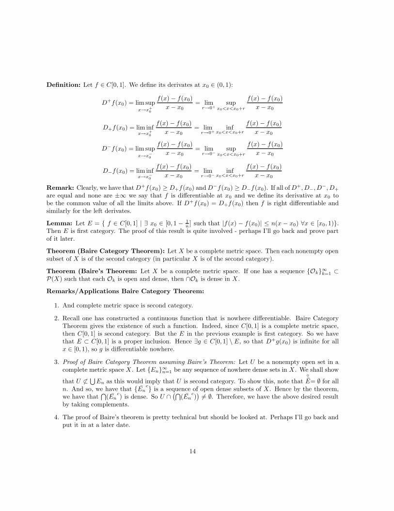
Definition: Let f ∈ C[0, 1]. We define its derivates at x0 ∈ (0, 1):

D+f(x0) = lim supx→x+

0

f(x) − f(x0)

x− x0= lim

r→0+sup

x0<x<x0+r

f(x) − f(x0)

x− x0

D+f(x0) = lim infx→x+

0

f(x) − f(x0)

x− x0= lim

r→0+inf

x0<x<x0+r

f(x) − f(x0)

x− x0

D−f(x0) = lim supx→x−

0

f(x) − f(x0)

x− x0= lim

r→0−

supx0<x<x0+r

f(x) − f(x0)

x− x0

D−f(x0) = lim infx→x−

0

f(x) − f(x0)

x− x0= lim

r→0−

infx0<x<x0+r

f(x) − f(x0)

x− x0

Remark: Clearly, we have thatD+f(x0) ≥ D+f(x0) andD−f(x0) ≥ D−f(x0). If all ofD+, D−, D−, D+

are equal and none are ±∞ we say that f is differentiable at x0 and we define its derivative at x0 tobe the common value of all the limits above. If D+f(x0) = D+f(x0) then f is right differentiable andsimilarly for the left derivates.

Lemma: Let E = f ∈ C[0, 1] | ∃ x0 ∈ [0, 1 − 1n ] such that |f(x) − f(x0)| ≤ n(x − x0) ∀x ∈ [x0, 1).

Then E is first category. The proof of this result is quite involved - perhaps I’ll go back and prove partof it later.

Theorem (Baire Category Theorem): Let X be a complete metric space. Then each nonempty opensubset of X is of the second category (in particular X is of the second category).

Theorem (Baire’s Theorem: Let X be a complete metric space. If one has a sequence Ok∞k=1 ⊂P(X) such that each Ok is open and dense, then ∩Ok is dense in X .

Remarks/Applications Baire Category Theorem:

1. And complete metric space is second category.

2. Recall one has constructed a continuous function that is nowhere differentiable. Baire CategoryTheorem gives the existence of such a function. Indeed, since C[0, 1] is a complete metric space,then C[0, 1] is second category. But the E in the previous example is first category. So we havethat E ⊂ C[0, 1] is a proper inclusion. Hence ∃g ∈ C[0, 1] \ E, so that D+g(x0) is infinite for allx ∈ [0, 1), so g is differentiable nowhere.

3. Proof of Baire Category Theorem assuming Baire’s Theorem: Let U be a nonempty open set in acomplete metric space X . Let En∞n=1 be any sequence of nowhere dense sets in X . We shall show

that U 6⊂⋃

En as this would imply that U is second category. To show this, note that

E= ∅ for alln. And so, we have that En

c is a sequence of open dense subsets of X . Hence by the theorem,

we have that⋂

(Enc) is dense. So U ∩

(⋂

(Enc))

6= ∅. Therefore, we have the above desired resultby taking complements.

4. The proof of Baire’s theorem is pretty technical but should be looked at. Perhaps I’ll go back andput it in at a later date.

14

As an immediate consequence of Baire’s Theorems, we have to following:Theorem: Uniform Boundedness Principle - Special Case: Let X be a complete metric space,and F 6= ∅ a collection of real-valued continuous functions on X . Assume that ∀x ∈ X , sup|f(x)| | f ∈F = Mx < ∞. Then there exists an open set U ⊂ X and a constant c > 0 such that |f(x)| ≤ c for allx ∈ U and for all f ∈ F .

Proof: For f ∈ F and m ∈ N, let Em,f = x ∈ X | |f(x) ≤ m. Clearly, Em,f is closed for every m andf . So, if we set Em =

⋂

f∈F Em,f , Em is closed. Furthermore, it is clear that X =⋃

Em where m ∈ N.So, since X is complete, not all of the Em can be nowhere dense as X is second category. So, there exists

m ∈ N such that

Em= Em 6= ∅. So, there exists an open set U ⊂ Em which does the job for us.

Final Remarks:

1. If E ⊂ X with X a metric space and E first category, then Ec = X \ E is called a residual set.First category sets are also sometimes called meager. Second category sets are called non-meagerand residual sets are sometimes called co-meager.

2. If O is open and F is closed then O \O and F \F are nowhere dense in X . If F is closed and firstcategory, and X is complete, then F is nowhere dense.

3. F is closed and nowhere dense if and only if F contains no nonempty open sets.

4. Let X be a complete metric space. Then E ⊂ X is residual ⇔ E contains a dense Gδ set. HenceE ⊂ X is first category if and only if E is a subset of F where F is an Fσ set such that F c is dense.

The Basic Theory Lp spaces and a bit on Duality and Separability

Definition: Let (X,M, µ) be a measure space fixed throughout. For an M measureable functionf : X → C, and 0 < p <∞ we define the p-norm of f to be:

‖f‖p :=

(∫

X

|f |pdµ

)1/p

∈ [0,∞]

We define the space Lp(X,M, µ) or Lp(X) or Lp(µ) or Lp to be:

Lp(X,M, µ) := f : X → C | f is M-measurable and ‖f‖p <∞

Note that as in L1, f = g in Lp if and only if f = g µ-almost everywhere. Also, if A is a nonempty setand µ is the counting measure on (A,P(A)), we denote lp to be Lp(A,P(A), µ). In the special case whereA = N, then lp(N) will simply be denoted lp and we have that:

lp =

an ⊂ C |

(

∞∑

n=1

|an|p

)1/p

<∞

15

Lemma: The following will be useful for our development of Lp spaces:

1. For a, b > 0 and 1 ≤ p <∞ we have that

(a+ b)p ≤ 2p−1(ap + bp)

2. For a, b > 0 and 0 < p < 1 then we have

(a+ b)p < ap + bp

Lemma: The above lemma shows that Lp is a vector space for any 0 < p <∞, as it gives the bound weneed on a sum of elements of Lp; linearity is easily verified.

Remark: The notation ‖f‖p suggests that ‖·‖p is a norm on Lp, i.e. it satisfies the following threeproperties:

1. ‖f‖p ≥ 0 for all f ∈ Lp(µ) and ‖f‖p = 0 if and only if f = 0 almost everywhere, which is clearlyvalid for all 0 < p <∞.

2. For every c ∈ C, we have that ‖cf‖p = |c| ‖f‖p, which is valid for all 0 < p <∞.

3. ∀ f, g ∈ Lp we should have ‖f + g‖p ≤ ‖f‖p +‖g‖p, the triangle inequality. However this is violatedfor 0 < p < 1 (Consider characteristic functions on positive measure sets that are disjoint and usethe above lemma).

Lemma(Young’s Inequality): The following is key to many results: Let a, b ≥ 0 and let 0 < λ < 1.Then we have

aλb1−λ ≤ λa+ (1 − λ)b

with equality if and only if a = b.Important remark: Young’s inequality often appears as follows: a, b ≥ 0, 1 < p < ∞ and let 1

p + 1q = 1

(i.e. (p, q) are Holder conjugates). Then ab ≤ ap

p + bq

q with equality if and only if ap = bq. The followingtheorem exploits this basic inequality for a powerful theorem:

Theorem (Holder’s Inequality:) Let 1 < p <∞, and 1p + 1

q = 1 be Holder conjugates. If f, g : X → C

are M-measureable, then we have

‖fg‖1 =

∫

X

|f ||g|dµ ≤ ‖f‖p ‖g‖q =

(∫

X

|f |p)1/p(∫

X

|g|q)1/q

In particular, f ∈ Lp and g ∈ Lq implies that fg ∈ L1, and in this case equality in the above holds if andonly if α|f |p = β|g|q , µ-a.e. for some α, β ≥ 0, but both not zero.Proof: If ‖f‖p = 0 or ‖g‖q = 0 then f = 0 a.e. or g = 0 a.e. so fg = 0 a.e. so the above is valid. Also,if either of the norms is ∞, again we have that the above is trivial. So, assume that 0 < ‖f‖p < ∞ and0 < ‖g‖p <∞. Then the above is valid if and only if the following inequality holds:

∫

|f ||g|

‖f‖p ‖g‖q

dµ ≤ 1

16

Set a = |f |‖f‖

p

and b = |g|‖g‖

q

. Then by Young’s Inequality we have:

|f |

‖f‖p

|g|

‖g‖q

≤|f |p

p ‖f‖pp

+|g|q

q ‖g‖qq

which is valid for all x ∈ X , with equality if and only if ap = bq. Integrating over X gives∫

X

|f |

‖f‖p

|g|

‖g‖q

dµ ≤1

p ‖f‖pp

∫

X

|f |p +1

q ‖g‖qq

∫

X

|g|q =1

p+

1

q= 1

with equality if and only if |f |p

‖f‖pp

= |g|q

‖g‖qq

, so the result is established by taking α = ‖g‖qq and β = ‖f‖p

p.

Note that Holder’s Inequality has immediate consequences: We can now prove the triangle inequality forthe p-norms when 1 ≤ p <∞, which is deemed Minkowski’s Inequality :

Theorem (Minkowski’s Inequality or Triangle Inequality for Lp): Let 1 ≤ p ≤ ∞, and f, g ∈ Lp.Then ‖f + g‖p ≤ ‖f‖p + ‖g‖q.

Proof: The proof is an application of Holder’s inequality twice with a = |f |, b = |f + g|p−1 and a′ = |g|,b′ = |f + g|p−1.

Definition: Let f : X → C be M-measureable. We define L∞ norm to be:

‖f‖∞ = infa ≥ 0|µx ∈ X | |f(x)| > a = 0

For such f , set Gf := a ≥ 0|µx ∈ X | |f(x)| > a = 0. Then ‖f‖∞ = inf Gf , with the conventionthat inf ∅ = ∞.

Remark: If Gf 6= ∅, then inf Gf = ‖f‖∞ := a0 ∈ Gf . Indeed, by definition we have that 0 ≤ a0 < ∞.So, there exists a sequence an ∈ Gf such that an ↓ a0. Set En = x ∈ X | |f(x)| > an. Thenµ(En) = 0. Also, En ⊂ En+1, as an+1 < an. And so, note that x ∈ X | |f(x)| > a0 =

⋃

En, and soµx ∈ X | |f(x)| > a0 = 0, hence a0 ∈ Gf .

Definition: We define the set of essentially bounded functions, L∞, to be

L∞ = L∞(X,M, µ) := f : X → C|f is M-measureable and ‖f‖∞ <∞.

Note again that we have f = g in L∞ if and only if f = g µ-almost everywhere.Remarks:

1. f ∈ L∞ ⇔ there exists a bounded measurable function g such that f = g almost everywhere µ.

2. If µ ν and ν µ then L∞(µ) = L∞(ν), and the norms also agree.

3. (L∞(µ), ‖·‖∞) is a normed space. He left the proof of this as an exercise that was not assigned - soit might be a good idea to take a look at it.

Definition: Let 1 ≤ p ≤ ∞. We say that fn ⊂ Lp converges to f in Lp (and we write fn → f inLp) provided ‖fn − f‖p → 0 as n→ ∞. fn is Cauchy in Lp if ‖fn − fm‖p → 0 as n,m→ ∞.

Theorem: If fn → f in Lp (0 < p < ∞), then there exists a subsequence fnj such that fnj

→ fpointwise almost everywhere.

17

Proof: Since∫

|fn − f |pdµ → 0 as n→ ∞, we have that |fn − f |p → 0 in L1. By an old theorem we havea subsequence such that |fnj

− f | → 0 µ-a.e. as j → ∞, as desired.

Definition: Let (X, ‖·‖) be a normed space. Let un ⊂ X . We say that un converges absolutely(or is absolutely convergent) in X if

∑

‖un‖ is convergent.

Theorem: A normed space (X, ‖·‖) is complete ⇔ Every absolutely convergent series in X converges inX . The proof is a little involved and really lives in the realm of functional analysis. Maybe I’ll go backin and type it out later.

Theorem (Reisz-Fisher): Lp is a Banach space (i.e. a complete normed space) for 1 ≤ p ≤ ∞.Proof: Omitted for now.

A Density Theorem for certain simple functions in Lp: Let 1 ≤ p ≤ ∞. Then the following set:

S := f =

n∑

j=1

ajχEj| µ(Ej) <∞

is dense in Lp. To prove this, use the old theorem on approximation of a measureable function by simplefunctions and note that if we are approximating a function in Lp, we must have that these simple functionsare in S.

Theorem (Facts about L∞:)

1. If f, g : X → C are M-measureable, then ‖fg‖1 ≤ ‖f‖1 ‖g‖∞. If f ∈ L1 and g ∈ L∞ then‖fg‖1 = ‖f‖1 ‖g‖∞ ⇔ |g(x)| = ‖g‖∞ a.e. on the set where f 6= 0.

2. ‖·‖∞ is a norm on L∞.

3. ‖fn − f‖∞ → 0 ⇔ ∃ a set E such that µ(Ec) = 0 and fn → f uniformly on E. Note that this isstrictly stronger than almost uniformly.

4. L∞ is a Banach space.

5. The simple functions are dense in L∞.

Proof: The proof of this result was also left as an exercise.

Theorem: If 0 < p < q < r ≤ ∞, then we have Lq ⊂ Lp + Lr (i.e. each f ∈ Lq may be written as thesum of an Lp function and an Lr function).Proof: Let f ∈ Lq. Set E = x ∈ X : |f(x)|| > 1, and let g = fχE and h = fχEc . Chearly we havef = g+h. Note also that we have chosen g and h appropriately so that the inequalities work and g ∈ Lp

and h ∈ Lr.

Theorem: If 0 < p < q < r <= ∞ then Lp ∩Lr ⊂ Lq, and futhermore, we have the following inequality:

‖f‖q ≤ ‖f‖λp ‖f‖1−λ

r

where λ is given by 1q = λ

p + 1−λr (actually, λ = q−1−r−1

p−1−r−1 ). The proof is a touchy Holder’s inequality

application with α = pλq and β = r

(1−λ)q . I’ll go back and type this up later.

18

Proposition: Let A be any nonempty set and µ be the counting measure on A. If 0 < p ≤ q ≤ ∞ thenlp(A) ⊂ lq(A) and ‖f‖q ≤ ‖f‖p.Proof: In this case, µ(E) = 0 ⇔ E = ∅. So, let f ∈ lp(A). Then we have that

‖f‖∞ =

(

supα∈A

|f(α)|

)p

= supα∈A

|f(α)|p ≤∑

α∈A

|f(α)|p = ‖f‖pp <∞.

Hence we have that lp(A) ⊂ l∞(A). So, suppose that q <∞. Then by the last theorem, with 0 < p < q <

r = ∞, we have that ‖f‖q ≤ ‖f‖λp ‖f‖1−λ

∞ and λ = pq . Therefore, we have that ‖f‖q ≤ ‖f‖p/q

p ‖f‖1−p/q∞ ≤

‖f‖p/qp ‖f‖1−p/q

p = ‖f‖p as desired.

Proposition: If µ(X) <∞ and 0 < p < q ≤ ∞ then Lq(µ) ⊂ Lp(µ) and ‖f‖p ≤ ‖f‖q µ(X)1p− 1

q .Proof: The q = ∞ case is almost trivial and for q <∞ you use Holder’s Inequality again thinking of |f |p

as 1 · |f |p with α = qp and β = q

q−p .

Final Remarks:

1. The most important Lp spaces are L1, L2 and L∞. L2 enjoys many fantastic properties seen later.L1 and L∞ are related, but studying practical problems is more fruitful to do in Lp where p is not1 or ∞.

2. A Banach space B is a normed space such taht the inherited metric is complete.

Duality in Lp spaces

Definition: Let X,Y be Banach spaces over a field F, where F is either the real or complex numbers.A linear mapping is called a linear operator from X to Y . We say a linear operator T : X → Y isbounded if ‖T‖ := supx∈X‖Tx‖ | ‖x‖ ≤ 1 < ∞. The set of all bounded linear operators from X toY is denoted L(X,Y ), with the understanding that L(X) = L(X,X).Remarks:

1. If T ∈ L(X,Y ), then it can be shown that the following equalities hold:

‖T‖ = supx∈X

‖Tx‖ | ‖x‖ ≤ 1

= sup‖x‖=1

‖Tx‖

= sup‖x‖6=0

‖Tx‖

‖x‖

= infc ≥ 0 | ‖Tx‖ ≤ c ‖x‖ ∀x ∈ X

Here, ‖T‖ is called the norm of the operator T .

2. If T ∈ L(X,Y ) then ‖Tx‖ ≤ ‖T‖ ‖x‖ for all x ∈ X , as is seen by the second equality applied tox

‖x‖ , which has norm 1.

19

3. If T ∈ L(X,Y ) then T (0) = 0.

Definition: A linear mapping T from X into F is called a linear functional.

Proposition: Let X,Y be normed spaces and T : X → Y be a linear operator. Then TFAE:

1. T is continuous at 0.

2. T is continuous at x for every x ∈ X .

3. T is bounded.

Proof: Will fill in later.

Remark: The special case when T ∈ L(X,F) where F is either R or C, i.e. T is a bounded linearfunctional on X , we have the definition of the norm of T is slightly simplified:

‖T‖ = supx6=0

|Tx|

‖x‖= sup

|x|=1

|Tx| = sup|x|≤1

|Tx|

= infc ≥ 0 | |Tx| ≤ c ‖x‖ ∀x ∈ X

Theorem (Duality of Lp spaces): Let 1 ≤ q < ∞ and 1p + 1

q = 1 and g ∈ Lq(µ) is fixed. Then

φg : Lp → C defined φg(f) =∫

fgdµ satisfies:

1. φg ∈ L(Lp,C)

2. ‖φg‖ = ‖g‖q .

In addition, if µ is semifinite, the same conclusions hold when q = ∞. In fact, we have a much strongerresult:

Theorem: Let 1 ≤ p, q ≤ ∞ be Holder conjugates. Let g : X → C be a fixed M-measureable functionsuch that fg ∈ L1 for all f ∈ Λ where Λ = simple functions that are identically zero on Ec withµ(E) < ∞, and assume that Mg := sup

∣

∣

∫

fgdµ∣

∣ : f ∈ Λ, ‖f‖p = 1 < ∞. Further, assume that eitherSg = x | g(x) 6= 0 is σ-finite or else assume µ is semifinite. Then g ∈ Lq(µ) and Mg = ‖g‖q .Proof : The proof of this result is highly technical.

Reisz Representation Theorem: Let 1 ≤ p <∞ and 1p + 1

q = 1. Assume that φ ∈ Lp(µ,C). Then

1. If 1 < p <∞ then ∃! g ∈ Lq(µ) such that φ(f) =∫

fgdµ and ‖φ‖ = ‖g‖q .

2. The same conclusions hold if p = 1 provided µ is σ-finite.

Proof: The proof of this result probably will not need to be reproduced.

Definition: The space of all bounded linear functionals on X , L(X,F) is called the dual space of X ,denoted X∗. So, in the case when X = Lp, we denote the space of all bounded linear functionals on Lp

taking values in C to be Lp(µ)∗.

Important Remarks:

20

1. For 1 ≤ p <∞ (and if p = 1 we also assume σ-finiteness of (X,µ), the mapping F : Lq(µ) → Lp(µ)∗

sending an Lq function to its functional is an isometric isomorphism. This means that it is a linearbijective continuous map that preserves norms and whose inverse is also continuous. Recall thatcontinuous is the same as bounded in this context.

2. The assertion that µ is σ-finite in the above theorem in the case that p = 1 and q = ∞ is essential.

3. The mapping F : L1(µ) → L∞(µ)∗ where g 7→ φg is always an isometric injection, but rarely asurjection.

Proof: First, note that C[0, 1] ⊂ L∞([0, 1]). Let us define φ : C[0, 1] → C by f 7→ f(0). Thenφ is clearly linear and the norm is 1. But you can use dominated convergence theorem to get acontradiction if you assume that there is an L1 function such that φ(f) =

∫

fgdµ.

Definition: Let X be a normed space over C or R and X∗ its dual. Then (X∗, ‖·‖) is a normed space,and in fact it is always a Banach space(!). We say a sequence xn ⊂ X converges weakly to x ∈ X iffor all φ ∈ X∗ we have φ(xn) → φ(x).

Theorem (Uniform Boundedness Principal, General Case): Let X,Y be normed spaces. LetTaa∈A ⊂ L(X,Y ) be a family of bounded linear operators from X to Y . Then

1. If supa∈A ‖Ta(x)‖ := Mx < ∞ for all x ∈ E where E is some second category set in X thensup ‖Ta‖ = M <∞.

2. If X is a Banach space, and if supa∈A ‖Ta(x)‖ := Mx < ∞, then sup ‖Ta‖ = M < ∞. Note that ifwe prove 1, part 2 follows immediately since X Banach implies that X is second category.

Proof: For n ∈ N, put En = x ∈ X | supa∈A ‖Ta(x)‖ ≤ n =⋂

a∈Ax ∈ X | ‖Ta(x)‖ ≤ n. ThenEn ⊂ En+1 and En is closed for all n (by continuity of Ta). Also, we have that

⋃∞n=1En ⊃ E so since E

is second category, ∃n0 ∈ N such that En0is second category. By an exercise, En0

contains a nonemptyopen set, say B(r, x0). So, En0

⊃ ¯B(r, x0) (note my puny attempt at a bar above the ball). I claimthat E2n0

⊃ ¯B(r, 0). Indeed, suppose ‖x‖ ≤ r. Then note that ‖x+ x0 − x0‖ = ‖x‖ ≤ r. Hence wehave that x + x0 ∈ ¯B(r, x0) ⊂ En0

. Hence, we have that ‖Ta(x+ x0)‖ ≤ n0, for all a ∈ A. So, we have‖Ta(x)‖ = ‖Ta(x + x0) − Ta(x0)‖ ≤ ‖Ta(x + x0)‖ + ‖Ta(x0)‖ ≤ 2n0. Therefore x ∈ E2n0

. So, we haveshown that for all x ∈ X with ‖x‖ ≤ r we have ‖Ta(x)‖ ≤ 2n0, for all a ∈ A. So, let x ∈ X such that‖x‖ ≤ 1. Then ‖rx‖ ≤ r. Thus, by the above, we have ‖Ta(x)‖ =

∥

∥

1rTa(rx)

∥

∥ ≤ 2n0

r for all a ∈ A. Hence,

‖Ta‖ = sup‖x‖≤1 ‖Ta(x)‖ ≤ 2n0

r for all a ∈ A. Hence we have that supa∈A ‖Ta‖ <∞, as desired.

Definition: Let X be a normed space and X∗ its dual. Then (X∗, ‖·‖) is a normed space. Infact, (X∗, ‖·‖) is a Banach space. We may consider X∗∗, the dual of X∗, where X∗∗ = L(X∗,C) =L(L(X,C),C). We call X∗∗ the double dual of X .For each x ∈ X we assign an element ψx ∈ X∗∗ such that ψx : X∗ → C is given by ψx(φ) 7→ φ(x).This is often called the evaluation map. Then we have that ‖ψx‖ = sup‖φ‖=1 |ψx(φ)| = sup‖φ‖=1 φ(x) ≤‖phi‖ ‖x‖ = ‖x‖. In fact, it can be shown that ‖ψx‖ = ‖x‖. So the mapping ψ is linear and an isometry.Therefore, ψ is an isometric isometry from X to ψ(X), which is a linear subspace of X∗∗. We say thatX is reflexive if ψ(X) = X∗∗.

Corollary to Reisz Representation Theorem: If 1 < p <∞, then Lp(µ) is reflexive.

21

Brief mention of Separability of Lp

Theorem (Stone-Weierstrauss): Let Ω = O, where O is an open bounded subset of Rn, and letA ⊂ C(Ω), where C(Ω) is the set of continuous functions on Ω. Then A is dense in C(Ω) provided Asatisfies:

1. A is an algebra (i.e. f, g ∈ A implies f + g, fg and cf ∈ A).

2. If f ∈ A then f ∈ A.

3. If x, y ∈ Ω, x 6= y then ∃f ∈ A such that f(x) 6= f(y).

4. If x ∈ Ω then ∃f ∈ A such that f(x) 6= 0.

Corollary: Let Ω be as above. Let Prat := all polynomials on Rn with rational complex coefficients.Then Prat is dense in C(Ω).

Corollary: C(Ω) where Ω is as above is separable.

Theorem: Lp(Rn,m) is separable, if 1 ≤ p <∞.Proof: Let Bj = B(j, 0) := x ∈ Rn | |x| ≤ j. Set Prat to be as above. Set Pj = χBj

Q | Q ∈ Prat.Then Pj is dense in C(Bj), and

⋃

Pj is countable. Let f ∈ Lp(Rn,m), and let ε > 0 be given. Then∃φ ∈ C0(Rn) such that ‖f − φ‖ < ε

3 , since the continuous functions of compact support are dense inLp. Say that φ = outside Bk for some k ∈ N. Now approximate φ with a polynomial Q in the abovecountable union of countable sets and playing with the triangle inequality gives you that ‖f −Q‖ < ε,as desired.

22