Review Finite Element Modeling - University of Massachusetts Lowell
44
1 Dr. Peter Avitabile Modal Analysis & Controls Laboratory 22.515 – Finite Element Review Review Finite Element Modeling Peter Avitabile Mechanical Engineering Department University of Massachusetts Lowell [ K ] n [ M ] n [ M ] a [ K ] a [ E ] a [ ω ] 2 Structural Dynamic Modeling Techniques & Modal Analysis Methods
Transcript of Review Finite Element Modeling - University of Massachusetts Lowell
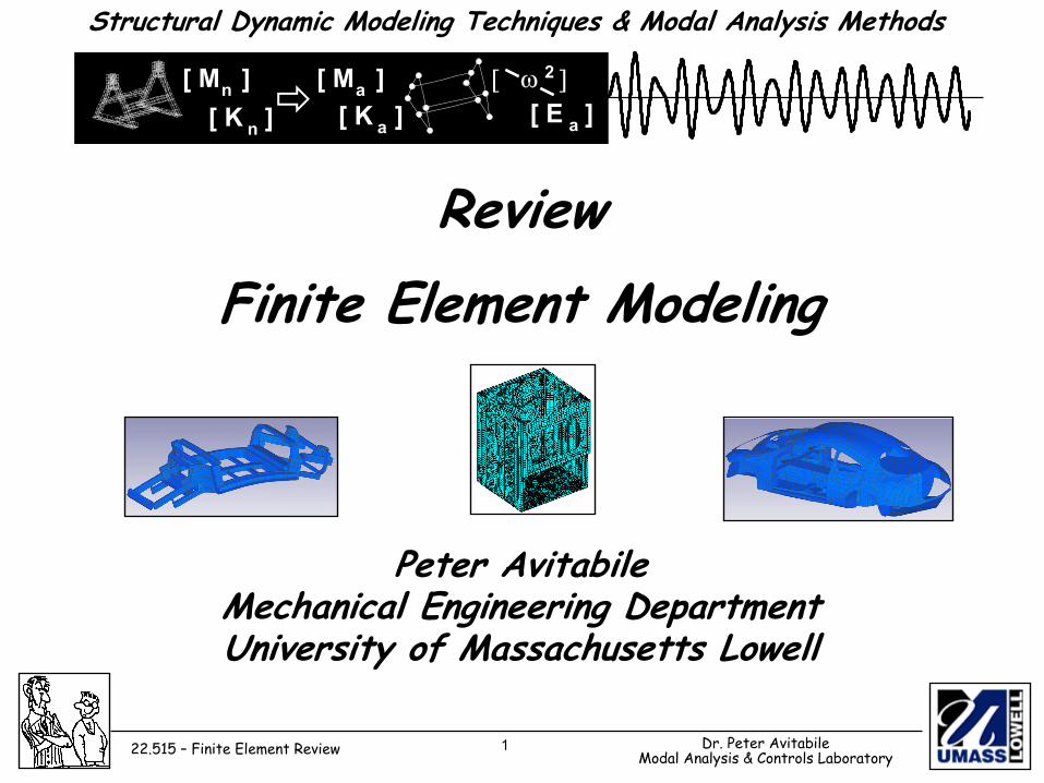
1 Dr. Peter AvitabileModal Analysis & Controls Laboratory22.515 – Finite Element Review
Review Finite Element Modeling
Peter AvitabileMechanical Engineering DepartmentUniversity of Massachusetts Lowell
[ K ]n
[ M ]n [ M ]a[ K ]a [ E ]a
[ ω ]2
Structural Dynamic Modeling Techniques & Modal Analysis Methods
2 Dr. Peter AvitabileModal Analysis & Controls Laboratory22.515 – Finite Element Review
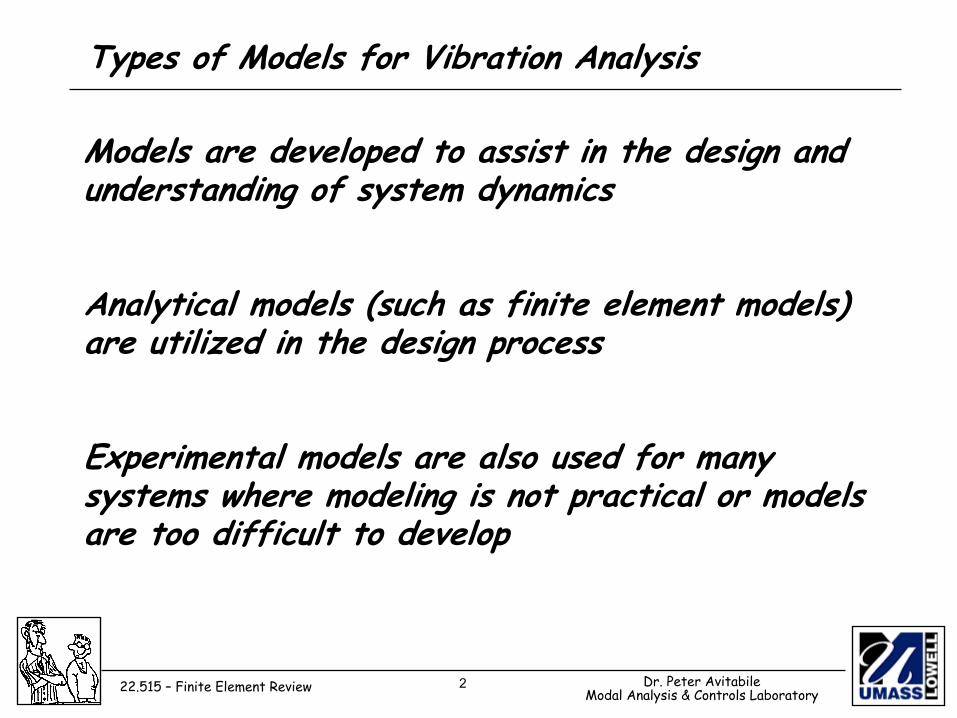
Types of Models for Vibration Analysis
Models are developed to assist in the design and understanding of system dynamics
Analytical models (such as finite element models) are utilized in the design process
Experimental models are also used for many systems where modeling is not practical or models are too difficult to develop
3 Dr. Peter AvitabileModal Analysis & Controls Laboratory22.515 – Finite Element Review
Finite Element Model Considerations
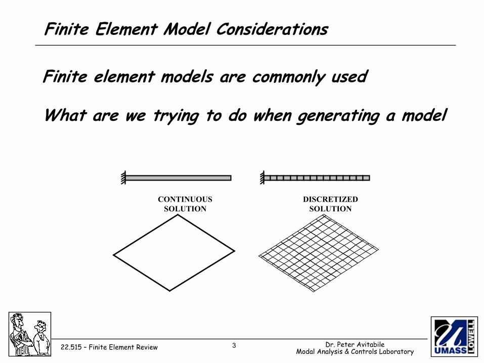
Finite element models are commonly used
What are we trying to do when generating a model
CONTINUOUS DISCRETIZED SOLUTION SOLUTION
4 Dr. Peter AvitabileModal Analysis & Controls Laboratory22.515 – Finite Element Review
Finite Element Model Considerations
Modeling Issues
• continuous solutions work well with structures that are well behaved and have no geometry that is difficult to handle
• most structures don't fit this simple requirement (except for frisbees and cymbals) • real structures have significant geometry variations that are
difficult to address for the applicable theory • a discretized model is needed in order to approximate the actual
geometry • the degree of discretization is dependent on the waveform of the
deformation in the structure • finite element modeling meets this need
5 Dr. Peter AvitabileModal Analysis & Controls Laboratory22.515 – Finite Element Review
Finite element modeling involves the descretization of the structure into elements or domains that are defined by nodes which describe the elements.
A field quantity such as displacement is approximated using polynomial interpolation over each of the domains.
The best values of the field quantity at nodes results from a minimization of the total energy.
Since there are many nodes defining many elements, a set of simultaneous equations results.
Typically, this set of equations is very large and a computer is used to generate results.
Finite Element Model Considerations
6 Dr. Peter AvitabileModal Analysis & Controls Laboratory22.515 – Finite Element Review
Finite Element Model Considerations
Nodes represent geometric locations in the structure.
Elements boundary are defined by the nodes.
The type of displacement field that exists over the domain will determine the type of element used to characterize the domain.
Element characteristics are determined from
Theory of Elasticity and
Strength of Materials.
7 Dr. Peter AvitabileModal Analysis & Controls Laboratory22.515 – Finite Element Review
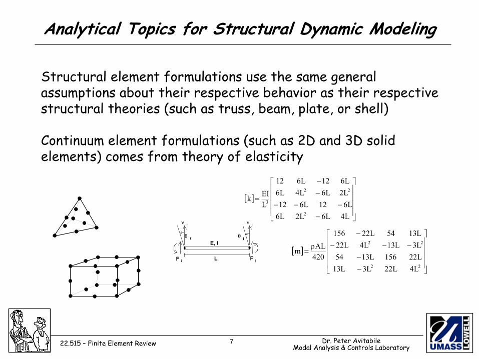
Analytical Topics for Structural Dynamic Modeling
Structural element formulations use the same general assumptions about their respective behavior as their respective structural theories (such as truss, beam, plate, or shell)
Continuum element formulations (such as 2D and 3D solid elements) comes from theory of elasticity
L
E, I
F F
θ i
i j
θ j
ν i ν j
[ ]
−−−−
−−
=
L4L6L2L6L612L612
L2L6L4L6L612L612
LEIk
2
22
3
[ ]
−−
−−−−
ρ=
22
22
L4L22L3L13L22156L1354L3L13L4L22L1354L22156
420ALm
8 Dr. Peter AvitabileModal Analysis & Controls Laboratory22.515 – Finite Element Review
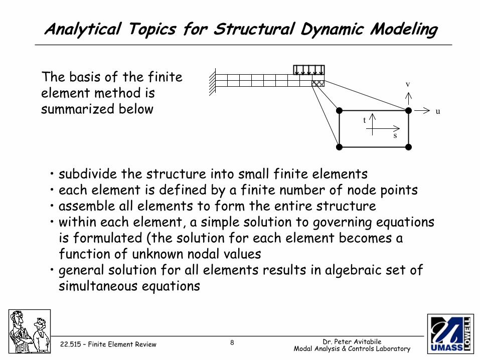
Analytical Topics for Structural Dynamic Modeling
The basis of the finite element method is summarized below
• subdivide the structure into small finite elements • each element is defined by a finite number of node points• assemble all elements to form the entire structure• within each element, a simple solution to governing equations
is formulated (the solution for each element becomes a function of unknown nodal values
• general solution for all elements results in algebraic set of simultaneous equations
u
v
s
t
9 Dr. Peter AvitabileModal Analysis & Controls Laboratory22.515 – Finite Element Review
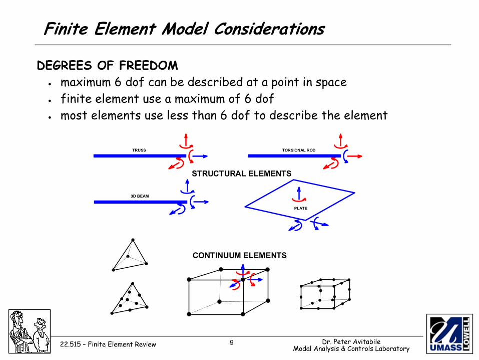
Finite Element Model Considerations
TRUSS
3D BEAM
PLATE
TORSIONAL ROD
STRUCTURAL ELEMENTS
CONTINUUM ELEMENTS
DEGREES OF FREEDOM • maximum 6 dof can be described at a point in space • finite element use a maximum of 6 dof • most elements use less than 6 dof to describe the element
10 Dr. Peter AvitabileModal Analysis & Controls Laboratory22.515 – Finite Element Review
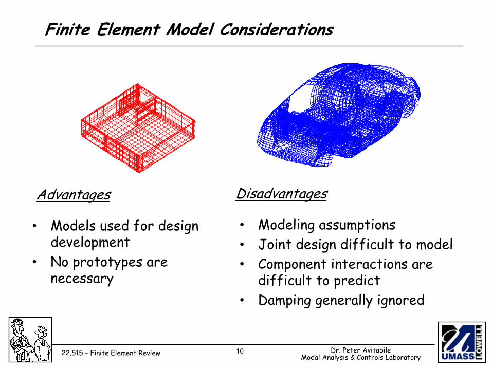
Finite Element Model Considerations
• Models used for design development
• No prototypes are necessary
• Modeling assumptions• Joint design difficult to model• Component interactions are
difficult to predict• Damping generally ignored
Advantages Disadvantages
11 Dr. Peter AvitabileModal Analysis & Controls Laboratory22.515 – Finite Element Review
Finite Element Model Considerations
A TYPICAL FINITE ELEMENT USER MAY ASK • what kind of elements should be used? • how many elements should I have? • where can the mesh be coarse; where must it be fine? • what simplifying assumptions can I make? • should all of the physical structural detail be included? • can I use the same static model for dynamic analysis? • how can I determine if my answers are accurate? • how do I know if the software is used properly?
12 Dr. Peter AvitabileModal Analysis & Controls Laboratory22.515 – Finite Element Review
Finite Element Model Considerations
ALL THESE QUESTIONS CAN BE ANSWERED, IF • the general structural behavior is well understood • the elements available are understood • the software operation is understood (input procedures, algorithms,etc.) BASICALLY - we need to know what we are doing !!!
IF A ROUGH BACK OF THE ENVELOP ANALYSIS CAN NOT BE FORMULATED, THEN
MOST LIKELY THE ANALYST DOES NOT KNOW ENOUGH ABOUT THE PROBLEM AT HAND TO
FORMULATE A FINITE ELEMENT MODEL
13 Dr. Peter AvitabileModal Analysis & Controls Laboratory22.515 – Finite Element Review
Finite Element Modeling
Using standard finite element modeling techniques, the following steps are usually followed in the generation of an analytical model
· node generation · element generation · coordinate transformations · assembly process · application of boundary conditions · model condensation · solution of equations · recovery process · expansion of reduced model results
14 Dr. Peter AvitabileModal Analysis & Controls Laboratory22.515 – Finite Element Review
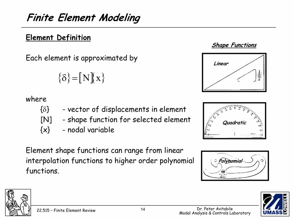
Element Definition Each element is approximated by where {δ} - vector of displacements in element [N] - shape function for selected element {x} - nodal variable Element shape functions can range from linear interpolation functions to higher order polynomial functions.
Finite Element Modeling
{ } [ ]{ }xN=δ
Shape Functions
Linear
Quadratic
Polynomial
15 Dr. Peter AvitabileModal Analysis & Controls Laboratory22.515 – Finite Element Review
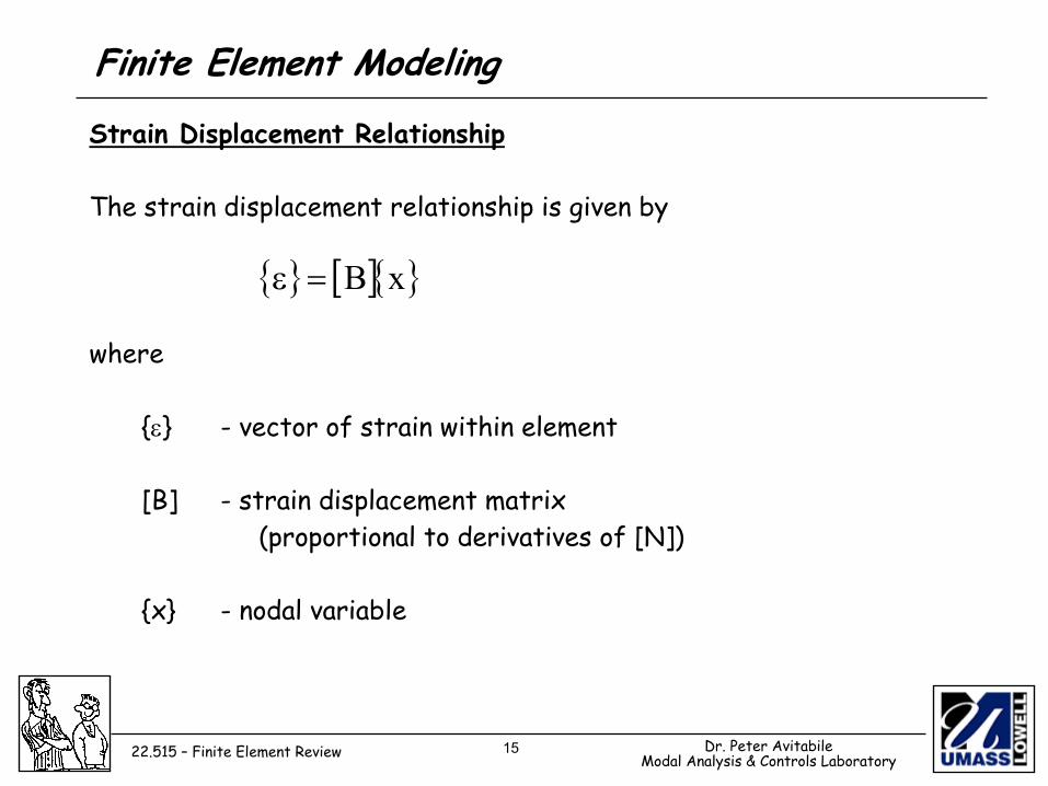
Strain Displacement Relationship The strain displacement relationship is given by where {ε} - vector of strain within element [B] - strain displacement matrix (proportional to derivatives of [N]) {x} - nodal variable
Finite Element Modeling
{ } [ ]{ }xB=ε
16 Dr. Peter AvitabileModal Analysis & Controls Laboratory22.515 – Finite Element Review
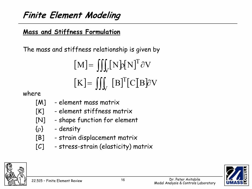
Mass and Stiffness Formulation The mass and stiffness relationship is given by where [M] - element mass matrix [K] - element stiffness matrix [N] - shape function for element {ρ} - density [B] - strain displacement matrix [C] - stress-strain (elasticity) matrix
Finite Element Modeling
[ ] [ ] [ ]
[ ] [ ] [ ][ ] VBCBK
VNNM
TV
TV
∂=
∂ρ=
∫∫∫∫∫∫
17 Dr. Peter AvitabileModal Analysis & Controls Laboratory22.515 – Finite Element Review
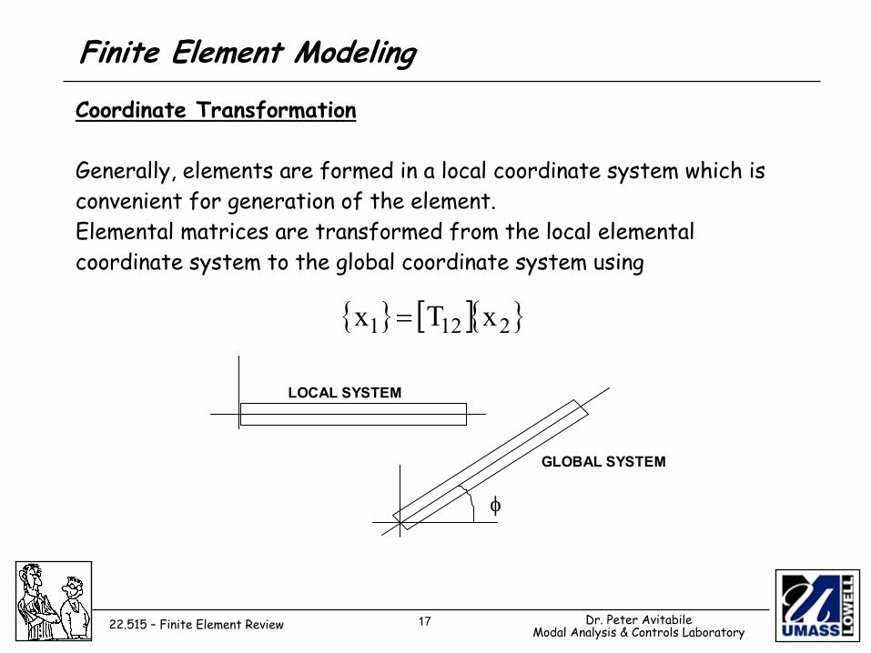
Coordinate Transformation Generally, elements are formed in a local coordinate system which is convenient for generation of the element. Elemental matrices are transformed from the local elemental coordinate system to the global coordinate system using
Finite Element Modeling
{ } [ ]{ }2121 xTx =
LOCAL SYSTEM
GLOBAL SYSTEM
φ
18 Dr. Peter AvitabileModal Analysis & Controls Laboratory22.515 – Finite Element Review
Finite Element Modeling
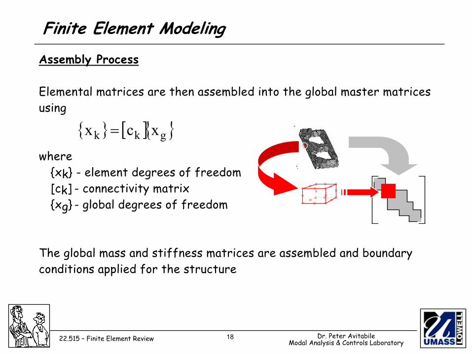
{ } [ ]{ }gkk xcx =
Assembly Process
Elemental matrices are then assembled into the global master matricesusing
where{xk} - element degrees of freedom[ck] - connectivity matrix{xg} - global degrees of freedom
The global mass and stiffness matrices are assembled and boundaryconditions applied for the structure
19 Dr. Peter AvitabileModal Analysis & Controls Laboratory22.515 – Finite Element Review
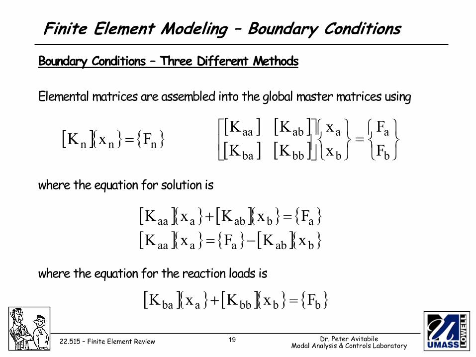
Boundary Conditions – Three Different Methods Elemental matrices are assembled into the global master matrices using where the equation for solution is where the equation for the reaction loads is
Finite Element Modeling – Boundary Conditions
[ ]{ } { }nnn FxK =[ ] [ ][ ] [ ]
=
b
a
b
a
bbba
abaa
FF
xx
KKKK
[ ]{ } [ ]{ } { }[ ]{ } { } [ ]{ }babaaaa
ababaaa
xKFxKFxKxK
−==+
[ ]{ } [ ]{ } { }bbbbaba FxKxK =+
20 Dr. Peter AvitabileModal Analysis & Controls Laboratory22.515 – Finite Element Review
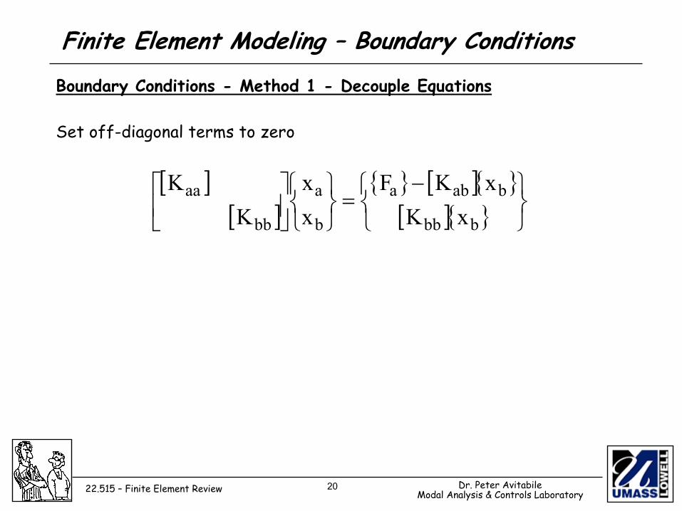
Boundary Conditions - Method 1 - Decouple Equations Set off-diagonal terms to zero
Finite Element Modeling – Boundary Conditions
[ ][ ]
{ } [ ]{ }[ ]{ }
−
=
bbb
baba
b
a
bb
aa
xKxKF
xx
KK
21 Dr. Peter AvitabileModal Analysis & Controls Laboratory22.515 – Finite Element Review
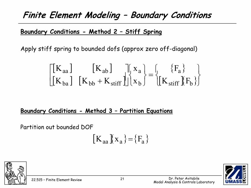
Boundary Conditions - Method 2 – Stiff Spring Apply stiff spring to bounded dofs (approx zero off-diagonal)
Finite Element Modeling – Boundary Conditions
[ ] [ ][ ] [ ]
{ }[ ]{ }
=
+ bstiff
a
b
a
stiffbbba
abaa
FKF
xx
KKKKK
Boundary Conditions - Method 3 – Partition Equations Partition out bounded DOF
[ ]{ } { }aaaa FxK =
22 Dr. Peter AvitabileModal Analysis & Controls Laboratory22.515 – Finite Element Review
Finite Element Modeling
Static Solutions• typically involve decomposition of a large matrix• matrix is usually sparsely populated• majority of terms concentrated about the diagonal
Eigenvalue Solutions• use either direct or iterative methods• direct techniques used for small matrices• iterative techniques used for a few modes from large matrices
Propagation Solutions• most common solution uses derivative methods• stability of the numerical process is of concern• at a given time step, the equations are reduced to an equivalent
static form for solution• typically many times steps are required
23 Dr. Peter AvitabileModal Analysis & Controls Laboratory22.515 – Finite Element Review
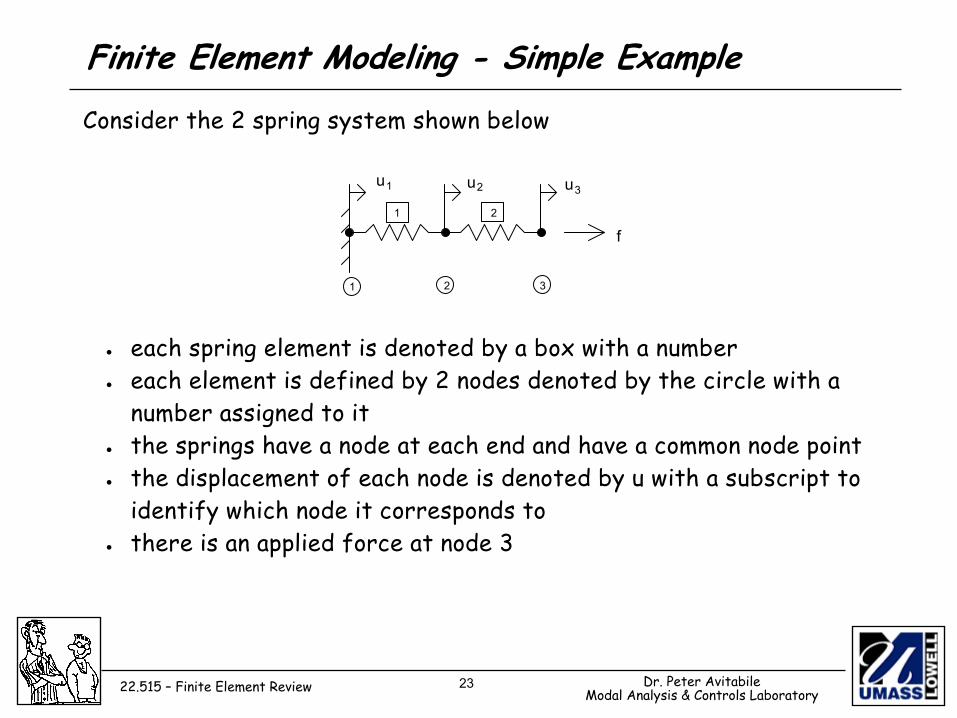
Consider the 2 spring system shown below
• each spring element is denoted by a box with a number • each element is defined by 2 nodes denoted by the circle with a
number assigned to it • the springs have a node at each end and have a common node point • the displacement of each node is denoted by u with a subscript to
identify which node it corresponds to • there is an applied force at node 3
Finite Element Modeling - Simple Example
1 2 3
1 2 f
u 1 u 2 u 3
24 Dr. Peter AvitabileModal Analysis & Controls Laboratory22.515 – Finite Element Review
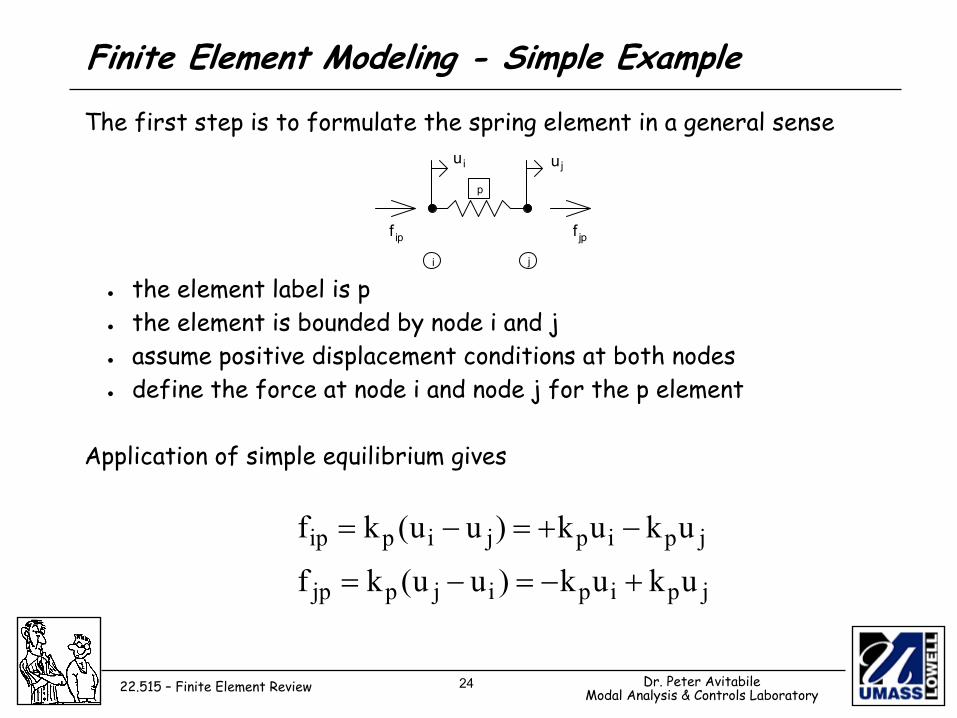
The first step is to formulate the spring element in a general sense
• the element label is p • the element is bounded by node i and j • assume positive displacement conditions at both nodes • define the force at node i and node j for the p element
Application of simple equilibrium gives
Finite Element Modeling - Simple Example
i j
p
f
u i u j
f ip jp
jpipijpjp
jpipjipip
ukuk)uu(kf
ukuk)uu(kf
+−=−=
−+=−=
25 Dr. Peter AvitabileModal Analysis & Controls Laboratory22.515 – Finite Element Review
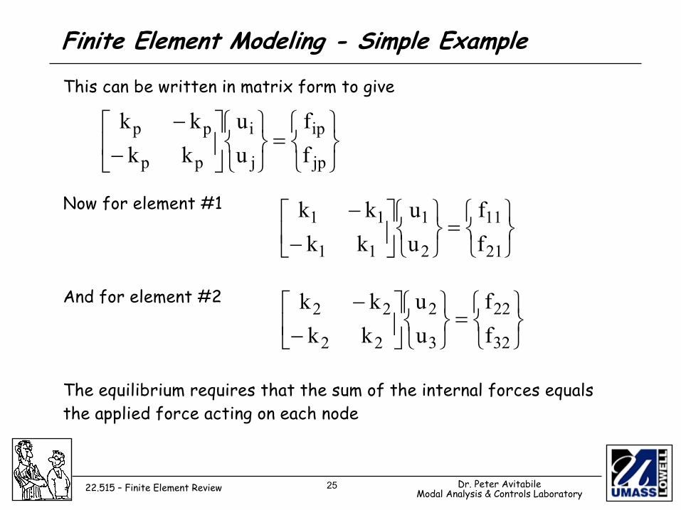
This can be written in matrix form to give
Now for element #1
And for element #2 The equilibrium requires that the sum of the internal forces equals the applied force acting on each node
Finite Element Modeling - Simple Example
=
−
−
jp
ip
j
i
pp
pp
ff
uu
kkkk
=
−
−
21
11
2
1
11
11
ff
uu
kkkk
=
−
−
32
22
3
2
22
22
ff
uu
kkkk
26 Dr. Peter AvitabileModal Analysis & Controls Laboratory22.515 – Finite Element Review
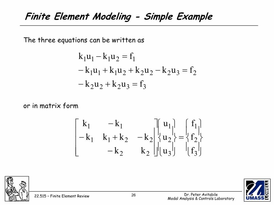
The three equations can be written as
or in matrix form
Finite Element Modeling - Simple Example
33222
232222111
12111
fukukfukukukuk
fukuk
=+−=−++−
=−
=
−−+−
−
3
2
1
3
2
1
22
2211
11
fff
uuu
kkkkkk
kk
27 Dr. Peter AvitabileModal Analysis & Controls Laboratory22.515 – Finite Element Review
Finite Element Modeling - Simple Example
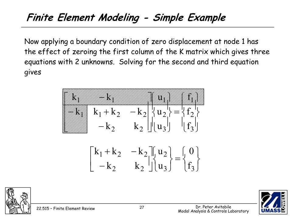
Now applying a boundary condition of zero displacement at node 1 has the effect of zeroing the first column of the K matrix which gives three equations with 2 unknowns. Solving for the second and third equation gives
=
−
−+
33
2
22
221
f0
uu
kkkkk
=
−−+−
−
3
2
1
3
2
1
22
2211
11
fff
uuu
kkkkkk
kk
28 Dr. Peter AvitabileModal Analysis & Controls Laboratory22.515 – Finite Element Review
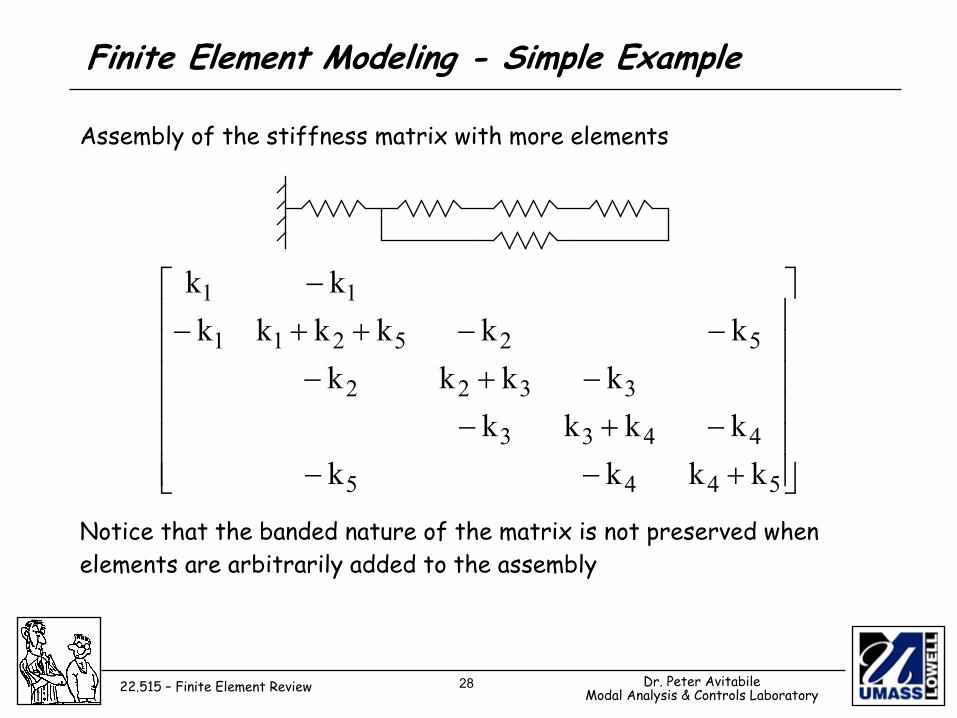
Finite Element Modeling - Simple Example
Assembly of the stiffness matrix with more elements Notice that the banded nature of the matrix is not preserved when elements are arbitrarily added to the assembly
+−−−+−
−+−−−++−
−
5445
4433
3322
525211
11
kkkkkkkk
kkkkkkkkkk
kk
29 Dr. Peter AvitabileModal Analysis & Controls Laboratory22.515 – Finite Element Review
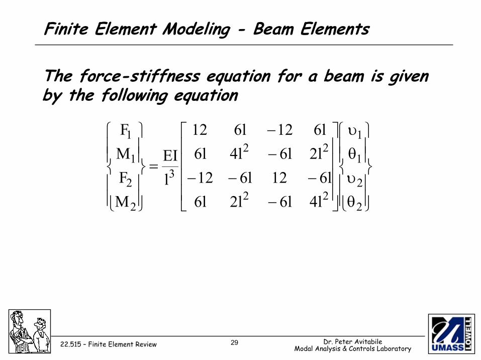
Finite Element Modeling - Beam Elements
The force-stiffness equation for a beam is given by the following equation
θυθυ
−−−−
−−
=
2
2
1
1
22
22
3
2
2
1
1
l4l6l2l6l612l612
l2l6l4l6l612l612
lEI
MFMF
30 Dr. Peter AvitabileModal Analysis & Controls Laboratory22.515 – Finite Element Review
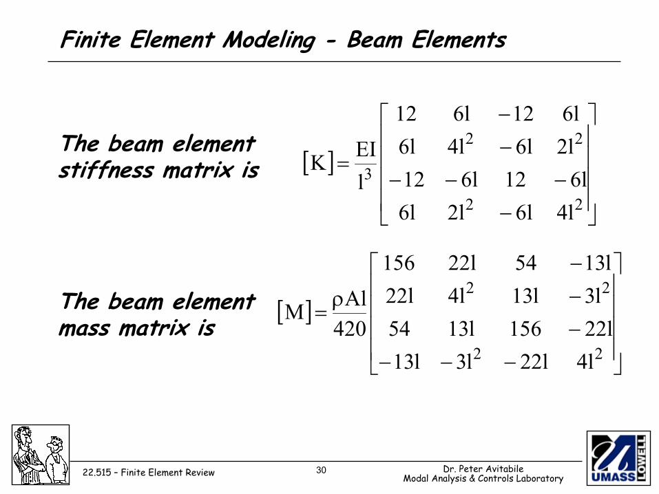
Finite Element Modeling - Beam Elements
The beam element stiffness matrix is
The beam element mass matrix is
[ ]
−−−−
−−
=
22
22
3
l4l6l2l6l612l612
l2l6l4l6l612l612
lEIK
[ ]
−−−−−−
ρ=
22
22
l4l22l3l13l22156l1354
l3l13l4l22l1354l22156
420AlM
31 Dr. Peter AvitabileModal Analysis & Controls Laboratory22.515 – Finite Element Review
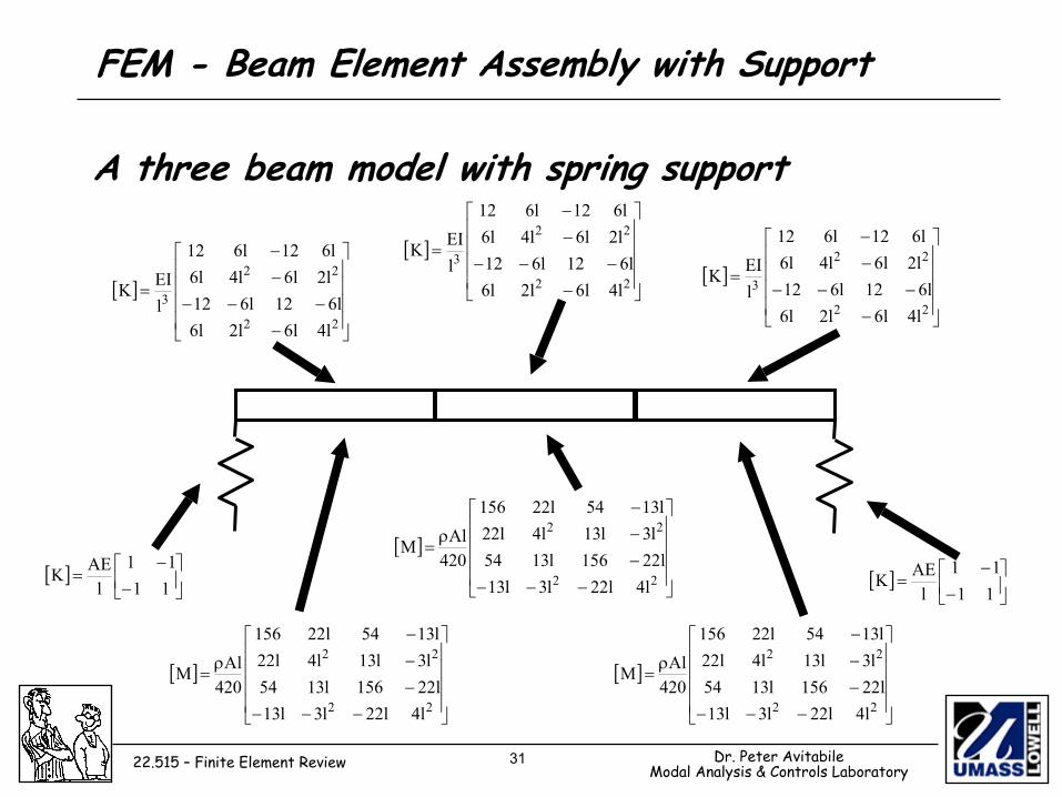
FEM - Beam Element Assembly with Support
A three beam model with spring support
[ ]
−−−−
−−
=
22
22
3
l4l6l2l6l612l612
l2l6l4l6l612l612
lEIK
[ ]
−−−−
−−
=
22
22
3
l4l6l2l6l612l612
l2l6l4l6l612l612
lEIK
[ ]
−−−−
−−
=
22
22
3
l4l6l2l6l612l612
l2l6l4l6l612l612
lEIK
[ ]
−
−=
1111
lAEK [ ]
−
−=
1111
lAEK
[ ]
−−−−−−
ρ=
22
22
l4l22l3l13l22156l1354
l3l13l4l22l1354l22156
420AlM
[ ]
−−−−−−
ρ=
22
22
l4l22l3l13l22156l1354
l3l13l4l22l1354l22156
420AlM [ ]
−−−−−−
ρ=
22
22
l4l22l3l13l22156l1354
l3l13l4l22l1354l22156
420AlM
32 Dr. Peter AvitabileModal Analysis & Controls Laboratory22.515 – Finite Element Review
−−−−
−−
22
22
l4(l6(l2l6l6(12(l612
l2l6l4l6l612l6)12
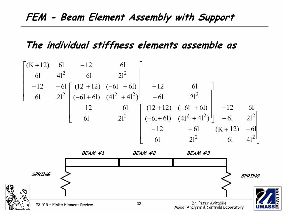
BEAM #1
−−−−
−++−++
22
22
l4l6l2l6l6)12l612
l2l6)l4)l6l612)l6)12
BEAM #3
FEM - Beam Element Assembly with Support
The individual stiffness elements assemble as
−−−−
−++−++
22
22
l4(l6(l2l6l6(12(l612
l2l6)l4)l6l612)l6)12
BEAM #2
+K(
SPRING
+K(
SPRING
33 Dr. Peter AvitabileModal Analysis & Controls Laboratory22.515 – Finite Element Review
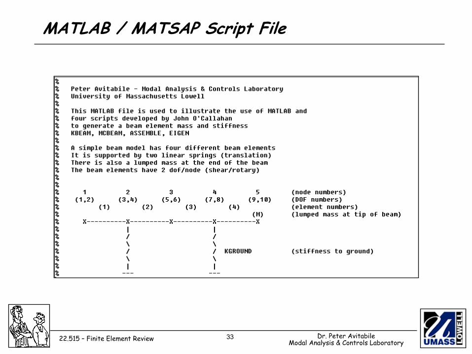
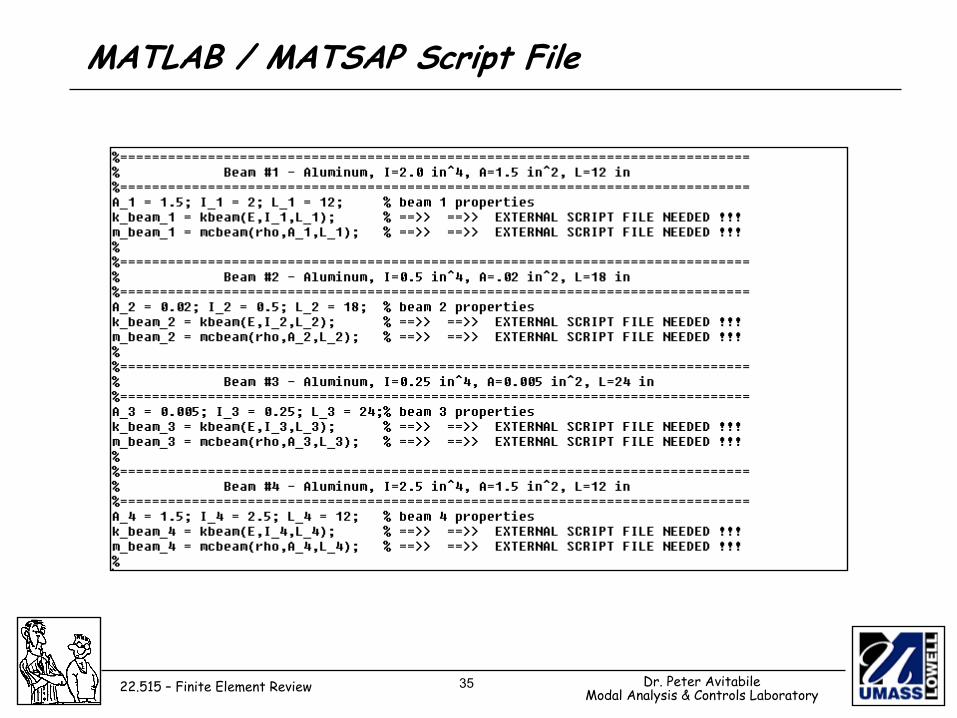
MATLAB / MATSAP Script File
34 Dr. Peter AvitabileModal Analysis & Controls Laboratory22.515 – Finite Element Review
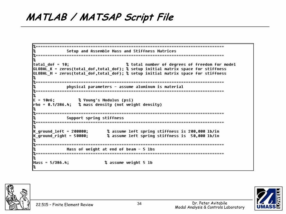
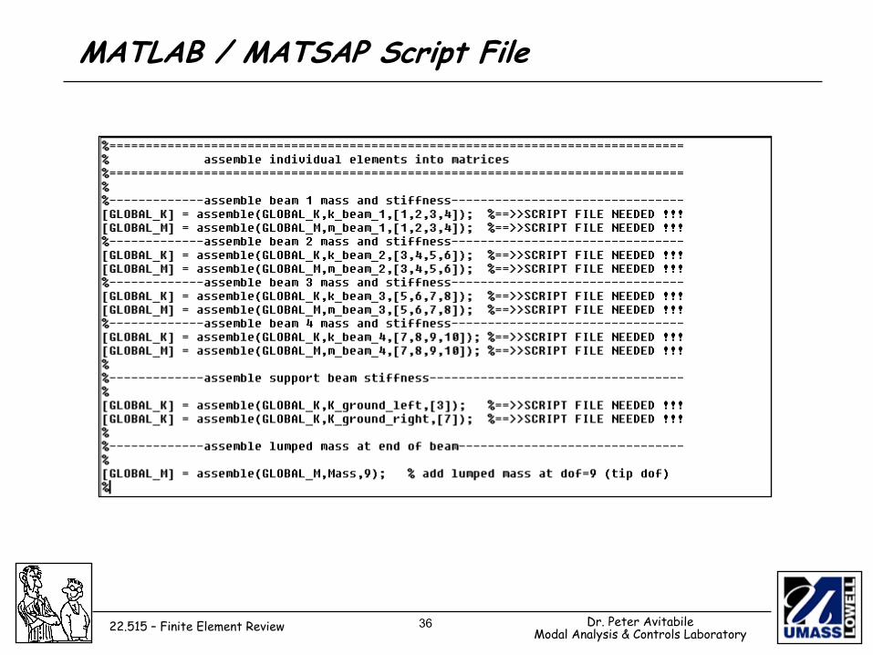
MATLAB / MATSAP Script File
35 Dr. Peter AvitabileModal Analysis & Controls Laboratory22.515 – Finite Element Review
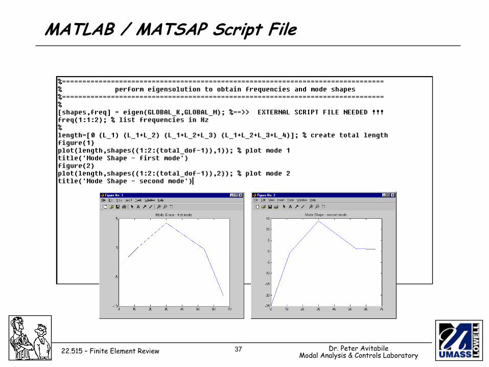
MATLAB / MATSAP Script File
36 Dr. Peter AvitabileModal Analysis & Controls Laboratory22.515 – Finite Element Review
MATLAB / MATSAP Script File
37 Dr. Peter AvitabileModal Analysis & Controls Laboratory22.515 – Finite Element Review
MATLAB / MATSAP Script File
38 Dr. Peter AvitabileModal Analysis & Controls Laboratory22.515 – Finite Element Review
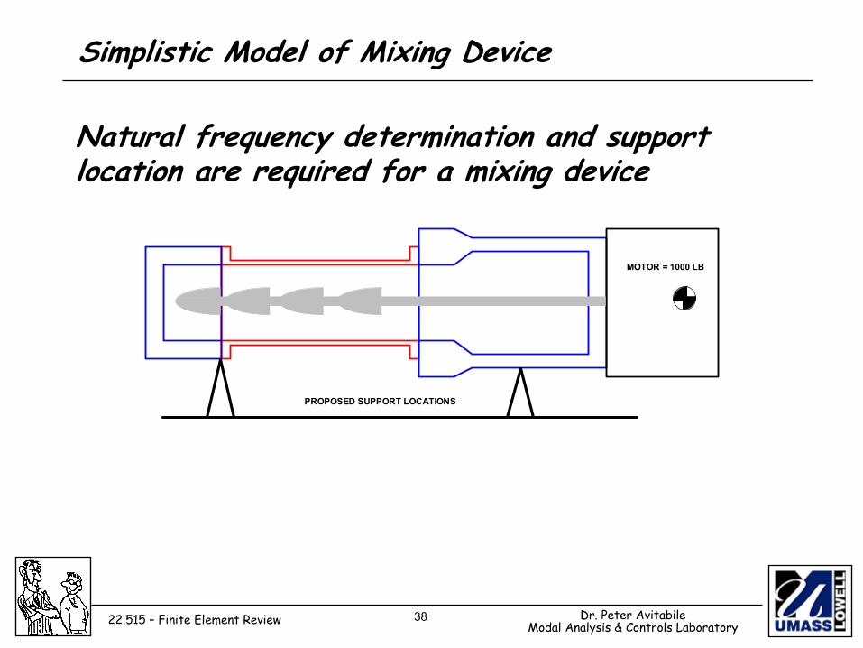
Simplistic Model of Mixing Device
Natural frequency determination and support location are required for a mixing device
MOTOR = 1000 LB
PROPOSED SUPPORT LOCATIONS
39 Dr. Peter AvitabileModal Analysis & Controls Laboratory22.515 – Finite Element Review
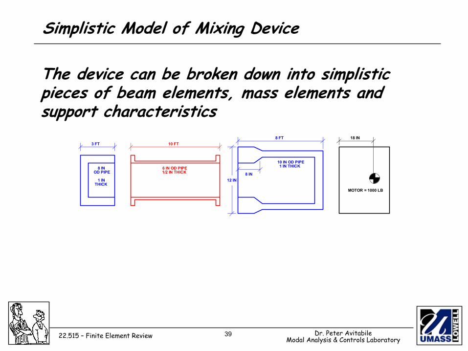
Simplistic Model of Mixing Device
The device can be broken down into simplistic pieces of beam elements, mass elements and support characteristics
MOTOR = 1000 LB
18 IN 8 FT
8 IN 12 IN
10 FT
10 IN OD PIPE 1 IN THICK 6 IN OD PIPE
1/2 IN THICK
3 FT
8 IN
1 IN THICK
OD PIPE
40 Dr. Peter AvitabileModal Analysis & Controls Laboratory22.515 – Finite Element Review
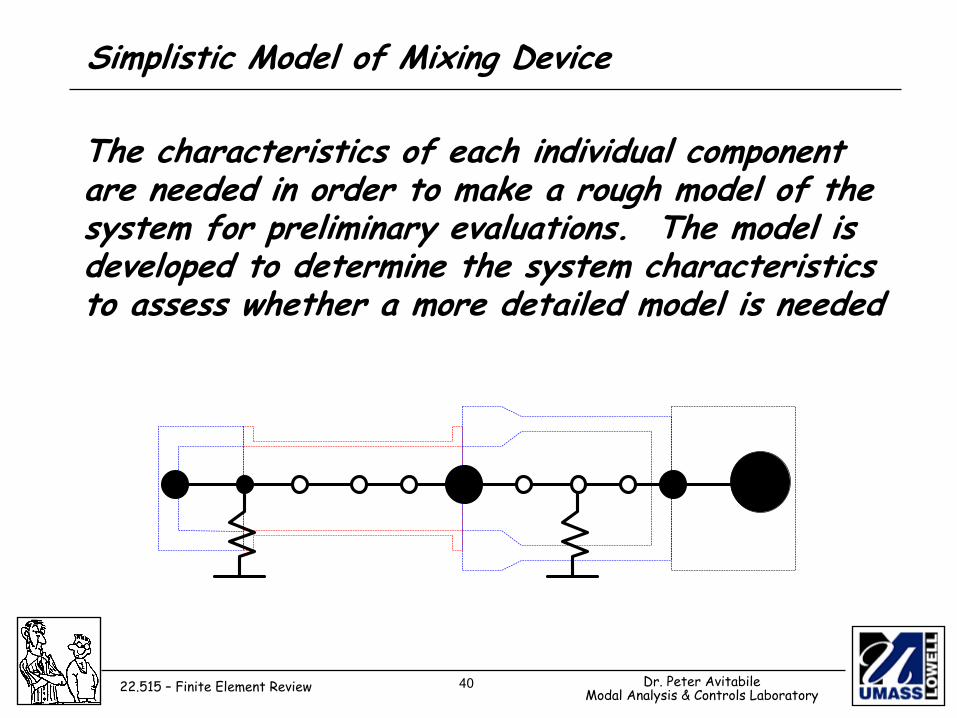
Simplistic Model of Mixing Device
The characteristics of each individual component are needed in order to make a rough model of the system for preliminary evaluations. The model is developed to determine the system characteristics to assess whether a more detailed model is needed
41 Dr. Peter AvitabileModal Analysis & Controls Laboratory22.515 – Finite Element Review
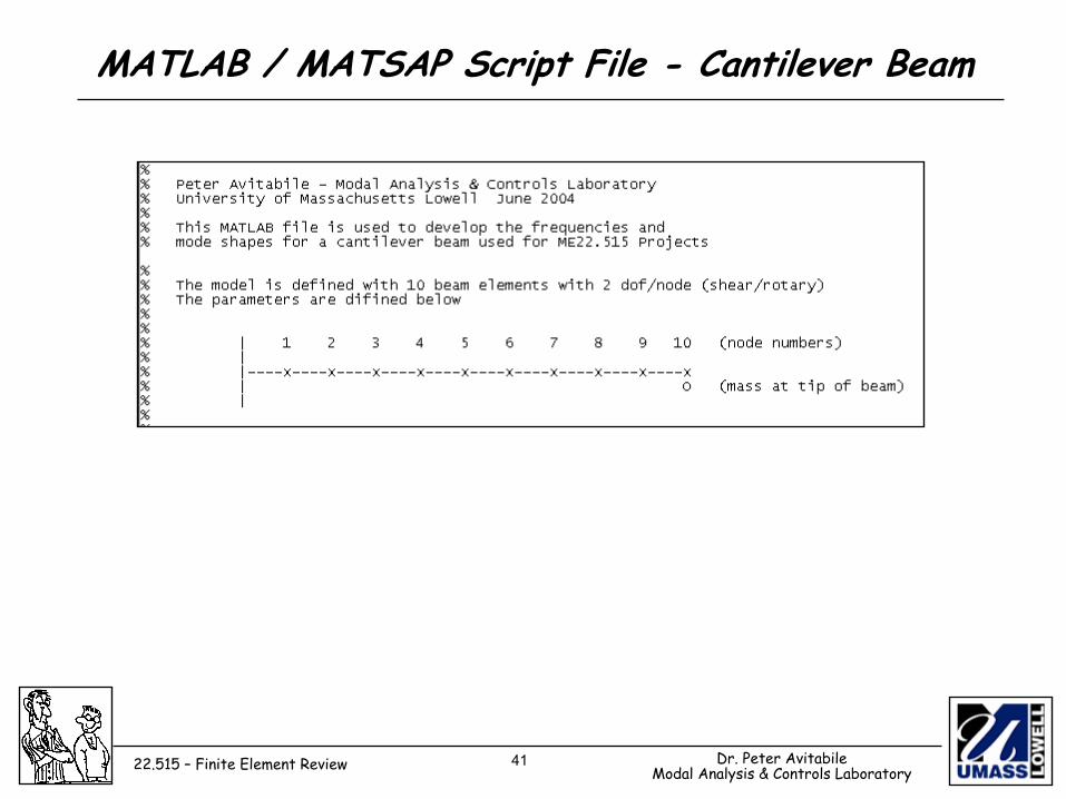
MATLAB / MATSAP Script File - Cantilever Beam
42 Dr. Peter AvitabileModal Analysis & Controls Laboratory22.515 – Finite Element Review
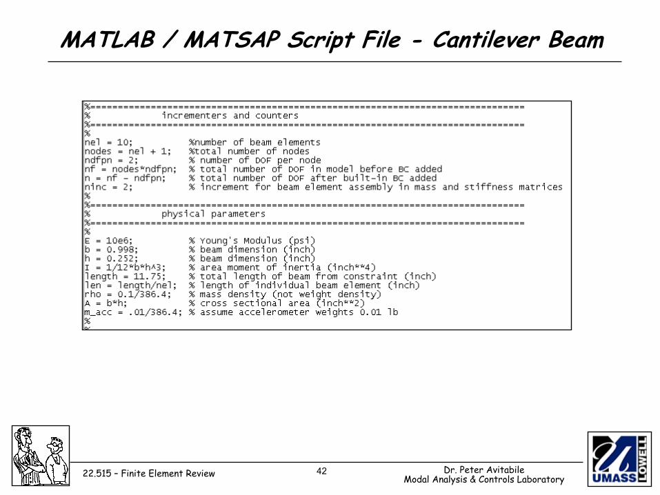
MATLAB / MATSAP Script File - Cantilever Beam
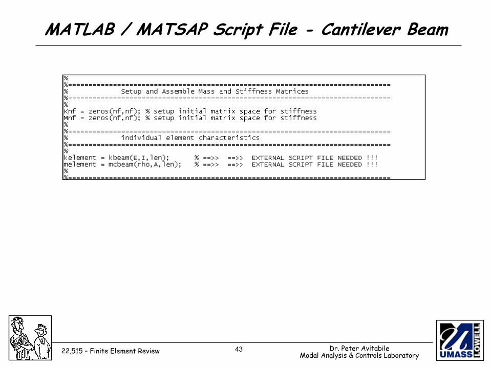
43 Dr. Peter AvitabileModal Analysis & Controls Laboratory22.515 – Finite Element Review
MATLAB / MATSAP Script File - Cantilever Beam
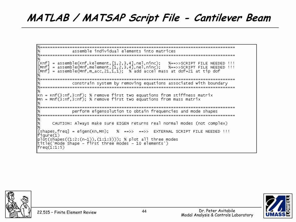
44 Dr. Peter AvitabileModal Analysis & Controls Laboratory22.515 – Finite Element Review
MATLAB / MATSAP Script File - Cantilever Beam