Rethinking CMB Foregrounds: Getting Ready for the Low Signal to...
31
Rethinking CMB Foregrounds: Getting Ready for the Low Signal to Foreground Era Jens Chluba CMB Workshop 2017, UC San Diego La Jolla, Nov 29 th , 2017 -4 -2 0 2 4 0.1 1 10 10 100 1000 10 10 10 10 10 ° ° ° Multipole moment Temperature E-modes Lensing B-modes GW B-modes r=0.05 r=0.001 BK14 SPTPol POLARBEAR 1 3 6 10 30 60 100 300 600 1000 3000 ν [GHz] 10 -1 10 0 10 1 10 2 10 3 10 4 low redshift y-distortion for y = 2 x 10 -6 relativistic correction to y signal Damping signal cooling effect CRR negative branch negative branch PIXIE sensitivity negative branch negative branch Late time absorption JC, Hill and Abitbol, MNRAS, 2017 (ArXiv: 1701.00274)
Transcript of Rethinking CMB Foregrounds: Getting Ready for the Low Signal to...

Rethinking CMB Foregrounds: Getting Ready for the Low Signal to Foreground Era
Jens Chluba CMB Workshop 2017, UC San Diego
La Jolla, Nov 29th, 2017
2.3 Sensitivity forecasts for r 17
-4
-2
0
2
4 0.1110
10 100 1000
10
10
10
10
10°°°
Multipole moment
Angular scale
(+
1)C
/2π
µK2
Temperature
E-modes
Lensing B-modesGW B-modesr=0.05
r=0.001
BK14
SPTPolPOLARBEAR
Figure 6. Theoretical predictions for the temperature (black), E-mode (red), and tensor B-mode (blue)power spectra. Primordial B-mode spectra are shown for two representative values of the tensor-to-scalarratio: r = 0.001 and r = 0.05. The contribution to tensor B modes from scattering at recombination peaksat ` ⇠ 80 and from reionization at ` < 10. Also shown are expected values for the contribution to Bmodes from gravitationally lensed E modes (green). Current measurements of the B-mode spectrum areshown for BICEP2/Keck Array (light orange), POLARBEAR (orange), and SPTPol (dark orange). Thelensing contribution to the B-mode spectrum can be partially removed by measuring the E and exploitingthe non-Gaussian statistics of the lensing.
2.3 Sensitivity forecasts for r
Achieving the CMB-S4 target sensitivity of �(r) ⇠ 10�3 will require exquisite measurements of the B-modepower spectrum. It is expected that CMB-S4 will target the degree-scale recombination feature rather thanthe tens-of-degree-scale reionization feature (see Fig. 6), because these largest scales are di�cult to accessfrom the ground due to atmosphere and sidelobe pickup (though some Stage-3 ground-based experimentsare attempting this measurement, notably CLASS [24]).
As can be seen from Fig. 6, the first requirement for this level of sensitivity to r is a substantial leap forwardin raw instrument sensitivity. For ground-based bolometric detectors, which are individually limited insensitivity by the random arrival of background photons, this means a large increase in detector count. Theforecasts in this section use a baseline of 250,000 detectors operating for four years (or 106 detector years),dedicated solely to maximizing sensitivity to r. It will be necessary to split this total e↵ort among manyelectromagnetic frequencies, to separate the CMB from polarized Galactic foregrounds. The forecasts hereassume eight frequency bands, ranging from 30 to 270 GHz. Contamination from gravitationally lensed Emodes must also be mitigated. While a precise prediction for the cosmological mean of the lensing B-modepower spectrum can be made and subtracted from the observed spectrum, there will be a sample varianceresidual between this prediction and the real lensing B modes on a particular patch of sky. To suppressthis sample variance, it will be necessary to “delens” the B-mode maps with a prediction for the lensing
CMB-S4 Science Book
1 3 6 10 30 60 100 300 600 1000 3000ν [GHz]
10-1
100
101
102
103
104
ΔI
[ Jy
sr-1
]
low redshift y-distortion for y = 2 x 10⁻⁶
relativistic correction to y signalDamping signalcooling effectCRR
negative branch
negative branch
PIXIE sensitivity
negative branch
negative branch
Late timeabsorption
JC, Hill and Abitbol, MNRAS, 2017 (ArXiv: 1701.00274)
The E/B-mode signals that we are after2.3 Sensitivity forecasts for r 17
-4
-2
0
2
4 0.1110
10 100 1000
10
10
10
10
10°°°
Multipole moment
Angular scale(
+1)C
/2π
µK2
Temperature
E-modes
Lensing B-modesGW B-modesr=0.05
r=0.001
BK14
SPTPolPOLARBEAR
Figure 6. Theoretical predictions for the temperature (black), E-mode (red), and tensor B-mode (blue)power spectra. Primordial B-mode spectra are shown for two representative values of the tensor-to-scalarratio: r = 0.001 and r = 0.05. The contribution to tensor B modes from scattering at recombination peaksat ` ⇠ 80 and from reionization at ` < 10. Also shown are expected values for the contribution to Bmodes from gravitationally lensed E modes (green). Current measurements of the B-mode spectrum areshown for BICEP2/Keck Array (light orange), POLARBEAR (orange), and SPTPol (dark orange). Thelensing contribution to the B-mode spectrum can be partially removed by measuring the E and exploitingthe non-Gaussian statistics of the lensing.
2.3 Sensitivity forecasts for r
Achieving the CMB-S4 target sensitivity of �(r) ⇠ 10�3 will require exquisite measurements of the B-modepower spectrum. It is expected that CMB-S4 will target the degree-scale recombination feature rather thanthe tens-of-degree-scale reionization feature (see Fig. 6), because these largest scales are di�cult to accessfrom the ground due to atmosphere and sidelobe pickup (though some Stage-3 ground-based experimentsare attempting this measurement, notably CLASS [24]).
As can be seen from Fig. 6, the first requirement for this level of sensitivity to r is a substantial leap forwardin raw instrument sensitivity. For ground-based bolometric detectors, which are individually limited insensitivity by the random arrival of background photons, this means a large increase in detector count. Theforecasts in this section use a baseline of 250,000 detectors operating for four years (or 106 detector years),dedicated solely to maximizing sensitivity to r. It will be necessary to split this total e↵ort among manyelectromagnetic frequencies, to separate the CMB from polarized Galactic foregrounds. The forecasts hereassume eight frequency bands, ranging from 30 to 270 GHz. Contamination from gravitationally lensed Emodes must also be mitigated. While a precise prediction for the cosmological mean of the lensing B-modepower spectrum can be made and subtracted from the observed spectrum, there will be a sample varianceresidual between this prediction and the real lensing B modes on a particular patch of sky. To suppressthis sample variance, it will be necessary to “delens” the B-mode maps with a prediction for the lensing
CMB-S4 Science Book
de-lensing
lensed E-modes

Average CMB spectral distortions
1 3 6 10 30 60 100 300 600 1000 3000ν [GHz]
10-1
100
101
102
103
104Δ
I [ J
y sr
-1]
low redshift y-distortion for y = 2 x 10⁻⁶
relativistic correction to y signalDamping signalcooling effectCRR
negative branch
negative branch
PIXIE sensitivity
negative branch
negative branch
Late timeabsorption
JC, 2016, MNRAS (ArXiv:1603.02496)

Some of the foregrounds that are in the way…
Planck Collaboration: Di↵use component separation: Foreground maps
Ad
0.01 0.1 1 10mKRJ @ 545 GHz
Fig. 11. Maximum posterior (top) and posterior rms (bottom) thermal dust intensity maps derived from the joint baseline analysisof Planck, WMAP, and 408 MHz observations.
24
Planck Collaboration: Di↵use component separation: Foreground maps
Asd
0.01 0.1 1 10mKRJ @ 30 GHz
Fig. 10. Maximum posterior (top) and posterior rms (bottom) spinning dust intensity maps derived from the joint baseline analysisof Planck, WMAP, and 408 MHz observations. The top panel shows the sum of the two spinning dust components in the base-line model, evaluated at 30 GHz, whereas the bottom shows the standard deviation of only the primary spinning dust component,evaluated at 22.8 GHz.
23
Planck Collaboration: Di↵use component separation: Foreground maps
A�
0 10 100 1000
cm�6pc
Fig. 9. Maximum posterior (top) and posterior rms (bottom) free-free emission measure maps derived from the joint baseline analysisof Planck, WMAP, and 408 MHz observations.
22
Planck Collaboration: Di↵use component separation: Foreground maps
As
10 30 100 300KRJ @ 408 MHz
Fig. 8. Maximum posterior (top) and posterior rms (bottom) synchrotron intensity maps derived from the joint baseline analysis ofPlanck, WMAP, and 408 MHz observations.
21
Thermal dust
Spinning dust
free-free emission
Synchrotron

Future foreground problem for CMB signals
• B-mode and distortion signals are quite small - Low signal to ‘noise’ regime with foregrounds dominating in most bands
- De-lensing required to reach r ~ 10-3 or nT constraint

Future foreground problem for CMB signals
• B-mode and distortion signals are quite small - Low signal to ‘noise’ regime with foregrounds dominating in most bands
- De-lensing required to reach r ~ 10-3 or nT constraint
• Spatially varying foreground signals across the sky - Complex spatial and spectral structure (⟷ non-Gaussian, degeneracies, etc) - Foreground SEDs can depend on many parameters
(e.g., 3 single temperature thermal dust component and AME even more) - Intensity and polarization both need to be dealt with
• Many sensitive channels required to disentangle the different components (probably more than we think…)
• Control of systematics (calibration, beams etc)
• Need to model all the obvious aspects!
• Need to prepare for surprises (redundancies & nulling)!
Include effects of averaging signals
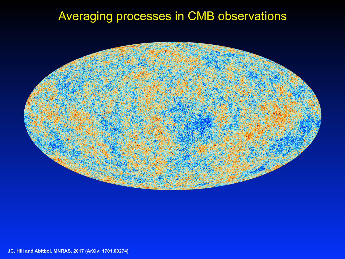
Averaging processes in CMB observations
JC, Hill and Abitbol, MNRAS, 2017 (ArXiv: 1701.00274)

Averaging processes in CMB observations
JC, Hill and Abitbol, MNRAS, 2017 (ArXiv: 1701.00274)
Blackbody SED in every volume element

Averaging processes in CMB observations
JC, Hill and Abitbol, MNRAS, 2017 (ArXiv: 1701.00274)
?
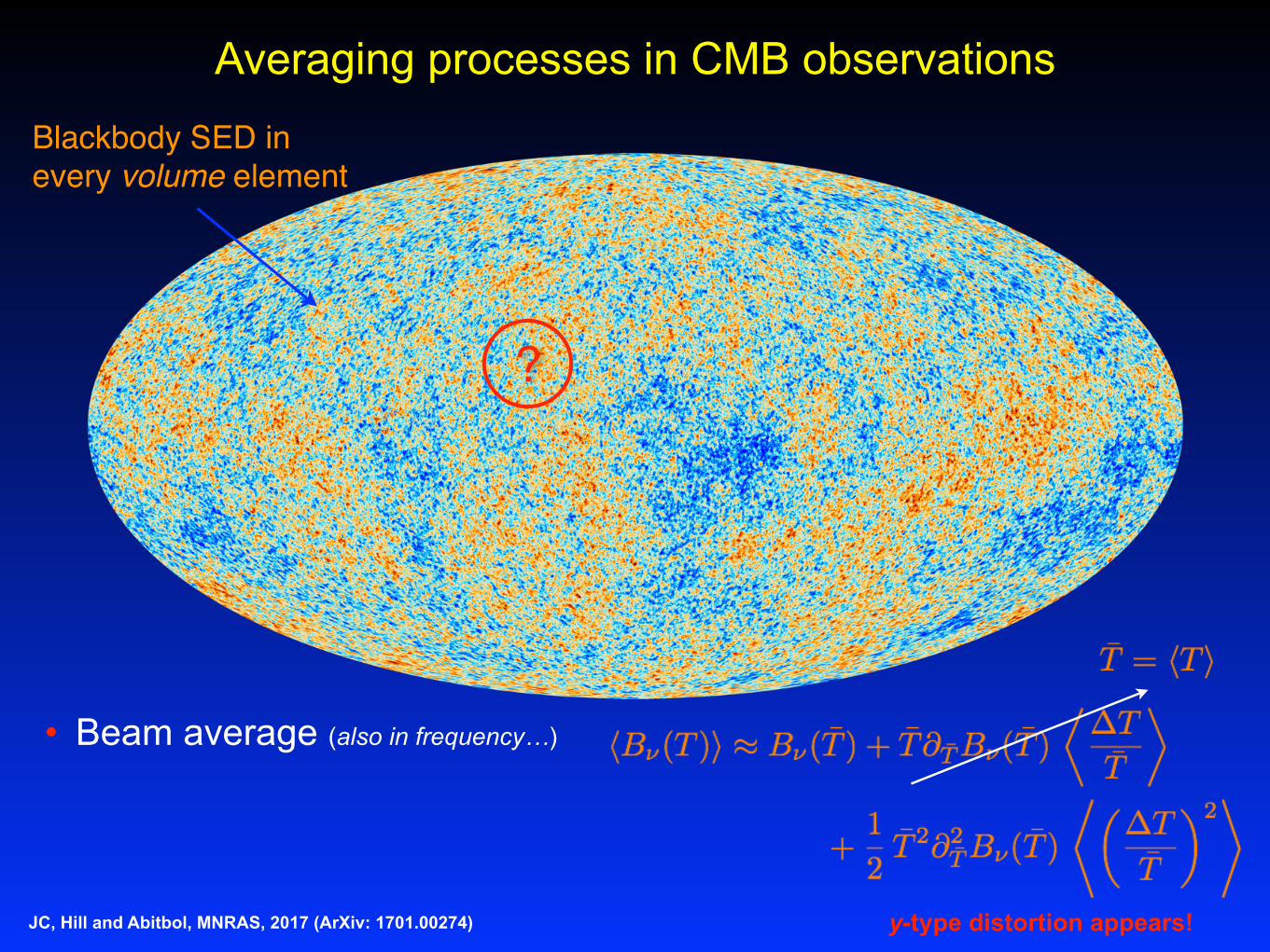
• Beam average (also in frequency…)
Blackbody SED in every volume element

Averaging processes in CMB observations
JC, Hill and Abitbol, MNRAS, 2017 (ArXiv: 1701.00274)
?
• Beam average (also in frequency…)
Blackbody SED in every volume element

Averaging processes in CMB observations
JC, Hill and Abitbol, MNRAS, 2017 (ArXiv: 1701.00274)
?
• Beam average (also in frequency…)
Blackbody SED in every volume element
Averaging processes in CMB observations
JC, Hill and Abitbol, MNRAS, 2017 (ArXiv: 1701.00274)
?
• Beam average (also in frequency…)
y-type distortion appears!
Blackbody SED in every volume element

Averaging processes in CMB observations
JC, Hill and Abitbol, MNRAS, 2017 (ArXiv: 1701.00274)
?
• Beam average (also in frequency…)
?
y-type distortion appears!
Blackbody SED in every volume element
Averaging processes in CMB observations
JC, Hill and Abitbol, MNRAS, 2017 (ArXiv: 1701.00274)
?
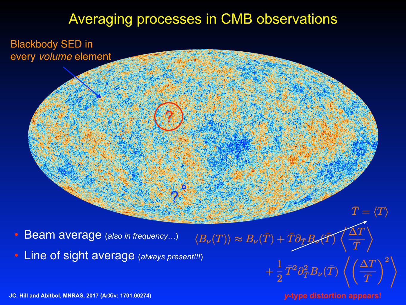
• Beam average (also in frequency…)
?
• Line of sight average (always present!!!)
y-type distortion appears!
Blackbody SED in every volume element

Averaging processes in CMB observations
JC, Hill and Abitbol, MNRAS, 2017 (ArXiv: 1701.00274)
?
• Beam average (also in frequency…)
?
• Line of sight average (always present!!!)
y-type distortion appears!
?x Ylm
Blackbody SED in every volume element
Averaging processes in CMB observations
JC, Hill and Abitbol, MNRAS, 2017 (ArXiv: 1701.00274)
?
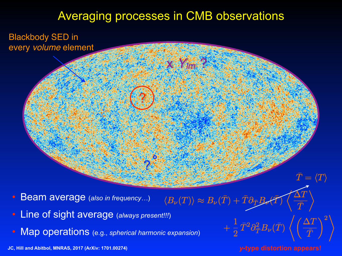
• Beam average (also in frequency…)
?
• Line of sight average (always present!!!)
• Map operations (e.g., spherical harmonic expansion)
y-type distortion appears!
?x Ylm
Blackbody SED in every volume element

Averaging processes in CMB observations
JC, Hill and Abitbol, MNRAS, 2017 (ArXiv: 1701.00274)
?
• Beam average (also in frequency…)
?
• Line of sight average (always present!!!)
• Map operations (e.g., spherical harmonic expansion)
y-type distortion appears!
?x Ylm
Averaging processes change the SED!!!
Blackbody SED in every volume element

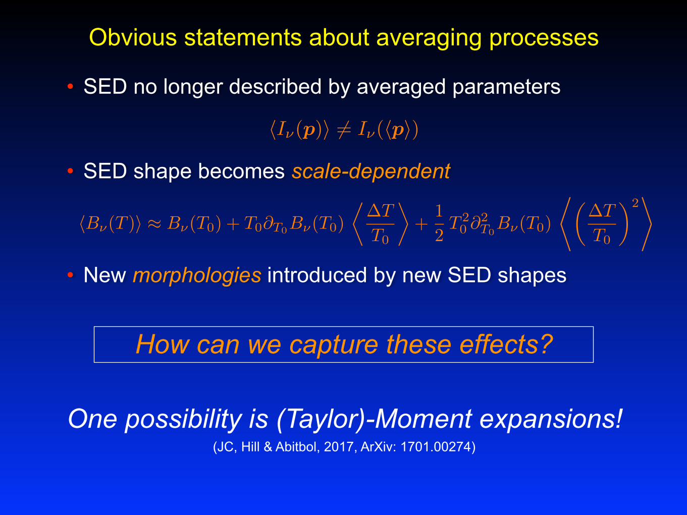
Obvious statements about averaging processes
• SED no longer described by averaged parameters
• SED shape becomes scale-dependent
• New morphologies introduced by new SED shapes
hI⌫(p)i 6= I⌫(hpi)
hB⌫(T )i ⇡ B⌫(T0) + T0@T0B⌫(T0)
⌧�T
T0
�+
1
2T 20 @
2T0B⌫(T0)
*✓�T
T0
◆2+

Obvious statements about averaging processes
• SED no longer described by averaged parameters
• SED shape becomes scale-dependent
• New morphologies introduced by new SED shapes
hI⌫(p)i 6= I⌫(hpi)
How can we capture these effects?
hB⌫(T )i ⇡ B⌫(T0) + T0@T0B⌫(T0)
⌧�T
T0
�+
1
2T 20 @
2T0B⌫(T0)
*✓�T
T0
◆2+
Obvious statements about averaging processes
• SED no longer described by averaged parameters
• SED shape becomes scale-dependent
• New morphologies introduced by new SED shapes
hI⌫(p)i 6= I⌫(hpi)
How can we capture these effects?
One possibility is (Taylor)-Moment expansions! (JC, Hill & Abitbol, 2017, ArXiv: 1701.00274)
hB⌫(T )i ⇡ B⌫(T0) + T0@T0B⌫(T0)
⌧�T
T0
�+
1
2T 20 @
2T0B⌫(T0)
*✓�T
T0
◆2+
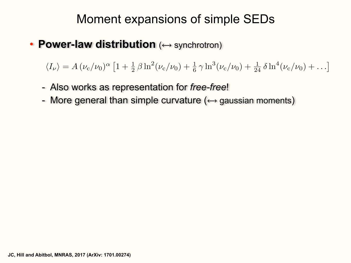
Moment expansions of simple SEDs
JC, Hill and Abitbol, MNRAS, 2017 (ArXiv: 1701.00274)
• Power-law distribution (⟷ synchrotron)
- Also works as representation for free-free! - More general than simple curvature (⟷ gaussian moments)
hI⌫i = A (⌫c/⌫0)↵⇥1 + 1
2 � ln2(⌫c/⌫0) +16 � ln
3(⌫c/⌫0) +124 � ln
4(⌫c/⌫0) + . . .⇤

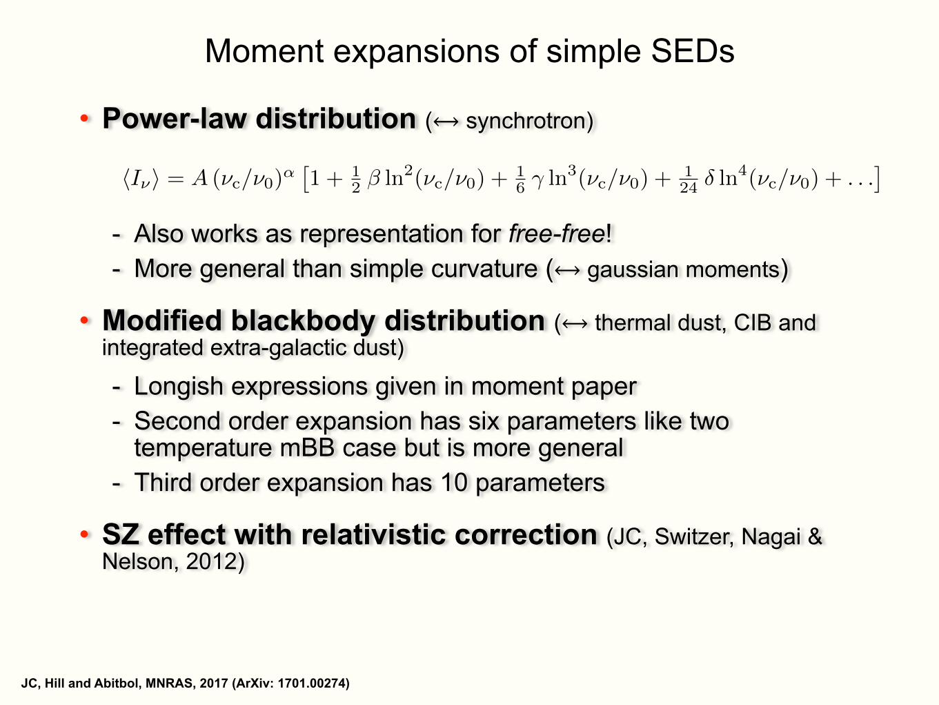
Moment expansions of simple SEDs
JC, Hill and Abitbol, MNRAS, 2017 (ArXiv: 1701.00274)
• Power-law distribution (⟷ synchrotron)
- Also works as representation for free-free! - More general than simple curvature (⟷ gaussian moments)
• Modified blackbody distribution (⟷ thermal dust, CIB and integrated extra-galactic dust) - Longish expressions given in moment paper - Second order expansion has six parameters like two
temperature mBB case but is more general - Third order expansion has 10 parameters
hI⌫i = A (⌫c/⌫0)↵⇥1 + 1
2 � ln2(⌫c/⌫0) +16 � ln
3(⌫c/⌫0) +124 � ln
4(⌫c/⌫0) + . . .⇤
Moment expansions of simple SEDs
JC, Hill and Abitbol, MNRAS, 2017 (ArXiv: 1701.00274)
• Power-law distribution (⟷ synchrotron)
- Also works as representation for free-free! - More general than simple curvature (⟷ gaussian moments)
• Modified blackbody distribution (⟷ thermal dust, CIB and integrated extra-galactic dust) - Longish expressions given in moment paper - Second order expansion has six parameters like two
temperature mBB case but is more general - Third order expansion has 10 parameters
• SZ effect with relativistic correction (JC, Switzer, Nagai & Nelson, 2012)
hI⌫i = A (⌫c/⌫0)↵⇥1 + 1
2 � ln2(⌫c/⌫0) +16 � ln
3(⌫c/⌫0) +124 � ln
4(⌫c/⌫0) + . . .⇤

Moment expansions of simple SEDs
JC, Hill and Abitbol, MNRAS, 2017 (ArXiv: 1701.00274)
• Power-law distribution (⟷ synchrotron)
- Also works as representation for free-free! - More general than simple curvature (⟷ gaussian moments)
• Modified blackbody distribution (⟷ thermal dust, CIB and integrated extra-galactic dust) - Longish expressions given in moment paper - Second order expansion has six parameters like two
temperature mBB case but is more general - Third order expansion has 10 parameters
• SZ effect with relativistic correction (JC, Switzer, Nagai & Nelson, 2012)
• Can be easily generalized to polarization case!!!
hI⌫i = A (⌫c/⌫0)↵⇥1 + 1
2 � ln2(⌫c/⌫0) +16 � ln
3(⌫c/⌫0) +124 � ln
4(⌫c/⌫0) + . . .⇤
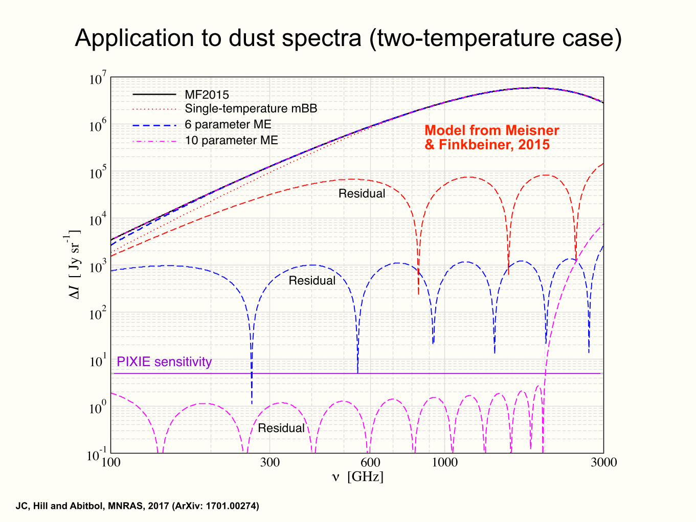
Application to dust spectra (two-temperature case)
JC, Hill and Abitbol, MNRAS, 2017 (ArXiv: 1701.00274)
Rethinking CMB foregrounds 13
commute, we only have to deal with moments of the form !12...2,!13...3,!12...23...3,!2...23...3,!2...2 and!3...3. The relevant spectral func-tions are I1i... j(⌫c, p) = Ii... j(⌫c, p)/A0 with i, j 2 {2, 3} ⌘ {↵, �}, sothat the moments !12...2, !13...3 and !12...23...3 can again be absorbedby defining !d
i...i j... j = !i...i j... j+!1i...i j... j/A0. Assuming narrow bandsand W(�, ⌫) = B(�)F(⌫), we then find
hI⌫i =A0 (⌫/⌫0)↵⌫3
ex � 1
(1 +
12!d
22 ln2(⌫/⌫0)
+!d23 ln(⌫/⌫0) Y1(x) +
12!d
33Y2(x)
+16!d
222 ln3(⌫/⌫0) +12!d
223 ln2(⌫/⌫0)Y1(x)
+12!d
233 ln(⌫/⌫0)Y2(x) +16!d
333Y3(x) + . . .)
↵ =hA0(r)↵(r)i
A0,
1T=hA0(r)/T (r)i
A0(48)
!d2...23...3 =
DA0(r)[(↵(r) � ↵]k [(T/T (r) � 1]m
E
A0.
Higher order terms can be easily added in a similar way. This ex-pression again captures all the degrees of freedom introduced by theaveraging inside the beam and along the line of sight. Note that thesimple product assuming individual superpositions of power-lawand gray-body spectra would be insu�cient, since the cross-terms/ lnk(⌫/⌫0) Ym(x), would not have independent coe�cients to takeinto account possible correlations between ↵ and T . For example,the term for k = 1 and m = 1 would be absent.
6.1 Behavior in the Rayleigh-Jeans limit
In the Rayleigh-Jeans limit (h⌫ ⌧ kT ), we can re-express the mod-ified blackbody spectrum as
IRJ⌫ (A0,↵,T ) ⇡ A0 (⌫/⌫0)↵+2
"1 �
x2+
x2
12�
x4
720+ . . .
#. (49)
This represents a superposition of power-law spectra, which inprinciple can be approximated with Eq. (21). Since x = h⌫/kT ,the temperature variations of the dust itself enter as a weight-factorfor the power-law moment amplitudes, introducing specific corre-lations among the moments. The Taylor series of 1/(ex
� 1) fur-thermore can only be recovered when allowing di↵erences betweenpower-laws instead of just sums as considered previously. We willdiscuss the applicability of this approximation below (Sect. 6.3.1).
6.2 Alternative parameterizations and weighting schemes
In Sect. 5.2.1, we illustrated how the choice of parameters andweighting a↵ects the moment expansion for gray-body spectra. Inparticular, we found that the recovered best-fitting parameters fortruncated moment expansions are sensitive to these choices. In asimilar manner as for the gray-body spectra, by setting ⌫0 = kT/hand rewriting I⌫(A0,↵,T ) = A0 (⌫/⌫0)↵ ⌫3/(eh⌫/kT
� 1) as
I⌫ = A0
kTh
!3 x3+↵
ex � 1= B(T,↵)
x3+↵⇣T/T
⌘3+↵
ex T/T � 1(50)
we can derive an alternative moment expansion for the modifiedblackbody spectra with new weighting B(T,↵) = A0 (kT/h)3+↵.However, we find that this approach does not significantly changethe capabilities of the moment expansion to represent di↵erentSEDs. It only leads to a re-summation of terms up to a given mo-ment order. We therefore did not consider this approach any further.
100 300 600 1000 3000ν [GHz]
10-1
100
101
102
103
104
105
106
107ΔI
[ Jy
sr-1
]MF2015Single-temperature mBB6 parameter ME10 parameter ME
PIXIE sensitivity
Residual
Residual
Residual
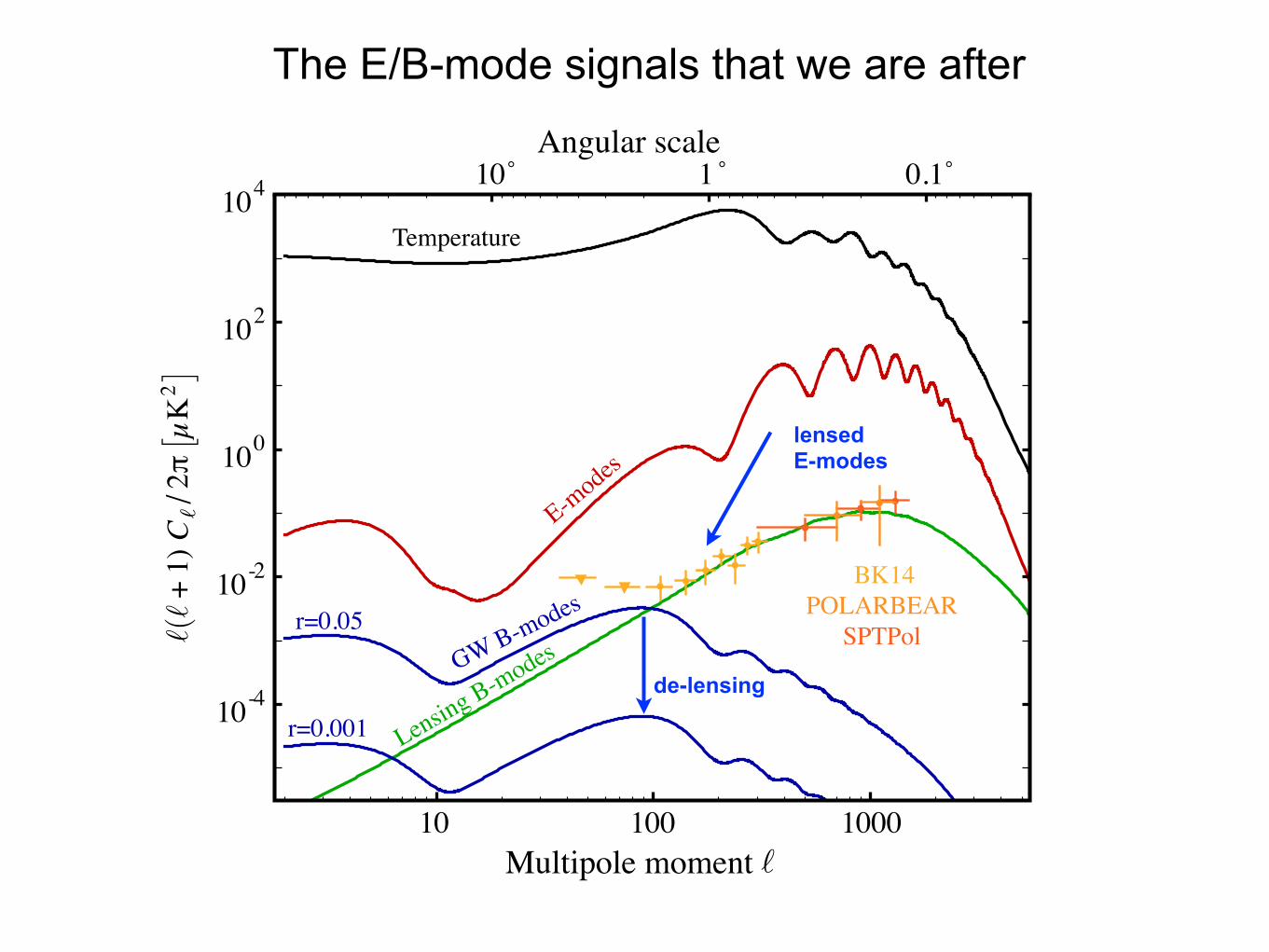
Figure 6. Representation of a two-temperature modified blackbody spec-trum from Meisner & Finkbeiner (2015) using a varying number of mo-ments (see text for details). The long-dashed lines show the residuals incomparison with the estimated absolute sensitivity of PIXIE.
6.3 Two-temperature dust models
To illustrate the application of the moment expansion, let us con-sider a simple two-temperature dust model, with SED parame-ters p = {A1, A2,↵1,↵2,T1,T2}. We then have A = A1 + A2,↵ = (A1↵1 + A2↵2)/A, T = A/(A1/T1 + A2/T2) and the moments
!d2...23...3 =
2X
a=1
Aa
A(↵a � ↵)k(T/Ta � 1)m. (51)
The general behavior of the moment expansion for di↵erent casesis similar to that of gray-body spectra, as mentioned above. Theadditional parameter, ↵, causes the number of moments per pertur-bation order to increase strongly. For example, adding all secondorder moment terms means 3 extra parameters instead of 1 for thegray-body spectrum; at third order we need 7 instead of 2 and soon. The required number of parameters can thus grow quickly forcomplicated dust distribution functions.
To illustrate the method, let us consider a concrete example,setting the model parameters to P1 = {A1, A2,↵1,↵2,T1,T2} =
{A f1, A (1 � f1), 1.63, 2.82, 9.75 K, 15.7 K} with f1 = 0.34188 and⌫0 = 3 THz, based on recent modeling of CMB data (Meisner& Finkbeiner 2015). We fix A such that hI⌫i ' 3388 Jy sr�1 at⌫ = 100 GHz, but for illustrations of the method, the absolute valuedoes not matter, as the spectral shape is fixed without the amplitude.We assume 200 frequency bins in log-⌫ of di↵erent ranges and per-form a simple �2-fit using Eq. (50) setting ⌫0 = kT/h. This choiceof the pivot frequency leads to faster convergence. Representing theresultant spectrum (see Fig. 6) with a single-temperature modifiedblackbody in the range 100 GHz . ⌫ . 3 THz yields ↵ = 1.819 andT = 18.45 K. We find that at low frequencies this approximationshows a large departure from the true SED, underestimating theemission by a factor of two (see Fig. 6). Adding the first order mo-ment corrections, we find ↵ = 1.270, T = 15.27 K, !d
22 = �0.4438,!d
23 = 0.1695 and !d33 = 0.2094, which provides an approxima-
tion that is better than ' 0.4% at 300 GHz . ⌫ . 3 THz, departingonly notably at low frequencies, reaching ' 20% at ⌫ ' 100 GHz(see Fig. 6). This representation uses the same number of parame-ters (six in total) as the input model, but without assuming a two-temperature case, and can in principle already capture a broaderrange of distributions in temperature and spectral indices.
c� 0000 RAS, MNRAS 000, 000–000
Model from Meisner & Finkbeiner, 2015
Application to dust spectra (blind)
JC, Hill and Abitbol, MNRAS, 2017 (ArXiv: 1701.00274)
14 Chluba et al.
The convergence of the moment representation also dependson the frequency range that is assumed in the fitting process. For asecond order moment representation at 100 GHz . ⌫ . 2 THz, weobtain ↵ = 1.412, T = 14.84 K, !d
22 = �0.2793, !d23 = 0.05132
and !d33 = 0.2191. This representation improves the fit at low fre-
quencies, with the departure decreasing to . 8% at ⌫ ' 100 GHz.This illustrates that in precision measurements over a wide rangeof frequencies, the high frequency part of the dust spectrum candrive the solution away from the optimal solution at low frequen-cies. This could a↵ect the ability to recover primordial distortionsignals in high precision CMB spectroscopy, but also is relevantto the modeling of foregrounds for primordial B-modes. Incorrectand incomplete (truncated) parameterizations for the foregroundscan thus yield biased results. Convergence properties of the mo-ment expansion can again be tested by varying the moment order,which provides a powerful diagnostic, but is limited by the avail-able number of channels.
If we now include all moments up to third order (3+3+4=10parameters), we find ↵ = 2.057, T = 13.33 K, !d
22 = 0.002363,!d
23 = �0.4189, !d33 = 0.3789, !d
222 = �0.004326, !d223 = 0.5326,
!d233 = �0.2657 and !d
333 = 0.08050 at 100 GHz . ⌫ . 2 THz.We find that this approximation represents the dust spectrum at100 GHz . ⌫ . 2 THz to better than ' 0.06% precision (see Fig. 6).We can see that the higher order moments start decreasing rapidly,showing that the chosen example is in the perturbative regime andconverges fairly quickly. The achieved level of precision would beabout 4 � 5 times better than the expected sensitivity of PIXIE forabsolute CMB spectroscopy (�I⌫ ' 5 Jy/sr; Kogut et al. 2011).Again, the parameterization is more general than simply assuminga two-temperature model, capturing more general distributions oftemperature and spectral indices.
The overall representation of the average spectrum with thethird order moment expansion degrades significantly (by more thanone order of magnitude in terms of absolute precision) when in-creasing the upper frequency to ⌫ = 3 THz. As expected from ourdiscussion of gray-body spectra, in this case higher order momentsare required to compensate for the asymptotic behavior of the basisfunctions. For a given finite order and distribution of temperatures,this behavior is inevitable with the moment expansion. In this case,alternative approaches that directly assume representations of thetemperature distribution functions could be used; however, a pre-cise description of the underlying probability distribution functions(with a significant number of parameters) is still required. Simi-larly, one could use two hierarchies of moment expansions, form-ing a two-temperature basis to improve the local convergence. Weleave a more detailed discussion of these ideas to future work.
6.3.1 Rayleigh-Jeans approximation
We saw in Sect. 6.1, at low frequencies the superposition of dustspectra can be thought of as a superposition of power-laws. It turnsout that using a simple power-law expansion to represent the aver-age dust spectrum for the model discussed above works quite wellat 30 GHz . ⌫ . 500 GHz, when including only N ' 4 moments(6 parameters in total). A sum of synchrotron and dust spectra, rel-evant to CMB applications, also works well with N ' 6 moments(8 parameters in total, which is one less than the input model) at30 GHz . ⌫ . 200 GHz. However, at higher frequencies correc-tions related to the Taylor series of 1/(ex
� 1) become too large sothat many power-law moments (N � 6) have to be included fora su�cient representation of the dust spectrum. In this case, thegeneral dust moment expansion should be preferred.
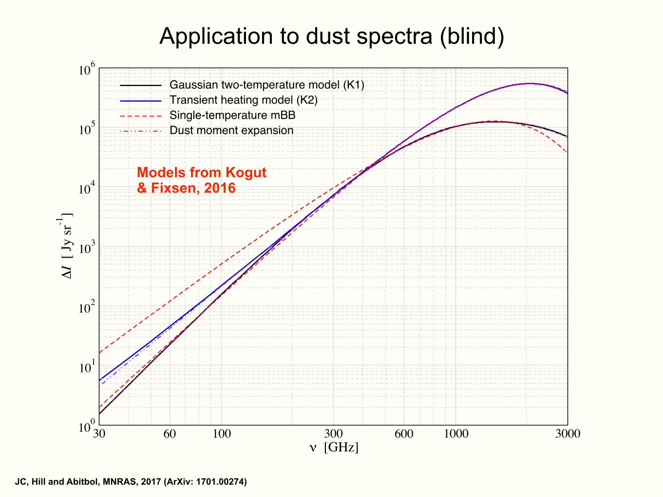
30 60 100 300 600 1000 3000ν [GHz]
100
101
102
103
104
105
106ΔI
[ Jy
sr-1
]Gaussian two-temperature model (K1)Transient heating model (K2)Single-temperature mBBDust moment expansion
Figure 7. Moment representation of dust models recently discussed byKogut & Fixsen (2016). The fits were obtained in the frequency range100 GHz . ⌫ . 2 THz. The red lines assume a single-temperature dustmodel. The violet (double-dotted dashed) lines assume a 10/6 parametermoment expansion for K1/K2. Notice that the 10 parameter moment ex-pansion for K1 covers the input model curve even outside the fit domain.
6.4 Distributions of temperatures
To demonstrate the potential of the dust moment representation,we analyze two more general dust models considered by Kogut &Fixsen (2016), one assuming a sum of two Gaussians for the dusttemperature (K1), the other using a transient heating model12 (K2).The resultant SEDs are shown in Fig. 7.
Without knowing the details of the temperature model, we canrepresent these spectra using the dust moment expansion, Eq. (50).Fitting in the range 100 GHz . ⌫ . 2 THz, we find ↵ = 0.9379 andT = 18.15 K (K1) and ↵ = 1.671 and T = 21.69 K (K2) assum-ing a single-temperature modified blackbody spectrum. The overallamplitude, A0, is be determined using I⌫ = 156.61 Jy/sr (K1) andI⌫ = 220.11 Jy/sr (K2) at ⌫ = 100 GHz. Clearly, this representationfails to approximate the SED for model K1 but already provides agood approximation for K2 (see Fig. 7).
A second order moment expansion (6 parameters) signifi-cantly improves the fit in both cases, leaving residuals at the levelof |�I⌫| . 50 � 200 Jy/sr (K1) and |�I⌫| . 5 Jy/sr (K2) in the con-sidered frequency range. For K2, the 6 parameter moment expan-sion is shown in Fig. 7. We find that at 100 GHz . ⌫ . 2 THz,the transient heating model can be fully represented down to thePIXIE sensitivity using only 6 parameters without a priori assump-tions about the temperature model, while outside this range higherorder moments are required. We also find that for both models, atwo-temperature dust model leads to a similar performance, albeitbeing less general.
Using a third order moment representation (10 parameters),we obtain residuals that are more than one order of magnitudebelow the sensitivity of PIXIE in both cases. For K1, we have↵ = 2.327, T = 14.56 K, !d
22 = �0.2983, !d23 = �0.1718,
!d33 = �0.1396, !d
222 = 0.03299, !d223 = 0.5685, !d
233 = �0.07951and !d
333 = 0.03106 (see Fig. 7). This shows that the dust momentexpansion is able to handle more complicated dust spectra with fewa priori assumptions about the underlying distribution functions.
12 We cordially thank Alan Kogut for providing the average SEDs to us.
c� 0000 RAS, MNRAS 000, 000–000
Models from Kogut & Fixsen, 2016
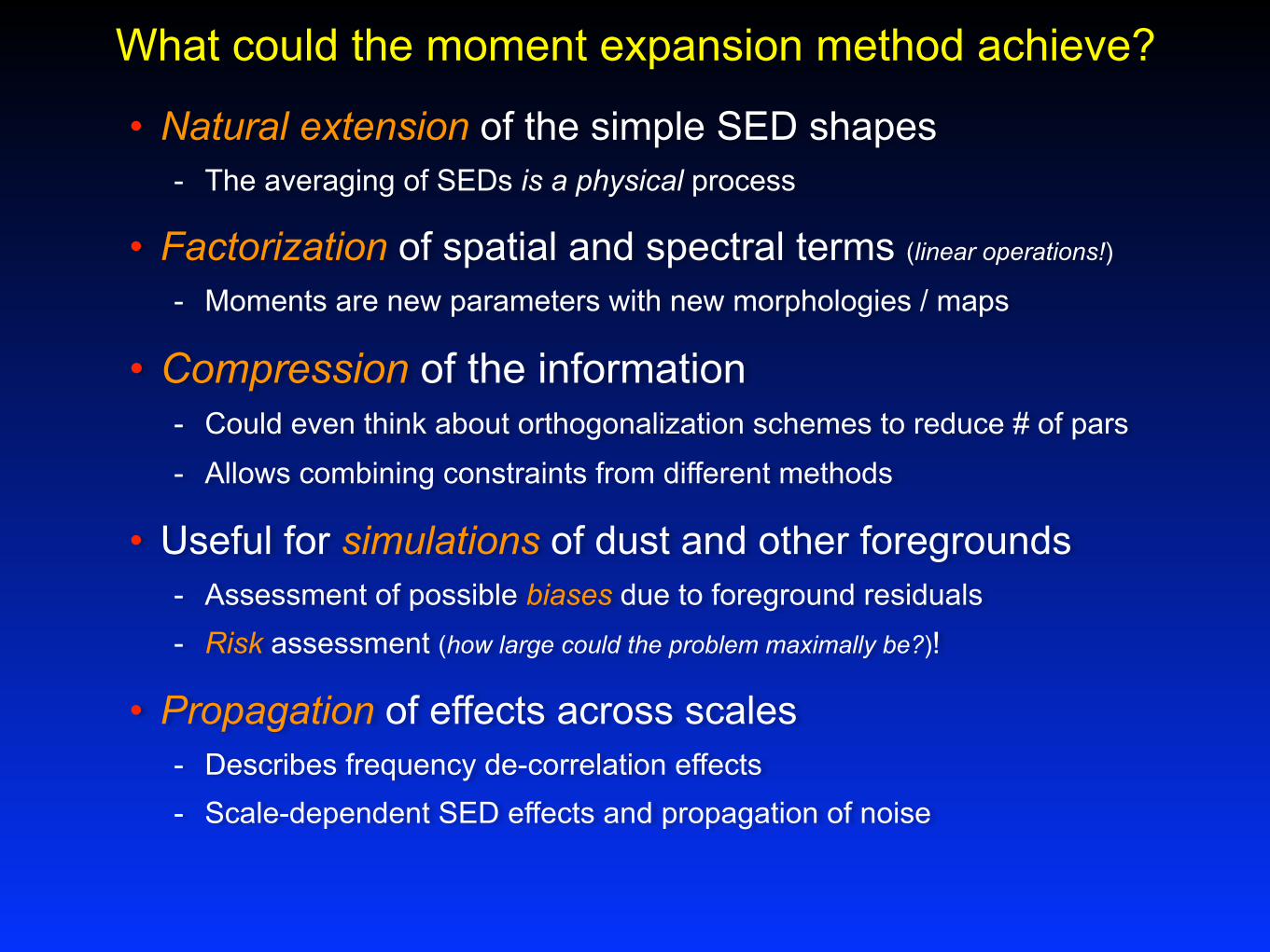
What could the moment expansion method achieve?
• Natural extension of the simple SED shapes - The averaging of SEDs is a physical process
• Factorization of spatial and spectral terms (linear operations!) - Moments are new parameters with new morphologies / maps
• Compression of the information - Could even think about orthogonalization schemes to reduce # of pars
- Allows combining constraints from different methods
• Useful for simulations of dust and other foregrounds - Assessment of possible biases due to foreground residuals - Risk assessment (how large could the problem maximally be?)!
• Propagation of effects across scales - Describes frequency de-correlation effects - Scale-dependent SED effects and propagation of noise
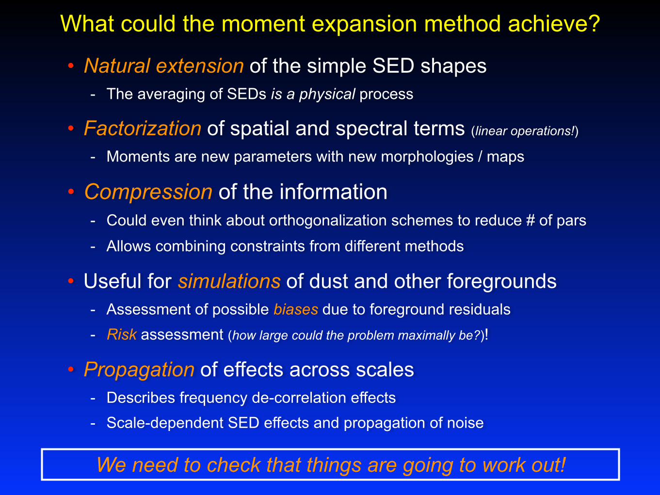
We need to check that things are going to work out!


![What can the CMB tell about cosmic reheating? · WHAT CAN THE CMB TELL ABOUT COSMIC REHEATING? Marco Drewes TU München based on JCAP 1603 (2016) no.03, 013 arXiv:1511.03280 [astro-ph.CO]](https://static.fdocument.org/doc/165x107/5e91deab5155e47de71b91a5/what-can-the-cmb-tell-about-cosmic-reheating-what-can-the-cmb-tell-about-cosmic.jpg)