
Report of laboratory and in-situ validation of micro...
72
20 14 Laurent Spinelle Michel Gerboles Manuel Aleixandre Ozone micro-sensor, αSense, model B4-O3 sensor Report of laboratory and in-situ validation of micro-sensor for monitoring ambient air Report EUR 26681 EN
Transcript of Report of laboratory and in-situ validation of micro...
20 1 4
Laurent Spinelle Michel Gerboles Manuel Aleixandre
Ozone micro-sensor, αSense, model B4-O3 sensor
Report of laboratory and in-situ validation of micro-sensor for monitoring ambient air
Report EUR 26681 EN

European Commission
Joint Research Centre
Institute for Environment and Sustainability
Contact information
Michel Gerboles
Address: Joint Research Centre, Via Enrico Fermi 2749, TP 101, 21027 Ispra (VA), Italy
E-mail: [email protected]
Tel.: +39 0332 78 5652
Fax: +39 0332 78 9931
http://www.jrc.ec.europa.eu/
Legal Notice
This publication is a Technical Report by the Joint Research Centre, the European Commission’s in-house science
service.
It aims to provide evidence-based scientific support to the European policy-making process. The scientific output
expressed does not imply a policy position of the European Commission. Neither the European Commission nor any
person acting on behalf of the Commission is responsible for the use which might be made of this publication.
JRC90463
EUR 26681 EN
ISBN 978-92-79-38538-4 (PDF)
ISSN 1831-9424 (online)
doi:10.2788/84725
Luxembourg: Publications Office of the European Union, 2014
© European Union, 2014
Reproduction is authorised provided the source is acknowledged.
Printed in Italy

SUMMARY
The aim of this report is to evaluate O3-B4 sensors of αSense (UK) with laboratory and field tests under ambient air conditions corresponding to a specific micro-environment: background station, rural areas. The report presents the evaluation of the performances and determination of the laboratory measurement uncertainty, compared to uncertainties fixed by the Data Quality Objective (DQO) of the European Air Quality Directive for indicative methods.
This sensor was found by laboratory experiments to be highly linear and precise with little long term drift up to about 200 days of experiments. In fact good sensitivity and stability of the sensor were observed. However, the scattering of the sensor response at 0 nmol/mol is a drawback if it is planned to monitor low level of O3 (<10 nmol/mol).
Among NO2, NO, CO, CO2, NH3 and SO2, only NO2 was found a significant gaseous interfering compound for this sensor. When monitoring the sole O3, a shortcoming of the sensor was its sensitivity to NO2 that without correction may prevent from correctly estimating O3 when high levels of NO2 and O3 are simultaneously present. However, it is unlikely that NO2 is abundant in rural areas. Humidity had a huge hysteresis effect on the sensor response that was difficult to correct.
The sensor appeared to be slightly influenced by wind velocity, hysteresis, temperature and matrix effect. Conversely, change in pressure, power supply (220 V) did not have an effect on the sensor response likely because of the quality of the DC transformer used in laboratory.
With the laboratory experiments, simple models were established to compute O3 using the sensors responses, NO2 and water vapour or both temperature and relative humidity.
The sensor measurement uncertainty, calculated using the results of all laboratory experiments could meet the Data Quality Objective (30 % of relative expanded uncertainty) provided that these models were applied. Without applying these models, the contribution of humidity and NO2 was found too high.
The sensors, used in field, were calibrated in laboratory at the end of the field exposure of about 4 months. Unfortunately, the field experiments were not successful and valid measurements could not be obtained. Therefore, the models established with the laboratory experiments could not be verified in field.
Further to this study, the application of the sensor as indicative method for O3 fixed measurement at background site/rural areas is not fully validated, a field confirmation of the laboratory results is missing.

4
ENV01- MACPoll
Metrology for Chemical Pollutants in
Air
Laboratory and in-situ validation of Ozone micro-
sensors, αSense, model B4 O3 sensors
Deliverable number: (4.3.5)
Version: 2.0 (comments of manufacturer added)
Date: April 2014
Task 4.3: Testing protocol, procedures and testing of performances of sensors
(JRC, MIKES, INRIM, REG-Researcher (CSIC))

5
JRC
JRC building 44 TP442
via E. Fermi 21027 - Ispra (VA)
Italy
Manuel Aleixandre (REG) - CSIC
Instituto de Física Aplicada,
Serrano 144 - 28006 Madrid
Spain
Reviewed by:
Dr. John Safell (αSense)
MACPoll Collaborator
Acknowledgment:
The authors wish to acknowledge the
collaboration of F. Lagler, N. R. Jensen and A.
Dell’Acqua, our JRC colleagues, for carrying out
air pollution measurements.
The contribution of F. Bonavitacola of Phoenix
Sistemi & Automazione s.a.g.l. (CH) for
developing data acquisition systems is also
granted.

6
1. TASK 4.3: TESTING PROTOCOL, PROCEDURES AND TESTING OF PERFORMANCES
OF SENSORS (JRC, MIKES, INRIM, REG-RESEARCHER (CSIC )) .............................................. 8
1.1 “LABORATORY AND IN-SITU VALIDATION OF MICRO-SENSORS” AND “REPORT OF THE LABORATORY AND IN-
SITU VALIDATION OF MICRO-SENSORS (AND UNCERTAINTY ESTIMATION) AND EVALUATION OF SUITABILITY OF MODEL
EQUATIONS” ..................................................................................................................................................... 9
1.2 TIME SCHEDULE AND ACTIVITIES ............................................................................................................. 9
1.3 PROTOCOL OF EVALUATION .................................................................................................................. 10
1.4 GAS SENSOR TESTED WITHIN MACPOLL ............................................................................................... 11
2 SENSOR IDENTIFICATION ................................................................................................... 12
2.1 MANUFACTURER AND SUPPLIER:........................................................................................................... 12
2.2 SENSOR MODEL AND PART NUMBER: ..................................................................................................... 12
2.3 DATA PROCESSING OF THE SENSOR ...................................................................................................... 12
2.4 AUXILIARY SYSTEMS SUCH AS POWER SUPPLY, TEST BOARD AND DATA ACQUISITION SYSTEM. ................. 12
2.5 PROTECTION BOX AND/OR SENSOR HOLDER USED ................................................................................. 13
3 SCOPE OF VALIDATION ............................... ....................................................................... 14
4 LITERATURE REVIEW: ................................ ......................................................................... 16
5 LABORATORY EXPERIMENTS ............................ ................................................................ 17
5.1 EXPOSURE CHAMBER FOR TEST IN LABORATORY ................................................................................... 17
5.2 GAS MIXTURE GENERATION SYSTEM ..................................................................................................... 19
5.3 REFERENCE METHODS OF MEASUREMENTS ........................................................................................... 19
5.3.1 Methods ..................................................................................................................................... 19
5.3.2 Quality control ............................................................................................................................ 20
5.3.3 Homogeneity .............................................................................................................................. 20
6 METROLOGICAL PARAMETERS ........................... .............................................................. 20
6.1 RESPONSE TIME .................................................................................................................................. 20
6.2 PRE CALIBRATION ................................................................................................................................ 22
6.3 SHORT AND LONG TERM DRIFTS, SHOT TERM REPEATABILITY .................................................................. 23
6.3.1 Repeatability .............................................................................................................................. 23
6.3.2 Short term drift ........................................................................................................................... 24
6.3.3 Long term drift ............................................................................................................................ 26
7 INTERFERENCE TESTING ................................................................................................... 28
7.1 GASEOUS INTERFERING COMPOUNDS ................................................................................................... 28
7.1.1 Nitrogen dioxide - NO2 ............................................................................................................... 30
7.1.2 Nitrogen monoxide - NO ............................................................................................................ 31
7.1.3 Carbon monoxide interference................................................................................................... 31
7.1.4 Carbon dioxide interference ....................................................................................................... 32
7
7.1.5 Sulfur dioxide interference ......................................................................................................... 32
7.1.6 Ammonia interference ................................................................................................................ 33
7.2 AIR MATRIX ......................................................................................................................................... 34
7.3 HYSTERESIS ........................................................................................................................................ 37
7.4 METEOROLOGICAL PARAMETERS .......................................................................................................... 38
7.4.1 Temperature and humidity ......................................................................................................... 38
7.4.2 Wind velocity effect .................................................................................................................... 41
7.5 EFFECT OF CHANGE OF AMBIENT PRESSURE ......................................................................................... 43
7.6 EFFECT OF CHANGE IN POWER SUPPLY ................................................................................................. 44
7.7 CHOICE OF TESTED INTERFERING PARAMETERS IN FULL FACTORIAL DESIGN ............................................ 44
8 LABORATORY MODEL AND UNCERTAINTY .................. ................................................... 45
8.1 EXPERIMENTAL DESIGN ........................................................................................................................ 45
8.2 EXPLORATION OF THE DATA SET ........................................................................................................... 45
8.3 RESULTS ............................................................................................................................................. 46
8.4 UNCERTAINTY ESTIMATION ................................................................................................................... 49
9 FIELD EXPERIMENTS........................................................................................................... 51
9.1 MONITORING STATIONS ........................................................................................................................ 51
9.2 SENSOR EQUIPMENT ............................................................................................................................ 52
9.3 CHECK OF THE SENSOR IN LABORATORY ............................................................................................... 53
9.4 FIELD RESULTS ................................................................................................................................... 54
9.5 ESTIMATION OF FIELD UNCERTAINTY AND CALIBRATION PROCEDURE ....................................................... 56
10 CONCLUSION .................................................................................................................... 56
11 APPENDIX A: DATA SHEET OF ΑSENSE 4-ELECTRODE O3-B4 AND INDIVIDUAL
SENSOR BOARD (ISB) ISSUE 4, 085-2217 USER MANUAL IS SUE 2 ...................................... 58
4 CORRECTING THE DATA USING A SPREADSHEET ........................................................................................ 63
12 APPENDIX B: RESPONSE TIME STEPS.................... ....................................................... 66
13 APPENDIX C: DESIGN OF EXPERIMENTS ................. ..................................................... 69

8
1. Task 4.3: Testing protocol, procedures and testi ng of performances of sensors (JRC, MIKES, INRIM, REG-Researcher (CSIC))
The aim of this task was to validate NO2 and O3 cheap sensors under laboratory. Based on the recommendations of the review (Task 4.1), the graphene sensors and a limited number of sensor types and air pollutants were chosen. At the beginning of the validation a testing protocol was drafted, which was improved and refined during the process of validation experience. This task provided the information needed for estimating the measurement uncertainty of the tested sensors. Further, procedures for the calibration of sensors able to ensure full traceability of measurements of sensors to SI units were also drafted.
The laboratory work package endeavoured to find a solution to the current problem of validation of sensors. In general, the validation of sensors is either carried out in a laboratory using synthetic mixtures, or at an ambient air monitoring station with real ambient matrix. Generally, these results are not reproducible at other sites than the one used during validation. In fact, sensors are highly sensitive to matrix effects, meteorological conditions and gaseous interferences that change from site to site.
Commonly, the validation generally performed by sensor users consists in establishing the minimum parameter set of sensors to describe their selectivity, sensitivity and stability. Since, this features is generally not reproducible from site to site, it was proposed in this project to extend the validation procedure by establishing simplified model descriptions of the phenomena involved in the sensor detection process. Both laboratory experiment in exposure chambers and fine tuning of these models during field experiments were carried out in this project.
The sensors were exposed to controlled atmospheres of gaseous mixtures in exposure chambers. These laboratory controlled atmospheres consisted of a set of mixtures with several levels of NO2/O3 concentrations, under different conditions of temperature and relative humidity and including the main gaseous interfering compounds.
Description of work:
- The tested sensors were selected by CSIC and JRC. The development of the protocol for the evaluation of sensors was carried out by CSIC and JRC. INRIM and MIKES carried out the initial laboratory evaluations of the new NO2 graphene sensors. JRC carried out the experimental test of the selected O3 and NO2 commercial sensors and JRC and the REG-Researcher (CSIC) performed the evaluation of their test results. After laboratory tests, the commercial O3 and NO2 sensors were tested at field sites under real conditions by JRC.
- Along the different step of the project, the protocol for evaluation of sensors was improved by CSIC and JRC based on the test results and the technical feasibility of the experiments.
- The controlled atmospheres of the INRIM and MIKES tests were designed to evaluate the linearity of graphene sensors at different NO2 levels (5) and their stability with respect to temperature (3 levels) and/or relative humidity (3 levels) at constant NO2 level.
- JRC performed laboratory tests to determine the parameters of the NO2 and O3 model equations (task 4.1) using full or partial experimental design of influencing variables (identified in task 4.1). In any case, the controlled atmosphere included at least 5 levels of air pollutants, 3 levels of air pollutants and 3 levels of relative humidity and 2 levels of the chemical interference evidenced in task 4.1.
- CSIC and JRC applied the protocol of evaluation to the commercial sensors with determination of their metrological characteristics: detection limits, response time, poisoning points, hysteresis, etc., measurement uncertainty in laboratory and field experiment.
Activity summary: (The text with yellow background shows the activity reported in this report)
1. Selection of suitable sensors for validation (at least 2 commercially available NO2 sensors, 3 commercially available O3 sensors and the INRIM and MIKES graphene sensors (JRC, REG-Researcher (CSIC))
2. Development of a validation protocol and procedures for calibration of micro-sensors (CSIC)
3. Laboratory evaluation of the INRIM and MIKES graphene sensors: lab tests of NO2 level, temperature, humidity, response time and hysteresis (INRIM)
9
4. Laboratory evaluation of the INRIM and MIKES graphene sensors (lab tests of NO2 concentration, response time, warming time and temperature or humidity effect) (MIKES)
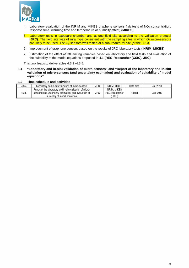
5. Laboratory tests in exposure chamber and at one field site according to the validation protocol (JRC). The field site was of rural type consistent with the sampling sites in which O3 micro-sensors are likely to be used. The O3 sensors was tested at a suburban/rural site (at the JRC).
6. Improvement of graphene sensors based on the results of JRC laboratory tests (INRIM, MIKES)
7. Estimation of the effect of influencing variables based on laboratory and field tests and evaluation of the suitability of the model equations proposed in 4.1 (REG-Researcher (CSIC), JRC)
This task leads to deliverables 4.3.1 -4.3.5.
1.1 “Laboratory and in-situ validation of micro-sensors ” and “Report of the laboratory and in-situ validation of micro-sensors (and uncertainty estima tion) and evaluation of suitability of model equations”
1.2 Time schedule and activities 4.3.4 Laboratory and in-situ validation of micro-sensors JRC INRIM, MIKES Data sets Jul. 2013
4.3.5 Report of the laboratory and in-situ validation of micro-sensors (and uncertainty estimation) and evaluation of
suitability of model equations JRC
INRIM, MIKES, REG-Researcher
(CSIC) Report Dec. 2013
10
1.3 Protocol of evaluation
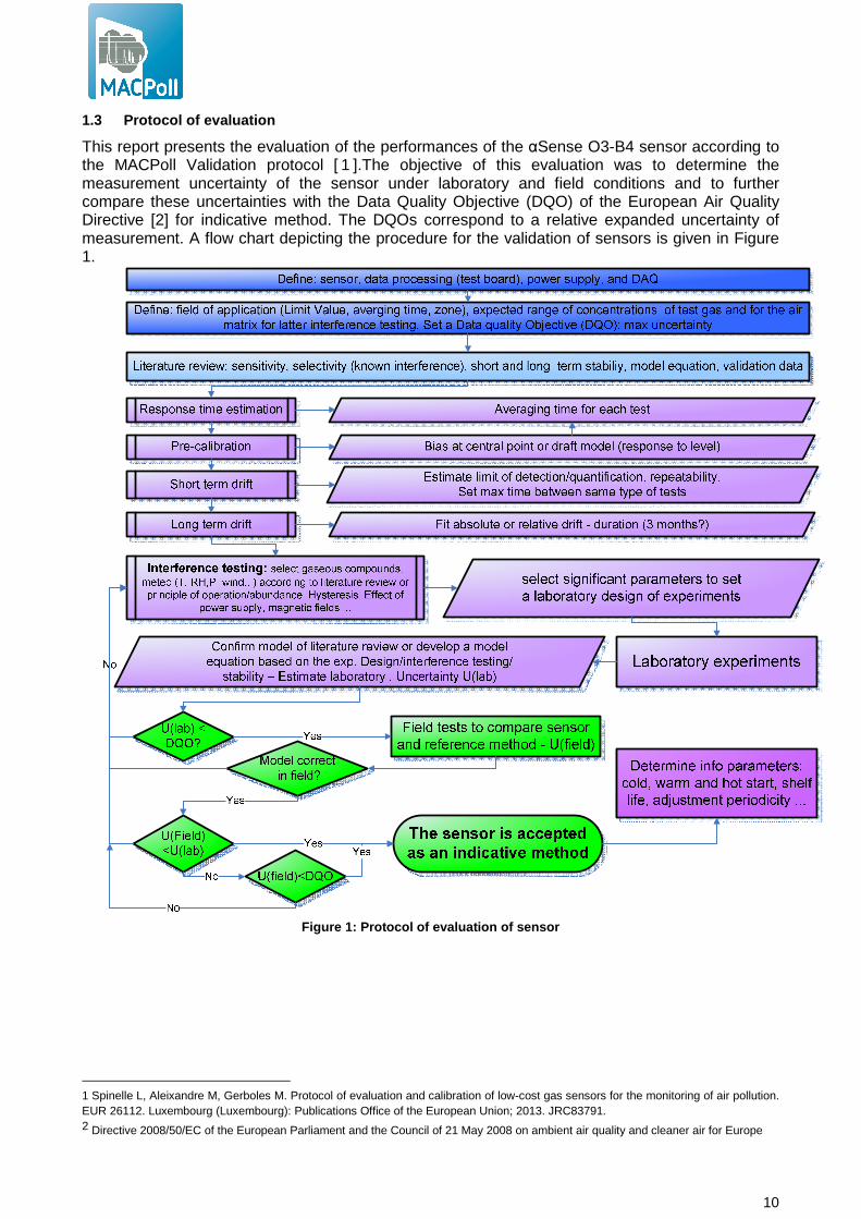
This report presents the evaluation of the performances of the αSense O3-B4 sensor according to the MACPoll Validation protocol [ 1 ].The objective of this evaluation was to determine the measurement uncertainty of the sensor under laboratory and field conditions and to further compare these uncertainties with the Data Quality Objective (DQO) of the European Air Quality Directive [2] for indicative method. The DQOs correspond to a relative expanded uncertainty of measurement. A flow chart depicting the procedure for the validation of sensors is given in Figure 1.
Figure 1: Protocol of evaluation of sensor
1 Spinelle L, Aleixandre M, Gerboles M. Protocol of evaluation and calibration of low-cost gas sensors for the monitoring of air pollution. EUR 26112. Luxembourg (Luxembourg): Publications Office of the European Union; 2013. JRC83791. 2 Directive 2008/50/EC of the European Parliament and the Council of 21 May 2008 on ambient air quality and cleaner air for Europe
11
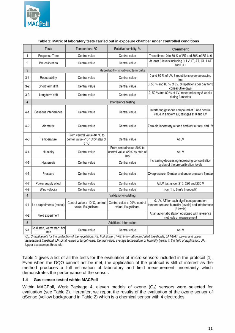
Table 1 gives a list of all the tests for the evaluation of micro-sensors included in the protocol [1]. Even when the DQO cannot not be met, the application of the protocol is still of interest as the method produces a full estimation of laboratory and field measurement uncertainty which demonstrates the performance of the sensor.
1.4 Gas sensor tested within MACPoll
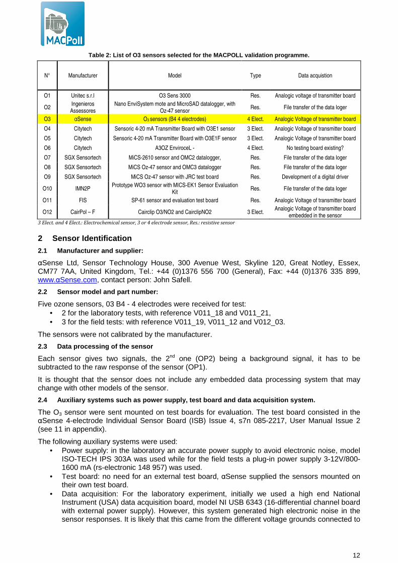
Within MACPoll, Work Package 4, eleven models of ozone (O3) sensors were selected for evaluation (see Table 2). Hereafter, we report the results of the evaluation of the ozone sensor of αSense (yellow background in Table 2) which is a chemical sensor with 4 electrodes.
Table 1: Matrix of laboratory tests carried out in exposure chamber under controlled conditions
Tests Temperature, ºC Relative humidity, % Comment
1 Response Time Central value Central value Three times: 0 to 80 % of FS and 80% of FS to 0
2 Pre-calibration Central value Central value At least 3 levels including 0, LV, IT, AT, CL, LAT
and UAT
3 Repeatability, short-long term drifts
3-1 Repeatability Central value Central value 0 and 80 % of LV, 3 repetitions every averaging
time
3-2 Short term drift Central value Central value 0, 50 % and 80 % of LV, 3 repetitions per day for 3
consecutive days
3-3 Long term drift Central value Central value 0, 50 % and 80 % of LV, repeated every 2 weeks
during 3 months
4 Interference testing
4-1 Gaseous interference Central value Central value Interfering gaseous compound at 0 and central
value in ambient air, test gas at 0 and LV
4-2 Air matrix Central value Central value Zero air, laboratory air and ambient air at 0 and LV
4-3 Temperature From central value-10 °C to
center value +10 °C by step of 5 °C
Central value At LV
4-4 Humidity Central value From central value-20% to
central value +20% by step of 10%
At LV
4-5 Hysteresis Central value Central value Increasing-decreasing-increasing concentration
cycles of the pre-calibration levels
4-6 Pressure Central value Central value Overpressure 10 mbar and under pressure 5 mbar
4-7 Power supply effect Central value Central value At LV test under 210, 220 and 230 V
4-8 Wind velocity Central value Central value from 1 to 5 m/s (needed?)
4 Validation/modelling
4-1 Lab experiments (model) Central value ± 10°C, central
value, if significant Central value ±-20%, central
value, if significant
0, LV, AT for each significant parameter: temperature and humidity (levels) and interference
(2 levels)
4-2 Field experiment At an automatic station equipped with reference
methods of measurement
5 Additional information
5-1 Cold start, warm start, hot
start Central value Central value At LV
CL: Critical levels for the protection of the vegetation, FS: Full Scale, IT/AT: Information and alert thresholds, LAT/UAT: Lower and upper assessment threshold, LV: Limit values or target value, Central value: average temperature or humidity typical in the field of application, UA: Upper assessment threshold
12
Table 2: List of O3 sensors selected for the MACPOLL validation programme.
N° Manufacturer Model Type Data acquistion
O1 Unitec s.r.l O3 Sens 3000 Res. Analogic voltage of transmitter board
O2 Ingenieros Assessores
Nano EnviSystem mote and MicroSAD datalogger, with Oz-47 sensor
Res. File transfer of the data loger
O3 αSense O3 sensors (B4 4 electrodes) 4 Elect. Analogic Voltage of transmitter board
O4 Citytech Sensoric 4-20 mA Transmitter Board with O3E1 sensor 3 Elect. Analogic Voltage of transmitter board
O5 Citytech Sensoric 4-20 mA Transmitter Board with O3E1F sensor 3 Elect. Analogic Voltage of transmitter board
O6 Citytech A3OZ EnviroceL - 4 Elect. No testing board existing?
O7 SGX Sensortech MiCS-2610 sensor and OMC2 datalogger, Res. File transfer of the data loger
O8 SGX Sensortech MiCS Oz-47 sensor and OMC3 datalogger Res. File transfer of the data loger
O9 SGX Sensortech MiCS Oz-47 sensor with JRC test board Res. Development of a digital driver
O10 IMN2P Prototype WO3 sensor with MICS-EK1 Sensor Evaluation
Kit Res. File transfer of the data loger
O11 FIS SP-61 sensor and evaluation test board Res. Analogic Voltage of transmitter board
O12 CairPol – F Cairclip O3/NO2 and CairclipNO2 3 Elect. Analogic Voltage of transmitter board
embedded in the sensor 3 Elect. and 4 Elect.: Electrochemical sensor, 3 or 4 electrode sensor, Res.: resistive sensor
2 Sensor Identification
2.1 Manufacturer and supplier:
αSense Ltd, Sensor Technology House, 300 Avenue West, Skyline 120, Great Notley, Essex, CM77 7AA, United Kingdom, Tel.: +44 (0)1376 556 700 (General), Fax: +44 (0)1376 335 899, www.αSense.com, contact person: John Safell.
2.2 Sensor model and part number:
Five ozone sensors, 03 B4 - 4 electrodes were received for test: • 2 for the laboratory tests, with reference V011_18 and V011_21, • 3 for the field tests: with reference V011_19, V011_12 and V012_03.
The sensors were not calibrated by the manufacturer.
2.3 Data processing of the sensor
Each sensor gives two signals, the 2nd one (OP2) being a background signal, it has to be subtracted to the raw response of the sensor (OP1).
It is thought that the sensor does not include any embedded data processing system that may change with other models of the sensor.
2.4 Auxiliary systems such as power supply, test bo ard and data acquisition system.
The O3 sensor were sent mounted on test boards for evaluation. The test board consisted in the αSense 4-electrode Individual Sensor Board (ISB) Issue 4, s7n 085-2217, User Manual Issue 2 (see 11 in appendix).
The following auxiliary systems were used: • Power supply: in the laboratory an accurate power supply to avoid electronic noise, model
ISO-TECH IPS 303A was used while for the field tests a plug-in power supply 3-12V/800-1600 mA (rs-electronic 148 957) was used.
• Test board: no need for an external test board, αSense supplied the sensors mounted on their own test board.
• Data acquisition: For the laboratory experiment, initially we used a high end National Instrument (USA) data acquisition board, model NI USB 6343 (16-differential channel board with external power supply). However, this system generated high electronic noise in the sensor responses. It is likely that this came from the different voltage grounds connected to
13
the board. Finally, a cheap DAQ, PC powered, allowed reducing the electronic noise. The board was a National Instrument NI USB 6009, 4 differential channels, 14 bits analogical to digital converter. The periodicity of data acquisition was 100 Hz and measurements averaged every minute without filtering. No data treatment was applied during data acquisition. For the field experiment, a NI USB-6212 data acquisition card was used. Unfortunately this card generated too much noise.
2.5 Protection box and/or sensor holder used
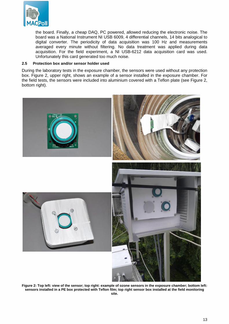
During the laboratory tests in the exposure chamber, the sensors were used without any protection box. Figure 2, upper right, shows an example of a sensor installed in the exposure chamber. For the field tests, the sensors were included into aluminium covered with a Teflon plate (see Figure 2, bottom right).
Figure 2: Top left: view of the sensor; top right: example of ozone sensors in the exposure chamber; b ottom left: sensors installed in a PE box protected with Teflon f ilm; top right sensor box installed at the field mo nitoring
site.
14
3 Scope of validation
The aim of this study was to demonstrate whether or not the sensor satisfies the Data Quality Objective (DQO) for O3 Indicative Methods at the O3 target level (LV). The following conditions apply:
• the DQO consists of a relative expanded uncertainty of 30 % in the region of the Target Value (LV)
• the LV corresponds to 120 µg/m³ or 60 nmol/mol • the LV is defined as an 8-hour mean computed from hourly averages. Consequently, an
averaging time of one hour is mandatory. Other important values defined in the Directive consist of the AOT40 [2], 40 µg/m³ (20 nmol/mol), the information and alert thresholds (IT/AT): 180 µg/m³ (90 nmol/mol) and 240 µg/m³ (120 nmol/mol), respectively.
• it was planned to validate the sensor in the following micro-environment: at background stations in rural areas since they corresponds to zones where O3 monitoring is mandatory.
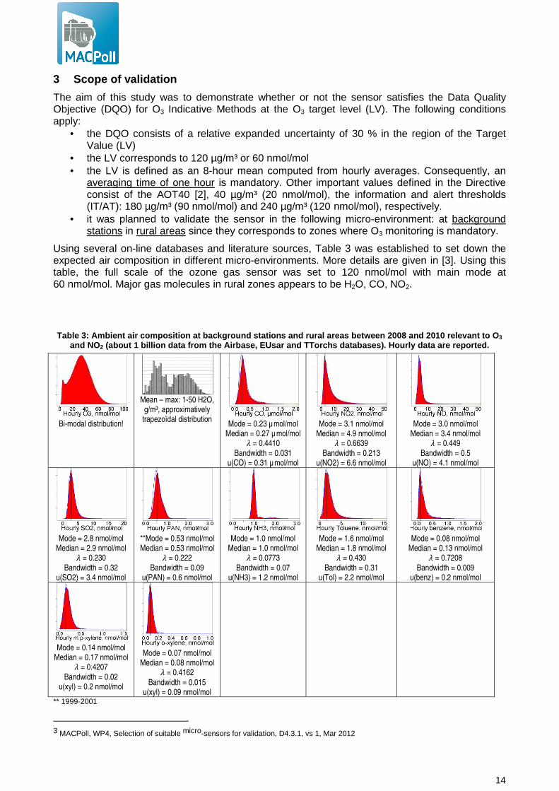
Using several on-line databases and literature sources, Table 3 was established to set down the expected air composition in different micro-environments. More details are given in [3]. Using this table, the full scale of the ozone gas sensor was set to 120 nmol/mol with main mode at 60 nmol/mol. Major gas molecules in rural zones appears to be H2O, CO, NO2.
Table 3: Ambient air composition at background stat ions and rural areas between 2008 and 2010 relevant to O3 and NO2 (about 1 billion data from the Airbase, EUsar and T Torchs databases). Hourly data are reported.
Bi-modal distribution!
Mean – max: 1-50 H2O,
g/m³, approximatively trapezoïdal distribution
Mode = 0.23 µ mol/mol Median = 0.27 µ mol/mol
� = 0.4410 Bandwidth = 0.031
u(CO) = 0.31 µ mol/mol
Mode = 3.1 nmol/mol
Median = 4.9 nmol/mol � = 0.6639
Bandwidth = 0.213 u(NO2) = 6.6 nmol/mol
Mode = 3.0 nmol/mol
Median = 3.4 nmol/mol � = 0.449
Bandwidth = 0.5 u(NO) = 4.1 nmol/mol
Mode = 2.8 nmol/mol
Median = 2.9 nmol/mol � = 0.230
Bandwidth = 0.32 u(SO2) = 3.4 nmol/mol
**Mode = 0.53 nmol/mol Median = 0.53 nmol/mol
� = 0.222 Bandwidth = 0.09
u(PAN) = 0.6 nmol/mol
Mode = 1.0 nmol/mol
Median = 1.0 nmol/mol � = 0.0773
Bandwidth = 0.07 u(NH3) = 1.2 nmol/mol
Mode = 1.6 nmol/mol
Median = 1.8 nmol/mol � = 0.430
Bandwidth = 0.31 u(Tol) = 2.2 nmol/mol
Mode = 0.08 nmol/mol
Median = 0.13 nmol/mol � = 0.7208
Bandwidth = 0.009 u(benz) = 0.2 nmol/mol
Mode = 0.14 nmol/mol
Median = 0.17 nmol/mol � = 0.4207
Bandwidth = 0.02 u(xyl) = 0.2 nmol/mol
Mode = 0.07 nmol/mol
Median = 0.08 nmol/mol � = 0.4162
Bandwidth = 0.015 u(xyl) = 0.09 nmol/mol
** 1999-2001
3 MACPoll, WP4, Selection of suitable micro-sensors for validation, D4.3.1, vs 1, Mar 2012
15
It was observed that within Airbase data series, between 2008 and 2010, some pollutants presented a few low negative values (O3, NO, NO2...) for background rural stations. As this is a mistake; it was thought that these values may correspond to 0. Therefore, it was decided to add the corresponding negative values to the datasets.
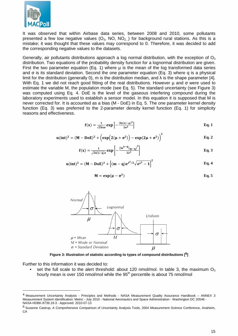
Generally, air pollutants distributions approach a log normal distribution, with the exception of O3 distribution. Two equations of the probability density function for a lognormal distribution are given. First the two parameter equation (Eq. 1) where µ is the mean of the log transformed data series and σ is its standard deviation. Second the one parameter equation (Eq. 3) where q is a physical limit for the distribution (generally 0), m is the distribution median, and λ is the shape parameter [4]. With Eq. 1 we did not reach good fitting of the real distributions. However µ and σ were used to estimate the variable M, the population mode (see Eq. 5). The standard uncertainty (see Figure 3) was computed using Eq. 4. DoE is the level of the gaseous interfering compound during the laboratory experiments used to establish a sensor model. In this equation it is supposed that M is never corrected for. It is accounted as a bias (M - DoE) in Eq. 5. The one parameter kernel density function (Eq. 3) was preferred to the 2-parameter density kernel function (Eq. 1) for simplicity reasons and effectiveness.
���� = �
√������� �− �������
���� Eq. 1
(��)� = � − ����� + �������� + ���� − ������+ ����� Eq. 2
���� = �
���������� �− ����� ���� �
�
���� Eq. 3
(��)� = � − ����� + ��� − ����� �⁄ ���� − ��� Eq. 4
= ����� − ��� Eq. 5
Figure 3: Illustration of statistic according to ty pes of compound distributions [ 5]
Further to this information it was decided to: • set the full scale to the alert threshold: about 120 nmol/mol. In table 3, the maximum O3
hourly mean is over 150 nmol/mol while the 95th percentile is about 75 nmol/mol
4 Measurement Uncertainty Analysis - Principles and Methods - NASA Measurement Quality Assurance Handbook – ANNEX 3 Measurement System Identification: Metric - July 2010 - National Aeronautics and Space Administration - Washington DC 20546 - NASA-HDBK-8739.19-3 - Approved: 2010-07-13 5 Suzanne Castrup, A Comprehensive Comparison of Uncertainty Analysis Tools, 2004 Measurement Science Conference, Anaheim, CA
16
• to check the interference of abundant compounds: H2O, CO, NO2/NO, NH3, and SO2 to a lesser extent. PAN was not considered because it is too difficult to generate and control.
• the mean temperature and mean relative humidity were set to 22 °C and 60 %, respectively.
It is worth reminding that before using the sensor based on the validation data included in this report, it should be ascertained that the sensor is applied in the same configuration in which it was tested here. This requires using the same data acquisition and processing, the same protection box and calibration type. The sensor shall be submitted to the same regime of QA/QC as during evaluation. In addition, it is strongly recommended that sensors results are periodically compared side-by-side using the reference method.
4 Literature review:
Category under which the gas sensor falls: • Sensors for which the relationship between sensor response and the tested gaseous
compound is not well established. Therefore, this study aims at setting up a model equation for the sensor and estimating the resulting measurement uncertainty.
• However, the manufacturer does indicate a sensitivity about 0.800 mv/(nmol/mol) for the measuring electrode (OP1) and about 200 mV for the zero electrode (OP2). This suggests a linear model of the sensor response versus O3.
• Apart from the subtraction of OP2 to OP1, the company does not supply information about any relevant correction for gaseous interfering compounds, temperature and humidity that should be applied to transform the sensor responses into O3 concentrations.
• In addition to the sensitivity written on each sensor bag, the manufacturer provides a data sheet with characteristics of the O3-B4 sensor (see 11 in appendix). Metrological parameters (time response, drift, noise linearity, range of O3 measurement and lifetime) can be found. Cross sensitivities to other gaseous compounds are given even though at high level (in µmol/mol). The data sheet also gives some data for the effect of temperature and humidity on the sensor response.
The following information was asked to the manufacturer. Answers to this questions can partly be found in annex 1.
• Available and public information regarding the sensors; • Chemical/physical principle on which the sensor is based; • Identification of sensor model and version of the sensors, method of preparation; • Relationship between the raw sensor signal and the calculated concentration of air
pollutants, relevant data treatment, possible model equation or calibration method; • Any available details regarding: limits of detection/quantification, (hot/cold) warming time,
response time, drift over time, temperature/humidity/pressure effect, interference from other compounds-
• Validation data carried out in lab experiments and/or under field conditions. • Common uses of the sensors.
No info was found on the internet about the performance of this sensor. However, a recent publication presents information of αSense sensors performances for CO, NO and NO2 [6]. This publication does not evaluate the αSense O3 sensors.
6 M.I. Mead, O.A.M. Popoola, G.B. Stewart, P. Landshoff, M. Calleja, M. Hayes, et al., The use of electrochemical sensors for monitoring urban air quality in low-cost, high-density networks, Atmospheric Environment. 70 (2013) 186–203.
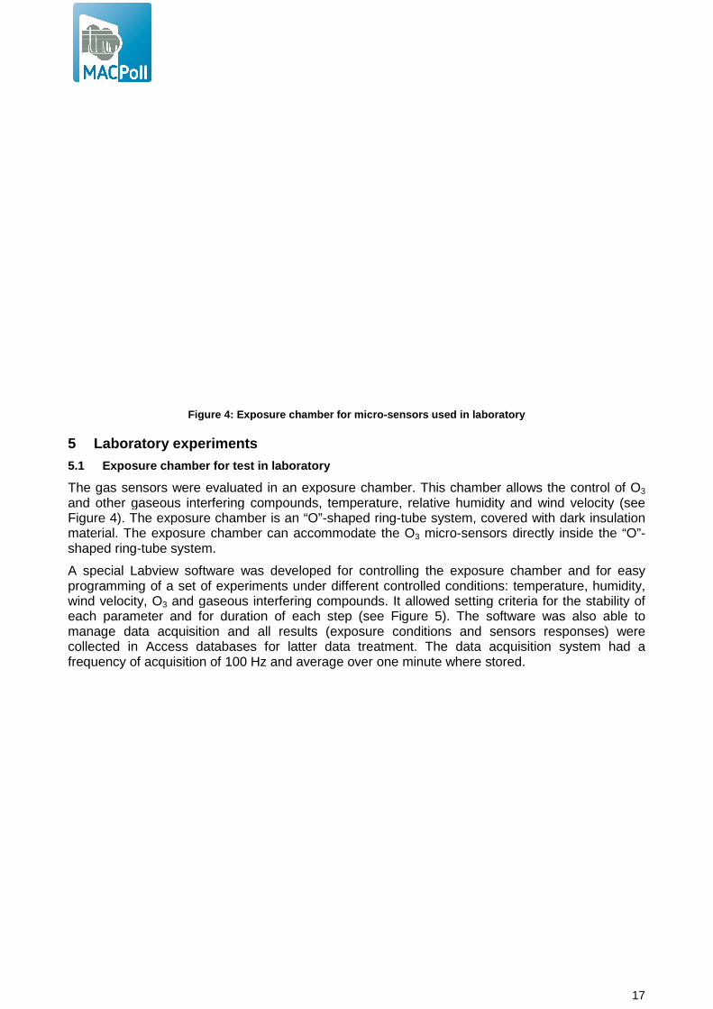
Figure 4 : Exposure chamber for micro
5 Laboratory experiments
5.1 Exposure chamber for test in laboratory
The gas sensors were evaluated in an exposure chamber. This chamber allows the control of and other gaseous interfering compounds, temperature, relative humidity and wind velocity Figure 4). The exposure chamber is an “O”material. The exposure chamber can accommodate theshaped ring-tube system.
A special Labview software was developed for controlling the exposure chamber and for easy programming of a set of experiments under different controlled conditions: temperature, humidity,wind velocity, O3 and gaseous interfering compounds. It allowed setting criteria for the stability of each parameter and for duration of each step (see manage data acquisition and all results (exposure conditions and sensors responses) were collected in Access databases for latter data treatment. The data acquisition system had a frequency of acquisition of 100 Hz and average ov
: Exposure chamber for micro -sensors used in l aboratory
Exposure chamber for test in laboratory
The gas sensors were evaluated in an exposure chamber. This chamber allows the control of and other gaseous interfering compounds, temperature, relative humidity and wind velocity
). The exposure chamber is an “O”-shaped ring-tube system, covered with dark insulation material. The exposure chamber can accommodate the O3 micro-sensors directly inside the “O”
A special Labview software was developed for controlling the exposure chamber and for easy programming of a set of experiments under different controlled conditions: temperature, humidity,
and gaseous interfering compounds. It allowed setting criteria for the stability of each parameter and for duration of each step (see Figure 5). The software was also able to manage data acquisition and all results (exposure conditions and sensors responses) were collected in Access databases for latter data treatment. The data acquisition system had a frequency of acquisition of 100 Hz and average over one minute where stored.
17
aboratory
The gas sensors were evaluated in an exposure chamber. This chamber allows the control of O3 and other gaseous interfering compounds, temperature, relative humidity and wind velocity (see
tube system, covered with dark insulation sensors directly inside the “O”-
A special Labview software was developed for controlling the exposure chamber and for easy programming of a set of experiments under different controlled conditions: temperature, humidity,
and gaseous interfering compounds. It allowed setting criteria for the stability of software was also able to
manage data acquisition and all results (exposure conditions and sensors responses) were collected in Access databases for latter data treatment. The data acquisition system had a
er one minute where stored.
18
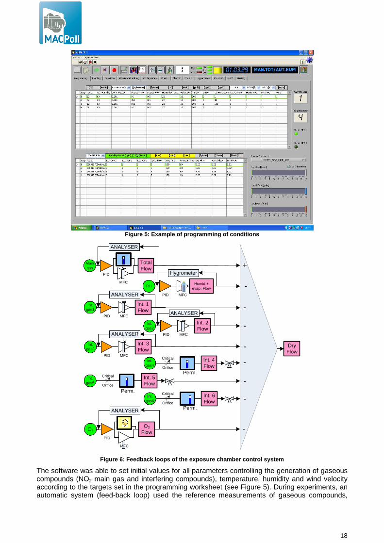
Figure 5: Example of programming of conditions
Int. 1Flow
MFC
Int. gas1
PID
ANALYSER
Int. 2Flow
MFC
Int. gas2
PID
ANALYSER
Humid + evap. Flow
MFC
RH
PID
Hygrometer
Int. 3Flow
MFC
Int. gas3
PID
ANALYSER
Int. 4Flow
Int. gas4
Critical
OrificePerm.
Int. 5Flow
Int. gas5
Critical
Orifice
Perm.
Perm.
TotalFlow
MFC
Maingas
PID
ANALYSER
DryFlow
+
-
-
-
-
-
-
-
-
Int. 6Flow
Int. gas6
Critical
Orifice
O3
Flow
MFC
O3
PID
ANALYSER
Figure 6: Feedback loops of the exposure chamber co ntrol system
The software was able to set initial values for all parameters controlling the generation of gaseous compounds (NO2 main gas and interfering compounds), temperature, humidity and wind velocity according to the targets set in the programming worksheet (see Figure 5). During experiments, an automatic system (feed-back loop) used the reference measurements of gaseous compounds,
19
temperature, humidity and wind speed to auto-correct the gas mixture generation system, temperature controlling cryostat and wind velocity to reach the target conditions (see the logical graph in Figure 6 and Figure 5).
5.2 Gas mixture generation system
For generating O3, two MicroCal 5000 Umwelttechnik MCZ Gmbh (G) generators were used. These generators are equipped with UV lamps placed in thermo insulted chamber whose UV beam is controlled by a regulated current intensity. The UV lamp dissociated O2 molecules into activated O* atoms that later combined with O2 molecule to form O3. The quantity of O2 depends on the intensity of the current applied to the UV lamp and the total flow of zero air of the generator which was adjusted by a mass flow controller and controlled by the exposure chamber LabView software. Prior to experiment, the mass flow controllers were calibrated against a Primary Flow Calibrator Gilian Gilibrator 2. The ozone mixtures generated by the MicroCals were calibrated against the NIST primary O3 photometer of the ERLAP laboratory.
Mixtures of gaseous interference were generated with an in-house designed Permeation system, using NH3, NO2, SO2 and HNO3 permeation tubes from KinTec (G) and Calibrage (F) that were weighed every 3 weeks. CO mixtures were directly generated by dynamic dilution from highly concentrated cylinders from Air Liquide.
For the response time experiment, the controlled conditions in the exposure chamber shall be established after a few minutes. Seen the internal volume of the exposure chamber (about 120 L), it was decided to use the automatic bench that ERLAP uses for the European inter-comparison exercises of the National Reference Laboratories of Air Pollution [7] that can generated mixture with a flow of about 100 L/min.
5.3 Reference methods of measurements
5.3.1 Methods
O3 was monitored using a Thermo Environment TEI 49C UV-photometer. The analyser was calibrated before the experiments using an O3 primary standard. It consists of a TEI Model 49 C Primary Standard, Thermo Environmental Instruments cross-checked against a long-path UV photometer (National Institute of Standards and Technology, reference photometer n° 42, USA).
Other gaseous compounds were recorded to ease understanding sensors results:
• NO/NOx/NO2: Thermo Environment 42 C chemiluminescence analyser, calibrated against a permeation system for NO2 and a NO working standard consisting of a gas cylinder at low concentration (down to 50 nmol/mol) certified against a Primary Reference Material of NMI VSL - NL
• SO2: Environment SA AF 21 M, calibrated with a working standard consisting of gas cylinder at low concentration (down to 50 nmol/mol) certified against a Primary Reference Material of NMI VSL - NL. The calibration of the analyser was confirmed by cross-checking with a permeation method.
• CO: Thermo Environment 48i-TLE NDIR analyser, calibrated with a CO working standard consisting of a gas cylinder at low concentration (down to 1 µmol/mol) certified against a Primary Reference Material of NMI VSL - NL.
• CO2: an infrared sensor, Gascard NG 0-1000 µmol/mol (Edinburg Sensors – UK) was used. This sensor includes pressure correction and temperature compensation. The sensor was calibrated with a CO2 cylinder (369 ppm for Air Liquide) and zero air obtained from an ultra pure Nitrogen cylinder.
• Analyser of NH3 Ammonia Analyzer, Model 17i (courtesy of monitoring network of Bolzano/Bozen – Italy)
7 M. Barbiere and F. Lagler, Evaluation of the Laboratory Comparison Exercise for SO2, CO, O3, NO and NO2, 11th-14th June 2012, EUR 25536, ISBN 978-92-79-26844-1, ISSN 1831-9424, doi:10.2788/52649, ftp://ftp_erlap_ro:3rlapsyst3m@s-jrciprvm-ftp-
ext.jrc.it/ERLAPDownload.htm
20
The sampling line of each gas analyser was equipped with a Naflyon dryer to avoid interference from water vapour on O3, NOx, SO2 and CO analyser.
In addition, some other parameters were recorded and/or controlled using: • Three refrigerated/heating circulators were used to regulate the temperature of the
exposure chamber. One cryostat (Julabo (G) Model SP-FP50) was used to control the temperature inside the exposure chamber, another one (Julabo (G) Model HE-FP50) for the surface of the O-shaped glass tube and the last one (Julabo (G) Model HE-FP50) was devoted to the control of temperature of the humid and dry air flows. These cryostats used a laboratory calibrated pt-100 probe placed inside the exposure chamber.
• Two KZC 2/5 sensors from TERSID-It (one with ISO 17025 certificate) were used to control temperature and relative humidity. One sensor was used to monitor in real-time using our Labview software, the second one was used to register these parameter.
• One Testo 445 sensor (Testoterm – G) with a temperature and relative humidity probe was used as a control interface to check values inside the chamber.
• One Testo 452 sensor (Testoterm – G) with a temperature and relative humidity probe was used as a reference sensor and to monitor temperature and relative humidity.
• One wind velocity probes based on hot-wire technology was use to monitor wind velocity during tests.
• One pressure gauge DPI 261 from Druck (G) was used to monitor pressure inside the exposure chamber
• Fan ventilator placed in the chamber, Papst (G) model, DV6224, 540 m³/hr.
• An in-house developed permeation system able to accommodate 8 permeation cells with carrier flows about 200 ml/min with critical orifices (Calibrage SA, (F)). Each permeation cell was dipped in a water bath consisted (Haake (G) W26 Thermostatic Circulating Water Bath with Haake E8 Controller). The temperature of each cell was set at 40 °C. The permeation tubes were weighed every three weeks. The permeation cells were filled with NO2, SO2, NH3 and HNO3 permeation tubes manufactured by KinTec (G) and Calibrage (F).
5.3.2 Quality control
During the experiments, the O3 analyser was monthly checked using a portable O3 generator SYCOS KTO 3 (Ansyco, GmbH - G) certified against the laboratory primary standard (NIST n°42). The NO2, SO2 and CO analysers were calibrated once a month using cylinders certified by the ERLAP laboratory. ERLAP is ISO-17025 accredited (ACCREDIA-IT, n°1362) for the measurement of O3, NO2, SO2 and CO according to EN 14625:2012, EN 14211:2012, EN 14212:2012 and EN 14626:2012, respectively.
5.3.3 Homogeneity
Several tests were performed to confirm the homogeneity of exposure conditions in the chamber at several positions in the exposure chamber.
6 Metrological parameters
6.1 Response time
The response time of sensors, t90, was computed by estimating t0-90 and t90-0 (the time needed by the sensor to reach 90 % of the final stable value or 0), after a sharp change of test gas level from 0 to 80 % of the full scale (FS) (rise time) and from 80 % of FS to 0 (fall time). Four determinations of rise and fall t90 were performed as shows Table 4. The averaging time of the O3 TECO 49C analyser was set to 60 sec in order to get a fast response of the reference analyser.
Table 4: Experiments for the determination of the re sponse time of sensors
Step Test gas RH T Interference Notes
21
1 90 nmol/mol 60 % 22 °C none Until stable response
2 0 nmol/mol 60 % 22 °C none Until stable response
3 90 nmol/mol 60 % 22 °C none Until stable response
4 0 nmol/mol 60 % 22 °C none Until stable response
5 90 nmol/mol 60 % 22 °C none Until stable response
6 0 nmol/mol 60 % 22 °C none Until stable response
7 90 nmol/mol 60 % 22 °C none Until stable response
8 0 nmol/mol 60 % 22 °C none Until stable response
9 90 nmol/mol 60 % 22 °C none Until stable response
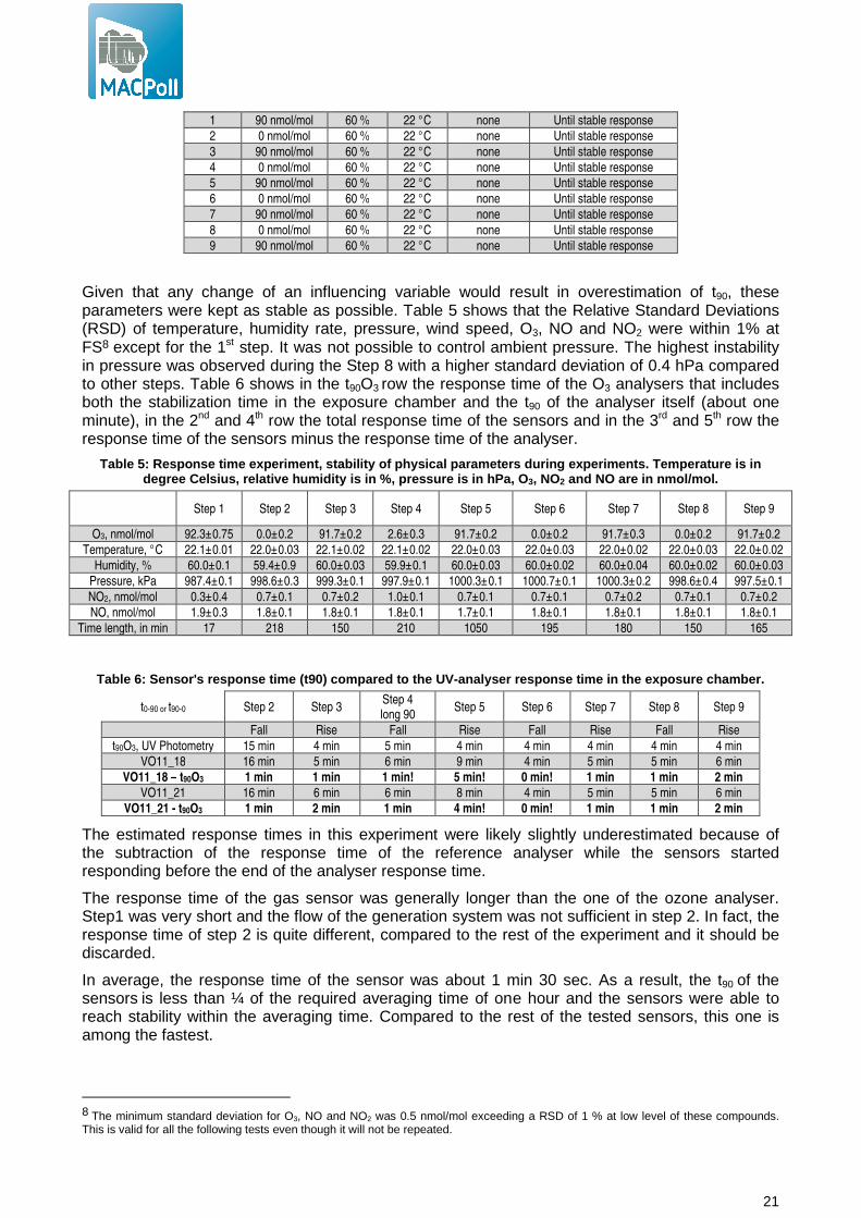
Given that any change of an influencing variable would result in overestimation of t90, these parameters were kept as stable as possible. Table 5 shows that the Relative Standard Deviations (RSD) of temperature, humidity rate, pressure, wind speed, O3, NO and NO2 were within 1% at FS8 except for the 1st step. It was not possible to control ambient pressure. The highest instability in pressure was observed during the Step 8 with a higher standard deviation of 0.4 hPa compared to other steps. Table 6 shows in the t90O3 row the response time of the O3 analysers that includes both the stabilization time in the exposure chamber and the t90 of the analyser itself (about one minute), in the 2nd and 4th row the total response time of the sensors and in the 3rd and 5th row the response time of the sensors minus the response time of the analyser.
Table 5: Response time experiment, stability of phy sical parameters during experiments. Temperature is in degree Celsius, relative humidity is in %, pressure is in hPa, O 3, NO2 and NO are in nmol/mol.
Step 1 Step 2 Step 3 Step 4 Step 5 Step 6 Step 7 Step 8 Step 9
O3, nmol/mol 92.3±0.75 0.0±0.2 91.7±0.2 2.6±0.3 91.7±0.2 0.0±0.2 91.7±0.3 0.0±0.2 91.7±0.2
Temperature, °C 22.1±0.01 22.0±0.03 22.1±0.02 22.1±0.02 22.0±0.03 22.0±0.03 22.0±0.02 22.0±0.03 22.0±0.02
Humidity, % 60.0±0.1 59.4±0.9 60.0±0.03 59.9±0.1 60.0±0.03 60.0±0.02 60.0±0.04 60.0±0.02 60.0±0.03
Pressure, kPa 987.4±0.1 998.6±0.3 999.3±0.1 997.9±0.1 1000.3±0.1 1000.7±0.1 1000.3±0.2 998.6±0.4 997.5±0.1
NO2, nmol/mol 0.3±0.4 0.7±0.1 0.7±0.2 1.0±0.1 0.7±0.1 0.7±0.1 0.7±0.2 0.7±0.1 0.7±0.2
NO, nmol/mol 1.9±0.3 1.8±0.1 1.8±0.1 1.8±0.1 1.7±0.1 1.8±0.1 1.8±0.1 1.8±0.1 1.8±0.1
Time length, in min 17 218 150 210 1050 195 180 150 165
Table 6: Sensor's response time (t90) compared to th e UV-analyser response time in the exposure chamber .
t0-90 or t90-0 Step 2 Step 3 Step 4 long 90
Step 5 Step 6 Step 7 Step 8 Step 9
Fall Rise Fall Rise Fall Rise Fall Rise
t90O3, UV Photometry 15 min 4 min 5 min 4 min 4 min 4 min 4 min 4 min
VO11_18 16 min 5 min 6 min 9 min 4 min 5 min 5 min 6 min
VO11_18 – t90O3 1 min 1 min 1 min! 5 min! 0 min! 1 min 1 min 2 min
VO11_21 16 min 6 min 6 min 8 min 4 min 5 min 5 min 6 min
VO11_21 - t90O3 1 min 2 min 1 min 4 min! 0 min! 1 min 1 min 2 min
The estimated response times in this experiment were likely slightly underestimated because of the subtraction of the response time of the reference analyser while the sensors started responding before the end of the analyser response time.
The response time of the gas sensor was generally longer than the one of the ozone analyser. Step1 was very short and the flow of the generation system was not sufficient in step 2. In fact, the response time of step 2 is quite different, compared to the rest of the experiment and it should be discarded.
In average, the response time of the sensor was about 1 min 30 sec. As a result, the t90 of the sensors is less than ¼ of the required averaging time of one hour and the sensors were able to reach stability within the averaging time. Compared to the rest of the tested sensors, this one is among the fastest.
8 The minimum standard deviation for O3, NO and NO2 was 0.5 nmol/mol exceeding a RSD of 1 % at low level of these compounds. This is valid for all the following tests even though it will not be repeated.
22
In average, the sensors were faster in fall condition (about 45 sec) than in rise condition (about 2 min 15 sec). Even though, this difference exceeds 10 %, it is assumed that this difference will not affect significantly an hourly average at rural site where ozone concentrations slowly changes.
In the following validation experiments, all steps should last for at least 2.25 x 4 = 9 minutes plus the stabilisation time of the exposure chamber. Because of other sensors, it was decided to have each lasting for 150 minutes, well longer that the response time of the sensors.
The sensors were found quite suitable for mobile monitoring, being able to deliver independent 9-minute averages. However, micro-environment where air pollutants changes with a periodicity of a few minutes (e. g. with rapid indoor/outdoor moves) are not advised.
6.2 Pre calibration
The objective of this experiment was to check if the transformation of sensor response into air pollutant levels does not include any bias at the mean temperature and relative humidity.
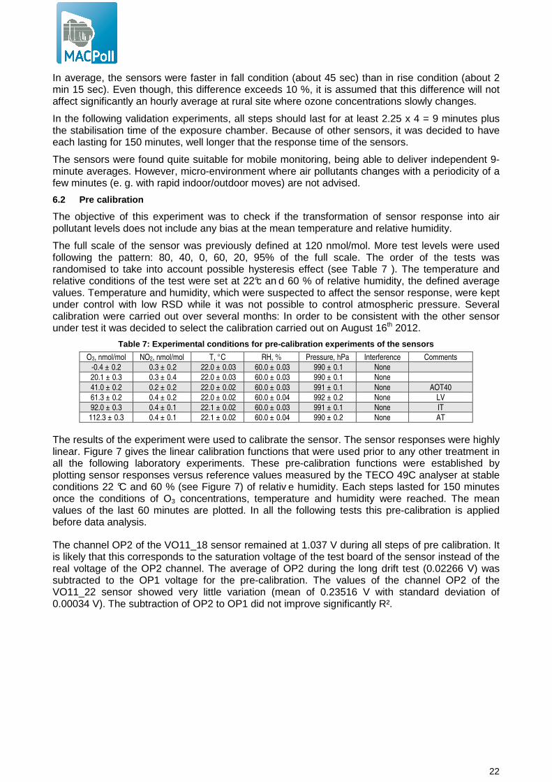
The full scale of the sensor was previously defined at 120 nmol/mol. More test levels were used following the pattern: 80, 40, 0, 60, 20, 95% of the full scale. The order of the tests was randomised to take into account possible hysteresis effect (see Table 7 ). The temperature and relative conditions of the test were set at 22°c an d 60 % of relative humidity, the defined average values. Temperature and humidity, which were suspected to affect the sensor response, were kept under control with low RSD while it was not possible to control atmospheric pressure. Several calibration were carried out over several months: In order to be consistent with the other sensor under test it was decided to select the calibration carried out on August 16th 2012.
Table 7: Experimental conditions for pre-calibration experiments of the sensors
O3, nmol/mol NO2, nmol/mol T, °C RH, % Pressure, hPa Interference Comments
-0.4 ± 0.2 0.3 ± 0.2 22.0 ± 0.03 60.0 ± 0.03 990 ± 0.1 None
20.1 ± 0.3 0.3 ± 0.4 22.0 ± 0.03 60.0 ± 0.03 990 ± 0.1 None
41.0 ± 0.2 0.2 ± 0.2 22.0 ± 0.02 60.0 ± 0.03 991 ± 0.1 None AOT40
61.3 ± 0.2 0.4 ± 0.2 22.0 ± 0.02 60.0 ± 0.04 992 ± 0.2 None LV
92.0 ± 0.3 0.4 ± 0.1 22.1 ± 0.02 60.0 ± 0.03 991 ± 0.1 None IT
112.3 ± 0.3 0.4 ± 0.1 22.1 ± 0.02 60.0 ± 0.04 990 ± 0.2 None AT
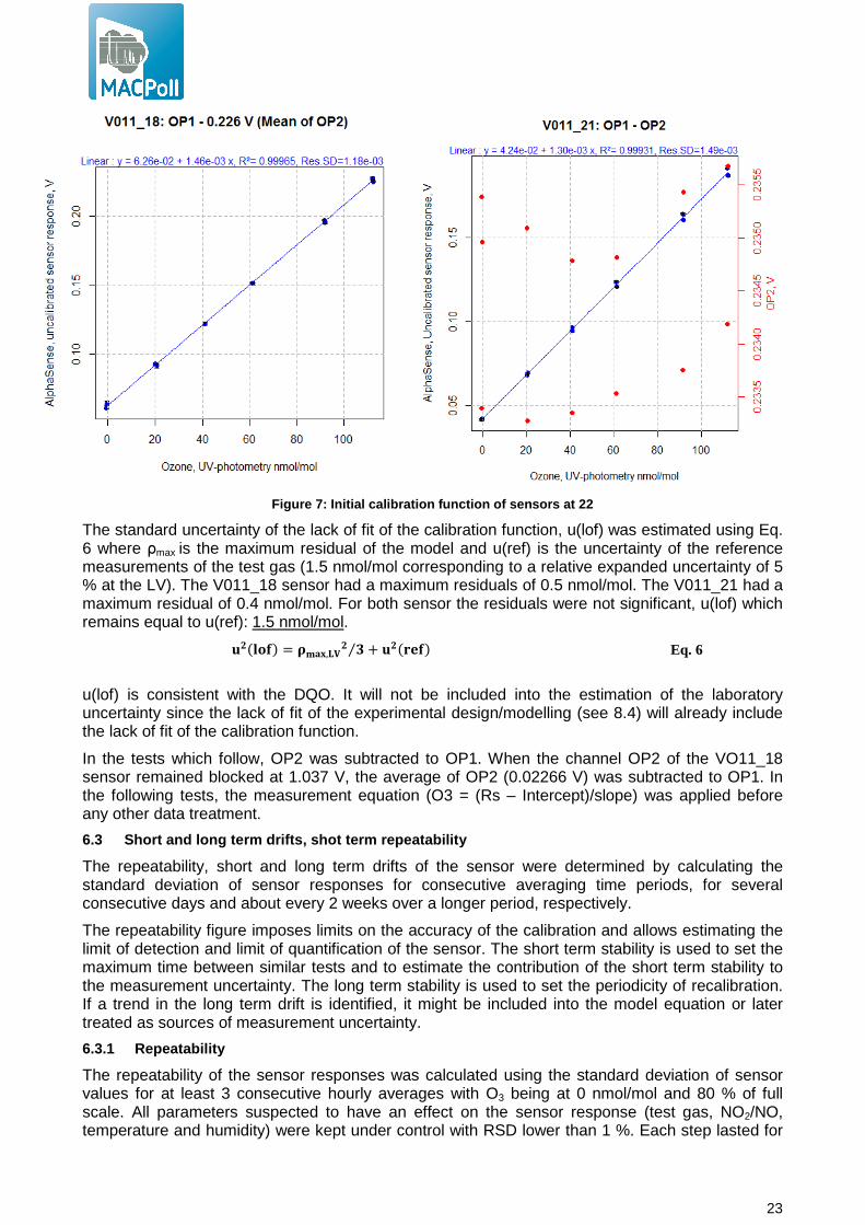
The results of the experiment were used to calibrate the sensor. The sensor responses were highly linear. Figure 7 gives the linear calibration functions that were used prior to any other treatment in all the following laboratory experiments. These pre-calibration functions were established by plotting sensor responses versus reference values measured by the TECO 49C analyser at stable conditions 22 °C and 60 % (see Figure 7) of relativ e humidity. Each steps lasted for 150 minutes once the conditions of O3 concentrations, temperature and humidity were reached. The mean values of the last 60 minutes are plotted. In all the following tests this pre-calibration is applied before data analysis.
The channel OP2 of the VO11_18 sensor remained at 1.037 V during all steps of pre calibration. It is likely that this corresponds to the saturation voltage of the test board of the sensor instead of the real voltage of the OP2 channel. The average of OP2 during the long drift test (0.02266 V) was subtracted to the OP1 voltage for the pre-calibration. The values of the channel OP2 of the VO11_22 sensor showed very little variation (mean of 0.23516 V with standard deviation of 0.00034 V). The subtraction of OP2 to OP1 did not improve significantly R².
23
Figure 7: Initial calibration function of sensors a t 22
The standard uncertainty of the lack of fit of the calibration function, u(lof) was estimated using Eq. 6 where ρmax is the maximum residual of the model and u(ref) is the uncertainty of the reference measurements of the test gas (1.5 nmol/mol corresponding to a relative expanded uncertainty of 5 % at the LV). The V011_18 sensor had a maximum residuals of 0.5 nmol/mol. The V011_21 had a maximum residual of 0.4 nmol/mol. For both sensor the residuals were not significant, u(lof) which remains equal to u(ref): 1.5 nmol/mol.
������ = ����,��� ⁄ + ��"��� Eq. 6
u(lof) is consistent with the DQO. It will not be included into the estimation of the laboratory uncertainty since the lack of fit of the experimental design/modelling (see 8.4) will already include the lack of fit of the calibration function.
In the tests which follow, OP2 was subtracted to OP1. When the channel OP2 of the VO11_18 sensor remained blocked at 1.037 V, the average of OP2 (0.02266 V) was subtracted to OP1. In the following tests, the measurement equation (O3 = (Rs – Intercept)/slope) was applied before any other data treatment.
6.3 Short and long term drifts, shot term repeatabi lity
The repeatability, short and long term drifts of the sensor were determined by calculating the standard deviation of sensor responses for consecutive averaging time periods, for several consecutive days and about every 2 weeks over a longer period, respectively.
The repeatability figure imposes limits on the accuracy of the calibration and allows estimating the limit of detection and limit of quantification of the sensor. The short term stability is used to set the maximum time between similar tests and to estimate the contribution of the short term stability to the measurement uncertainty. The long term stability is used to set the periodicity of recalibration. If a trend in the long term drift is identified, it might be included into the model equation or later treated as sources of measurement uncertainty.
6.3.1 Repeatability
The repeatability of the sensor responses was calculated using the standard deviation of sensor values for at least 3 consecutive hourly averages with O3 being at 0 nmol/mol and 80 % of full scale. All parameters suspected to have an effect on the sensor response (test gas, NO2/NO, temperature and humidity) were kept under control with RSD lower than 1 %. Each step lasted for
24
150 minutes, the period determined in the response time experiment (see 5.2). The calculation of the standard deviation of repeatability was carried out using the following equation:
1
)( 2
−−
= ∑N
RRs i
r (Eq. 7)
Where Ri is each measurement, �� is the mean sensor response and N the number of measurements. These experiments took place between 19 and 21 Sep. 2012.
Table 8: Results of the repeatability of hourly val ues at 0 and at 90 nmol/mol of O 3 with mean and standard deviation
O3 NO2 NO CO T Rel. Hum. P_hPa V011_18 V011_21
nmol/mol nmol/mol nmol/mol nmol/mol °C % hPa nmol/mol nmol/mol
Mean ± s (n=4) 0.0 ± 0,1 0,7 ± 0,0 1,7 ± 0,1 250 ± 13,0 22,0 ± 0,0 59,1 ± 0,9 993,5 ± 5.1 0.0 ± 2.0 0.6 ± 2.5
Mean ± s (n=16) 91,7 ± 0,0 0,7 ± 0,0 1,7 ± 0,0 267 ± 13 22,0 ± 0,0 60,0 ± 0,0 1000 ± 0,5 93.2 ± 0.4 94.2 ± 0.3
The results of the repeatability experiment are given in Table 8. One can observe that the sensors showed more variability at zero O3 than when exposed to high O3. The repeatability of the sensor measurements, the likely difference between two measurements made under repeatability conditions, was computed as 2√2�� where sr is the standard deviation of repeatability for 90 nmol/mol of O3. In average, this gave a repeatability of:
• 1.0 nmol/mol for the sensor V011_18 • 0.8 nmol/mol for the sensor V011_21.
The limits of detection and limits of quantification, were estimated as 3s and 10s where s is the standard deviation of repeatability for the 0-nmol/mol O3 level:
• 6.0 and 20.0 nmol/mol for the V011_18. • 7.6 and 25.3 nmol/mol for the V011_21.
These high limits were likely driven by the relative variability of the OP1/OP2 channels at zero O3.
6.3.2 Short term drift
For the short term drift, a few measurements were carried out on several consecutive days (in fact with 12 to 36 hours between the first and the second measurements) at 0 nmol/mol, 50 % and 80 % of the LV. The averaging of sensor responses at 0, 60 and 90 nmol/nmol were calculated over the last hour of stable conditions of O3, temperature and relative humidity while each step lasted for 150 min long after stabilisation. For each successive steps, the maximum allowed deviation from targets was less than 2 nmol/mol for O3, 1°C and 1 % for O 3, temperature and relative humidity, respectively. These stability conditions were used throughout this study. The short term stability was estimated using Eq. 8.
#�� =∑ %&�,����� − &�,��� ��%!"� ' Eq. 8
where Rs are the sensor responses (calibrated as in 6.2) at 0, 60 and 90 nmol/mol at t0 (��,������) and 24 hours later (��,�����); N is the number of pairs of measurements. Experiments for which NO2 or NO were higher than 10 nmol/mol were not considered.
25
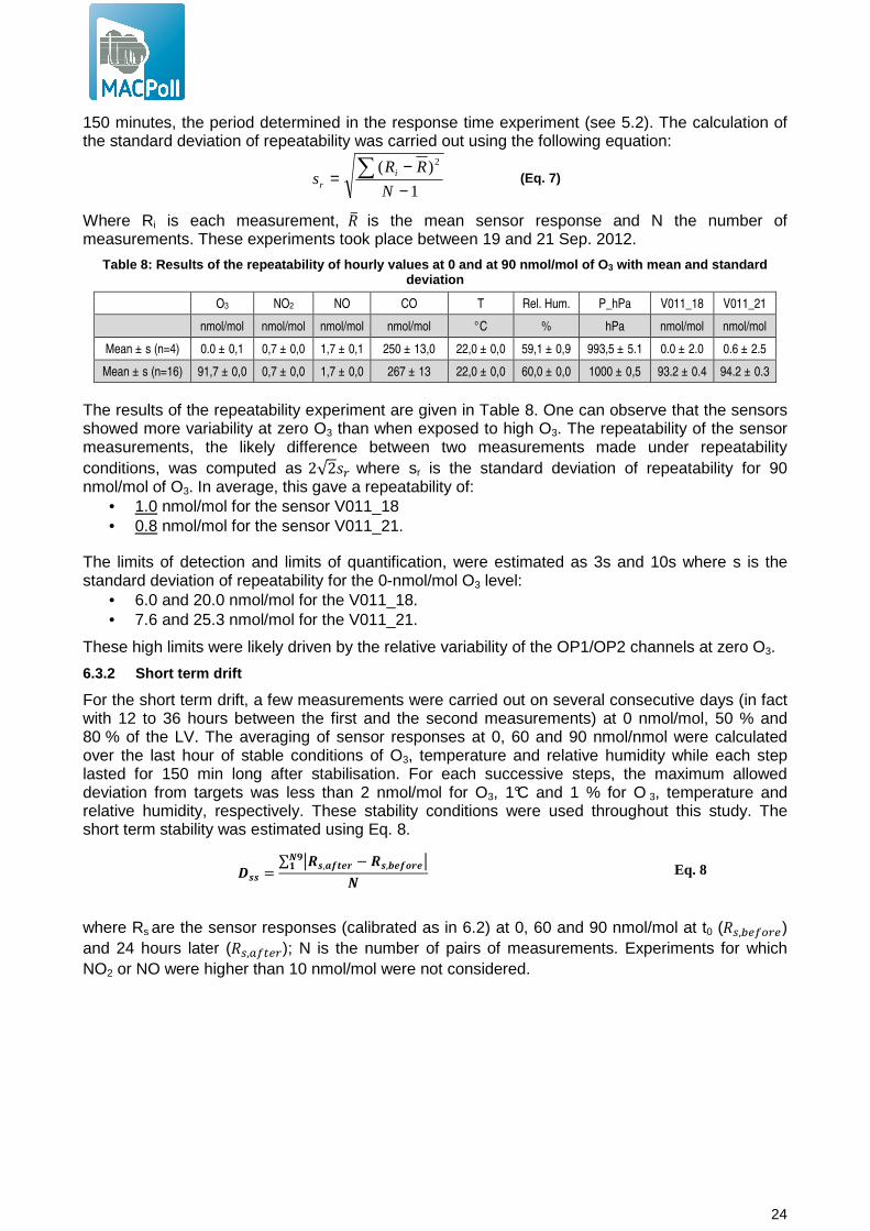
Figure 8 Short term drift of O 3, NO2, temperature and humidity in the exposure chamber during the short term
drift experiments
The tests took place between April 30th and November 13th 2012. During the experiment all parameters supposed to have an effect on the sensor response (O3, NO2, NO, CO, SO2, temperature, humidity, wind velocity ...) were kept under control. As written before, it is important to control them otherwise the variation of these parameters would be added to the sensor variability. The short term drifts of O3, NO2, temperature and humidity (not for the sensors), calculated according to Eq. 8, are given in Figure 8. It showed low variation for all parameters except for O3 at 0 nmol/mol (1.1 nmol/mol). Since O3 has a direct effect on the sensors, it was decided to subtract the short drift of O3 (Dss of O3) to the short drift of sensors (Dss of V011_18 and of V011_21). Similarly, the variance of O3 was subtracted to the variance of short drift of the sensors.
Table 9: Average conditions of exposure and short t erm drift of sensors during all experiments. The la st two columns give the short term stability Dss for the s ensors. All quoted values represent the standard de viation of
each parameter.
O3, nmol/mol NO2, nmol/mol T, °C RH, % Pressure, hPa Interference Dss V011_18,
nmol/mol Dss V011_21,
nmol/mol
0.2 ± 1.1 0.5 ± 0.2 22.1 ± 0.2 59.8 ± 0.4 993 ± 5.1 None 3.5 ± 3.7 (n=15) 2.6 ± 3.0 (n=23)
61.1 ± 0.2 0.5 ± 0.3 22.1 ± 0.1 59.8 ± 0.4 989 ± 3.1 None 0.9 ± 0.7 (n=10) 0.5 ± 0.5 (n=16)
91.7 ± 0.2 0.4 ± 0.4 22.1 ± 0.1 59.8 ± 0.5 994 ± 4.4 None 0.8 ± 0.6 (n=10) 0.4 ± 0.2 (n=15)
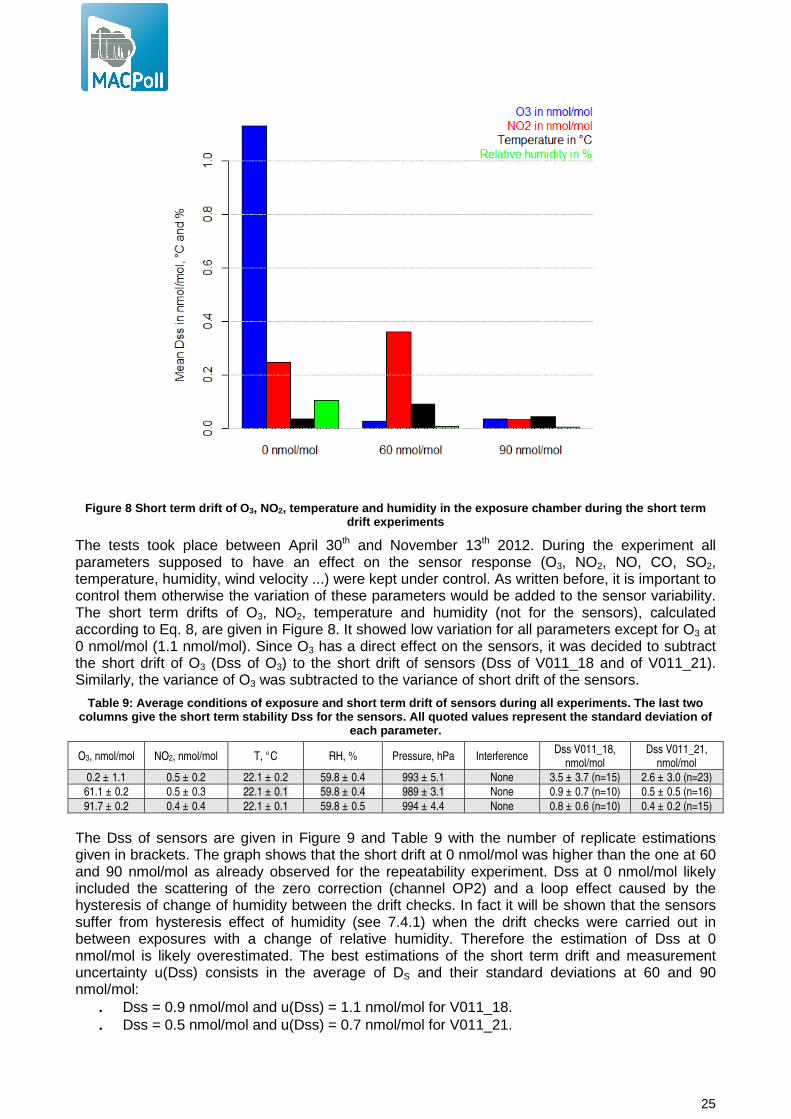
The Dss of sensors are given in Figure 9 and Table 9 with the number of replicate estimations given in brackets. The graph shows that the short drift at 0 nmol/mol was higher than the one at 60 and 90 nmol/mol as already observed for the repeatability experiment. Dss at 0 nmol/mol likely included the scattering of the zero correction (channel OP2) and a loop effect caused by the hysteresis of change of humidity between the drift checks. In fact it will be shown that the sensors suffer from hysteresis effect of humidity (see 7.4.1) when the drift checks were carried out in between exposures with a change of relative humidity. Therefore the estimation of Dss at 0 nmol/mol is likely overestimated. The best estimations of the short term drift and measurement uncertainty u(Dss) consists in the average of DS and their standard deviations at 60 and 90 nmol/mol:
• Dss = 0.9 nmol/mol and u(Dss) = 1.1 nmol/mol for V011_18. • Dss = 0.5 nmol/mol and u(Dss) = 0.7 nmol/mol for V011_21.
26
The contribution to the measurement uncertainty u(Dss) was calculated using Eq. 9 where si represents the standard deviation of the Dss at each concentration level.
���##� = �##� +
∑ ����#���
���
∑ ��������
Eq. 9
Dss (about 1.5 nmol/mol in average) is similar to the repeatability figure. In conclusion, a maximum duration of experiments of 48 hours (and more) can be accepted without fearing high short term drift.
Figure 9: Short term drift for sensors at three O 3 levels. Each bar represents the absolute mean diffe rences, Dss,
between sensor responses at t 0 and t 0+24 hrs, the error bars represent to the standard d eviation of Dss
6.3.3 Long term drift
For the long term drift, a similar approach as the one for short term drift was carried out measuring sensor response at 0, 60 and 90 nmol/mol during the experiment. The long term drift stability was estimated using the trends of the sensor responses from the beginning to the end of all laboratory experiment.
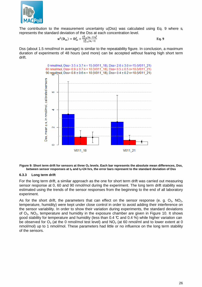
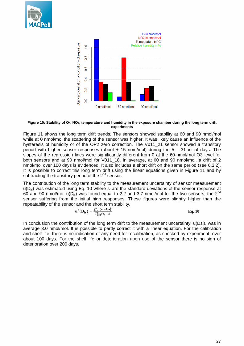
As for the short drift, the parameters that can effect on the sensor response (e. g. O3, NO2, temperature, humidity) were kept under close control in order to avoid adding their interference on the sensor variability. In order to show their variation during experiments, the standard deviations of O3, NO2, temperature and humidity in the exposure chamber are given in Figure 10. It shows good stability for temperature and humidity (less than 0.4 °C and 0.4 %) while higher variation can be observed for O3 (at the 0 nmol/mol test level) and NO2 (at 60 nmol/ml and to lower extent at 0 nmol/mol) up to 1 nmol/mol. These parameters had little or no influence on the long term stability of the sensors.
27
Figure 10: Stability of O 3, NO2, temperature and humidity in the exposure chamber during the long term drift
experiments
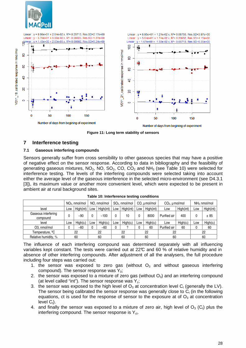
Figure 11 shows the long term drift trends. The sensors showed stability at 60 and 90 nmol/mol while at 0 nmol/mol the scattering of the sensor was higher. It was likely cause an influence of the hysteresis of humidity or of the OP2 zero correction. The V011_21 sensor showed a transitory period with higher sensor responses (about + 15 nom/mol) during the 5 – 31 initial days. The slopes of the regression lines were significantly different from 0 at the 60-nmol/mol O3 level for both sensors and at 90 nmol/mol for V011_18. In average, at 60 and 90 nmol/mol, a drift of 2 nmol/mol over 100 days is evidenced. It also includes a short drift on the same period (see 6.3.2). It is possible to correct this long term drift using the linear equations given in Figure 11 and by subtracting the transitory period of the 2nd sensor.
The contribution of the long term stability to the measurement uncertainty of sensor measurement u(Dls) was estimated using Eq. 10 where si are the standard deviations of the sensor response at 60 and 90 nmol/mo. u(Dls) was found equal to 2.2 and 3.7 nmol/mol for the two sensors, the 2nd sensor suffering from the initial high responses. These figures were slightly higher than the repeatability of the sensor and the short term stability.
����#� = ∑ ����#���
���
∑ ��������
Eq. 10
In conclusion the contribution of the long term drift to the measurement uncertainty, u(Dsl), was in average 3.0 nmol/mol. It is possible to partly correct it with a linear equation. For the calibration and shelf life, there is no indication of any need for recalibration, as checked by experiment, over about 100 days. For the shelf life or deterioration upon use of the sensor there is no sign of deterioration over 200 days.
28
Figure 11: Long term stability of sensors
7 Interference testing
7.1 Gaseous interfering compounds
Sensors generally suffer from cross sensibility to other gaseous species that may have a positive of negative effect on the sensor response. According to data in bibliography and the feasibility of generating gaseous mixtures, NO2, NO, SO2, CO, CO2 and NH3 (see Table 10) were selected for interference testing. The levels of the interfering compounds were selected taking into account either the average level of the gaseous interference in the selected micro-environment (see D4.3.1 [3]), its maximum value or another more convenient level, which were expected to be present in ambient air at rural background sites.
Table 10: Interference testing conditions
NO2, nmol/mol NO, nmol/mol SO2, nmol/mol CO, µ mol/mol CO2, µ mol/mol NH3, nmol/mol
level Low High(int) Low High(int) Low High(int) Low High(int) Low High(int) Low High(int)
Gaseous interfering compound
0 ~90 0 ~100 0 10 0 8000 Purified air 400 0 ± 85
level Low High(ct) Low High(ct) Low High(ct) Low High(ct) Low High(ct) Low High(ct)
O3, nmol/mol 0 ~60 0 ~60 0 ? 0 60 Purified air 60 0 60
Temperature, ºC 22 22 22 22 22 22
Relative humidity, % 60 60 60 60 60 60
The influence of each interfering compound was determined separately with all influencing variables kept constant. The tests were carried out at 22°C and 60 % of relative humidity and in absence of other interfering compounds. After adjustment of all the analysers, the full procedure including four steps was carried out:
1. the sensor was exposed to zero gas (without O3 and without gaseous interfering compound). The sensor response was Y0;
2. the sensor was exposed to a mixture of zero gas (without O3) and an interfering compound (at level called “int”). The sensor response was Yz;
3. the sensor was exposed to the high level of O3 at concentration level Ct (generally the LV). The sensor being calibrated the sensor response was generally close to Ct (in the following equations, ct is used for the response of sensor to the exposure at of O3 at concentration level Ct).
4. and finally the sensor was exposed to a mixture of zero air, high level of O3 (Ct) plus the interfering compound. The sensor response is Yct.
29
The sensors were exposed for a time period equal to one independent measurement to reach stability and then three independent measurements were taken. The level of the mixtures of the test gas and gaseous interfering compounds (apart from NH3 for which we relied on gravimetric values) were measured using reference methods of measurement with a low uncertainty of measurements (uncertainty of less than 5 %) traceable to (inter)nationally accepted standards (see 5.3).
The influence quantity of the gaseous interfering compounds at zero (Yint,z) and at level ct (Yint,ct) were calculated using Eq. 11 and Eq. 12. The influence quantity of the interferent, Yint,LV, at the LV of O3 is estimated using Eq. 13 where Ct is this time the high level of O3 in the exposure chamber. The standard uncertainty associated with the gaseous interference compound, u(int), is calculated according to Eq. 14 depending on the type of distribution of the gaseous interfering compound. If a rectangular distribution was assumed Ci,max and Ci,mini were the maximum and minimum value of the interfering compound present in the micro environment. Eq. 14 gives also the equation for normal distribution and log-normal distribution which follows the same ideas as in paragraph 3 about the distribution of air composition.
0int, YYY zz −= Eq. 11
tctct cYY −=int, Eq. 12
zt
zctLV YC
LVYYY int,int,int,int, )( +−= Eq. 13
Lognormal distribution: ����� = �%���,�&'
�� (� − ����� + ��� − ����� �⁄ ���� − ���) Normal distribution:����� = �%���,�
&'�� +�� − ����� + ,�-
Rectangular distribution: ����� = �%���,�&'
�� (�� −����� + �(�,���(�,��
����)
Eq. 14
����� = �%���, &'
�� (�� − ����� + �(�,���(�,��
����) or ����� = �%���,��
&'�� (�� − ����� + �(�,���(�,��
����) Eq. 15
Sometimes it was not possible to estimate Yint,z and/or Yint,ct. For example, it was not possible to estimate the interference of NO on O3 because of its oxidation in NO2 or sometimes Yint,z was doubtful because of the higher variability of the sensor at 0 nmol/mol of O3. In this case, the simple approach given in paragraph 8.5.6 of ISO 14956:2002 based on the determination of the sensitivity coefficient b (difference of sensor responses divided by the extent of the interfering compound level at one level) was applied. An example is given assuming a rectangular distribution of an interfering compound in Eq. 15. For other distributions, the same treatment as in Eq. 14 was applied.
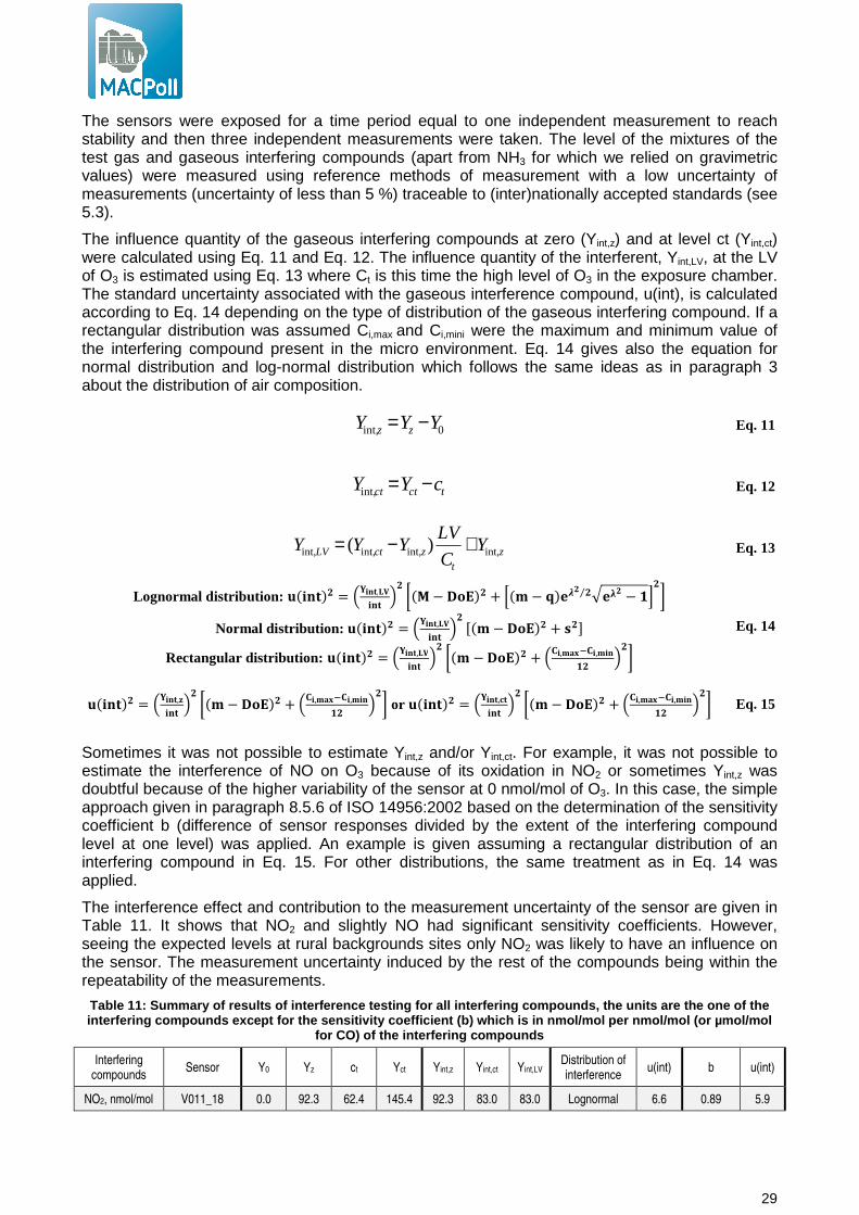
The interference effect and contribution to the measurement uncertainty of the sensor are given in Table 11. It shows that NO2 and slightly NO had significant sensitivity coefficients. However, seeing the expected levels at rural backgrounds sites only NO2 was likely to have an influence on the sensor. The measurement uncertainty induced by the rest of the compounds being within the repeatability of the measurements.
Table 11: Summary of results of interference testing for all interfering compounds, the units are the o ne of the interfering compounds except for the sensitivity co efficient (b) which is in nmol/mol per nmol/mol (or µmol/mol
for CO) of the interfering compounds
Interfering compounds
Sensor Y0 Yz ct Yct Yint,z Yint,ct Yint,LV Distribution of interference
u(int) b u(int)
NO2, nmol/mol V011_18 0.0 92.3 62.4 145.4 92.3 83.0 83.0 Lognormal 6.6 0.89 5.9
30
NO2, nmol/mol V011_21 1.9 85.4 61.4 149.4 83.6 88.0 88.0 6.6 0.94 6.2
NO, nmol/mol V011_18 3.4 -0.3 61.4 - -3.5 - - Lognormal
4.1 -0.036 0.1
NO, nmol/mol V011_21 2.6 -2.1 60.4 - -4.7 - - 4.1 -0.047 0.2
CO, µ mol/mol V011_18 - - 62.3 61.4 - -0.9 - Lognormal
0.3 -0.109 0.3
CO, µ mol/mol V011_21 - - 60.9 60.7 - -0.2 - 0.3 -0.022 0.1
CO2, µ mol/mol V011_18 0.7 0.9 76.4 76.6 0.2 0.2 0.2 Rectangular between 350
and 450
28.9 0.0005 <0.1
CO2, µ mol/mol V011_21 -0.2 0.3 75.9 75.8 0.5 -0.1 0.0 28.9 -0.0002 <0.1
SO2, nmol/mol V011_18 -4.0 -4.1 - - -0.1 - - Lognormal
3.4 -0.0021 <0.1
SO2, nmol/mol V011_21 --2.0 -2.2 - - -0.2 - - 3.4 -0.0043 <0.1
NH3, nmol/mol V011_18 - - 61.3 61.3 - -0.03 - Lognormal
1.2 -0.0004 <0.1
NH3, nmol/mol V011_21 - - 61.3 60.7 - 0.1 - 1.2 0.0009 <0.1
7.1.1 Nitrogen dioxide - NO 2
In this interference test, NO2 was generated using a permeation system connected to exposure chamber with NO2 permeation tube supplied by Calibrage SA (F). Rapid changes of NO2 concentration levels were made feasible with a highly concentrated NO2 cylinders (50 µmol/mol) diluted with zero air and controlled by MFC (0-100 mL/min).
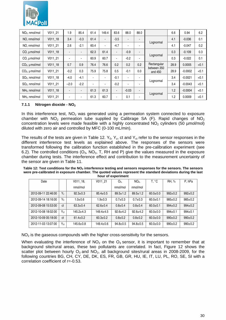
The results of the tests are given in Table 12. Y0, Yz, ct and Yct refer to the sensor responses in the different interference test levels as explained above. The responses of the sensors were transformed following the calibration function established in the pre-calibration experiment (see 6.2). The controlled conditions (O3, NO2, T, RH and P) give the values measured in the exposure chamber during tests. The interference effect and contribution to the measurement uncertainty of the sensor are given in Table 11.
Table 12: Test conditions for the NO 2 interference testing and sensors responses for the sensors. The sensors were pre-calibrated in exposure chamber. The quoted values represent the standard deviations during th e last
hour of experiment
Date V011_18,
nmol/mol
V011_21 O3,
nmol/mol
NO2,
nmol/mol
T, °C RH, % P, hPa
2012-09-11 22:46:00 Yz 92.3±0.3 85.4±0.5 89.5±1.2 89.5±1.2 60.0±0.0 992±0.2 992±0.2
2012-09-14 18:16:00 Y0 1.0±0.6 1.9±0.3 0.7±0.3 0.7±0.3 60.0±0.1 985±0.2 985±0.2
2012-09-08 15:53:00 ct 63.3±0.4 62.6±0.4 0.8±0.4 0.8±0.4 60.0±0.1 994±0.2 994±0.2
2012-10-08 18:02:00 Yct 145.2±4.3 149.4±4.5 92.6±4.2 92.6±4.2 60.0±0.0 994±0.1 994±0.1
2012-10-09 05:18:00 ct 61.4±0.2 60.3±0.2 0.8±0.2 0.8±0.2 60.0±0.0 990±0.2 990±0.2
2012-11-03 13:07:00 Yct 145.6±0.8 149.4±0.6 94.8±0.5 94.8±0.5 60.0±0.0 990±0.2 990±0.2
NO2 is the gaseous compounds with the higher cross-sensitivity for the sensors.
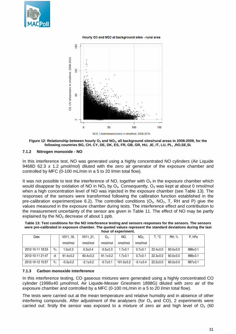
When evaluating the interference of NO2 on the O3 sensor, it is important to remember that at background site/rural areas, these two pollutants are correlated. In fact, Figure 12 shows the scatter plot between hourly O3 and NO2, all background sites/rural areas in 2008-2009, for the following countries BG, CH, CY, DE, DK, ES, FR, GB, GR, HU, IE, IT, LU, PL, RO, SE, SI with a correlation coefficient of r=-0.53.
31
Figure 12: Relationship between hourly O 3 and NO2, all background sites/rural areas in 2008-2009, fo r the
following countries BG, CH, CY, DE, DK, ES, FR, GB, GR, HU, ,IE, IT, LU, PL, ,RO,SE,SI.
7.1.2 Nitrogen monoxide - NO
In this interference test, NO was generated using a highly concentrated NO cylinders (Air Liquide 9468D 62.3 ± 1.2 µmol/mol) diluted with the zero air generator of the exposure chamber and controlled by MFC (0-100 mL/min in a 5 to 20 l/min total flow).
It was not possible to test the interference of NO, together with O3 in the exposure chamber which would disappear by oxidation of NO in NO2 by O3. Consequently, O3 was kept at about 0 nmol/mol when a high concentration level of NO was injected in the exposure chamber (see Table 13). The responses of the sensors were transformed following the calibration function established in the pre-calibration experiment(see 6.2). The controlled conditions (O3, NO2, T, RH and P) give the values measured in the exposure chamber during tests. The interference effect and contribution to the measurement uncertainty of the sensor are given in Table 11. The effect of NO may be partly explained by the NO2 decrease of about 1 ppb.
Table 13: Test conditions for the NO interference t esting and sensors responses for the sensors. The s ensors were pre-calibrated in exposure chamber. The quoted values represent the standard deviations during th e last
hour of experiment.
Date V011_18,
nmol/mol
V011_21,
nmol/mol
O3,
nmol/mol
NO,
nmol/mol
NO2,
nmol/mol
T, °C RH, % P, hPa
2012-10-11 18:53 Y0 1.0±0.3 0.3±0.4 -0.5±0.3 1.7±0.1 0.7±0.1 22.4±0.0 60.0±0.0 988±0.1
2012-10-11 21:47 ct 61.4±0.2 60.4±0.2 61.1±0.2 1.7±0.1 0.7±0.1 22.3±0.0 60.0±0.0 988±0.1
2012-10-12 15:57 Yz -0.3±0.2 -2.1±0.2 -0.7±0.1 101.0±0.2 -0.1±0.4 22.2±0.0 60.0±0.0 987±0.1
7.1.3 Carbon monoxide interference
In this interference testing, CO gaseous mixtures were generated using a highly concentrated CO cylinder (1998±40 µmol/mol, Air Liquide-Messer Grieshiem 1898G) diluted with zero air of the exposure chamber and controlled by a MFC (0-100 mL/min in a 5 to 20 l/min total flow).
The tests were carried out at the mean temperature and relative humidity and in absence of other interfering compounds. After adjustment of the analysers (for O3 and CO), 2 experiments were carried out: firstly the sensor was exposed to a mixture of zero air and high level of O3 (60
O3,
UV
pho
tom
etry
in n
mol
/mol
, 200
8-20
10
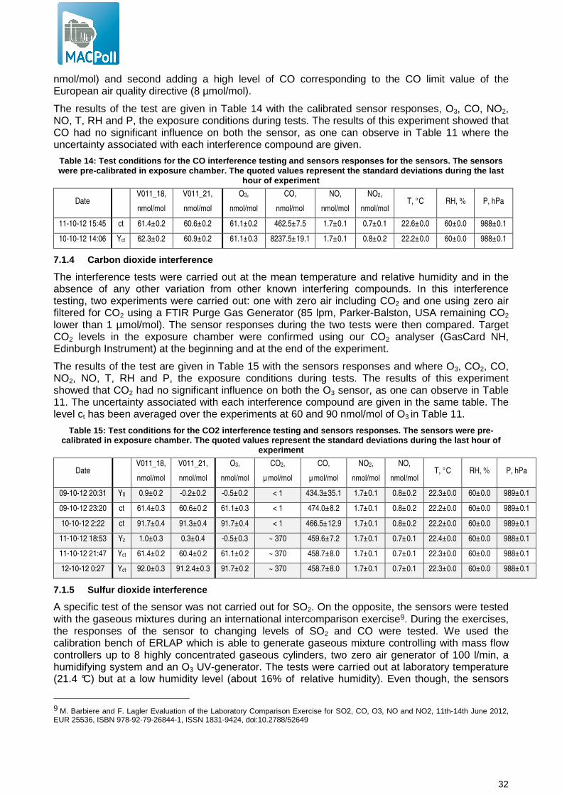
32
nmol/mol) and second adding a high level of CO corresponding to the CO limit value of the European air quality directive (8 µmol/mol).
The results of the test are given in Table 14 with the calibrated sensor responses, O3, CO, NO2, NO, T, RH and P, the exposure conditions during tests. The results of this experiment showed that CO had no significant influence on both the sensor, as one can observe in Table 11 where the uncertainty associated with each interference compound are given.
Table 14: Test conditions for the CO interference t esting and sensors responses for the sensors. The s ensors were pre-calibrated in exposure chamber. The quoted values represent the standard deviations during th e last
hour of experiment
Date V011_18,
nmol/mol
V011_21,
nmol/mol
O3,
nmol/mol
CO,
nmol/mol
NO,
nmol/mol
NO2,
nmol/mol T, °C RH, % P, hPa
11-10-12 15:45 ct 61.4±0.2 60.6±0.2 61.1±0.2 462.5±7.5 1.7±0.1 0.7±0.1 22.6±0.0 60±0.0 988±0.1
10-10-12 14:06 Yct 62.3±0.2 60.9±0.2 61.1±0.3 8237.5±19.1 1.7±0.1 0.8±0.2 22.2±0.0 60±0.0 988±0.1
7.1.4 Carbon dioxide interference
The interference tests were carried out at the mean temperature and relative humidity and in the absence of any other variation from other known interfering compounds. In this interference testing, two experiments were carried out: one with zero air including CO2 and one using zero air filtered for CO2 using a FTIR Purge Gas Generator (85 lpm, Parker-Balston, USA remaining CO2 lower than 1 µmol/mol). The sensor responses during the two tests were then compared. Target CO2 levels in the exposure chamber were confirmed using our CO2 analyser (GasCard NH, Edinburgh Instrument) at the beginning and at the end of the experiment.
The results of the test are given in Table 15 with the sensors responses and where O3, CO2, CO, NO2, NO, T, RH and P, the exposure conditions during tests. The results of this experiment showed that CO2 had no significant influence on both the O3 sensor, as one can observe in Table 11. The uncertainty associated with each interference compound are given in the same table. The level ct has been averaged over the experiments at 60 and 90 nmol/mol of O3 in Table 11.
Table 15: Test conditions for the CO2 interference testing and sensors responses. The sensors were pre -calibrated in exposure chamber. The quoted values r epresent the standard deviations during the last ho ur of
experiment
Date V011_18,
nmol/mol
V011_21,
nmol/mol
O3,
nmol/mol
CO2,
µ mol/mol
CO,
µ mol/mol
NO2,
nmol/mol
NO,
nmol/mol T, °C RH, % P, hPa
09-10-12 20:31 Y0 0.9±0.2 -0.2±0.2 -0.5±0.2 < 1 434.3±35.1 1.7±0.1 0.8±0.2 22.3±0.0 60±0.0 989±0.1
09-10-12 23:20 ct 61.4±0.3 60.6±0.2 61.1±0.3 < 1 474.0±8.2 1.7±0.1 0.8±0.2 22.2±0.0 60±0.0 989±0.1
10-10-12 2:22 ct 91.7±0.4 91.3±0.4 91.7±0.4 < 1 466.5±12.9 1.7±0.1 0.8±0.2 22.2±0.0 60±0.0 989±0.1
11-10-12 18:53 Yz 1.0±0.3 0.3±0.4 -0.5±0.3 ~ 370 459.6±7.2 1.7±0.1 0.7±0.1 22.4±0.0 60±0.0 988±0.1
11-10-12 21:47 Yct 61.4±0.2 60.4±0.2 61.1±0.2 ~ 370 458.7±8.0 1.7±0.1 0.7±0.1 22.3±0.0 60±0.0 988±0.1
12-10-12 0:27 Yct 92.0±0.3 91.2.4±0.3 91.7±0.2 ~ 370 458.7±8.0 1.7±0.1 0.7±0.1 22.3±0.0 60±0.0 988±0.1
7.1.5 Sulfur dioxide interference
A specific test of the sensor was not carried out for SO2. On the opposite, the sensors were tested with the gaseous mixtures during an international intercomparison exercise9. During the exercises, the responses of the sensor to changing levels of SO2 and CO were tested. We used the calibration bench of ERLAP which is able to generate gaseous mixture controlling with mass flow controllers up to 8 highly concentrated gaseous cylinders, two zero air generator of 100 l/min, a humidifying system and an O3 UV-generator. The tests were carried out at laboratory temperature (21.4 °C) but at a low humidity level (about 16% of relative humidity). Even though, the sensors
9 M. Barbiere and F. Lagler Evaluation of the Laboratory Comparison Exercise for SO2, CO, O3, NO and NO2, 11th-14th June 2012, EUR 25536, ISBN 978-92-79-26844-1, ISSN 1831-9424, doi:10.2788/52649
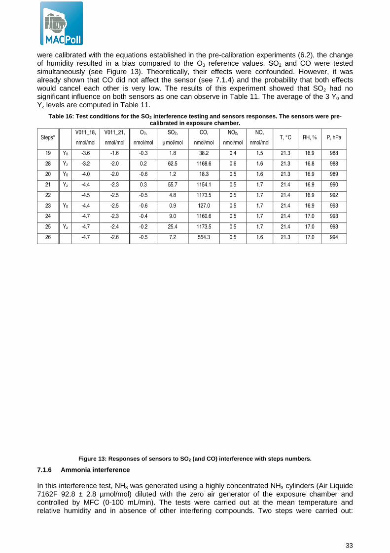
were calibrated with the equations established in the preof humidity resulted in a bias compared to the Osimultaneously (see Figure 13). Theoretically, their effects were confounded. However, it was already shown that CO did not affect the sensor (see would cancel each other is very low. The results of this experiment showed that SOsignificant influence on both sensors as one can observe in Yz levels are computed in Table 11
Table 16: Test conditions for the SO
Steps° V011_18,
nmol/mol
V011_21,
nmol/mol
O
nmol/mol
19 Y0 -3.6 -1.6 -0.3
28 Yz -3.2 -2.0 0.2
20 Y0 -4.0 -2.0 -0.6
21 Yz -4.4 -2.3 0.3
22 -4.5 -2.5 -0.5
23 Y0 -4.4 -2.5 -0.6
24 -4.7 -2.3 -0.4
25 Yz -4.7 -2.4 -0.2
26 -4.7 -2.6 -0.5
Figure 13 : Responses of sensors to SO
7.1.6 Ammonia interference
In this interference test, NH3 was generated using a highly concentrated NH7162F 92.8 ± 2.8 µmol/mol) diluted with the zero air generator of the exposure chamber and controlled by MFC (0-100 mL/min). The tests were carried out at the mean temperature and relative humidity and in absence of other interferin
were calibrated with the equations established in the pre-calibration experiments (of humidity resulted in a bias compared to the O3 reference values. SO2
). Theoretically, their effects were confounded. However, it was already shown that CO did not affect the sensor (see 7.1.4) and the probability that both effects would cancel each other is very low. The results of this experiment showed that SOsignificant influence on both sensors as one can observe in Table 11. The average of the 3 Y
11.
: Test conditions for the SO 2 interference testing and sensors responses. The sen sors were precalibrated in exposure chamber.
O3,
nmol/mol
SO2,
µ mol/mol
CO,
nmol/mol
NO2,
nmol/mol
NO,
nmol/mol T, °C
0.3 1.8 38.2 0.4 1.5 21.3
0.2 62.5 1168.6 0.6 1.6 21.3
0.6 1.2 18.3 0.5 1.6 21.3
0.3 55.7 1154.1 0.5 1.7 21.4
0.5 4.8 1173.5 0.5 1.7 21.4
0.6 0.9 127.0 0.5 1.7 21.4
0.4 9.0 1160.6 0.5 1.7 21.4
0.2 25.4 1173.5 0.5 1.7 21.4
0.5 7.2 554.3 0.5 1.6 21.3
: Responses of sensors to SO 2 (and CO) interference with steps numbers.
was generated using a highly concentrated NH3
7162F 92.8 ± 2.8 µmol/mol) diluted with the zero air generator of the exposure chamber and 100 mL/min). The tests were carried out at the mean temperature and
relative humidity and in absence of other interfering compounds. Two steps were carried out:
33
calibration experiments (6.2), the change and CO were tested
). Theoretically, their effects were confounded. However, it was ) and the probability that both effects
would cancel each other is very low. The results of this experiment showed that SO2 had no . The average of the 3 Y0 and
interference testing and sensors responses. The sen sors were pre -
T, °C RH, % P, hPa
21.3 16.9 988
21.3 16.8 988
21.3 16.9 989
21.4 16.9 990
21.4 16.9 992
21.4 16.9 993
21.4 17.0 993
21.4 17.0 993
21.3 17.0 994
(and CO) interference with steps numbers.
3 cylinders (Air Liquide 7162F 92.8 ± 2.8 µmol/mol) diluted with the zero air generator of the exposure chamber and
100 mL/min). The tests were carried out at the mean temperature and g compounds. Two steps were carried out:
34
firstly, the sensor was exposed to a mixture of zero air and O3 (ct = 60 nmol/mol) and second adding a high level of NH3.
The results of the test are given in Table 17 with the calibrated sensors responses and where O3, CO, NO2, NO, T, RH and P gives the values of the conditions in the exposure during tests. The results of this experiment showed that NH3 has no significant influence on both the Sensors as one can observe in Table 11 where the uncertainty associated with each interference compound is given.
Table 17: Test conditions for the NH3 interference testing and sensors responses for the sensors. The sensors were pre-calibrated in exposure chamber. The quoted values represent the standard deviations during th e last
hour of experiment.
Date V011_18,
nmol/mol
V011_21,
nmol/mol
O3,
nmol/mol
NH3,
nmol/mol
CO,
µ mol/mol
NO,
nmol/mol
NO2,
nmol/mol T, °C RH, % P, hPa
11-10-12 14:40 ct 61.4±0.1 60.7±0.1 61.1±0.2 0 463.7±7.5 1.7±0.1 0.8±0.1 22.7±0.0 60±0.0 988±0.2
11-10-12 15:45 Yct 61.4±0.2 60.6±0.2 61.1±0.2 85 462.5±7.5 1.7±0.1 0.7±0.1 22.6±0.0 60±0.0 988±0.1
7.2 Air Matrix
The effect of air matrix on the sensor response was tested at all the O3 levels of the pre-calibration experiment (see 6.2). Three different air matrixes were tested: zero air (filtered air), ambient air added to zero air and indoor air added to zero air.
During the experiment, all parameters suspected to have an effect on the sensor response (test gas, temperature, humidity test values and other possible influencing) were kept under strict control with relative standard deviation of about 1.5 % as shown in Table 18.
For zero air, the generator of the ERLAP calibration bench (see 5.2) was used. For the two other experiments, a constant air flow, 16.7 l/min, of ambient air and indoor air was injected in the exposure chamber together with zero air.
A low volume sampler (LVS, Derenda 3.1 samplers - G) was used to draw samples from bulk air. Particulate matter was removed from the bulk air using a European PM10 sampling head (EN 12341). The air was sampled just outside our laboratory (nearby a small parking lot) for ambient air and inside our laboratory for the indoor air experiment. The LVS sampling inlets was cleaned before sampling without being greased as requested in EN 12341. The sampling flow of the LVS was adjusted to 1 m³/hr. The target O3 levels and relative humidity was reached by continuous automatic adjustment of the flows of zero air (dry and humid flows, see the air generator 5.2) before being mixed with the ambient or indoor air constant flow. Therefore the total flow of zero air was different at each experiment. They ranged between 4 and 20 l/min.
A low NO2 value was measured during the sampling with ambient and indoor. Since NO2 was found to be an interfering compound (see 7.1.1), the sensor responses were plotted against the sum of O3 and NO2 levels multiplied by the percentage of NO2 interference on the sensor. Figure 14 presents the sensor responses for the different air matrixes with the NO2 interference taken into account. Three calibration curves were plotted, one only using zero air for dilution, one using a mixture of ambient and zero air and one using a mixture of indoor and ambient air. The sensor responses show negligible matrix effect. These results do not give evidence of any important effect that was not tested in the interference paragraphs.
ccbaRs ⋅+= Eq. 16
b
aRscr
−=
Eq. 17
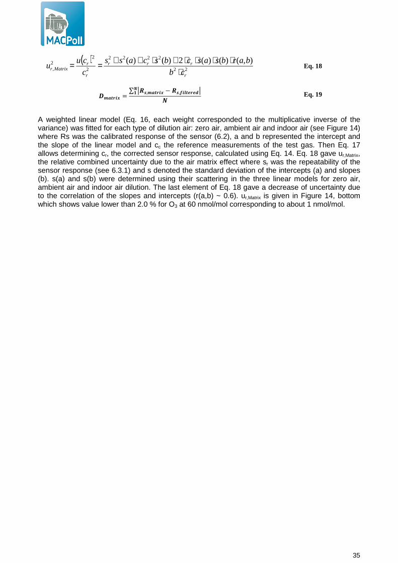
35
( )22
2222
2
22,
),()()(2)()(
r
rrr
r
rMatrixr cb
barbsascbscass
c
cuu
⋅⋅⋅⋅⋅+⋅++== Eq. 18
#)���*+ =∑ %&�,)���*+ − &�,�*,����-%!� ' Eq. 19
A weighted linear model (Eq. 16, each weight corresponded to the multiplicative inverse of the variance) was fitted for each type of dilution air: zero air, ambient air and indoor air (see Figure 14) where Rs was the calibrated response of the sensor (6.2), a and b represented the intercept and the slope of the linear model and cc the reference measurements of the test gas. Then Eq. 17 allows determining cr, the corrected sensor response, calculated using Eq. 14. Eq. 18 gave ur,Matrix, the relative combined uncertainty due to the air matrix effect where sr was the repeatability of the sensor response (see 6.3.1) and s denoted the standard deviation of the intercepts (a) and slopes (b). s(a) and s(b) were determined using their scattering in the three linear models for zero air, ambient air and indoor air dilution. The last element of Eq. 18 gave a decrease of uncertainty due to the correlation of the slopes and intercepts (r(a,b) ~ 0.6). ur,Matrix is given in Figure 14, bottom which shows value lower than 2.0 % for O3 at 60 nmol/mol corresponding to about 1 nmol/mol.
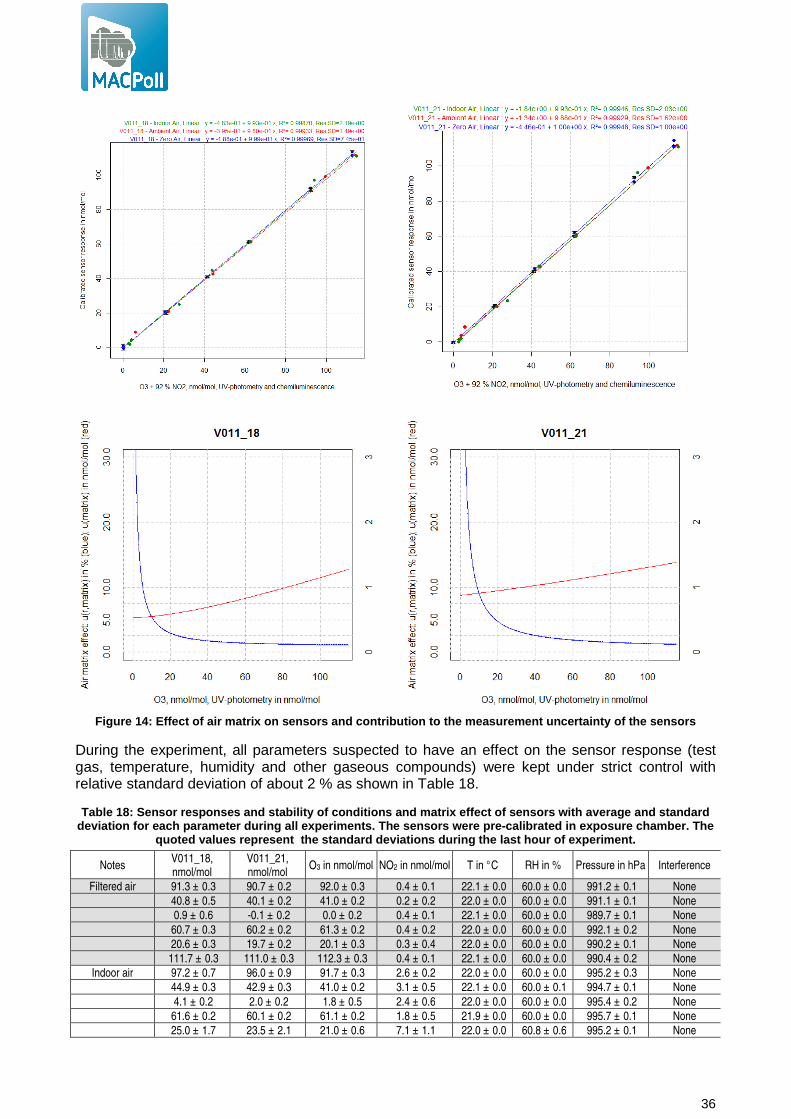
36
Figure 14: Effect of air matrix on sensors and contr ibution to the measurement uncertainty of the senso rs
During the experiment, all parameters suspected to have an effect on the sensor response (test gas, temperature, humidity and other gaseous compounds) were kept under strict control with relative standard deviation of about 2 % as shown in Table 18.
Table 18: Sensor responses and stability of conditio ns and matrix effect of sensors with average and st andard deviation for each parameter during all experiments . The sensors were pre-calibrated in exposure chamb er. The
quoted values represent the standard deviations du ring the last hour of experiment.
Notes V011_18, nmol/mol
V011_21, nmol/mol
O3 in nmol/mol NO2 in nmol/mol T in °C RH in % Pressure in hPa Interference
Filtered air 91.3 ± 0.3 90.7 ± 0.2 92.0 ± 0.3 0.4 ± 0.1 22.1 ± 0.0 60.0 ± 0.0 991.2 ± 0.1 None
40.8 ± 0.5 40.1 ± 0.2 41.0 ± 0.2 0.2 ± 0.2 22.0 ± 0.0 60.0 ± 0.0 991.1 ± 0.1 None
0.9 ± 0.6 -0.1 ± 0.2 0.0 ± 0.2 0.4 ± 0.1 22.1 ± 0.0 60.0 ± 0.0 989.7 ± 0.1 None
60.7 ± 0.3 60.2 ± 0.2 61.3 ± 0.2 0.4 ± 0.2 22.0 ± 0.0 60.0 ± 0.0 992.1 ± 0.2 None
20.6 ± 0.3 19.7 ± 0.2 20.1 ± 0.3 0.3 ± 0.4 22.0 ± 0.0 60.0 ± 0.0 990.2 ± 0.1 None
111.7 ± 0.3 111.0 ± 0.3 112.3 ± 0.3 0.4 ± 0.1 22.1 ± 0.0 60.0 ± 0.0 990.4 ± 0.2 None
Indoor air 97.2 ± 0.7 96.0 ± 0.9 91.7 ± 0.3 2.6 ± 0.2 22.0 ± 0.0 60.0 ± 0.0 995.2 ± 0.3 None
44.9 ± 0.3 42.9 ± 0.3 41.0 ± 0.2 3.1 ± 0.5 22.1 ± 0.0 60.0 ± 0.1 994.7 ± 0.1 None
4.1 ± 0.2 2.0 ± 0.2 1.8 ± 0.5 2.4 ± 0.6 22.0 ± 0.0 60.0 ± 0.0 995.4 ± 0.2 None
61.6 ± 0.2 60.1 ± 0.2 61.1 ± 0.2 1.8 ± 0.5 21.9 ± 0.0 60.0 ± 0.0 995.7 ± 0.1 None
25.0 ± 1.7 23.5 ± 2.1 21.0 ± 0.6 7.1 ± 1.1 22.0 ± 0.0 60.8 ± 0.6 995.2 ± 0.1 None
37
111.1 ± 0.5 110.7 ± 0.7 112.0 ± 0.3 3.2 ± 0.5 22.0 ± 0.0 60.0 ± 0.0 994.5 ± 0.2 None
Outdoor air 99.0 ± 0.6 98.9 ± 0.7 91.8 ± 0.5 8.3 ± 0.6 22.6 ± 0.0 60.0 ± 0.1 997.6 ± 0.1 None
42.6 ± 0.6 42.6 ± 0.7 41.0 ± 0.2 3.6 ± 0.6 22.5 ± 0.0 59.9 ± 0.1 998.5 ± 0.1 None
4.6 ± 0.8 3.6 ± 1.0 1.8 ± 0.3 2.5 ± 0.5 22.3 ± 0.0 59.6 ± 0.2 995.7 ± 0.1 None
61.1 ± 0.2 60.7 ± 0.2 61.1 ± 0.3 1.9 ± 0.7 22.3 ± 0.0 60.0 ± 0.0 995.9 ± 0.1 None
21.0 ± 0.3 20.1 ± 0.2 19.8 ± 0.3 2.8 ± 0.5 22.3 ± 0.0 60.0 ± 0.0 995.2 ± 0.1 None
111.7 ± 0.2 111.6 ± 0.2 112.1 ± 0.2 2.5 ± 0.5 22.2 ± 0.0 60.0 ± 0.0 993.8 ± 0.2 None
7.3 Hysteresis
Hysteresis is the dependence of a system not only on its current environment but also on its past environment. This dependence arises because the system can be in more than one internal state. To predict its future development, either its internal state or its history must be known. If a given input alternately increases and decreases, the output tends to form a loop.
The estimation of the dependence of sensors toward hysteresis was carried out by testing a ramp of rising O3 levels (0, 20, 40, 60, 80, 95% of FS), followed with a ramp of decreasing level and finally with a rising ramp as shown in Table 19. Each point corresponds to the hourly average for one O3 concentration at the mean temperature and mean relative humidity.
Table 19: Sensor responses and stability of conditio ns during the experiments for the determination of hysteresis effect. The sensors were pre-calibrated in exposure chamber. The quoted values represent th e
standard deviations during the last hour of experim ent.
Notes V011_18, nmol/mol
V011_21, nmol/mol
O3 in nmol/mol NO2 in nmol/mol T in °C RH in % Pressure in
hPa
Rise -3.0 ± 0.7 -2.1 ± 0.3 -0.5 ± 0.2 0.4 ± 0.1 22.0 ± 0.0 60.0 ± 0.0 989.2 ± 0.2
18.8 ± 0.5 19.0 ± 0.3 20.1 ± 0.3 0.4 ± 0.1 22.0 ± 0.0 60.0 ± 0.0 990.9 ± 0.1
39.6 ± 0.4 39.6 ± 0.3 40.7 ± 0.3 0.4 ± 0.3 22.0 ± 0.0 60.0 ± 0.0 991.2 ± 0.1
60.1 ± 0.3 60.0 ± 0.2 61.3 ± 0.2 0.4 ± 0.4 22.0 ± 0.0 60.0 ± 0.0 991.3 ± 0.1
90.9 ± 0.3 90.6 ± 0.2 91.9 ± 0.2 0.2 ± 0.3 22.0 ± 0.0 60.0 ± 0.0 992.1 ± 0.2
111.3 ± 0.3 111.0 ± 0.3 112.4 ± 0.3 0.4 ± 0.2 22.1 ± 0.0 60.0 ± 0.1 992.2 ± 0.1
Fall 91.6 ± 0.2 91.1 ± 0.2 91.9 ± 0.3 0.4 ± 0.2 22.0 ± 0.0 60.0 ± 0.0 991.1 ± 0.2
61.9 ± 0.4 60.7 ± 0.2 61.3 ± 0.2 0.4 ± 0.1 22.0 ± 0.0 60.0 ± 0.0 989.6 ± 0.2
41.5 ± 0.4 40.6 ± 0.3 41.0 ± 0.4 0.4 ± 0.1 22.0 ± 0.0 60.0 ± 0.1 989.0 ± 0.1
21.1 ± 0.5 20.0 ± 0.3 20.3 ± 0.3 0.4 ± 0.2 22.0 ± 0.0 60.0 ± 0.1 989.9 ± 0.1
0.8 ± 0.5 -0.5 ± 0.2 -0.4 ± 0.2 0.3 ± 0.2 22.0 ± 0.0 60.0 ± 0.0 990.2 ± 0.1
Rise 20.6 ± 0.3 19.7 ± 0.2 20.1 ± 0.3 0.3 ± 0.4 22.0 ± 0.0 60.0 ± 0.0 990.2 ± 0.1
40.8 ± 0.5 40.1 ± 0.2 41.0 ± 0.2 0.2 ± 0.2 22.0 ± 0.0 60.0 ± 0.0 991.1 ± 0.1
60.7 ± 0.3 60.2 ± 0.2 61.3 ± 0.2 0.4 ± 0.2 22.0 ± 0.0 60.0 ± 0.0 992.1 ± 0.2
91.3 ± 0.3 90.7 ± 0.2 92.0 ± 0.3 0.4 ± 0.1 22.1 ± 0.0 60.0 ± 0.0 991.2 ± 0.1
111.7 ± 0.3 111.0 ± 0.3 112.3 ± 0.3 0.4 ± 0.1 22.1 ± 0.0 60.0 ± 0.0 990.4 ± 0.2
Figure 15 presents the sensor responses. Three curves are plotted, one for the 1st ramp of rising O3 levels, one for the 2nd one with falling levels and one for the 3rd ramp of rising levels. The sensors shows nearly no hysteresis effect with a slight change of the intercept of linear equations for the 1st sensor.
In the same manner as in 7.2, a weighted linear line was fitted for each ramp of O3 levels (see Figure 15). ur,h, the relative combined uncertainty due to the hysteresis effect was calculated using Eq. 18 where sr was the repeatability of the sensor response (evaluated in 6.3.1) and s denoted the standard deviation of the slopes (b) and intercepts (a). s(a) and s(b) were determined using their scattering in the linear lines of each ramp of O3 concentration levels. The correlation between the slopes and intercepts in Eq. 18 was not significant. The relative standard uncertainty due to hysteresis effect, ur,h, is given in Figure 15, bottom and shows value lower than 0.2 % for O3 higher than 10 nmol/mol corresponding to about 1 nmol/mol at O3 concentration level of 120 nmol/mol.
38
Figure 15: Effect of hysteresis on sensors and contr ibution of the hysteresis effect to the measurement
uncertainty
7.4 Meteorological parameters
7.4.1 Temperature and humidity
Sensor’s response can also be influenced by changes of temperature or relative humidity. To evaluate these effects, we carried out two series of test, generating ramps of temperature or humidity while O3 and other significant parameters (the sole NO2) remained under strict control see Figure 17 and Table 20. The ranges of temperature changed between 12 and 32 ºC (by step of 5 ºC) and the range of humidity was kept between 40% and 80% (by step of 10%), as shown on Figure 16.
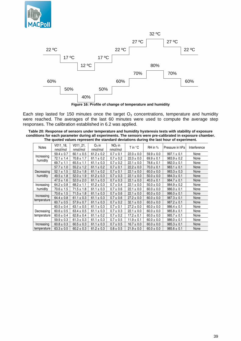
39
32 ºC
27 ºC 27 ºC
22 ºC 22 ºC 22 ºC
17 ºC 17 ºC
12 ºC 80%
70% 70%
60% 60% 60%
50% 50%
40%
Figure 16: Profile of change of temperature and humi dity
Each step lasted for 150 minutes once the target O3 concentrations, temperature and humidity were reached. The averages of the last 60 minutes were used to compute the average step responses. The calibration established in 6.2 was applied.
Table 20: Response of sensors under temperature and humidity hysteresis tests with stability of exposu re conditions for each parameter during all experiment s. The sensors were pre-calibrated in exposure cham ber.
The quoted values represent the standard deviations during the last hour of experiment.
Notes V011_18, nmol/mol
V011_21, nmol/mol
O3 in nmol/mol
NO2 in nmol/mol
T in °C RH in % Pressure in hPa Interference
Increasing humidity
59.4 ± 0.7 60.1 ± 0.5 61.2 ± 0.2 0.7 ± 0.1 22.0 ± 0.0 59.9 ± 0.0 997.1 ± 0.1 None
72.1 ± 1.4 70.8 ± 1.7 61.1 ± 0.2 0.7 ± 0.2 22.0 ± 0.0 69.9 ± 0.1 983.9 ± 0.2 None
69.7 ± 1.1 65.5 ± 1.1 61.1 ± 0.3 0.7 ± 0.2 22.1 ± 0.0 78.6 ± 0.1 982.0 ± 0.1 None
Decreasing humidity
57.7 ± 1.0 55.2 ± 1.2 61.1 ± 0.2 0.7 ± 0.1 22.2 ± 0.0 70.0 ± 0.1 983.1 ± 0.1 None
52.1 ± 1.5 52.3 ± 1.8 61.1 ± 0.2 0.7 ± 0.1 22.1 ± 0.0 60.0 ± 0.0 983.3 ± 0.3 None
49.5 ± 1.8 52.0 ± 1.9 61.2 ± 0.3 0.7 ± 0.3 22.1 ± 0.0 50.0 ± 0.0 984.3 ± 0.1 None
47.5 ± 1.6 52.0 ± 2.0 61.1 ± 0.3 0.7 ± 0.3 22.1 ± 0.0 40.0 ± 0.1 984.7 ± 0.1 None
Increasing humidity
64.2 ± 0.8 68.2 ± 1.1 61.2 ± 0.3 0.7 ± 0.4 22.1 ± 0.0 50.0 ± 0.0 984.9 ± 0.2 None
70.6 ± 1.5 71.5 ± 1.8 61.1 ± 0.3 0.7 ± 0.6 22.1 ± 0.0 60.0 ± 0.0 986.0 ± 0.1 None
Increasing temperature
70.6 ± 1.5 71.5 ± 1.8 61.1 ± 0.3 0.7 ± 0.6 22.1 ± 0.0 60.0 ± 0.0 986.0 ± 0.1 None
64.4 ± 0.8 61.1 ± 0.3 61.1 ± 0.3 0.7 ± 0.6 27.2 ± 0.0 60.0 ± 0.0 987.3 ± 0.1 None
60.7 ± 0.5 57.9 ± 0.7 61.1 ± 0.3 0.7 ± 0.2 32.1 ± 0.0 60.0 ± 0.0 987.2 ± 0.1 None
Decreasing temperature
60.5 ± 0.4 63.1 ± 0.5 61.1 ± 0.3 0.7 ± 0.1 27.2 ± 0.0 60.0 ± 0.0 986.4 ± 0.1 None
60.6 ± 0.5 63.4 ± 0.5 61.1 ± 0.3 0.7 ± 0.3 22.1 ± 0.0 60.0 ± 0.0 985.8 ± 0.1 None
60.6 ± 0.4 62.8 ± 0.4 61.1 ± 0.2 0.7 ± 0.2 17.2 ± 0.1 60.0 ± 0.0 985.7 ± 0.1 None
59.9 ± 0.3 61.3 ± 0.3 61.1 ± 0.3 0.7 ± 0.5 11.9 ± 0.1 60.0 ± 0.0 986.0 ± 0.1 None
Increasing temperature
60.8 ± 0.3 60.5 ± 0.3 61.1 ± 0.3 0.7 ± 0.5 16.7 ± 0.0 60.0 ± 0.0 985.3 ± 0.1 None
63.3 ± 0.5 60.2 ± 0.3 61.2 ± 0.3 0.8 ± 0.5 21.9 ± 0.0 60.0 ± 0.0 985.6 ± 0.1 None
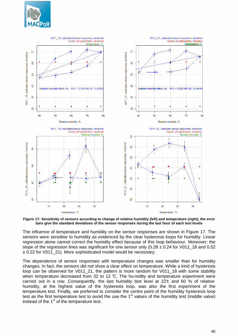
40
Figure 17: Sensitivity of sensors according to chang e of relative humidity (left) and temperature (righ t), the error
bars give the standard deviations of the sensor res ponses during the last hour of each test levels
The influence of temperature and humidity on the sensor responses are shown in Figure 17. The sensors were sensitive to humidity as evidenced by the clear hysteresis loops for humidity. Linear regression alone cannot correct the humidity effect because of this loop behaviour. Moreover; the slope of the regression lines was significant for one sensor only (0.28 ± 0.24 for V011_18 and 0.52 ± 0.22 for V011_21). More sophisticated model would be necessary.
The dependence of sensor responses with temperature changes was smaller than for humidity changes. In fact, the sensors did not show a clear effect on temperature. While a kind of hysteresis loop can be observed for V011_21, the pattern is more random for V011_18 with some stability when temperature decreased from 32 to 12 °C. The hu midity and temperature experiment were carried out in a row. Consequently, the last humidity test level at 22°c and 60 % of relative humidity, at the highest value of the hysteresis loop, was also the first experiment of the temperature test. Finally, we preferred to consider the centre point of the humidity hysteresis loop test as the first temperature test to avoid the use the 1st values of the humidity test (middle value) instead of the 1st of the temperature test.
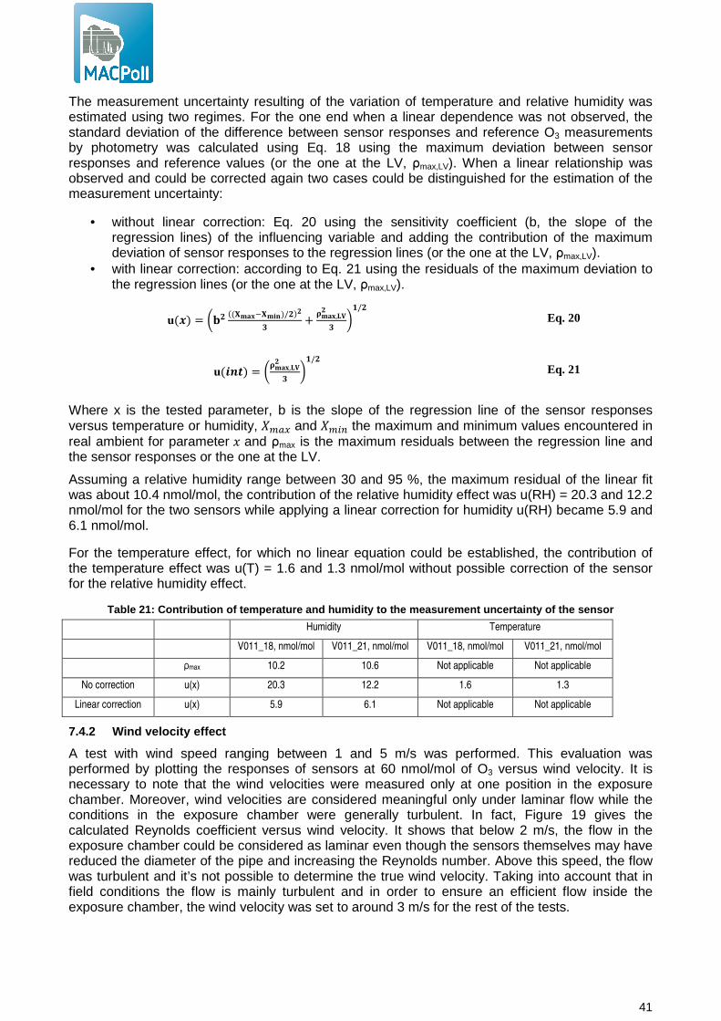
41
The measurement uncertainty resulting of the variation of temperature and relative humidity was estimated using two regimes. For the one end when a linear dependence was not observed, the standard deviation of the difference between sensor responses and reference O3 measurements by photometry was calculated using Eq. 18 using the maximum deviation between sensor responses and reference values (or the one at the LV, ρmax,LV). When a linear relationship was observed and could be corrected again two cases could be distinguished for the estimation of the measurement uncertainty:
• without linear correction: Eq. 20 using the sensitivity coefficient (b, the slope of the regression lines) of the influencing variable and adding the contribution of the maximum deviation of sensor responses to the regression lines (or the one at the LV, ρmax,LV).
• with linear correction: according to Eq. 21 using the residuals of the maximum deviation to the regression lines (or the one at the LV, ρmax,LV).
u(.) = �/� �(.���.��)/��
/+
0��,��
/��/� Eq. 20
u(012) = �0��,��
/��/� Eq. 21
Where x is the tested parameter, b is the slope of the regression line of the sensor responses versus temperature or humidity, �� and ��� the maximum and minimum values encountered in real ambient for parameter � and ρmax is the maximum residuals between the regression line and the sensor responses or the one at the LV.
Assuming a relative humidity range between 30 and 95 %, the maximum residual of the linear fit was about 10.4 nmol/mol, the contribution of the relative humidity effect was u(RH) = 20.3 and 12.2 nmol/mol for the two sensors while applying a linear correction for humidity u(RH) became 5.9 and 6.1 nmol/mol.
For the temperature effect, for which no linear equation could be established, the contribution of the temperature effect was u(T) = 1.6 and 1.3 nmol/mol without possible correction of the sensor for the relative humidity effect.
Table 21: Contribution of temperature and humidity to the measurement uncertainty of the sensor
Humidity Temperature
V011_18, nmol/mol V011_21, nmol/mol V011_18, nmol/mol V011_21, nmol/mol
ρmax 10.2 10.6 Not applicable Not applicable
No correction u(x) 20.3 12.2 1.6 1.3
Linear correction u(x) 5.9 6.1 Not applicable Not applicable
7.4.2 Wind velocity effect
A test with wind speed ranging between 1 and 5 m/s was performed. This evaluation was performed by plotting the responses of sensors at 60 nmol/mol of O3 versus wind velocity. It is necessary to note that the wind velocities were measured only at one position in the exposure chamber. Moreover, wind velocities are considered meaningful only under laminar flow while the conditions in the exposure chamber were generally turbulent. In fact, Figure 19 gives the calculated Reynolds coefficient versus wind velocity. It shows that below 2 m/s, the flow in the exposure chamber could be considered as laminar even though the sensors themselves may have reduced the diameter of the pipe and increasing the Reynolds number. Above this speed, the flow was turbulent and it’s not possible to determine the true wind velocity. Taking into account that in field conditions the flow is mainly turbulent and in order to ensure an efficient flow inside the exposure chamber, the wind velocity was set to around 3 m/s for the rest of the tests.
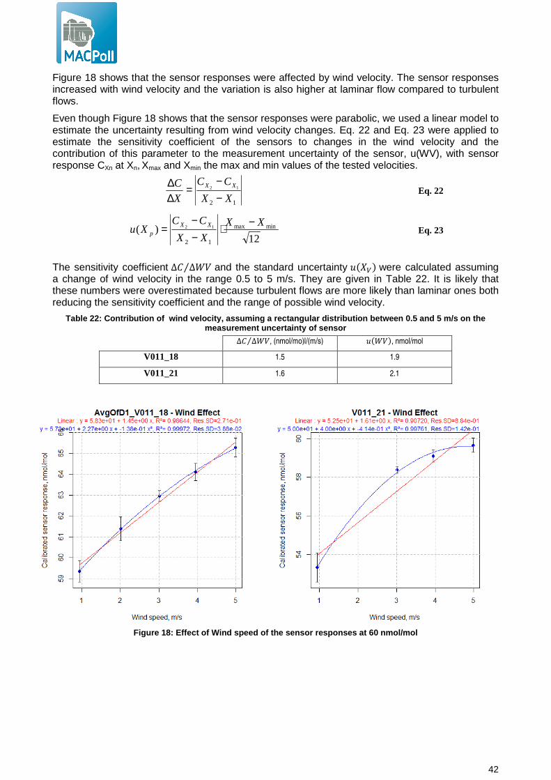
42
Figure 18 shows that the sensor responses were affected by wind velocity. The sensor responses increased with wind velocity and the variation is also higher at laminar flow compared to turbulent flows.
Even though Figure 18 shows that the sensor responses were parabolic, we used a linear model to estimate the uncertainty resulting from wind velocity changes. Eq. 22 and Eq. 23 were applied to estimate the sensitivity coefficient of the sensors to changes in the wind velocity and the contribution of this parameter to the measurement uncertainty of the sensor, u(WV), with sensor response CXn at Xn, Xmax and Xmin the max and min values of the tested velocities.
12
12
XX
CC
X
C XX
−−
=∆∆
Eq. 22
12)( minmax
12
12XX
XX
CCXu XX
p
−⋅−−
= Eq. 23
The sensitivity coefficient ∆� ∆�⁄ and the standard uncertainty ��� were calculated assuming a change of wind velocity in the range 0.5 to 5 m/s. They are given in Table 22. It is likely that these numbers were overestimated because turbulent flows are more likely than laminar ones both reducing the sensitivity coefficient and the range of possible wind velocity.
Table 22: Contribution of wind velocity, assuming a rectangular distribution between 0.5 and 5 m/s on the measurement uncertainty of sensor
∆� ∆��⁄ , (nmol/mo)l/(m/s) �����, nmol/mol
V011_18 1.5 1.9
V011_21 1.6 2.1
Figure 18: Effect of Wind speed of the sensor respon ses at 60 nmol/mol
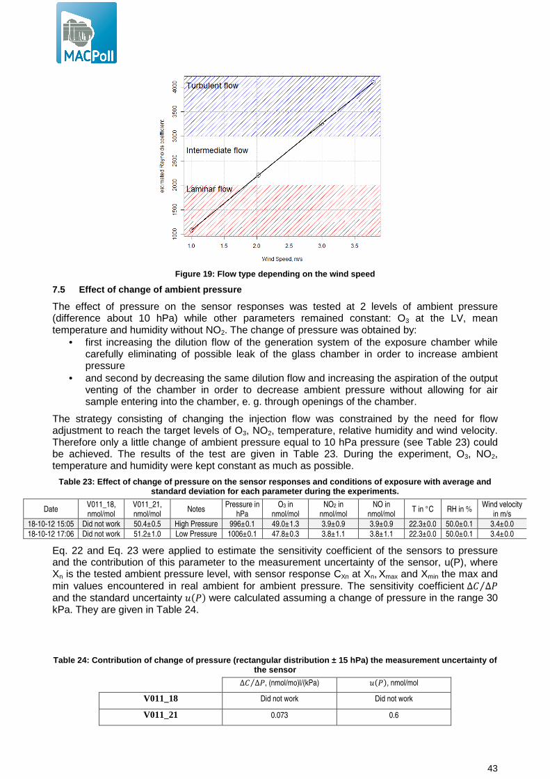
43
Figure 19: Flow type depending on the wind speed
7.5 Effect of change of ambient pressure
The effect of pressure on the sensor responses was tested at 2 levels of ambient pressure (difference about 10 hPa) while other parameters remained constant: O3 at the LV, mean temperature and humidity without NO2. The change of pressure was obtained by:
• first increasing the dilution flow of the generation system of the exposure chamber while carefully eliminating of possible leak of the glass chamber in order to increase ambient pressure
• and second by decreasing the same dilution flow and increasing the aspiration of the output venting of the chamber in order to decrease ambient pressure without allowing for air sample entering into the chamber, e. g. through openings of the chamber.
The strategy consisting of changing the injection flow was constrained by the need for flow adjustment to reach the target levels of O3, NO2, temperature, relative humidity and wind velocity. Therefore only a little change of ambient pressure equal to 10 hPa pressure (see Table 23) could be achieved. The results of the test are given in Table 23. During the experiment, O3, NO2, temperature and humidity were kept constant as much as possible.
Table 23: Effect of change of pressure on the sensor responses and conditions of exposure with average and standard deviation for each parameter during the ex periments.
Date V011_18, nmol/mol
V011_21, nmol/mol
Notes Pressure in
hPa O3 in
nmol/mol NO2 in
nmol/mol NO in
nmol/mol T in °C RH in %
Wind velocity in m/s
18-10-12 15:05 Did not work 50.4±0.5 High Pressure 996±0.1 49.0±1.3 3.9±0.9 3.9±0.9 22.3±0.0 50.0±0.1 3.4±0.0
18-10-12 17:06 Did not work 51.2±1.0 Low Pressure 1006±0.1 47.8±0.3 3.8±1.1 3.8±1.1 22.3±0.0 50.0±0.1 3.4±0.0
Eq. 22 and Eq. 23 were applied to estimate the sensitivity coefficient of the sensors to pressure and the contribution of this parameter to the measurement uncertainty of the sensor, u(P), where Xn is the tested ambient pressure level, with sensor response CXn at Xn, Xmax and Xmin the max and min values encountered in real ambient for ambient pressure. The sensitivity coefficient ∆� ∆�⁄ and the standard uncertainty ��� were calculated assuming a change of pressure in the range 30 kPa. They are given in Table 24.
Table 24: Contribution of change of pressure (recta ngular distribution ± 15 hPa) the measurement uncert ainty of the sensor
∆� ∆�⁄ , (nmol/mo)l/(kPa) ����, nmol/mol
V011_18 Did not work Did not work
V011_21 0.073 0.6
44
7.6 Effect of change in power supply
The effect of power supply on the sensor responses was tested at 3 levels of voltage (210, 220 and 230 V) while other parameters remained constant: O3 at the LV, and central point of temperature and humidity without NO2. In this experiment, a variable generator (rheostat) model Rheothor ADB was placed before the power supply of the sensor. The results of the test are given in Table 25. During the experiment, O3, NO2, temperature and humidity were kept as constant as possible.
Table 25: Effect of change of power supply on the se nsor responses and conditions of exposure with aver age and standard deviation for each parameter during th e experiments.
Date V011_18, nmol/mol
V011_21, nmol/mol
Voltage O3 in
nmol/mol NO2 in
nmol/mol T in °C RH in %
Pressure in hPa
Wind velocity in m/s
06-11-12 16:00 65.8±0.9 66.8±0.9 220 V 61.1±0.2 4.9±0.3 22.3±0.1 60.0±0.1 990.8±0.3 3.6±0.0
06-11-12 17:00 64.4±0.6 65.1±0.4 230 V 61.1±0.2 5.0±0.3 22.2±0.0 60.0±0.1 991.6±0.2 3.6±0.0
06-11-12 17:31 63.5±0.5 64.0±0.3 210 V 61.1±0.2 4.9±0.2 22.2±0.1 60.0±0.1 992.1±0.2 3.6±0.0
07-11-12 11:20 63.1±0.5 64.2±0.4 210 V 61.1±0.2 5.0±0.3 22.1±0.1 60.0±0.1 1002.7±0.1 3.7±0.0
07-11-12 13:18 63.0±0.6 64.0±0.4 230 V 61.2±0.3 5.0±0.4 22.1±0.1 60.0±0.1 1001.9±0.1 3.7±0.0
07-11-12 17:20 63.1±0.6 64.2±0.4 220 V 61.1±0.2 4.7±5.5 22.1±0.1 60.0±0.1 1002.5±0.3 3.7±0.0
Eq. 22 and Eq. 23 were applied to estimate the sensitivity coefficient of the sensors to change in the power supply and the contribution of this parameter to the measurement uncertainty of the sensor, u(V), where Xn is the tested voltage, with sensor response CXn at Xn, Xmax and Xmin the max and min values.
The sensitivity coefficient ∆� ∆⁄ and the standard uncertainty �� were calculated assuming a change of voltage between 210 and 230 V. They are given in Table 26. No effect could be evidenced. One has to remember that we used an accurate power supply model ISO-TECH IPS 303A. With this power supply it is likely that any change in voltage would be eliminated. In conclusion, it may be necessary to use a sophisticated power supply to reproduce these results.
Table 26: Contribution of power supply, assuming a rectangular distribution between 210 and 230 V, to t he measurement uncertainty of sensor
∆� ∆�⁄ , (nmol/mo)l/(V) ����, nmol/mol
V011_18 0.020 0.1
V011_21 0.023 0.1
7.7 Choice of tested interfering parameters in full factorial design
The major cross sensitivities showed by the sensors were in order of magnitude: humidity and NO2 both of them needing correction, long term drift and wind velocity, and to a minor extent: hysteresis, temperature and matrix effect. Other parameters had no or little influence: CO/CO2, NH3, SO2, matrix effect, pressure and power supply (see Table 27). Only the parameters whose uncertainty contribution was higher than the short term drift were considered. NO2, temperature and humidity which were found significant for the majority of the other sensors tested within MACPoll, were included in the experimental design even though the αSense were not highly found sensitive to temperature.
Among the remaining factors: • It is unlikely that during field measurement, wind velocity would be measured and latter
corrected. Consequently, wind velocity can only be estimated and taken into account when estimating the measurement uncertainty of the sensor results.
• the estimation of the hysteresis effect of humidity can only be done during field experiment since the real speed and profile of change of humidity must be tested and was not possible to simulate in exposure chamber.
Table 27: Summary of mean effect of all tested param eters for the two sensors
Parameters Can be controlled? Can be corrected? ∆C/(∆X) (µ or n)
mol/mol/Xunit Standard
uncertainty at LV
Laboratory calibration, nmol/mol (lack of fit of calibration function)
No? - 1.5 (u of calibration
standards)
45
Short term drift, within ± 1 day at 60 and 90 nmol/mol
No Not needed - 0.9
Long term drift, per 200 days (including short drift)
No With a linear
equation 0.024 at 60 nmol/mol
3.0
NO2, nmol/mol NO2 filter? NO2 sensor needed 0.92 6.2 – 2 u(NO2).
u(O3). r(O3,NO2)*
NO, nmol/mol NO filter? NO sensor needed -0.042 0.2
CO, µ mol/mol Not needed Not needed -0.065 0.2
CO2, µ mol/mol Not needed Not needed <0.001 <0.1
NH3, nmol/mol Not needed Not needed <0.001 <0.1
SO2, nmol/mol Not needed Not needed -0.003 <0.1
Matrix effect (O3 < 120 nmol/mol) 1.4
Hysteresis of O3 < 120 nmol/mol No It can be modelled 1.7
Relative Humidity in % It is already controlled
The relative humidity effect may be
corrected, sensor needed
0.40 (uncorrected) 16.3 (uncorrected), 6 (linear correction)
Temperature, °C Not needed Not needed - 1.5
Wind, m/s The sensor is
already protected dor wind vlocity
No: wind velocity sensor too expensive
1.6 2
Pressure, hpa Not needed Not needed 0.074 0.6
Power supply, Volt Voltage was
regulated during tests
Not needed 0.022 0.1
* Correlation between NO2 and O3
8 Laboratory model and uncertainty
8.1 Experimental design
A full factorial design of experiments was set up including the six O3 levels of the pre-calibration experiment, 3 temperatures (12, 22 and 32 °C) under 3 relative humilities (40, 60 and 80%) and at 2 levels of NO2 (0 and about 100 nmol/mol). The sensors were calibrated with the calibration function established in 6.2, channel OP2 was subtracted to OP1 as requested by the manufacturer. The results of the full factorial design of experiments are given in Appendix C: Design of Experiments. For the trial with several repetitions of tests, the sensor responses where averaged (208 tests out of 551 were used and then averages). In order to save time, the order of experiments was randomized for O3 while they were not for temperature and humidity.
8.2 Exploration of the data set
It was preferred to discard the sensor responses at zero level of O3 because the scattering of responses (see 6.3.3). In fact the ability of analysis of variance to evidence significant effect was stronger when discarding the corresponding scattered data.
The first sensors V011_18 kept on oscillating on the OP2 channel (the reference electrode) with voltage between about -0.2226 V and 1.038 V. It is not clear if it was a data acquisition problem or the OP2 channel sensor getting wrong. Since it was important to get correct OP2 values in order to properly subtract zero to sensor responses, we only treated the data of the sensor V011_21. The OP2 channel of this latter sensor correctly worked though the whole experiment. The initial high responses (days <31, see 6.3.3) were correct by regression analysis.
Data exploration was applied following Zuur et al. (2010) 10 . The presence of outliers was investigated using Cleveland dotplots, collinearity was assessed using multi-panel scatterplots, Pearson correlation coefficients and variance inflation factors (VIP). The nature of relationships between sensor responses and the covariates were visualized using multi-panel scatterplots.
10 A.F. Zuur, E.N. Ieno, C.S. Elphick, A protocol for data exploration to avoid common statistical problems, Methods in Ecology and Evolution. 1 (2010) 3–14. doi:10.1111/j.2041-210X.2009.00001.x.

46
Multiple linear regression was used to model sensor responses as a function of the covariates within our dataset. Backward selection using the Akaike Information Criterion was used to find the optimal model.
Model validation was applied on the optimal model to verify the underlying assumptions. In fact, we plotted residuals versus fitted values to assess homogeneity of variance, and residuals versus each covariate to investigate model misfit. All calculations were conducted using R (R Development Core Team, 2012)11.
8.3 Results
The dataset of measurement of the experimental design included the sensors responses and reference values for O3, temperature, relative humidity, NO2, NO, CO, ambient pressure, wind velocity and absolute humidity (see 3). H2O, representing the absolute humidity concentrations in g/m³, was calculated using the clausisus Clapeyron equation12. In fact, it is generally believed that MOx sensors are sensitive to relative humidity while electrochemical sensors should be sensitive to H2O.
Using Cleveland dotplots, two outliers trials with CO and NO (> 50 nmol/mol) were discarded from the dataset.
As expected from the design of experiments with orthogonal factors, O3, NO2, temperature and relative humidity cannot present any correlations. However, as Figure 20 shows, significant co-linearities were observed between NO2 and NO (same source of NO2 but fortunately NO was shown not to be a gaseous interfering compound) and between H2O and both temperature and relative humidity. These three parameters cannot simultaneously be included in regression analysis, either H2O and temperature or relative humidity and temperature.
The results of all the interference testing (see 7) showed that the sensor should be mainly affected by NO2, the hysteresis of humidity then slightly by wind velocity and the long term drift that is slightly over the repeatability/short term drift.
Figure 20: Collinearities of covariates (scatterplo ts and coefficient of correlations) within the data set of the experimental design for NO 2, temperature, relative humidity, O3, ambient press ure hPa, NO in nmol/mol, CO
µmol/mol, wind velocity in m/s and absolute humidit y in mg/m³
11 R Development Core Team (2008). R: A language and environment for statistical computing. R Foundation for Statistical Computing, Vienna, Austria. ISBN 3-900051-07-0, URL http://www.R-project.org 12 Reid, R.C., Prausnitz, J.M., Poling, B.E., 1987. The properties of gases and liquids, fourth ed. McGraw-Hill, New York, p. 205 for the relation of Clausius–Clapeyron, p. 596 for the coefficient of diffusion. ISBN 0-07-051799-1.
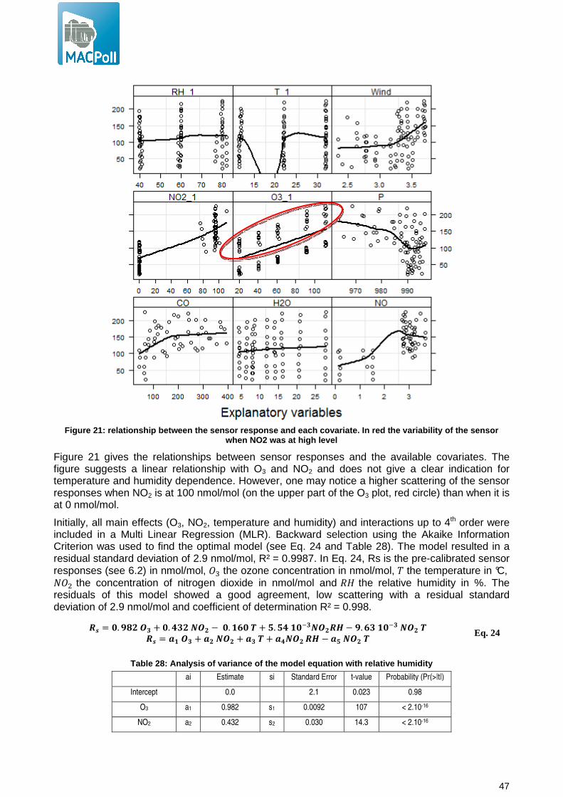
47
Figure 21: relationship between the sensor response and each covariate. In red the variability of the sensor
when NO2 was at high level
Figure 21 gives the relationships between sensor responses and the available covariates. The figure suggests a linear relationship with O3 and NO2 and does not give a clear indication for temperature and humidity dependence. However, one may notice a higher scattering of the sensor responses when NO2 is at 100 nmol/mol (on the upper part of the O3 plot, red circle) than when it is at 0 nmol/mol.
Initially, all main effects (O3, NO2, temperature and humidity) and interactions up to 4th order were included in a Multi Linear Regression (MLR). Backward selection using the Akaike Information Criterion was used to find the optimal model (see Eq. 24 and Table 28). The model resulted in a residual standard deviation of 2.9 nmol/mol, R² = 0.9987. In Eq. 24, Rs is the pre-calibrated sensor responses (see 6.2) in nmol/mol, �� the ozone concentration in nmol/mol, � the temperature in °C, ��� the concentration of nitrogen dioxide in nmol/mol and �� the relative humidity in %. The residuals of this model showed a good agreement, low scattering with a residual standard deviation of 2.9 nmol/mol and coefficient of determination R² = 0.998.
&� = 3.45�6/ + 3.7 �'6� − 3.�839 + :.:7�3�/'6�&; − 4.8 �3�/'6�9 &� = <�6/ + <�'6� + </9 + <1'6�&; − <3'6�9 Eq. 24
Table 28: Analysis of variance of the model equatio n with relative humidity
ai Estimate si Standard Error t-value Probability (Pr(>|t|)
Intercept 0.0 2.1 0.023 0.98
O3 a1 0.982 s1 0.0092 107 < 2.10-16
NO2 a2 0.432 s2 0.030 14.3 < 2.10-16
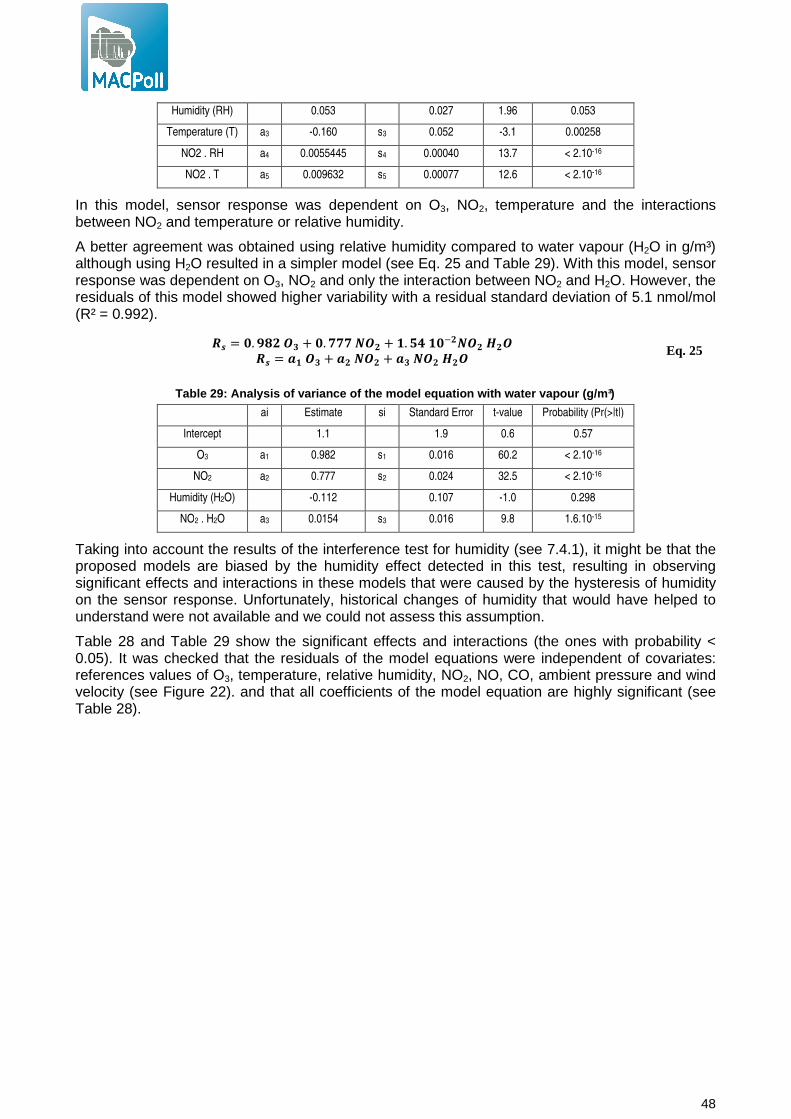
48
Humidity (RH) 0.053 0.027 1.96 0.053
Temperature (T) a3 -0.160 s3 0.052 -3.1 0.00258
NO2 . RH a4 0.0055445 s4 0.00040 13.7 < 2.10-16
NO2 . T a5 0.009632 s5 0.00077 12.6 < 2.10-16
In this model, sensor response was dependent on O3, NO2, temperature and the interactions between NO2 and temperature or relative humidity.
A better agreement was obtained using relative humidity compared to water vapour (H2O in g/m³) although using H2O resulted in a simpler model (see Eq. 25 and Table 29). With this model, sensor response was dependent on O3, NO2 and only the interaction between NO2 and H2O. However, the residuals of this model showed higher variability with a residual standard deviation of 5.1 nmol/mol (R² = 0.992).
&� = 3.45�6/ + 3.==='6� + �.:7�3��'6�;�6 &� = <�6/ + <�'6� + </'6�;�6 Eq. 25
Table 29: Analysis of variance of the model equatio n with water vapour (g/m³)
ai Estimate si Standard Error t-value Probability (Pr(>|t|)
Intercept 1.1 1.9 0.6 0.57
O3 a1 0.982 s1 0.016 60.2 < 2.10-16
NO2 a2 0.777 s2 0.024 32.5 < 2.10-16
Humidity (H2O) -0.112 0.107 -1.0 0.298
NO2 . H2O a3 0.0154 s3 0.016 9.8 1.6.10-15
Taking into account the results of the interference test for humidity (see 7.4.1), it might be that the proposed models are biased by the humidity effect detected in this test, resulting in observing significant effects and interactions in these models that were caused by the hysteresis of humidity on the sensor response. Unfortunately, historical changes of humidity that would have helped to understand were not available and we could not assess this assumption.
Table 28 and Table 29 show the significant effects and interactions (the ones with probability < 0.05). It was checked that the residuals of the model equations were independent of covariates: references values of O3, temperature, relative humidity, NO2, NO, CO, ambient pressure and wind velocity (see Figure 22). and that all coefficients of the model equation are highly significant (see Table 28).
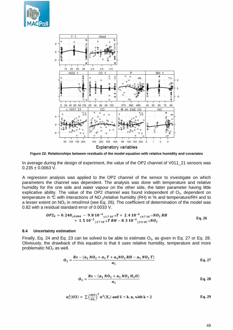
49
Figure 22: Relationships between residuals of the m odel equation with relative humidity and covariates
In average during the design of experiment, the value of the OP2 channel of V011_21 sensors was 0.235 ± 0.0063 V.
A regression analysis was applied to the OP2 channel of the sensor to investigate on which parameters the channel was dependent. The analysis was done with temperature and relative humidity for the one side and water vapour on the other side, the latter parameter having little explicative ability. The value of the OP2 channel was found independent of O3, dependent on temperature in °C with interactions of NO 2/relative humidity (RH) in % and temperature/RH and to a lesser extent on NO2 in nmol/mol (see Eq. 26). The coefficient of determination of the model was 0.82 with a residual standard error of 0.0033 V.
6>�4 = 3.�73±5.551 − 4.5�3�1±�.6�5��9+ �.7�3�7±1.6�5��'6�&;+ �.:�3�3±�.6�5��9&;−5. �3�3±�."�5��'6�
Eq. 26
8.4 Uncertainty estimation
Finally, Eq. 24 and Eq. 23 can be solved to be able to estimate O3, as given in Eq. 27 or Eq. 28. Obviously, the drawback of this equation is that it uses relative humidity, temperature and more problematic NO2 as well.
6/ =&? − �<�'6� + </9 + <1'6�&; − <3'6�9�<� Eq. 27
6/ =&?− �<�'6� + </'6�;�6�<� Eq. 28
@8��6 � = ∑ �9:/
9;�
�� @��A*� and U = k. uc with k = 2 Eq. 29
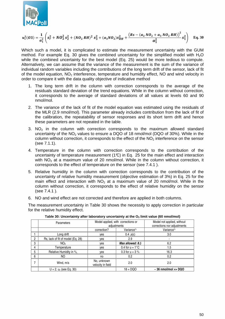
50
@8��6 � = �
<�� B��� +���� ��
�+ �'6�&;����� + �</'6������ +
C&? − �<�'6� + </'6�&;�D����
���E Eq. 30
Which such a model, it is complicated to estimate the measurement uncertainty with the GUM method. For example Eq. 30 gives the combined uncertainty for the simplified model with H2O while the combined uncertainty for the best model (Eq. 25) would be more tedious to compute. Alternatively, we can assume that the variance of the measurement is the sum of the variance of individual random variables including the contributions of the long term drift of the sensor, lack of fit of the model equation, NO2 interference, temperature and humidity effect, NO and wind velocity in order to compare it with the data quality objective of indicative method
1. The long term drift in the column with correction corresponds to the average of the residuals standard deviation of the trend equations. While in the column without correction, it corresponds to the average of standard deviations of all values at levels 60 and 90 nmol/mol.
2. The variance of the lack of fit of the model equation was estimated using the residuals of the MLR (2.9 nmol/mol). This parameter already includes contribution from the lack of fit of the calibration, the repeatability of sensor responses and its short term drift and hence these parameters are not repeated in the table.
3. NO2 in the column with correction corresponds to the maximum allowed standard uncertainty of the NO2 values to ensure a DQO of 18 nmol/mol (DQO of 30%). While in the column without correction, it corresponds to the effect of the NO2 interference on the sensor (see 7.1.1).
4. Temperature in the column with correction corresponds to the contribution of the uncertainty of temperature measurement (1°C) in Eq. 25 for the main effect and interaction with NO2 at a maximum value of 20 nmol/mol. While in the column without correction, it corresponds to the effect of temperature on the sensor (see 7.4.1 ).
5. Relative humidity in the column with correction corresponds to the contribution of the uncertainty of relative humidity measurement (objective estimation of 3%) in Eq. 25 for the main effect and interaction with NO2 at a maximum value of 20 nmol/mol. While in the column without correction, it corresponds to the effect of relative humidity on the sensor (see 7.4.1 ).
6. NO and wind effect are not corrected and therefore are applied in both columns.
The measurement uncertainty in Table 30 shows the necessity to apply correction in particular for the relative humidity effect.
Table 30: Uncertainty after laboratory uncertainty at the O 3 limit value (60 nmol/mol)
Parameters Model applied, with corrections or adjustments
Model not applied, without corrections nor adjustments
correction? Variance½ Variance½
1 Long drift yes 0.4 ,s(ε) 3.0
2 Rs, lack of fit of model (Eq. 28) yes 2.9 -
3 NO2 yes Max allowed: 8.3 6.2
4 Temperature yes 0.4 for u = 1°C 1.5
5 Relative Humidity in %, yes 0.3 for u = 3 % 16.3
6 NO no 0.2 0.2
7 Wind, m/s No, unknown
velocity in field 2.0 2.0
U = 2. uc (see Eq. 30) 18 = DQO ~ 36 nmol/mol >> DQO

51
9 Field experiments
9.1 Monitoring stations
The JRC station for atmospheric research (45°48.881 ’N, 8°38.165’E, 209 m asl) is located by the Northern fence of the JRC-Ispra site (Fig. 1), situated in a semi-rural area at the NW edge of the Po valley. The station is several tens of km away from large emission sources like intense road traffic or big factories. The main cities around are Varese, 20 km east, Novara, 40 km south, Gallarate - Busto Arsizio, about 20 km south-east and the Milan conurbation, 60 km to the south-east. Busy roads and highways link these urban centers. Four industrial large source points (CO emissions > 1000 tons / yr) are located between 20 and 50 km E to SE of Ispra. The closest (20 km SSE) emits also > 2000 tons of NOx per year. The aim of the JRC-Ispra station is to monitor the concentration of pollutants in the gas phase, the particulate phase and precipitations, as well as aerosol optical parameters, which can be used for assessing the impact of European policies on air pollution and climate change. Measurements are performed in the framework of international monitoring programs like the Co-operative program for monitoring and evaluation of the long range transmission of air pollutants in Europe (EMEP) of the UN-ECE Convention on Long-Range Transboundary Air Pollution (CLRTAP) and the Global Atmosphere Watch (GAW) Program of the World Meteorological Organization (WMO).
From April 2012 until October 2012, a mobile laboratory was installed near the EMEP station sited at Ispra, equipped with routine analysers normally installed in the containers. Gases were sampled using a sampling line (see Figure 23) placed at the top of the roof of the van at about 3.5 m above the ground and on the roof of the mobile laboratory. The sampling line consists in a stainless steel gas inlet with grid protection for rain, insects and dust. The stainless steel inlet tube of 4 cm internal diameter with internal PTFE tube that ends with a Teflon manifold of 8 PTFE ports to connect the gas analysers. The sampling line is flushed with ambient air with about 2 second residentime of samples in the sampling line. Each instrument samples from the glass tube with its own pump through a ¼” PTFE/PFE tube and a 1 µm pore size 47 mm diameter Teflon filter to eliminate particles from the sampled air.
The mobile laboratory was equipped with meteorological sensors and gas analysers which were calibrated in laboratory before the in-situ measurements and then checked every month. Field checks were carried out using zero air in gas cylinders and a span value (internally certified gas cylinders at low concentration for NO/NOx and SO2, highly concentrated cylinders for CO and ozone generator do O3). The highest observed drift of calibration was 3 %, consistent with the uncertainty of the working standards used on field. Therefore, no corrections of measurements were undergone apart from the discarding values during maintenance and calibration checks.
• Meteorological parameters (ambient temperature, ambient relative humidity, ambient pressure, 10m mast for wind speed and wind direction) a mobile. The mobile laboratory was equipped with:
• Gaseous pollutants: for O3 an UV Photometric Analyzer Thermo Environment 49C; for NO2/NO/NOx a Chemiluminescence Nitrogen Oxides Analyzer Thermo 42C; for CO a non-Dispersive Infrared Gas-Filter Correlation Spectroscopy Thermo 48C-TL, for SO2 and UV Fluorescent Analyser Thermo 43C TL
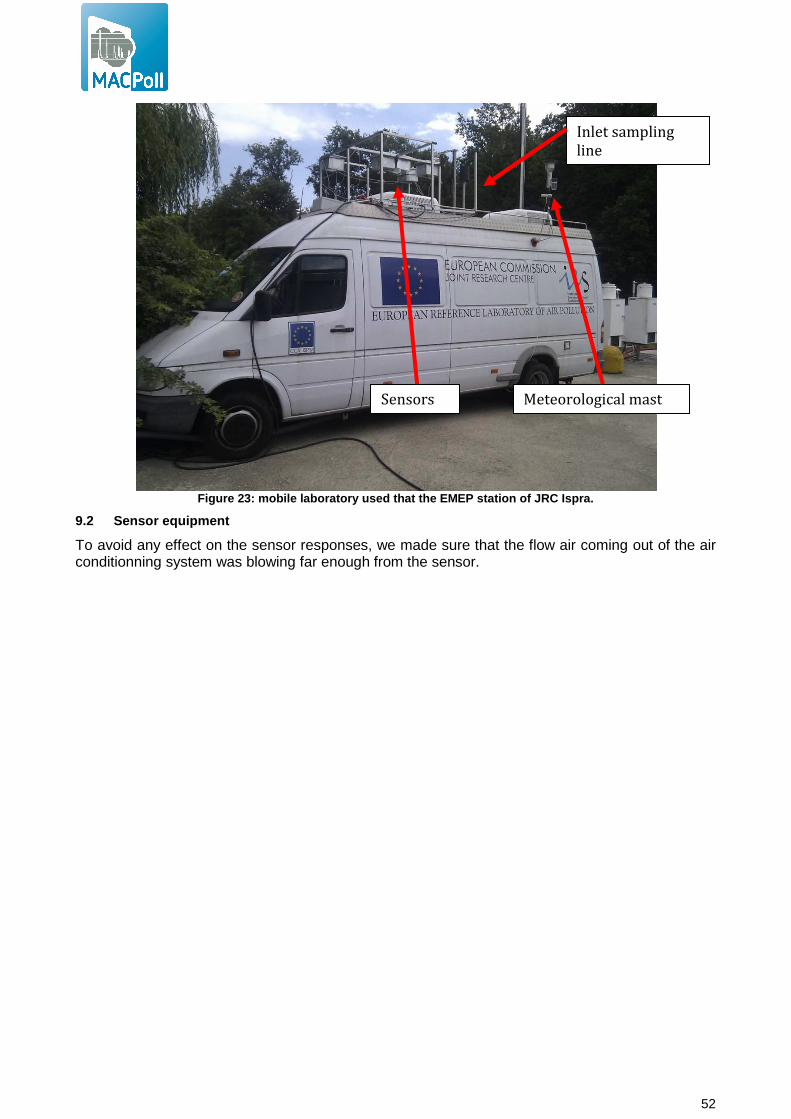
52
Figure 23: mobile laboratory used that the EMEP statio n of JRC Ispra.
9.2 Sensor equipment
To avoid any effect on the sensor responses, we made sure that the flow air coming out of the air conditionning system was blowing far enough from the sensor.
Sensors Meteorological mast
Inlet sampling
line
Figure
9.3 Check of the sensor in laboratory
Hopefully, the sensor should have been the exposure chamber was busy with the laboratory tests for all sensors when receiving the field sensors and the laboratory check had to be postponed to the end of the field experiment. Subsequently, the field sensors were submitted to a lab tests at the end of the field experiments as described in 7.3. NO2, temperature and humidity were kept under controlrelative conditions of the test were set at 22°c an d 60 % of relative humidity, the defined mean values.
The results of the experiment are given in sufficient for this sensor. Consequently, it is expected that the sensor will give nearly linear responses for the field experiment.
The pre-calibration functions were established by plotting sensor responses versus reference values measured by the TECO 49C analyser at stable conditions 22 °C and 60 % (see relative humidity. Each steps lasted for 150 minutes once the condition of Otemperature and humidity were reached. The averages of the last 60 minutes are plotted. In all the following tests this pre-calibration is ap
Figure 24 Sensors location at the monitoring station
Check of the sensor in laboratory
Hopefully, the sensor should have been tested in laboratory before installation in field. However, the exposure chamber was busy with the laboratory tests for all sensors when receiving the field sensors and the laboratory check had to be postponed to the end of the field experiment.
ly, the field sensors were submitted to a lab tests at the end of the field experiments as , temperature and humidity were kept under control.
relative conditions of the test were set at 22°c an d 60 % of relative humidity, the defined mean
The results of the experiment are given in Figure 25 which shows that a simple linear equation sufficient for this sensor. Consequently, it is expected that the sensor will give nearly linear responses for the field experiment.
calibration functions were established by plotting sensor responses versus reference values measured by the TECO 49C analyser at stable conditions 22 °C and 60 % (see
Each steps lasted for 150 minutes once the condition of Otemperature and humidity were reached. The averages of the last 60 minutes are plotted. In all the
calibration is applied before data analysis. One may notice a decrease in
53
tested in laboratory before installation in field. However, the exposure chamber was busy with the laboratory tests for all sensors when receiving the field sensors and the laboratory check had to be postponed to the end of the field experiment.
ly, the field sensors were submitted to a lab tests at the end of the field experiments as The temperature and
relative conditions of the test were set at 22°c an d 60 % of relative humidity, the defined mean
simple linear equation was sufficient for this sensor. Consequently, it is expected that the sensor will give nearly linear
calibration functions were established by plotting sensor responses versus reference values measured by the TECO 49C analyser at stable conditions 22 °C and 60 % (see Figure 7) of
Each steps lasted for 150 minutes once the condition of O3 concentrations, temperature and humidity were reached. The averages of the last 60 minutes are plotted. In all the
plied before data analysis. One may notice a decrease in
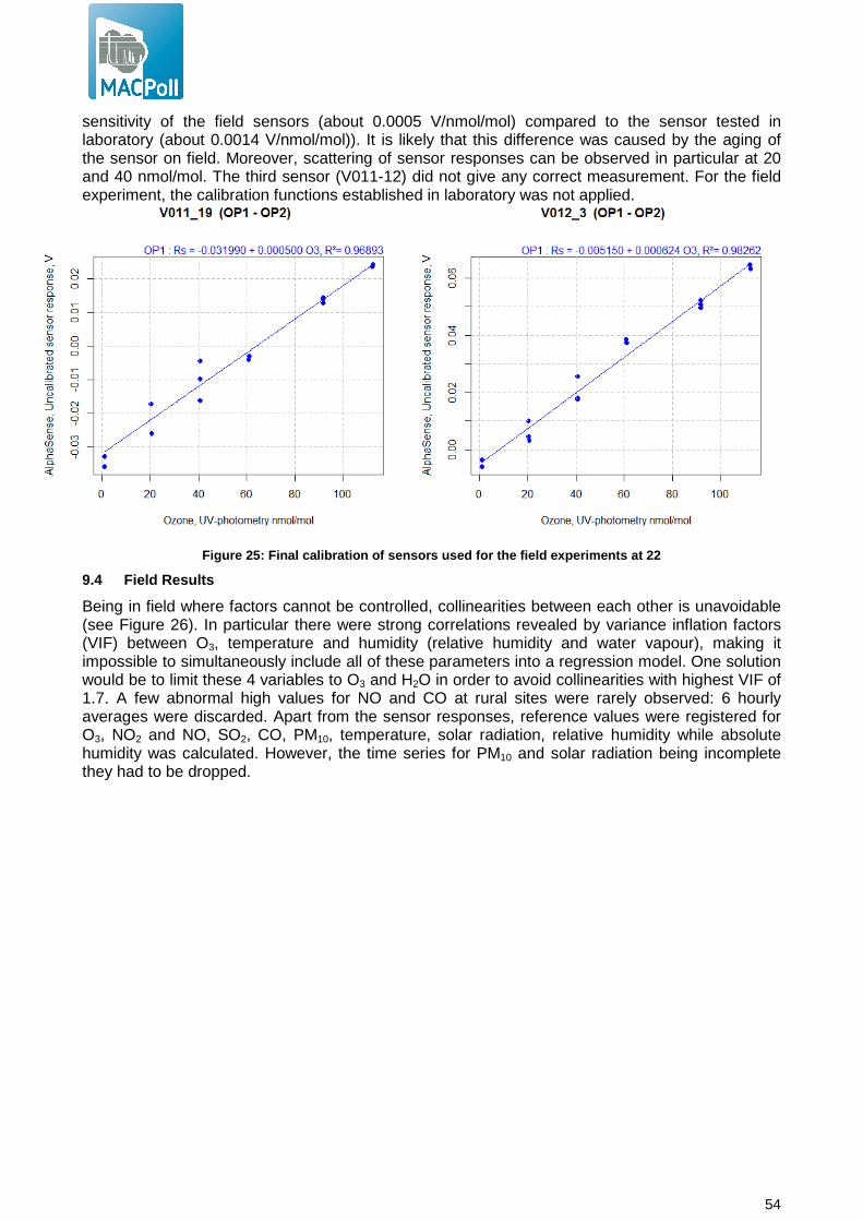
54
sensitivity of the field sensors (about 0.0005 V/nmol/mol) compared to the sensor tested in laboratory (about 0.0014 V/nmol/mol)). It is likely that this difference was caused by the aging of the sensor on field. Moreover, scattering of sensor responses can be observed in particular at 20 and 40 nmol/mol. The third sensor (V011-12) did not give any correct measurement. For the field experiment, the calibration functions established in laboratory was not applied.
Figure 25: Final calibration of sensors used for th e field experiments at 22
9.4 Field Results
Being in field where factors cannot be controlled, collinearities between each other is unavoidable (see Figure 26). In particular there were strong correlations revealed by variance inflation factors (VIF) between O3, temperature and humidity (relative humidity and water vapour), making it impossible to simultaneously include all of these parameters into a regression model. One solution would be to limit these 4 variables to O3 and H2O in order to avoid collinearities with highest VIF of 1.7. A few abnormal high values for NO and CO at rural sites were rarely observed: 6 hourly averages were discarded. Apart from the sensor responses, reference values were registered for O3, NO2 and NO, SO2, CO, PM10, temperature, solar radiation, relative humidity while absolute humidity was calculated. However, the time series for PM10 and solar radiation being incomplete they had to be dropped.
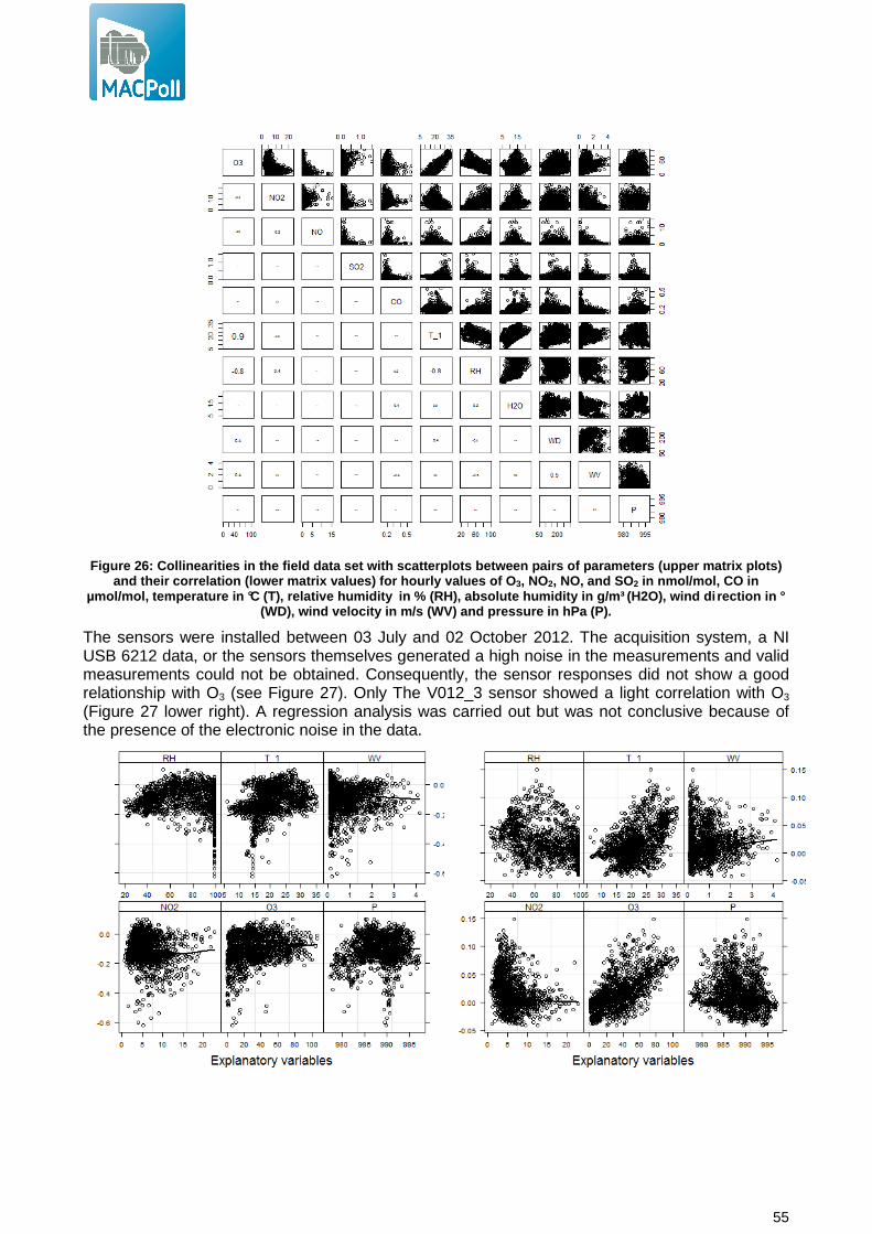
55
Figure 26: Collinearities in the field data set wit h scatterplots between pairs of parameters (upper m atrix plots)
and their correlation (lower matrix values) for hou rly values of O 3, NO2, NO, and SO2 in nmol/mol, CO in µmol/mol, temperature in °C (T), relative humidity in % (RH), absolute humidity in g/m³ (H2O), wind di rection in °
(WD), wind velocity in m/s (WV) and pressure in hPa ( P).
The sensors were installed between 03 July and 02 October 2012. The acquisition system, a NI USB 6212 data, or the sensors themselves generated a high noise in the measurements and valid measurements could not be obtained. Consequently, the sensor responses did not show a good relationship with O3 (see Figure 27). Only The V012_3 sensor showed a light correlation with O3
(Figure 27 lower right). A regression analysis was carried out but was not conclusive because of the presence of the electronic noise in the data.
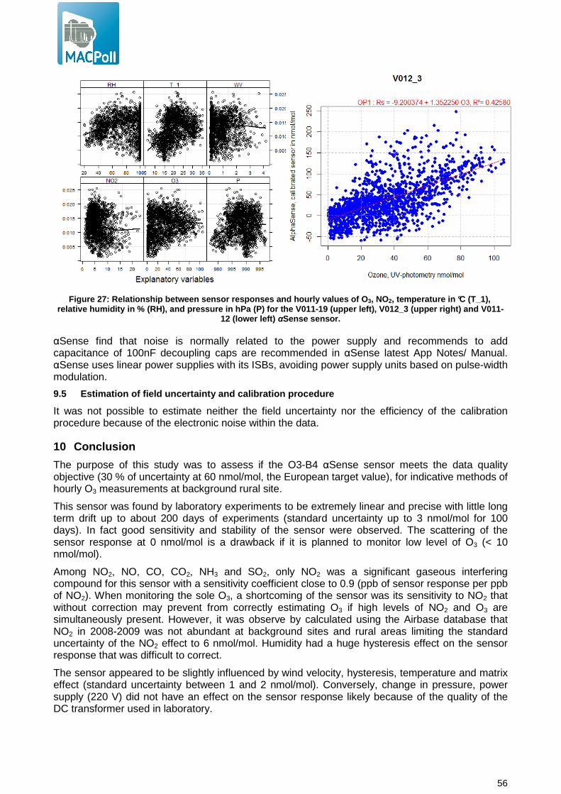
56
Figure 27: Relationship between sensor responses an d hourly values of O 3, NO2, temperature in °C (T_1), relative humidity in % (RH), and pressure in hPa (P) for the V011-19 (upper left), V012_3 (upper right) an d V011-
12 (lower left) αSense sensor.
αSense find that noise is normally related to the power supply and recommends to add capacitance of 100nF decoupling caps are recommended in αSense latest App Notes/ Manual. αSense uses linear power supplies with its ISBs, avoiding power supply units based on pulse-width modulation.
9.5 Estimation of field uncertainty and calibration procedure
It was not possible to estimate neither the field uncertainty nor the efficiency of the calibration procedure because of the electronic noise within the data.
10 Conclusion
The purpose of this study was to assess if the O3-B4 αSense sensor meets the data quality objective (30 % of uncertainty at 60 nmol/mol, the European target value), for indicative methods of hourly O3 measurements at background rural site.
This sensor was found by laboratory experiments to be extremely linear and precise with little long term drift up to about 200 days of experiments (standard uncertainty up to 3 nmol/mol for 100 days). In fact good sensitivity and stability of the sensor were observed. The scattering of the sensor response at 0 nmol/mol is a drawback if it is planned to monitor low level of O3 (< 10 nmol/mol).
Among NO2, NO, CO, CO2, NH3 and SO2, only NO2 was a significant gaseous interfering compound for this sensor with a sensitivity coefficient close to 0.9 (ppb of sensor response per ppb of NO2). When monitoring the sole O3, a shortcoming of the sensor was its sensitivity to NO2 that without correction may prevent from correctly estimating O3 if high levels of NO2 and O3 are simultaneously present. However, it was observe by calculated using the Airbase database that NO2 in 2008-2009 was not abundant at background sites and rural areas limiting the standard uncertainty of the NO2 effect to 6 nmol/mol. Humidity had a huge hysteresis effect on the sensor response that was difficult to correct.
The sensor appeared to be slightly influenced by wind velocity, hysteresis, temperature and matrix effect (standard uncertainty between 1 and 2 nmol/mol). Conversely, change in pressure, power supply (220 V) did not have an effect on the sensor response likely because of the quality of the DC transformer used in laboratory.

57
With the laboratory experiments, simple models were established to compute O3 using the sensors responses, NO2 and water vapour or both temperature and relative humidity.
The sensor measurement uncertainty, calculated using the results of all laboratory experiments could meet the Data Quality Objective (30 % of relative expanded uncertainty) only if these models were applied. Without applying these models, the contribution of humidity and NO2 was found too high (> 36 nmol/mol at 60 nmol/mol of O3, the European target value).
The sensors, used in field, were calibrated in laboratory at the end of the field exposure of about 4 months. Unfortunately, the field experiments were not successful and valid measurements could not be obtained. Therefore, the models established with the laboratory experiments could not be verified in field.
Further to this study, the application of the sensor as indicative method for O3 fixed measurement at background site/rural areas is not fully validated. In fact, field confirmation of the laboratory results which gave satisfaction provided that a correction was used is missing.
The manufacturer, αSense, agreed on the lack of speciation between O3 and NO2 of the sensor and its humidity dependence. αSense has been working on speciation of O3 and NO2 for a long time and is expecting to find a solution to this problem soon13. Humidity dependence is going to be the next shortcoming that the company is going to tackle using correction algorithms in collaboration with the group of Prof. Roderick Jones in Cambridge.
Even though the O3 B4 sensor is not fully selective, it produces repeatable values that might be improved in the future with sophisticated algorithms to ensure sensitivity, selectivity and stability requirements for sensors.
13 See “Measuring ppb gas concentrations using air quality networks”, John Saffell (Alphasense, Ltd., UK), Air Sensors 2014: A New Frontier Monitoring Technology for Today's World, June 9 & 10, 2014, EPA's Research Triangle Park Campus, 109 T.W. Alexander Drive, Research Triangle Park, North Carolina 27711

58
11 Appendix A: Data sheet of αSense 4-electrode O3-B4 and Individual Sensor Board (ISB) Issue 4, 085-2217 User Manual Issue 2
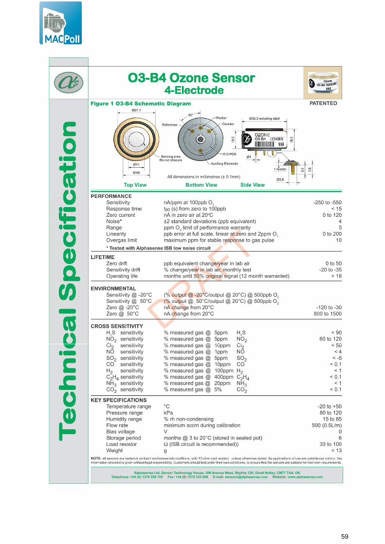
59
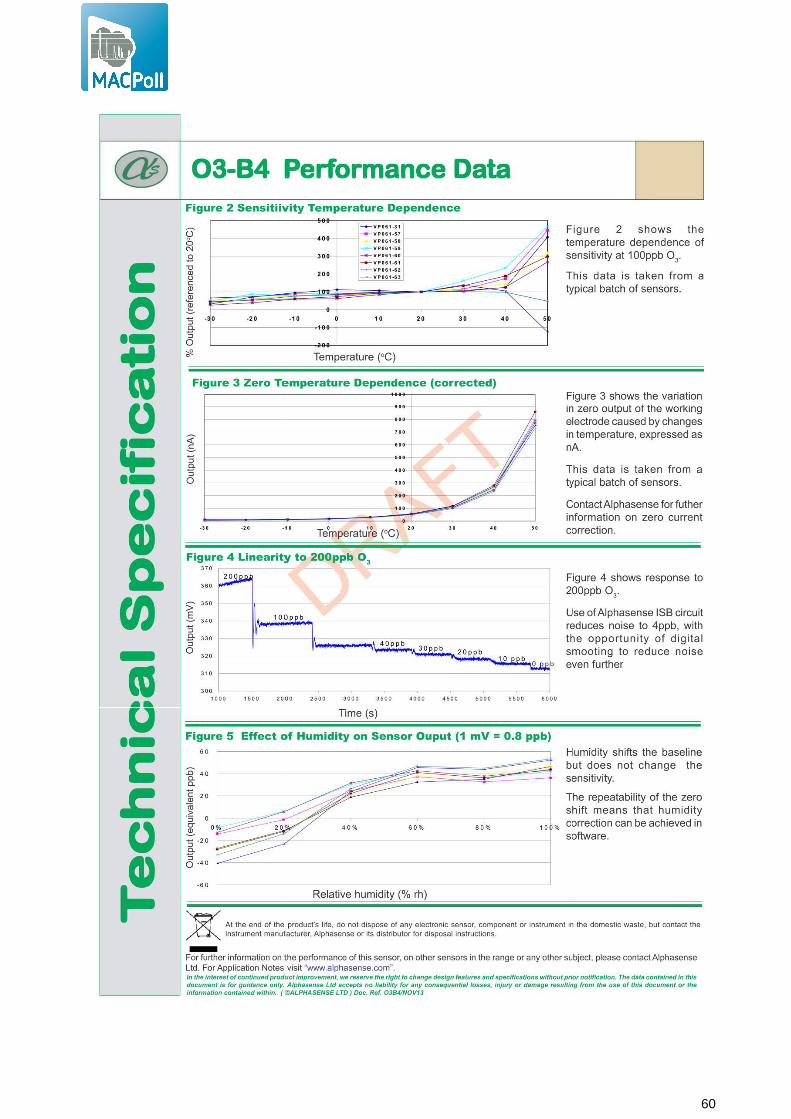
60
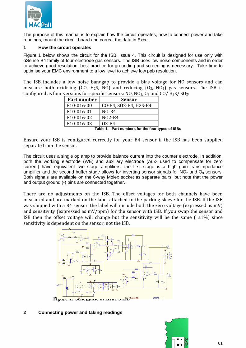
61
The purpose of this manual is to explain how the circuit operates, how to connect power and take readings, mount the circuit board and correct the data in Excel.
1 How the circuit operates
Figure 1 below shows the circuit for the ISB, issue 4. This circuit is designed for use only with αSense B4 family of four-electrode gas sensors. The ISB uses low noise components and in order to achieve good resolution, best practice for grounding and screening is necessary. Take time to optimise your EMC environment to a low level to achieve low ppb resolution. The ISB includes a low noise bandgap to provide a bias voltage for NO sensors and can
measure both oxidising (CO, H2S, NO) and reducing (O3, NO2) gas sensors. The ISB is
configured as four versions for specific sensors: NO, NO2, O3 and CO/ H2S/ SO2:
Part number Sensor
810-016-00 CO-B4, SO2-B4, H2S-B4
810-016-01 NO-B4
810-016-02 NO2-B4
810-016-03 O3-B4 Table 1. Part numbers for the four types of ISBs
Ensure your ISB is configured correctly for your B4 sensor if the ISB has been supplied
separate from the sensor. The circuit uses a single op amp to provide balance current into the counter electrode. In addition, both the working electrode (WE) and auxiliary electrode (Aux- used to compensate for zero current) have equivalent two stage amplifiers: the first stage is a high gain transimpedance amplifier and the second buffer stage allows for inverting sensor signals for NO2 and O3 sensors. Both signals are available on the 6-way Molex socket as separate pairs, but note that the power and output ground (-) pins are connected together.
There are no adjustments on the ISB. The offset voltages for both channels have been
measured and are marked on the label attached to the packing sleeve for the ISB. If the ISB
was shipped with a B4 sensor, the label will include both the zero voltage (expressed as mV)
and sensitivity (expressed as mV/ppm) for the sensor with ISB. If you swap the sensor and
ISB then the offset voltage will change but the sensitivity will be the same ( ±1%) since
sensitivity is dependent on the sensor, not the ISB.
Figure 1. Schematic of Issue 3 ISB
2 Connecting power and taking readings

62
The socket for power and signals is shown in figure 2 below.
The Molex socket is polarised.
Figure 2. ISB socket for power and signals
DC power is required: 6.0 ±0.2 VDC. Ensure your power supply is low noise and decoupled, or its noise component will be added to the measured signal.
OP1 is the signal from the Working Electrode and OP2 is the signal from the Auxiliary Electrode.
The –ve pins are connected so you can use either 6-way or 4-way cable to connect to the ISB. OP1 and OP2 are buffered DC signals so a normal A/D converter will be fine, so long as it does not inject noise back into the ISB. If you are concerned about noise injection, then decouple using 10nF plus 100nF capacitors close to the Molex connector.
Table 2 below lists expected outputs from ISB with a typical B4 sensor.
Gas Zero offset mV (WE / Aux)
sensitivity mV/ppm
Min/ max sensitivity mV/ppm
Full scale ppm
Gain mV/nA
CO 270/ 340 320 230/ 550 15 1.76 H2S 350/ 350 1650 1600/ 1700 3 1.76 SO2 355/ 345 450 370/ 520 10 1.76 NO 545/ 510 800 550/ 930 5 2.53 NO2 225/ 245 430 340/ 520 10 1.24 O3 260/ 300 1150 1000/1200 5 1.01 Table 2. Offset, sensitivity and full scale for ty pical B4 sensors with ISB
Noise 1 These gas sensors are very sensitive to gas and are also very susceptible to EMC
pickup. Ideally the sensors would be housed in a Faraday cage, but this is not normally
practicable, so shield and ground as best you can. Nearby digital circuits can also
disrupt the signal quality.
2 Typical noise at αSense, when calibrating on a bench without additional shielding, but
with good power supply is 3 mV (p-p). Digital averaging can reduce this to less than
one mV, equivalent to typically 2 ppb. Further reduction of noise can be achieved by
shielding.
3 It is important to decouple your power supply and A/D converter from the ISB. Since
the 0V line is shared by the power supply and output, any noise injected by your power
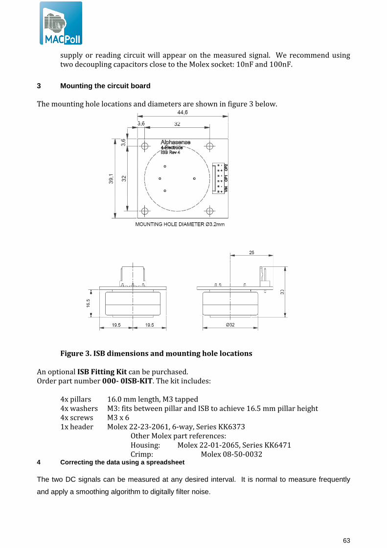
63
supply or reading circuit will appear on the measured signal. We recommend using
two decoupling capacitors close to the Molex socket: 10nF and 100nF.
3 Mounting the circuit board
The mounting hole locations and diameters are shown in figure 3 below.
Figure 3. ISB dimensions and mounting hole locations
An optional ISB Fitting Kit can be purchased.
Order part number 000- 0ISB-KIT. The kit includes:
4x pillars 16.0 mm length, M3 tapped
4x washers M3: fits between pillar and ISB to achieve 16.5 mm pillar height
4x screws M3 x 6
1x header Molex 22-23-2061, 6-way, Series KK6373
Other Molex part references:
Housing: Molex 22-01-2065, Series KK6471
Crimp: Molex 08-50-0032 4 Correcting the data using a spreadsheet The two DC signals can be measured at any desired interval. It is normal to measure frequently
and apply a smoothing algorithm to digitally filter noise.

64
The method for determining the concentration depends on whether you have purchased sensor
with ISB or sensor and ISB separately. αSense recommends purchasing the ISB and sensor
together- this allows us to measure accurately the zero gas voltage before shipping.
4.1 Measuring when the ISB and sensor were shipped together Create a spreadsheet similar to the layout below:
Vo (OP1) Vo(OP2) mV/ppm
Time WE (OP1) WE- Vo Aux
(OP2)
Aux-Vo ppm We-Aux ppm
Each column is specified as:
Column Label Cell data Comments A Time From your data acquisition
system Sampling faster than 1 second is rarely useful unless it reduces noise.
B WE (OP1) mV from ISB channel 1 0.1 mV resolution is ideal C WE-Vo Column B- Vo (constant
specified on ISB bag label) Subtract the WE offset voltage- typical values are the second column in table 2.
D Aux (OP2) mV from ISB channel 2 0.1 mV resolution is ideal. E Aux-Vo Column D- Vo (constant
specified on ISB bag label) Calculates the Aux offset voltage shift- typical Vo are the second column in table 2.This difference is a few mV.
F ppm Column C * sensitivity (specified on ISB bag label)
ppm calculated from the sensitivity constant (mV/ppm), corrected for offset voltage but not the auxiliary electrode.
G WE-Aux Column C – Column E Correction for any drift in the auxiliary and WE (as mV)
H ppm Column G * sensitivity (specified on ISB bag label)
ppm, corrected for offset drift
Table 3. Typical data spreadsheet layout and cell a ssignment
4.2 Measuring when the ISB and sensor were shipped separately If the ISB and sensor were shipped separately then set up the same spreadsheet as above, but
the zero voltage will be for the ISB only and does not include the sensor. You must measure
the zero voltage with the sensor connected to the ISB:
Plug sensor into ISB and apply 6 VDC to power the sensor/ISB pair.
1 Allow to stabilise in clean air for at least 6 hours.
2 Apply zero air (synthetic air or scrubbed/ cleaned zero air) for 20 minutes.
3 Record Vo for both WE (OP1) and Aux (OP2). Enter these values in cells C1 and E1.
Additionally, the sensor is calibrated as nA/ ppm but this must be converted to mV/ppm. The
last column in Table 2 lists the scaling constant which must be applied for your sensor type.
The ISBs have a gain that is repeatable ±1.2% (95% confidence interval) so this conversion
constant is the same for all ISBs for a specific sensor/ gas.
4.3 Recalibration

65
The ISB with sensor calibration has been measured before leaving the factory, but
environmental conditions and sensor drift mean that periodic checking of the calibration may
be required.
Also, at low ppb concentrations both temperature and humidity will affect the offset voltage of
both the WE and Auxiliary electrodes. Previously it was thought that simple subtraction of the
Auxiliary would correct for ambient changes but this is not true. Contact αSense for
assistance in use of the correct method for compensation in your application.
4.3.1 Zero correction Follow the procedure in 4.2 above and modify the Vo mV in your spreadsheet after zero
calibration. Be careful that the zero air you use is very clean: ambient or lab air is not
sufficiently clean to be used as a zero calibration air source.
4.3.2 Gain/ sensitivity correction Unless you have access to an accurate 1 ppm or less gas supply, it is advised to return
(sensor + ISB) to αSense for gain recalibration.
End of User Manual
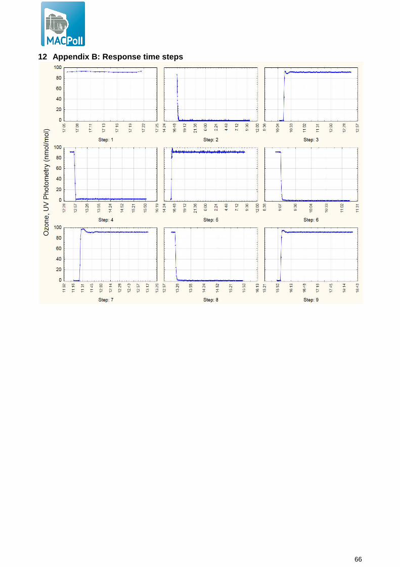
66
12 Appendix B: Response time steps
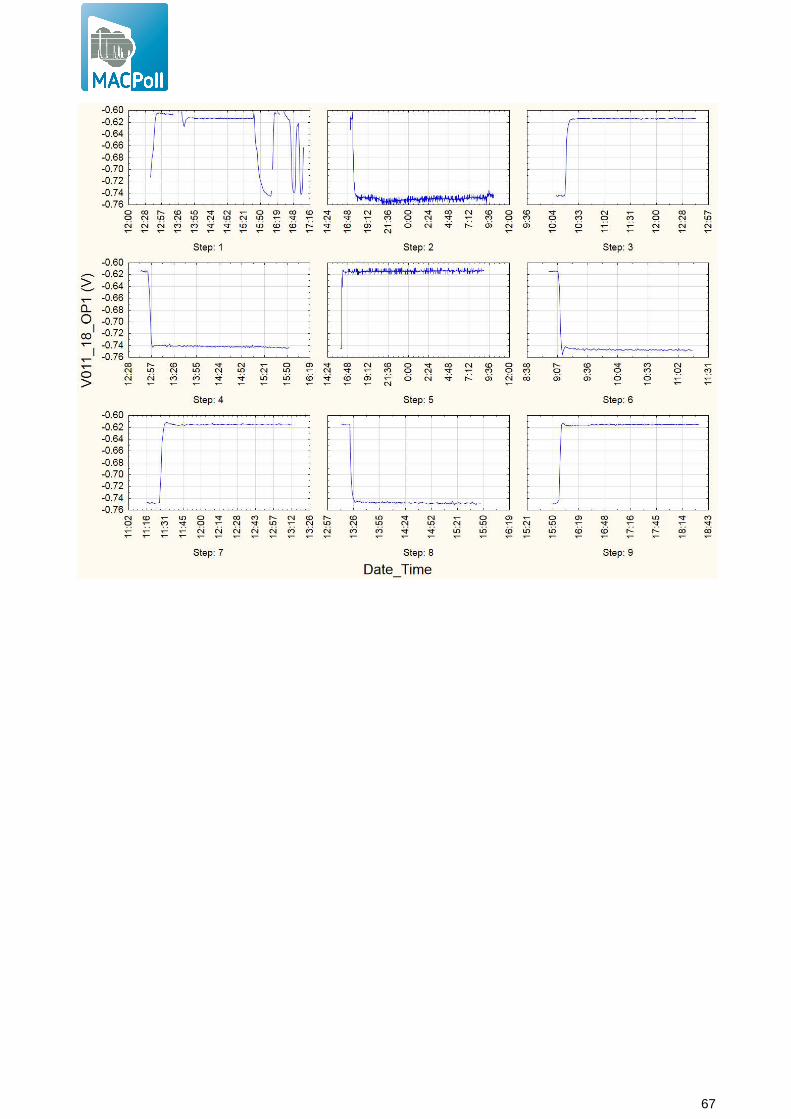
67
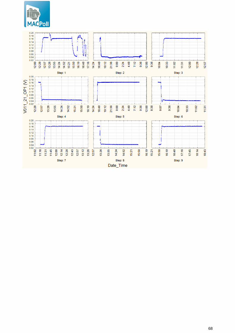
68
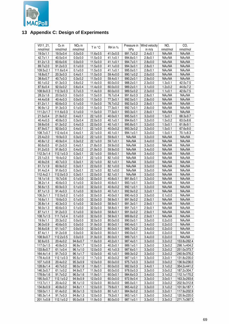
69
13 Appendix C: Design of Experiments
V011_21, nmol/mol
O3 in nmol/mol
NO2 in nmol/mol
T in °C RH in % Pressure in
hPa Wind velocity
in m/s NO,
nmol/mol CO,
nmol/mol
19.0±1.1 19.5±0.4 0.0±0.0 11.6±0.5 41.0±0.5 991.7±0.2 2.4±0.1 NA±NA NA±NA
42.7±1.1 40.5±0.4 0.0±0.0 11.5±0.0 41.1±0.1 994.8±0.1 2.8±0.1 NA±NA NA±NA
61.2±1.3 60.6±0.6 0.0±0.0 11.5±0.0 41.1±0.1 994.7±0.1 2.8±0.0 NA±NA NA±NA
89.7±2.0 91.2±0.3 0.1±0.0 11.5±0.0 41.1±0.0 994.3±0.1 2.8±0.1 NA±NA NA±NA
109.5±2.1 111.6±0.4 0.1±0.0 11.5±0.0 41.1±0.1 995.0±0.1 2.8±0.1 NA±NA NA±NA
18.8±0.7 20.3±0.3 0.4±0.1 11.5±0.0 59.4±0.0 990.1±0.2 2.6±0.0 NA±NA NA±NA
38.6±0.7 40.7±0.3 0.3±0.2 11.5±0.0 59.4±0.1 990.2±0.1 2.9±0.0 NA±NA NA±NA
60.1±0.2 61.3±0.3 0.6±0.2 11.4±0.0 60.0±0.0 988.2±0.1 2.3±0.0 1.3±0.1 42.5±7.5
87.6±0.4 92.0±0.2 0.6±0.4 11.4±0.0 60.0±0.0 989.2±0.1 3.1±0.0 1.2±0.2 44.6±7.2
108.9±0.3 112.3±0.3 0.7±0.3 11.4±0.0 60.0±0.0 989.5±0.2 2.3±0.0 1.1±0.1 42.6±7.5
28.2±1.6 20.0±0.3 0.0±0.0 11.5±0.0 76.7±0.4 991.6±0.3 2.8±0.1 NA±NA NA±NA
44.4±0.8 40.4±0.3 0.0±0.0 11.5±0.0 77.3±0.1 992.5±0.1 2.8±0.0 NA±NA NA±NA
61.2±1.1 60.6±0.3 0.1±0.0 11.5±0.0 76.7±0.2 992.5±0.3 2.8±0.1 NA±NA NA±NA
90.9±1.2 91.3±0.3 0.1±0.0 11.5±0.0 77.3±0.1 992.7±0.1 2.8±0.0 NA±NA NA±NA
111.2±1.7 111.6±0.3 0.1±0.0 11.5±0.0 77.3±0.1 993.3±0.1 2.8±0.1 NA±NA NA±NA
21.5±0.4 21.9±0.2 0.4±0.1 22.1±0.0 40.0±0.1 995.5±0.1 3.2±0.0 1.5±0.1 68.3±9.7
40.4±0.3 40.8±0.3 0.3±0.4 22.0±0.0 40.1±0.1 994.6±0.1 3.2±0.0 1.5±0.2 63.0±8.6
59.8±0.6 61.3±0.2 0.4±0.3 22.0±0.0 40.1±0.1 995.8±0.1 3.2±0.0 1.5±0.1 61.8±9.1
87.9±0.7 92.0±0.3 0.4±0.1 22.1±0.0 40.0±0.2 993.3±0.2 3.2±0.0 1.5±0.1 67.6±9.0
108.7±0.7 112.4±0.4 0.4±0.1 22.1±0.0 40.1±0.1 994.1±0.1 3.2±0.0 1.5±0.1 70.1±8.3
23.4±2.0 19.9±0.3 0.3±0.2 22.1±0.0 59.6±0.1 NA±NA 3.2±0.0 NA±NA NA±NA
40.8±1.2 40.9±0.4 0.3±0.2 22.1±0.0 59.7±0.1 NA±NA 3.4±0.0 NA±NA NA±NA
60.6±0.5 61.2±0.3 0.4±0.1 21.8±0.0 59.9±0.0 NA±NA 3.3±0.0 NA±NA NA±NA
91.2±0.5 91.8±0.3 0.4±0.2 21.9±0.0 59.9±0.0 NA±NA 3.4±0.0 NA±NA NA±NA
112.3±1.4 112.1±0.3 0.3±0.1 22.1±0.0 59.6±0.1 NA±NA 3.4±0.0 NA±NA NA±NA
23.1±2.5 19.4±0.2 0.3±0.1 22.1±0.0 82.1±0.0 NA±NA 3.5±0.0 NA±NA NA±NA
40.9±2.6 40.7±0.3 0.3±0.1 22.1±0.0 82.1±0.1 NA±NA 3.5±0.0 NA±NA NA±NA
61.7±1.9 60.9±0.2 0.3±0.1 22.0±0.0 82.1±0.0 NA±NA 3.5±0.0 NA±NA NA±NA
91.4±2.4 91.6±0.3 0.3±0.1 22.1±0.0 82.1±0.0 NA±NA 3.5±0.0 NA±NA NA±NA
112.4±2.1 112.0±0.3 0.3±0.1 22.0±0.0 82.1±0.1 NA±NA 3.5±0.0 NA±NA NA±NA
18.1±1.6 19.7±0.6 0.1±0.0 32.0±0.0 40.6±0.1 991.8±0.1 3.2±0.0 NA±NA NA±NA
38.2±1.4 40.6±0.3 0.1±0.0 32.0±0.0 40.6±0.1 993.1±0.1 3.3±0.0 NA±NA NA±NA
56.6±1.5 60.9±0.3 0.1±0.0 32.0±0.0 40.6±0.2 992.1±0.1 3.2±0.0 NA±NA NA±NA
87.1±1.3 91.4±0.3 0.1±0.0 32.0±0.0 40.7±0.1 992.9±0.2 3.2±0.1 NA±NA NA±NA
106.2±1.1 112.0±0.2 0.1±0.0 32.0±0.0 40.0±0.1 990.4±0.3 3.5±0.0 0.1±0.0 NA±NA
16.6±1.1 19.6±0.3 0.1±0.0 32.0±0.0 58.9±0.1 991.9±0.2 2.9±0.1 NA±NA NA±NA
35.8±1.4 40.3±0.3 0.1±0.0 32.0±0.0 58.9±0.1 991.3±0.1 2.9±0.1 NA±NA NA±NA
56.0±1.3 60.6±0.3 0.1±0.0 32.0±0.0 58.8±0.1 991.7±0.1 2.9±0.1 NA±NA NA±NA
87.1±1.1 91.2±0.3 0.1±0.0 32.0±0.0 58.8±0.1 991.0±0.2 2.9±0.1 NA±NA NA±NA
108.7±1.5 111.7±0.4 0.1±0.0 32.0±0.0 58.9±0.1 989.8±0.2 2.9±0.1 NA±NA NA±NA
19.9±1.1 20.3±0.2 0.0±0.0 32.0±0.0 80.0±0.0 990.0±0.1 3.5±0.0 0.2±0.0 NA±NA
36.0±0.9 40.6±0.5 0.0±0.0 31.9±0.0 80.0±0.1 990.4±0.1 3.4±0.0 0.2±0.0 NA±NA
56.6±0.8 61.1±0.7 0.0±0.0 32.0±0.0 80.0±0.1 989.7±0.2 3.4±0.0 0.2±0.0 NA±NA
87.4±1.1 91.2±0.8 0.0±0.0 32.0±0.0 80.0±0.1 990.0±0.1 3.4±0.0 0.2±0.0 NA±NA
108.9±0.7 112.2±0.5 0.0±0.0 31.9±0.0 80.0±0.1 989.7±0.1 3.4±0.0 0.2±0.0 NA±NA
92.6±0.5 20.4±0.2 94.6±0.7 11.6±0.0 40.2±0.1 987.4±0.1 3.3±0.0 3.2±0.2 153.8±262.4
117.0±1.5 40.8±0.3 96.9±1.7 12.0±0.0 40.2±0.1 989.1±0.1 3.3±0.0 3.3±0.2 298.1±404.2
133.8±0.7 61.1±0.4 96.1±1.0 12.0±0.0 40.1±0.3 987.6±0.1 3.3±0.0 3.2±0.2 251.0±373.7
164.4±1.4 91.7±0.3 96.1±1.7 12.0±0.0 40.1±0.1 989.3±0.2 3.3±0.0 3.2±0.2 240.9±376.2
178.4±0.8 112.1±0.3 95.5±1.0 11.7±0.0 40.0±0.2 987.1±0.1 3.3±0.0 3.2±0.1 131.8±235.0
107.1±0.8 20.4±0.2 95.3±0.9 12.0±0.0 60.0±0.0 975.7±0.3 3.3±0.0 3.0±0.2 136.9±236.0
128.8±1.4 40.7±0.2 98.0±1.8 11.8±0.1 60.0±0.0 982.0±0.3 3.4±0.1 3.1±0.2 354.2±441.2
146.3±0.7 61.1±0.2 94.9±0.7 11.9±0.0 60.0±0.0 978.0±0.3 3.3±0.0 3.0±0.2 187.2±304.7
178.6±1.6 91.7±0.2 96.5±1.6 11.9±0.1 60.0±0.1 984.6±0.3 3.4±0.0 3.1±0.2 112.1±170.2
195.5±0.7 112.1±0.2 94.9±0.9 12.0±0.0 60.0±0.0 972.9±0.4 3.3±0.0 3.0±0.1 163.3±293.6
113.7±1.1 20.4±0.2 96.1±1.0 12.0±0.0 80.0±0.0 985.0±0.1 3.3±0.0 3.0±0.2 202.9±312.8
134.8±0.9 40.8±0.2 94.8±1.1 12.0±0.0 79.6±0.1 965.4±0.2 3.3±0.0 3.1±0.2 101.9±187.1
159.0±1.1 61.4±0.2 96.0±1.3 12.0±0.0 80.1±0.1 984.9±0.2 3.3±0.0 3.2±0.1 117.9±202.9
185.3±1.4 91.7±0.3 94.8±1.3 12.0±0.0 79.2±0.1 963.1±0.1 3.3±0.0 3.0±0.2 120.9±220.0
201.1±0.8 112.1±0.2 95.0±0.8 11.9±0.0 80.0±0.0 987.1±0.1 3.3±0.0 3.3±0.2 271.7±397.3

70
88.3±1.1 19.7±0.2 83.6±0.9 22.0±0.0 40.0±0.3 994.1±0.1 2.6±0.0 3.1±0.2 102.0±166.0
110.3±0.9 41.7±0.3 80.8±0.6 22.0±0.0 39.9±0.3 996.5±0.1 2.6±0.0 3.1±0.2 278.4±410.2
127.3±0.5 62.3±0.3 79.5±0.4 22.0±0.0 39.8±0.2 994.8±0.1 2.6±0.0 3.2±0.2 79.8±72.3
157.8±0.6 90.7±0.4 78.1±0.5 22.1±0.0 39.9±0.2 996.7±0.1 2.6±0.0 3.1±0.2 281.5±392.5
174.7±0.6 112.0±0.5 76.3±0.5 22.1±0.1 40.0±0.2 995.0±0.1 2.5±0.0 3.2±0.2 386.9±482.5
115.1±0.2 19.5±0.3 100.1±0.5 22.1±0.0 60.0±0.1 997.0±0.1 3.6±0.0 2.9±0.2 268.5±381.8
130.9±0.6 40.8±0.3 94.1±0.7 22.2±0.0 60.0±0.0 995.6±0.2 3.6±0.0 2.8±0.3 394.8±465.3
150.6±0.5 60.2±0.3 95.6±0.5 22.1±0.0 60.0±0.0 993.4±0.2 3.6±0.0 2.9±0.2 198.5±305.2
180.7±0.7 91.7±0.3 93.8±0.8 22.1±0.0 60.0±0.0 992.5±0.1 3.6±0.0 2.9±0.2 371.2±417.2
201.6±0.4 110.4±0.2 94.6±0.5 22.1±0.1 60.0±0.0 996.8±0.1 3.6±0.0 2.7±0.1 242.5±360.8
127.4±1.2 20.4±0.2 95.0±0.7 22.1±0.0 80.0±0.0 991.9±0.1 3.4±0.0 3.6±0.2 184.0±302.4
144.9±1.5 40.7±0.4 95.8±1.5 22.1±0.0 80.0±0.1 993.4±0.1 3.4±0.0 3.7±0.2 329.8±415.6
163.2±1.0 61.1±0.2 94.4±0.9 22.0±0.0 80.0±0.1 991.7±0.2 3.4±0.0 3.6±0.2 311.0±437.5
201.3±1.7 91.7±0.2 96.1±1.5 22.1±0.0 80.0±0.1 992.9±0.2 3.4±0.0 3.7±0.2 309.8±443.8
220.1±1.1 112.1±0.3 94.9±0.8 22.1±0.1 80.0±0.0 989.9±0.3 3.4±0.0 3.5±0.2 240.8±345.6
103.9±2.5 20.4±0.3 95.1±1.1 32.0±0.0 40.0±0.3 988.7±0.2 3.7±0.0 2.8±0.2 146.6±248.1
128.9±2.3 40.8±0.3 95.0±0.7 32.0±0.0 40.0±0.3 985.1±0.2 3.7±0.0 2.8±0.2 209.3±324.2
145.0±3.1 61.1±0.5 95.0±1.1 32.0±0.0 39.9±0.3 987.7±0.2 3.7±0.0 2.8±0.2 322.0±424.2
178.4±2.9 91.7±0.8 95.0±1.0 32.0±0.0 39.9±0.3 984.2±0.1 3.7±0.0 2.8±0.1 295.4±382.5
195.0±2.4 112.0±0.7 94.9±0.9 32.0±0.0 40.0±0.3 989.5±0.1 3.7±0.0 2.8±0.2 370.3±442.7
121.7±1.0 20.3±0.2 94.9±0.9 32.0±0.1 60.0±0.1 978.5±0.2 3.7±0.0 2.8±0.2 218.6±344.5
143.8±0.9 40.7±0.3 95.0±0.7 32.0±0.0 60.0±0.1 973.9±0.3 3.7±0.0 2.7±0.2 80.0±89.9
164.8±1.1 61.2±0.4 95.0±0.7 32.1±0.0 60.0±0.1 977.2±0.3 3.7±0.0 2.8±0.2 155.4±235.3
197.5±1.4 91.7±0.3 95.0±1.1 32.0±0.0 60.0±0.1 972.5±0.2 3.7±0.0 2.8±0.2 105.2±193.4
217.1±1.1 112.1±0.4 95.0±0.9 32.0±0.0 60.0±0.1 979.0±0.2 3.7±0.0 2.8±0.2 183.6±317.6
128.0±1.2 20.3±0.3 95.5±1.3 32.0±0.0 80.0±0.1 969.2±0.2 3.7±0.0 3.4±0.2 64.2±0.4
146.4±1.1 40.7±0.3 96.5±1.1 32.1±0.0 80.0±0.1 977.0±0.3 3.7±0.0 3.1±0.3 104.3±178.8
170.2±2.5 61.1±0.5 96.2±1.6 32.0±0.0 80.0±0.1 970.8±0.4 3.7±0.0 2.9±0.2 86.6±109.3
211.6±16.3 91.9±0.9 109.3±17.0 32.0±0.0 80.0±0.2 978.9±0.2 3.7±0.0 2.8±0.2 199.3±327.3
225.5±1.3 112.1±0.4 95.9±1.2 32.0±0.0 80.0±0.1 968.6±0.2 3.7±0.0 2.9±0.2 64.2±0.4

71
Europe Direct is a service to help you find answers to your questions about the European Union
Freephone number (*): 00 800 6 7 8 9 10 11
(*) Certain mobile telephone operators do not allow access to 00 800 numbers or these calls may be billed.
A great deal of additional information on the European Union is available on the Internet.
It can be accessed through the Europa server http://europa.eu/.
How to obtain EU publications
Our priced publications are available from EU Bookshop (http://bookshop.europa.eu),
where you can place an order with the sales agent of your choice.
The Publications Office has a worldwide network of sales agents.
You can obtain their contact details by sending a fax to (352) 29 29-42758.
European Commission
EUR 26681 EN – Joint Research Centre – Institute for Environment and Sustainability
Title: Report of laboratory and in-situ validation of micro-sensor for monitoring ambient air
Author(s): Laurent Spinelle, Michel Gerboles and Manuel Aleixandre
Luxembourg: Publications Office of the European Union
2014 – 072 pp. – 21.0 x 29.7 cm
EUR – Scientific and Technical Research series – ISSN 1831-9424 (online)
ISBN 978-92-79-38538-4 (PDF)
doi:10.2788/84725
Abstract
The aim of this report was to evaluate and validate O3-B4 sensors of αSense Inc. (UK) with laboratory and field tests
under ambient air conditions corresponding to a specific micro-environment: background station, rural areas. This report
presents the evaluation of the performances and determination of the laboratory measurement uncertainty of the sensor
values, compared to uncertainties fixed by the Data Quality Objective (DQO) of the European Air Quality Directive for
indicative methods.

72
ISBN 978-92-79-38538-4
LB-N
A-26681-E
N-N


![arXiv:1609.07454v1 [math.CV] 23 Sep 2016crab.rutgers.edu › ~sfu › publications › Fu-Laurent-Shaw.pdf · arXiv:1609.07454v1 [math.CV] 23 Sep 2016 HEARING PSEUDOCONVEXITY IN LIPSCHITZ](https://static.fdocument.org/doc/165x107/5f2337819325381f903ed89e/arxiv160907454v1-mathcv-23-sep-a-sfu-a-publications-a-fu-laurent-shawpdf.jpg)