RenormalizationGroup - Freie...

10

Renormalization Group

The renormalization procedure in the last chapter has eliminated all UV-divergences from theFeynman integrals arising from large momenta in D = 4 − ε dimensions. This was necessaryto obtain finite correlation functions in the limit ε → 0. We have seen in Chapter 7 that thedependence on the cutoff or any other mass scale, introduced in the regularization process,changes the Ward identities derived from scale transformations by an additional term—theanomaly of scale invariance. The precise consequences of this term for the renormalized propervertex functions were first investigated independently by Callan and Symanzik [1].

10.1 Callan-Symanzik Equation

The original derivation of the scaling properties of interacting theories did not quite proceedalong the lines discussed in Section 7.4. Callan and Symanzik wanted to find the behaviorof the renormalized proper vertex functions Γ(n)(k1, . . . ,kn) for n ≥ 1 under a change of therenormalized mass m. They did this in the context of cutoff regularization and renormalizationconditions at a subtraction point as in Eqs. (9.23)–(9.33). To keep track of the parameters ofthe theory, we shall from now on enter these explicitly into the list of arguments, and writethe proper vertex functions as Γ(n)(k1, . . . ,kn;m, g). To save space, we abbreviate the list ofmomenta k1, . . . ,kn by a momentum symbol ki, and use the notation Γ(n)(ki;m, g). In addition,the bare proper vertex functions depend on the cutoff, or the deviation ε = 4 − D from thedimension D = 4, and will be denoted by Γ

(n)B (ki;mB, λB,Λ).

Differentiating the bare proper vertex function Γ(n)B (ki;mB, λB,Λ) with respect to the renor-

malized mass m at a fixed bare coupling constant and cutoff gives

m∂

∂mΓ(n)B (ki;mB, λB,Λ)

∣

∣

∣

∣

∣

λB ,Λ

= m∂

∂mm2

B

∣

∣

∣

∣

∣

λB ,Λ

Γ(1,n)B (0,ki;mB, λB,Λ), (10.1)

where

Γ(1,n)B (0,ki;mB, λB,Λ) =

∂

∂m2B

Γ(n)B (ki;mB, λB,Λ) (10.2)

is the proper vertex function associated with the correlation function containing an extra term−φ2(x)/2 inside the expectation value [recall Eqs. (5.98) and (5.93)]:

G(1,n)(x,x1, . . . ,xn) = −1

2〈φ2(x)φ(x1) · · ·φ(xn)〉. (10.3)

With the help of the renormalization constants Zφ we go over to renormalized correlationfunctions as in Eq. (9.31):

Γ(n)B (ki;mB, λB,Λ) = Z

−n/2φ Γ(n)(ki;m, g), n ≥ 1 . (10.4)

156

10.1 Callan-Symanzik Equation 157

We also introduce a renormalization constant Z2 which makes the composite vertex functionfinite in the limit λB → ∞ via

Γ(1,n)B (0,ki;mB, λB,Λ) = Z

−n/2φ Z2 Γ

(1,n)(0,ki;m, g), n ≥ 1 . (10.5)

The constant Z2 is fixed by the normalization condition

Γ(1,n)(0, 0;m, g) = 1. (10.6)

Then we define auxiliary functions

β = m∂g

∂m

∣

∣

∣

∣

∣

λB ,Λ

, (10.7)

γ =1

2Z−1

φ m∂Zφ

∂m

∣

∣

∣

∣

∣

λB ,Λ

, (10.8)

and rewrite the differential equation (10.1) in the form(

m∂

∂m+ β

∂

∂g− nγ

)

Γ(n)(ki;m, g) = Z2m∂m2

B

∂m

∣

∣

∣

∣

∣

λB ,Λ

Γ(1,n)(0,k;m, g), n ≥ 1 . (10.9)

The normalization conditions (9.23) requires that Γ(2)(0;m, g) = m2. Inserting this togetherwith (10.6) into Eq. (10.9) for n = 2 gives

(2− 2γ)m2 = Z2m∂m2

B

∂m

∣

∣

∣

∣

∣

λB,Λ

. (10.10)

This permits us to express the right-hand side of (10.9) in terms of renormalized quantities,yielding the Callan-Symanzik equation:

(

m∂

∂m+ β

∂

∂g− nγ

)

Γ(n)(ki;m, g) = (2− 2γ)m2Γ(1,n)(0,k;m, g), n ≥ 1 . (10.11)

In general, the dimensionless functions β and γ depend on g and m/Λ. But since they governdifferential equations for the renormalized proper vertex functions, they do not depend on Λafter all, being functions of g and m. Their properties will be studied in detail in the nextsection.

The Callan-Symanzik equation makes statements on the scaling properties of correlationfunctions by going to small masses or, equivalently, to large momenta. In this limit, one mayinvoke results by Weinberg [2], according to which the right-hand side becomes small comparedwith the left-hand side. From the resulting approximate homogeneous equation one may deducethe critical behavior of the theory, provided the β-function is zero at some coupling strengthg = g∗. In the critical regime, the proper vertex functions therefore satisfy the differentialequation

(

m∂

∂m− nγ

)

Γ(n)(ki;m, g) ≈m≈0

0, n ≥ 1 . (10.12)

By combining this with the original scaling relation (7.54) which is valid for renormalizedquantities on the basis of naive scaling arguments, we find

[

n∑

i=1

ki∂ki+ n(d0φ + γ)−D

]

Γ(n)(ki;m, g) ≈m≈0

0, n ≥ 1 . (10.13)

158 10 Renormalization Group

Recall that our renormalized coupling g is dimensionless by definition, just as the quantity λin (7.28).

The scaling equation (10.13) was discussed earlier in Eq. (7.74). It has the same form asthe original scaling relation for a massless theory (7.20), except that the free-field dimensiond0φ is replaced by the modified dimension dφ = d0φ + γ. By comparison with (7.75), we identifythe critical exponent η as

η = 2γ. (10.14)

The interacting theory is invariant under scale transformations (7.76) of the renormalized in-teracting field. The critical scaling equation (10.13) is the origin of the anomalous dimensionsobserved in Eq. (7.66)–(7.68).

We shall not explore the consequences of the Callan-Symanzik equation further but derivea more powerful equation for studying the critical behavior of the theory.

10.2 Renormalization Group Equation

In Chapter 8 we have decided to regularize the theory by analytic extension of all Feynmanintegrals from integer values of the dimension D into the complex D-plane, and by subtractingthe singularities in ε = 4 − D in a certain minimal way referred to as minimal subtraction.Adding the dimensional parameter ε to the list of arguments, we shall write the bare correlationfunctions as

G(n)B (x1, . . . ,xn;mB, λB, ε) ≡ 〈φB(x1) · · ·φB(xn)〉. (10.15)

They are calculated from a generating functional (2.13), whose Boltzmann factor contains thebare energy functional EB[φ] of Eq. (9.73).

In the subtracted terms, one has the freedom of introducing an arbitrary mass parameterµ. The renormalization constants of the theory will therefore depend on µ rather than on acutoff Λ. The renormalized correlation functions have the form

G(n)(x1, . . . ,xn;m, g, µ, ε) ≡ 〈φ(x1) · · ·φ(xn)〉, (10.16)

and are related to the bare quantities (10.15) by a multiplicative renormalization:

G(n)B (x1, . . . ,xn;mB, λB, ε) = Z

n/2φ (g(µ), ε)G(n)(x1, . . . ,xn;m, g, µ, ε) , n ≥ 1 , (10.17)

where Zφ(g(µ), ε) is the field normalization constant defined by φB = Z1/2φ φ. For the propagator

with n = 2, this implies the relation

G(2)B (x1,x2;mB, λB, ε) = Zφ(g(µ), ε)G

(2)(x1,x2;m, g, µ, ε). (10.18)

After a Fourier transform according to Eq. (4.13), the same factors Zφ(g(µ), ε) renormalize the

momentum space n-point functions G(n)B (k1, . . . ,kn;mB, λB, ε) to G(n)(k1, . . . ,kn;m, g, µ, ε).

For the proper vertex functions Γ(n)B (k1, . . . ,kn;mB, λB, ε), which are obtained from the 1PI

parts of the connected n-point functions G(n)B (k1, . . . ,kn;mB, λB, ε) by amputating the external

lines, i.e., by dividing out n external propagatorsG(2)B (ki;mB, λB, ε), the renormalized quantities

are given by

Γ(n)(k1, . . . ,kn;m, g, µ, ε) = Zn/2φ (g(µ), ε) Γ

(n)B (k1, . . . ,kn;mB, λB, ε) , n ≥ 1 . (10.19)

10.2 Renormalization Group Equation 159

These expressions remain finite in the limit ε→ 0. In the following discussion we shall suppressthe obvious ε-dependence in the arguments of all quantities, for brevity, unless it is helpful fora better understanding.

The renormalized parameters g, m, and φ defined in Eqs. (9.72) depend on the bare quan-tities, and on the mass parameter µ:

φ2 = Z−1φ (g(µ), ε)φ2

B, m2 = m2(µ) ≡Zφ(g(µ), ε)

Zm2(g(µ), ε)m2

B, g = g(µ) ≡ µ−εZ2φ(g(µ), ε)

Zg(g(µ), ε)λB .

(10.20)The renormalized proper vertex functions Γ(n)(k1, . . . ,kn;m, g, µ, ε) depend on µ in two ways:once explicitly, and once via g(µ) and m(µ). The explicit dependence comes from factorsµε which are generated when replacing λ by µε g in (8.58). By contrast, the unrenormalized

proper vertex functions Γ(n)B (k1, . . . ,kn;mB, λB, ε) do not depend on µ. On the right-hand side

of Eq. (10.19), only Zφ depends on µ via g(µ).The bare proper vertex functions are certainly independent of the artificially in-

troduced arbitrary mass parameter µ. When rewriting them via Eq. (10.19) as

Z−n/2φ Γ(n)(k1, . . . ,kn;m, g, µ, ε), this implies a nontrivial behavior of the renormalized vertex

functions under changes of µ. The associated changes of the renormalized proper vertex func-tions, and the other renormalized parameters, must be related to each other in a specified way.It is this relation which ensures that the physical information in the renormalized functionsremains invariant under changes of µ.

Let us calculate these changes. We apply the dimensionless operator µ ∂/∂µ to Eq. (10.19)with fixed bare parameters, and obtain for n ≥ 1:

[

−nµ∂

∂µlogZ

1/2φ

∣

∣

∣

B+µ

∂g

∂µ

∣

∣

∣

∣

∣

B

∂

∂g+µ

∂m

∂µ

∣

∣

∣

∣

∣

B

∂

∂m+µ

∂

∂µ

]

Γ(n)(k1, . . . ,kn;m, g, µ)=0. (10.21)

The symbol |B indicates that the bare parameters mB, λB are kept fixed. This equation ex-presses the invariance of Γ(n)(k1, . . . ,kn;m, g, µ) under a transformation (µ,m(µ), g(µ)) →(µ′, m(µ′), g(µ′)). The observables of the field system are invariant under a change of the massscale µ → µ′ if coupling constant g(µ) and mass m(µ) are changed appropriately. The massscale µ is not an independent parameter.

The appropriate dependence of g, m and Zφ on µ is described by the renormalization group

functions (RG functions):

γ(m, g, µ) = µ∂

∂µlogZ

1/2φ

∣

∣

∣

B, (10.22)

γm(m, g, µ) =µ

m

∂m

∂µ

∣

∣

∣

∣

∣

B

, (10.23)

β(m, g, µ) = µ∂g

∂µ

∣

∣

∣

∣

∣

B

. (10.24)

They allow us to rewrite Eq. (10.21) as the renormalization group equation (RGE) for theproper vertex functions with n ≥ 1:[

µ∂

∂µ+ β(m, g, µ)

∂

∂g− nγ(m, g, µ) + γm(m, g, µ)m

∂

∂m

]

Γ(n)(k1, . . . ,kn;m, g, µ) = 0 . (10.25)

The solution of a partial differential equation like (10.25) is generally awkward, since β, γ, γmmay depend on m, g and µ. It is an important property of ’t Hooft’s minimal subtraction


scheme [3, 4] that the counterterms happen to be independent of the mass m, and that theydepend only on the coupling constant g, apart from ε. The renormalization group functions(10.22)–(10.24) are therefore independent of m and µ, and depend only on g:

γ(g)MS= µ

∂

∂µlogZ

1/2φ

∣

∣

∣

B, (10.26)

γm(g)MS=

µ

m

∂m

∂µ

∣

∣

∣

∣

∣

B

, (10.27)

β(g)MS= µ

∂g

∂µ

∣

∣

∣

∣

∣

B

. (10.28)

With these, the renormalization group equation (10.25) becomes

[

µ∂

∂µ+ β(g)

∂

∂g− nγ(g) + γm(g)m

∂

∂m

]

Γ(n)(k1, . . . ,kn;m, g, µ) = 0 , n ≥ 1 , (10.29)

which is much easier to solve than the general form (10.25).

10.3 Calculation of Coefficient Functions from Counterterms

We now calculate the renormalization group functions taking advantage of the fact that therenormalization constants depend, with minimal subtractions, only on µ via the renormalizedcoupling constant g(µ). Consider first the function β(g). Inserting the renormalization equationλB = µεZgZ

−2φ g of (10.20) into (10.28), we find

β(g) = −µ(∂µλB)g(∂gλB)µ

= −ε

[

d

dglog(gZgZ

−2φ )

]

−1

= −εg

[

d log gB(g)

d log g

]

−1

. (10.30)

By the chain rule of differentiation, we rewrite (10.26) as

γ(g) = µ∂g

∂µ

∣

∣

∣

∣

∣

B

d

dglogZ

1/2φ = β(g)

d

dglogZ

1/2φ . (10.31)

With this, Eq. (10.30) takes the form

β(g) =−ε + 4γ(g)

d log[gZg(g)]/dg. (10.32)

Finally, we find from the relation m2B = m2 Zm2/Zφ of (10.20) the renormalization group func-

tion

γm(g) = −β(g)

2

[

d

dglogZm2 −

d

dglogZφ

]

= −β(g)

2

d

dglogZm2 + γ(g). (10.33)

In principle, the right-hand sides still depend on ε, so that we should really write the RGfunctions as

β = β(g, ε), γ = γ(g, ε), γm = γm(g, ε). (10.34)

However, the ε-dependence turns out to be extremely simple. Due to the renormalizability ofthe theory, the functions β(g, ε), γ(g, ε), γm(g, ε) have to remain finite in the limit ε→ 0, andthus free of poles in ε. In fact, an explicit evaluation of the right-hand side of Eqs. (10.30),

10.3 Calculation of Coefficient Functions from Counterterms 161

(10.31), and (10.33) demonstrates the cancellation of all poles in ε. Thus we can expand thesefunctions in a power series in ε with nonnegative powers εn.

Moreover, we can easily convince ourselves that, of the nonnegative powers εn, only thefirst is really present, and this only in the function β(g, ε). In order to show this, we make useof the explicit general form of the 1/ε-expansions of the renormalization constants in minimalsubtraction, which is

Zφ(g, ε) = 1 +∞∑

n=1

Zφ,n(g)1

εn, (10.35)

Zm2(g, ε) = 1 +∞∑

n=1

Zm2,n(g)1

εn, (10.36)

Zg(g, ε) = 1 +∞∑

n=1

Zg,n(g)1

εn. (10.37)

Then Eqs. (10.31)–(10.33) can be rewritten as

γ(g, ε)

[

1 +∞∑

n=1

Zφ,n(g)ε−n

]

=1

2β(g, ε)

∞∑

n=1

Z ′

φ,n(g)ε−n, (10.38)

β(g, ε)

{

1 +∞∑

n=1

[gZg,n(g)]′ε−n

}

= [−ε+ 4γ(g, ε)] g

[

1 +∞∑

n=1

Zg,n(g)ε−n

]

, (10.39)

[−γm(g, ε) + γ(g, ε)]

[

1 +∞∑

n=1

Zm2,n(g)ε−n

]

=β(g, ε)

2

∞∑

n=1

Z ′

m2,n(g)ε−n. (10.40)

By inserting (10.38) into (10.39), we see that β(g, ε) can at most contain the following powersof ε:

β(g, ε) = β0(g) + εβ1(g). (10.41)

Using this to eliminate β(g, ε) from Eqs. (10.38) and (10.40), we find γ(g, ε) and γm(g, ε) asfunctions of ε. By equating the regular terms in the three equations, we find

β0 + εβ1 + β1(Zg,1 + gZ ′

g,1) = (−ε+ 4γ)g − gZg,1 ,

γ = 1

2β1Zφ,1 ,

γm − γ = − 1

2β1Z

′

m2,1 . (10.42)

The solutions are

β1(g) = −g, (10.43)

β0(g) = gZ ′

g,1(g) + 4gγ(g), (10.44)

γ(g) = 1

2Z ′

φ,1(g) β1(g), (10.45)

γm(g) = 1

2gZ ′

m,1(g) + γ(g). (10.46)

Thus, amazingly, the three functions β(g), γ(g), γm(g) have all been expressed in terms ofthe derivatives of the three residues Zg,1(g), Zφ,1(g), Zm2,1(g) of the simple 1/ε -pole in the


counterterms. The dimensional parameter ε = 4−D enters the renormalization group functiononly at a single place: in the −εg-term of β(g):

β(g) = −εg + g2 Z ′

g,1(g) + 4gγ(g) . (10.47)

The finiteness of the observables β, γ, γm at ε = 0 requires that none of the higher residuesof Eqs. (10.38)–(10.40) can contribute. Indeed, we can easily verify in the available expansionsthat there exists an infinite set of relations among the expansion coefficients, useful for checkingcalculations:

β0(gZg,n)′ − g(gZg,n+1)

′ = 4γ gZg,n − Zg,n+1 g, (10.48)

γZφ,n = 1

2β0Z

′

φ,n −1

2gZ ′

φ,n+1, (10.49)

(γm − γ)Zm2,n = − 1

2β0Z

′

m2,n +1

2gZ ′

m2,n+1. (10.50)

From the two-loop renormalization constants in Eqs. (9.115)–(9.119), we extract the residuesof 1/ε:

Zg,1 =N + 8

3

g

(4π)2−

5N + 22

9

g2

(4π)4,

Zφ,1 = −N + 2

36

g2

(4π)4, (10.51)

Zm2,1 =N + 2

3

g

(4π)2−N + 2

6

g2

(4π)4,

so that we obtain:

β1(g) = −g , β0(g) = g2Z ′

g,1(g) + 4gγ(g) =N + 8

3

g2

(4π)2−

3N + 14

3

g3

(4π)4, (10.52)

γ(g) = 1

2Z ′

φ,1(g) β1(g) =N + 2

36

g2

(4π)4, (10.53)

γm(g) = 1

2gZ ′

m2,1(g) + γ(g) =N + 2

6

g

(4π)2−

5(N + 2)

36

g2

(4π)4. (10.54)

The coupling constant always appears with a factor 1/(4π)2, which is generated by the loopintegrations. We therefore introduce a modified coupling constant

g ≡g

(4π)2, (10.55)

which brings the renormalization group functions to the shorter form:

βg(g) = g(

−ε+N + 8

3g −

3N + 14

3g2)

, (10.56)

γ(g) =N + 2

36g2, (10.57)

γm(g) =N + 2

6g −

5(N + 2)

36g2. (10.58)

It is always possible to introduce a further modified coupling constant defined by an ex-pansion of the generic type gH = G(g) = g + a2g

2 + . . . with unit coefficient of the first

10.4 Solution of the Renormalization Group Equation 163

term, which has the property that the function β(gH) consists only of the first three termsβH(gH) = −εg + b2g

2H + b3g

3H [5]. Since we shall not use this fact, we refer the reader to the

original work for a proof.It is instructive to verify explicitly the cancellation of 1/εn-singularities in the calculation

of the renormalization group functions from Eqs. (10.30)–(10.33). Take, for instance, γ(g) ofEq. (10.31). For a more impressive verification, let us anticipate here the five-loop results(15.11) for the renormalization constant Zφ(g) and Eq. (17.5) for the β-function, extendingour two-loop expansions (9.115) and (10.56). Selecting the case of N = 1 for brevity of theformulas, the five-loop extension of the expansion (10.56) reads

βg(g) = −ε g + 3 g2 −17

3g3 +

[

145

8+ 12 ζ(3)

]

g4

+

[

−3499

48+π4

5− 78 ζ(3)− 120 ζ(5)

]

g5 (10.59)

+

[

764621

2304−

1189 π4

720−

5 π6

14+

7965 ζ(3)

16+ 45 ζ2(3) + 987 ζ(5) + 1323 ζ(7)

]

g6.

From Zφ(g) of Eq. (17.5) for N = 1, we find the five-loop expansion of the logarithmic derivativeon the right-hand side of Eq. (10.31):

[logZφ(g)]′ = −

1

6εg +

(

−1

2ε2+

1

8ε

)

g2 +(

−3

2ε3+

95

72ε2−

65

96ε

)

g3

+

[

−9

2ε4+

163

24ε3−

553

96ε2+

3709

1152ε+

π4

90ε−

2 ζ(3)

ε2−

3 ζ(3)

8ε

]

g4 (10.60)

+(

−13

48ε4+

179

864ε3−

23

256ε2

)

g5.

When forming the product βg(g) × [logZφ(g)]′ in (10.31) to obtain γ(g), the contribution to

γ(g) comes from the product of the ε-term in βg(g) with the 1/ε terms in [logZφ(g)]′. The

higher singularities 1/εn, 1/εn−1, . . . in the gn-term of [logZφ(g)]′ are reduced by one power of

1/ε when multiplied with the ε-term of βg(g). For n ≥ 2 the resulting terms are canceled byproducts of the other terms in βg(g) with the singular terms associated with the lower powersgn−1, gn−2, . . . in [logZφ(g)]

′.Having determined the renormalization group functions, we shall now solve the renormali-

zation group equations (10.29). In order to avoid rewriting these equations in terms of the newreduced coupling constant g, we shall rename g as g and drop the subscript g on the β-function.

10.4 Solution of the Renormalization Group Equation

The renormalization group equation (10.29) is a partial differential equation. Its coefficientsdepend only on g. Such an equation is solved by the method of characteristics. We introducea dimensionless scale parameter σ and replace µ by σµ, so that variations of the mass scale µare turned into variations of σ at a fixed mass scale µ. Then we introduce auxiliary functionsg(σ), m(σ), called running coupling constant and running mass, which satisfy the first-orderdifferential equations:

β(g(σ)) = σdg(σ)

d σ, g(1) = g, (10.61)

γm(g(σ)) =σ

m(σ)

dm(σ)

d σ, m(1) = m , (10.62)


µ(σ) = σdµ(σ)

d σ, µ(1) = µ . (10.63)

The solutions define trajectories in the (σ,m, g)-space which connect theories renormalized withdifferent mass parameter σµ.

The temperature dependence of the theory is introduced via the mass parameter m(1), i.e.via the renormalized mass m(σ) at a fixed mass scale σµ with σ = 1. Specifically we assume

m2 = µ2t, t =T

Tc− 1. (10.64)

Recall that when setting up the energy density in Section 1.4 to serve as a starting point forthe field-theoretic treatment of thermal fluctuations, we followed Landau by taking the squaredbare mass to be proportional to the temperature deviation from the critical temperature:

m2B ∝ t, t =

T

Tc− 1. (10.65)

According to the renormalization equation (10.20), the renormalized mass is proportional tothe bare mass, m2 = m2

BZφ(g, µ)/Zm2(g, µ). Thus, at a fixed auxiliary mass scale µ and σ = 1,the renormalized mass is also proportional to t, as stated in Eq. (10.64). Note that this is apeculiarity of the present regularization procedure. In the earlier procedure used in the generalqualitative discussion of scale behavior in Section 7.4, the mass was renormalized in Eq. (7.57)with m-dependent renormalization constants to m2 = m2

BZφ(λ,m,Λ)/Zm2(λ,m,Λ). For smallm, these change the linear behavior of the bare square mass m2

B ∝ t to the power behaviorm ∝ tν of the renormalized mass [see (7.70), (7.71)]. Such a behavior can be derived withinthe present scheme if we set the mass scale µ(σ) equal to the running renormalized mass m(σ)for some σm. This will be done when fixing the parametrization in Eq. (10.78).

The solution of (10.61) is immediately found to be

log σ =∫ g(σ)

g

dg′

β(g′). (10.66)

Inserting this into the second equation (10.62), we obtain

m(σ) = m exp

[

∫ σ

1

dσ′

σ′γm(g(σ

′))

]

. (10.67)

The last equation (10.63) is solved by

µ(σ) = µσ . (10.68)

With these functions, Eq. (10.29) becomes

[

σd

d σ− nγ(g(σ))

]

Γ(n)(ki;m(σ), g(σ), µ(σ)) = 0 , n ≥ 1 . (10.69)

For brevity, we have written ki for k1, . . . ,kn. The solution of Eq. (10.69) is

Γ(n)(ki;m, g, µ) = e−n∫

σ

1dσ′ γ(g(σ′))/σ′

Γ(n)(ki;m(σ), g(σ), µσ), n ≥ 1 . (10.70)

One set of proper vertex functions specified by the arguments m, g, µ represents an infinitefamily of vertex functions of the φ4-theory whose parameters are connected by a trajectory

10.4 Solution of the Renormalization Group Equation 165

g(σ), m(σ), µσ in the parameter space. This trajectory is traced out when σ runs from zero toinfinity.

The renormalization group trajectory connects can be employed to study the behavior ofthe theory as the mass parameter approaches zero. For this purpose we take into account thetrivial scaling behavior of the proper vertex function in all variables which follow from thedimensional analysis in Subsection 7.3.1. The n-point correlation function is the expectationvalue of n fields of naive dimension d0φ = D/2− 1. As such it has a mass dimension [compare(7.49)]

[G(n)(x1, . . . ,xn)] = µn(D/2−1). (10.71)

When going to momentum space [see (4.13)], each of the n Fourier integrals adds a number−D to the dimension, so that [compare (7.16)]

[G(n)(k1, . . . ,kn)] = µn(−D/2−1). (10.72)

For the two-point function, this implies

[G(2)(k1,k2)] = µ−D−2. (10.73)

The propagator G(k) with a single momentum argument arises from this by removing theD-dimensional δ-function which guarantees overall momentum conservation [recall (4.4)]. Itsnaive dimension is

[G(p)] = µ−2. (10.74)

Using Eqs. (10.72), (10.73), and the fact that the dimension of the overall δ-function is µ−D,we find the dimension for the connected n-point proper vertex functions

[Γ(n)(ki;m, g, µ)] = µD−n(D/2−1) . (10.75)

If we now rescale all dimensional parameters by an appropriate power of σ, we obtain the trivialscaling relation [compare (7.53)]

Γ(n)(ki;m, g, µ) = σD−n(D/2−1) Γ(n) (ki/σ;m/σ, g, µ/σ) . (10.76)

Inserting (10.70) into the right-hand side, we find for n ≥ 1:

Γ(n)(ki;m, g, µ) = σD−n(D/2−1) exp

[

−n∫ σ

1dσ′

γ(g(σ′))

σ′

]

Γ(n) (ki/σ;m(σ)/σ, g(σ), µ) . (10.77)

We now choose σ = σm in such a way that the running mass m(σ) equals the runningadditional mass scale µ(σ):

m2(σm) = µ2(σm) = µ2σ2m. (10.78)

For m2 > 0, the rescaled mass m(σ)/σ is now equal to the mass parameter µ. Then (10.77)becomes

Γ(n)(ki;m, g, µ) = σD−n(D/2−1)m exp

[

−n∫ σm

1dσ′

γ(g(σ′))

σ′

]

Γ(n) (ki/σm;µ, g(σm), µ) .

(10.79)

This equation relates the renormalized proper vertex functions Γ(n)(ki, m, g, µ) of an arbitrarymass to those of a fixed mass equal to the mass parameter µ at rescaled momenta ki/σm and a


running coupling constant g(σm). Apart from a trivial overall rescaling factor σD−n(D/2−1)m due

to the naive dimension, there is also a nontrivial exponential function.Our goal is to study the behavior of the proper vertex functions on the left-hand side of

(10.79) in the critical region where m→ 0. This is possible with the help of Eq. (10.79), whoseright-hand side has a fixed mass equal to the mass parameter µ. All mass dependence of theright-hand side resides in the rescaling parameter σm. The index on σm indicates that it isrelated to m. The relation is found from Eq. (10.67), which yields the ratio

m2

µ2=

m2(σm)

µ2exp

{

∫ σm

1

dσ′

σ′[−2γm(g(σ

′))]

}

=m2(σm)

σ2mµ

2exp

{

∫ σm

1

dσ′

σ′[2− 2γm(g(σ

′))]

}

. (10.80)

Inserting here Eq. (10.78), we obtain

m2

µ2= exp

{

∫ σm

1

dσ′

σ′[2− 2γm(g(σ

′))]

}

. (10.81)

Near the critical point, experimental correlation functions show the simple scaling behaviorstated in Eq. (1.28). Such a behavior can be reproduced by Eqs. (10.81) and (10.79), if thecoupling constant g runs for m → 0 into a fixed point g∗, for which the running couplingconstant g(σ) becomes independent of σ, satisfying

[

d g(σ)

d σ

]

g=g∗

= 0. (10.82)

Assuming that γ∗m ≡ γm(g∗) < 1, which will be found to be true in the present field theory, the

integrand in Eq. (10.81) is singular at σ = 0, and the asymptotic behavior of σm for m → 0can immediately be found:

m2

µ2= t

m≈0≈ exp

{

∫ σm

1

dσ′

σ′[2− 2γm(g

∗)]

}

= σ2−2γ∗

m

m . (10.83)

This shows that σm goes to zero for m→ 0 with the power law

σm ≈

(

m2

µ2

)1/(2−2γ∗

m)

≡ t1/(2−2γ∗

m). (10.84)

The power behavior of σm ∝ t1/(2−2γ∗

m) enters crucially into the critical behavior of all correlationfunctions for T → Tc.

In the limit σm → 0, the exponential prefactor in (10.79) becomes the following power of t:

exp

[

−n∫ σm

1dσ′

γ(g(σ′))

σ′

]

σm≈0≈ σ−nγ∗

m ∝ t−nγ∗/(2−2γ∗

m), (10.85)

where γ∗ ≡ γ(g∗). The n-point proper vertex function behaves therefore like

Γ(n)(ki;m, g, µ)m≈0≈ σD−n(D/2−1)−nγ∗

m Γ(n)(ki/σm;µ, g∗, µ), n ≥ 1 . (10.86)

For the two-point proper vertex function this implies a scaling form

Γ(2)(ki;m, g, µ)m≈0≈ µ2σ2−2γ∗

m g(k/µσm), (10.87)

10.5 Fixed Point 167

with some function g(x). Comparison of the argument of g with the general scaling expressionin Eq. (1.8), we identify µσm with the inverse correlation length ξ−1. Together with equation(10.78), this implies that the renormalized running mass is equal to the inverse coherence length:m(σm) = ξ−1.

Comparing further the behavior (10.84) with that in (1.10), we can identify the criticalexponent ν as

ν =1

2− 2γ∗m. (10.88)

With this, the relation (10.84) between σm and t = m/µ2 reads simply

σm ≈

(

m2

µ2

)ν

≡ tν . (10.89)

The length scale ξ characterizing the spatial behavior of the correlation function (10.87)diverges for m2 → 0 like

ξ(t) = ξ0

∣

∣

∣

∣

∣

m2

µ2

∣

∣

∣

∣

∣

−ν

= ξ0 |t|−ν, t =

∣

∣

∣

∣

T

Tc− 1

∣

∣

∣

∣

. (10.90)

If the expression (10.87) is nonzero for m→ 0, the limit must have the momentum dependence

Γ(2)(ki;m, g, µ)m→0= const× µ2γ∗

|k|2−2γ∗

, (10.91)

with some function f(κ). When going over to the two-point function in x-space [recall (4.34)]

G(2)(x;m, g, µ) =∫

dDk

(2π)Deikx

1

Γ(2)(ki;m, g, µ)(10.92)

this amounts to an x-dependence

G(2)(x;m, g, µ)m≈0∝

1

rD−2+2γ∗G(xµσm) =

1

rD−2+2γ∗G (x/ξ) . (10.93)

This expression exhibits precisely the scaling form (1.28) discovered by Kadanoff, such that weidentify the critical exponent η as

η = 2γ∗. (10.94)

By analogy with this relation, we shall also introduce a critical exponent ηm as

ηm = 2γ∗m, (10.95)

so that (10.88) becomes

ν =1

2− ηm. (10.96)

10.5 Fixed Point

Let us now see how such a fixed point with the property Eq. (10.82) is derived from Eq. (10.66).In first-order perturbation theory, the β-function has, from Eqs. (10.41), (10.43), and (10.44),the general form

β(g) = −εg + bg2 , (10.97)


where the constant b is, according to Eq. (10.52), equal to (N + 8)/3 [recall that we have goneover to g via (10.55) and dropped the bar over g]. The β-function starts out with negativeslope and has a zero at

g∗ = ε/b, (10.98)

as pictured in Fig. 10.1. For small ε, this statement is reliable even if we know β(g) only toorder g2 in perturbation theory. Inserting (10.97) into equation (10.66), we calculate

log σ =∫ g(σ)

g

dg′

−εg′ + bg′2. (10.99)

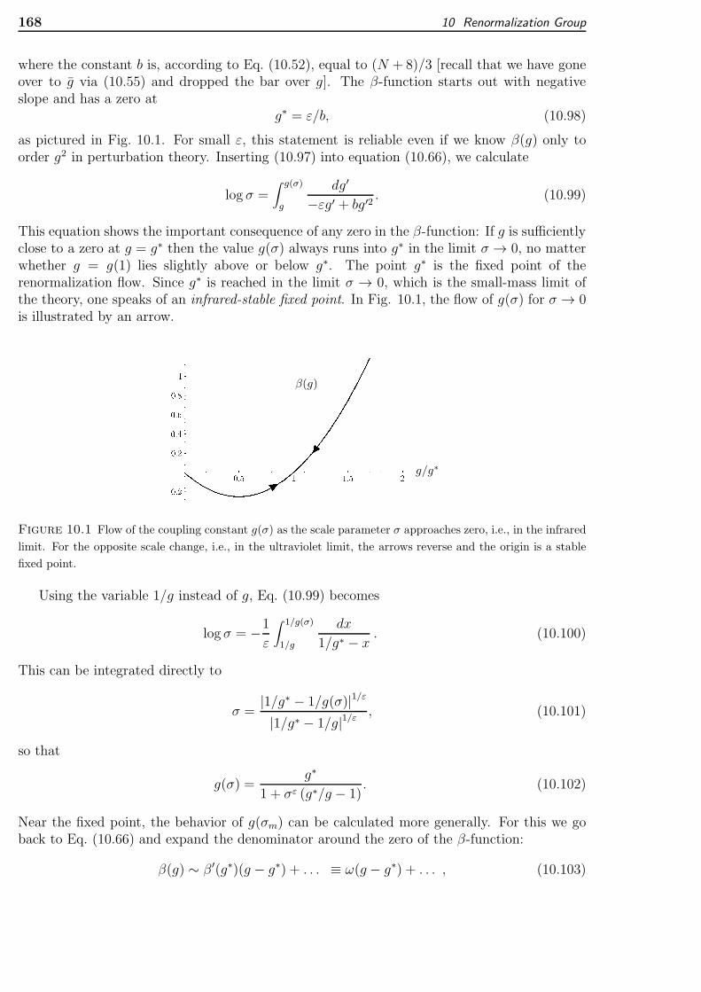
This equation shows the important consequence of any zero in the β-function: If g is sufficientlyclose to a zero at g = g∗ then the value g(σ) always runs into g∗ in the limit σ → 0, no matterwhether g = g(1) lies slightly above or below g∗. The point g∗ is the fixed point of therenormalization flow. Since g∗ is reached in the limit σ → 0, which is the small-mass limit ofthe theory, one speaks of an infrared-stable fixed point. In Fig. 10.1, the flow of g(σ) for σ → 0is illustrated by an arrow.

β(g)

g/g∗

Figure 10.1 Flow of the coupling constant g(σ) as the scale parameter σ approaches zero, i.e., in the infrared

limit. For the opposite scale change, i.e., in the ultraviolet limit, the arrows reverse and the origin is a stable

fixed point.

Using the variable 1/g instead of g, Eq. (10.99) becomes

log σ = −1

ε

∫ 1/g(σ)

1/g

dx

1/g∗ − x. (10.100)

This can be integrated directly to

σ =|1/g∗ − 1/g(σ)|1/ε

|1/g∗ − 1/g|1/ε, (10.101)

so that

g(σ) =g∗

1 + σε (g∗/g − 1). (10.102)

Near the fixed point, the behavior of g(σm) can be calculated more generally. For this we goback to Eq. (10.66) and expand the denominator around the zero of the β-function:

β(g) ∼ β ′(g∗)(g − g∗) + . . . ≡ ω(g − g∗) + . . . , (10.103)

10.6 Effective Energy and Potential 169

where we have introduced the slope of the β-function at the fixed point g∗:

ω ≡ β ′(g∗). (10.104)

This is another critical exponent, as we shall see in Section 10.8. The exponent ω governs theleading corrections to the scaling laws. The sign of ω controls the stability of the fixed point.For an infrared stable fixed point, ω must be positive. Then we obtain from (10.62) an equationfor σ = σm:

log σm =∫ g(σm)

g

dg′

β(g′)∼

1

ωlog

[

g(σm)− g∗

g − g∗

]

, (10.105)

implying the following σm-dependence of g(σm), correct to lowest order in g − g∗:

g(σm)− g∗

g − g∗= σω

m. (10.106)

This agrees with the specific solution (10.102) derived from the β-function (10.97) which hasω = ε.

In general, the β-function may behave in many different ways for larger g. In particular,there may be more zeros to the right of g∗. We can see from Eq. (10.99) that, for positive β,the coupling constant g(σ) will always run towards zero from the right. For negative β, it willrun away from zero to the right.

Note that, in general, the initial coupling g(µ) = g(1) can flow only into the zero which liesin its range of attraction. In the present case this is guaranteed for small ε, if g(1) is sufficientlysmall.

In the limit σ → ∞, we see from Eq. (10.102) that g(σ) tends to zero, which is the trivialzero of the β-function. This happens for any zero with a negative slope of β(g). The limitσ → ∞ corresponds to m2 → ∞, and for this reason such zeros are called ultraviolet stable. Inthis limit g(σ) → 0, γ(g(σ)) → 0, and γm(g(σ)) → 0. Then scaling relation (10.84) impliesthat σm = m/µ, and the correlation functions behave, by (10.86), like those of a free theory:

Γ(n)(ki;m, g, µ)m≈0≈

(

m

µ

)D−n(D/2−1)

Γ(n)(kiµ/m; 0, µ, µ). (10.107)

This is the behavior of a free-field theory where the fields fluctuate in a trivial purely Gaussianway. The zero in β(g) at g = 0 is therefore called the Gaussian or trivial fixed point. In theφ4-theory, the Gaussian fixed point is ultraviolet stable (UV-stable). Since the theory tends form → ∞ against a free theory, one also says that it is ultraviolet free. Note that this is trueonly in less than four dimensions.

In D = 4 dimensions, where ε = 0, the β-function has only one fixed point, the trivialGaussian fixed point at the origin.

10.6 Effective Energy and Potential

The above considerations are useful for deriving the critical properties of a system only in thenormal phase, where T ≥ Tc. If we want to study the system in the phase with spontaneoussymmetry breakdown, which exists for T ≤ Tc, we have to perform a renormalization groupanalysis for the effective energy Γ[Φ] of the system, introduced in Section 5.6, and analyze


its behavior as a function of the mass parameter µ. For this purpose we expand the effectiveenergy in a power series in the field expectations in momentum space Φ(p) as

Γ[Φ;m, g, µ] =∞∑

n=1

1

n!

∫

dDp1(2π)D

. . .dDpn(2π)D

Φ(p1) · · ·Φ(pn)Γ(n)(p1, . . . ,pn;m, g, µ). (10.108)

The coefficients are the proper vertex functions. We have omitted for a moment the term n = 0in this expansion, since it will require extra treatment. Actually, the omission calls for a newnotation for the effective action, but since the reduced sum (10.108) will appear frequently inwhat follows, while the full effective action appears only in a few equations, we prefer keepingthe notation unchanged, and shall instead refer to the full effective action including the n = 0 -term as Γtot[Φ;m, g, µ].

Let us now apply the renormalization group equation (10.29) to each coefficient. Thenwe observe that the factor n in front of γ(g) in Eq. (10.29) can be generated by a functionalderivative with respect to the field expectations Φ(p), replacing

n→∫ dDp

(2π)DΦ(p)

δ

δΦ(p). (10.109)

Then we find immediately the renormalization group equation

[

µ∂µ + β(g)∂g − γ(g)∫

dDp

(2π)DΦ(p)

δ

δΦ(p)+ γm(g)m∂m

]

Γ[Φ(p);m, g, µ] = 0. (10.110)

The addition of the missing n = 0 term will modify this equation as we shall see in the nextsection.

A corresponding equation holds for the effective potential v(Φ). This is defined as thenegative effective energy density at a constant average field Φ(x) ≡ Φ:

v(Φ) = −L−DΓ[Φ;m, g, µ]|Φ(x)≡Φ. (10.111)

Here L is the linear size of the D-dimensional box under consideration. The effective potentialsatisfies the differential equation

[µ∂µ + β(g)∂g − γ(g)Φ∂Φ + γm(g)m∂m] v(Φ;m, g, µ) = 0. (10.112)

Due to its special relevance to physical applications, we solve here only the latter equationalong the lines of Eqs. (10.61)–(10.70). We introduce a running field strength Φ(σ), satisfyingthe differential equation

1

Φ(σ)σd

dσΦ(σ) = −γ(g(σ)), (10.113)

with the initial condition

Φ(1) = Φ. (10.114)

The equation is solved by

Φ(σ)

Φ= exp

{

−∫ σ

1

dσ′

σ′γ(g(σ′))

}

= exp

{

−∫ g(σ)

gdg′

γ(g′)

β(g′)

}

. (10.115)

10.6 Effective Energy and Potential 171

Using this function Φ(σ), the effective potential satisfies the renormalization group equation[analogous to (10.70)]:

v(Φ;m, g, µ) = v(Φ(σ);m(σ), g(σ), µσ). (10.116)

Note that there is no prefactor as in (10.70).Since Γ[Φ] is dimensionless and v(Φ) is related to Γ[Φ] by (10.111), there is a naive scaling

relation analogous to (10.76):

v(Φ;m, g, µ) = σDv(

Φ

σD/2−1;m

σ, g,

µ

σ

)

. (10.117)

Together with (10.116), this gives

v(Φ;m, g, µ) = σDv

(

Φ(σ)

σD/2−1;m(σ)

σ, g(σ), µ

)

. (10.118)

At the mass dependent value σm = m(σm)/µ, we obtain the analog of (10.79) for the effectivepotential

v(Φ;m, g, µ) = σDm v

(

Φ(σm)

σD/2−1m

;µ, g(σm), µ

)

. (10.119)

In the limit m→ 0, where σ → 0, we see from Eq. (10.115) that the field behaves like

Φ(σm)

Φ≈ σ−γ∗

m . (10.120)

The effective potential has therefore the power behavior

v(Φ;m, g, µ)m≈0≈ σD

m v(Φ/σγ∗+D/2−1m ;µ, g∗, µ), (10.121)

where σm is related to t = m2/µ2 by (10.84).For applications to many-body systems below Tc, it is most convenient to consider, instead

of Γ[Φ;m, g, µ], the proper vertex functions in the presence of an external magnetization. Theyare obtained by expanding Γ[Φ;m, g, µ] functionally around Φ(x) ≡ Φ0:

Γ(n)(x1, . . . ,xn; Φ;m, g, µ) ≡δnΓ[Φ;m, g, µ]

δΦ(x1) . . . δΦ(xn)

∣

∣

∣

∣

∣

Φ≡Φ0

. (10.122)

In momentum space, this gives

Γ(n)(k1, . . . ,kn; Φ0;m, g, µ) =∞∑

n′=0

Φn′

0

n′!Γ(n+n′)(k1, . . .kn, 0, . . . , 0;m, g, µ), (10.123)

where the zeros after the arguments k1, . . . ,kn indicate that there are n′ more momentumarguments kn+1, . . . ,kn+n′ which have been set zero since a constant field Φ(x) ≡ Φ0 has aFourier transform Φ(k) ≡ Φ0δ

(D)(k). Thus the renormalization group equation for the propervertex function at a nonzero field, Γ(n)(k1, . . . ,kn; Φ0;m, g, µ), can be obtained from those atzero field Γ(n+n′)(k1, . . . ,kn,kn+1, . . . ,kn+n′;m, g, µ) with the last n′ momenta set equal to zero,i.e., from

[µ∂µ + β(g)∂g − (n+ n′)γ(g) + γm(g)m∂m]

× Γ(n+n′)(k1, . . . ,kn, 0, . . . , 0;m, g, µ) = 0. (10.124)


Inserting this into (10.123), we obtain the renormalization group equation[

µ∂µ + β(g)∂g − γ(g)

(

n + Φ0∂

∂Φ0

)

+ γm(g)m∂m

]

× Γ(n)(k1, . . . ,kn; Φ0, m, g, µ) = 0. (10.125)

When treated as above, this leads to the scaling relation

Γ(n)(ki; Φ0;m, g, µ) = e−n∫

σ

1

dσ′

σ′γ(g(σ′))Γ(n)(ki; Φ0(σ);m(σ), g(σ), µσ). (10.126)

Together with the trivial scaling relation

Γ(n)(ki; Φ0;m, g, µ) = σD−n(D/2−1)Γ(n)(ki/σ; Φ0/σD/2−1;m/σ, g, µ/σ), (10.127)

we find

Γ(n)(ki; Φ0;m, g, µ) = σD−n(D/2−1)e−n∫

σ

1

dσ′

σ′γ(g(σ′))

× Γ(n)(ki/σ; Φ0(σ)/σD/2−1;m(σ)/σ, g(σ), µ). (10.128)

This becomes, at σ = σm of Eq. (10.78),

Γ(n)(ki; Φ0;m, g, µ) = σD−n(D/2−1)m e−n

∫

σm

1

dσ′

σ′γ(g(σ′))

× Γ(n)(ki/σm; Φ0(σm)/σD/2−1m ;µ, g(σm), µ), (10.129)

and thus, near the critical point,

Γ(n)(ki; Φ0;m, g, µ) = n(γ∗ +D/2− 1)Γ(n)(ki/σm; Φ0/σγ∗+D/2−1m ;µ, g∗, µ). (10.130)

10.7 Special Properties of Ground State Energy

When deriving the behavior of the proper vertex functions Γ(n)(k1, . . . ,kn;m, g) under changesof the scale parameter µ, the number n was restricted to positive integer values n ≥ 1. Thevacuum energy contained in Γ(0)(m, g) was omitted from the sum in Eq. (10.108). Indeed, thevacuum energy does not follow the regular renormalization pattern. For the above calculationof the critical exponents, this irregularity is irrelevant. But if we want to calculate amplituderatios (recall the definition in Section 1.2), we have to know the full thermodynamic potentialas the temperature approaches the critical point from above and from below. Then the specialrenormalization properties of the vacuum diagrams can no longer be ignored. The fundamentaldifference between the ground state energies above and below the transition was seen at themean-field level in Eq. (1.43). While the vacuum energy is identically zero above the tran-sition, it behaves like −(T − Tc)

2 below Tc, which is the condensation energy in mean-fieldapproximation.

More subtleties appear when calculating loop corrections. The lowest-order vacuum diagramshows a peculiar feature: with the help of (8.116) and (8.117), we find the full semiclassicaleffective potential at zero average field Φ and coupling constant:

vtot(0;m, 0, µ) =N

2

∫

dDp

(2π)Dlog(p2 +m2)

=N

2

2

D

(m2)D/2

(4π)D/2Γ(1−D/2) =

N

2

m4

µε

1

(4π)2

[

−1

ε+

1

2

(

logm2

4πµ2e−γ−

3

2

)]

+O(ε). (10.131)

10.7 Special Properties of Ground State Energy 173

The pole term at ε = 0 can be removed by adding to the potential a counterterm

vsg ≡N

2

m4

µε

1

(4π)21

ε. (10.132)

To find a finite effective potential order by order in perturbation theory, we must perform theperturbation expansion with an additional term in the initial energy functional, which carriesan additional set of pole terms, to be written collectively as [6, 7]

∆E ≡ −LD m4(µ)

(4π)2g(µ)µǫZv(g(µ), ε), (10.133)

where Zv(g, ε) is the renormalization constant of the vacuum which has an expansion in powersof 1/ε analogous to the other renormalization constants in (10.35)–(10.37):

Zv(g, ε) ≡∞∑

n=1

Zv,n(g)1

εn. (10.134)

The expansion coefficients of Zv up to five loops will be given in Eq. (15.35).The analogy of Zv with the other renormalization constants is not perfect: there is no

constant zero-loop term in Zv. Such a term would be there if we had added to the bare energyfunctional a term −LDm4

BhB/λB with an arbitrary constant hB. Such a term would have atemperature dependence ∝ m4

B ∝ t2 contributing a constant background term to the specificheat near Tc which is needed to describe experiments. Indeed, the specific heat [see the curvesin Fig. 1.1 and their best fit (1.22)] shows a critical power behavior of t superimposed upon asmooth background term. The latter can be fitted by an appropriate constant hB. The sumover the pole terms in Zv, on the other hand, diverges for t → 0 and generates the criticalpower behavior proportional to |t|Dν which, after two derivatives with respect to t, producesthe observed peak in the specific heat C ∝ tDν−2 ∝ |t|−α. This will be seen explicitly on thenext page.

The effective energy of the vacuum is obtained from the sum of all loop diagrams Γ(0)B , plus

the additional term ∆E. The total sum is the renormalized effective energy of the vacuum:

Γ(0) = Γ(0)B +∆E. (10.135)

Now, the bare effective energy at fixed bare quantities is certainly independent of the regular-ization parameter µ, and therefore satisfies trivially the differential equation

µd

dµΓ(0)B

∣

∣

∣

∣

∣

B

= 0. (10.136)

For the renormalized effective energy (10.135), this implies that

µd

dµΓ(0)

∣

∣

∣

∣

∣

B

= µd

dµ∆E

∣

∣

∣

∣

∣

B

. (10.137)

Inserting here the right-hand side of (10.133), this equation can be written as

µd

dµΓ(0)

∣

∣

∣

∣

∣

B

= −LD m4(µ)

(4π)2g(µ)µεγv(g(µ)), (10.138)


with the renormalization group function of the vacuum

γv(g) ≡ − [ε+ β(g, ε)/g − 4γm]Zv(g, ε) + β(g, ε)∂gZv(g, ε). (10.139)

This function depends only on the renormalized coupling constant g as a consequence of therenormalizability of the theory and the minimal subtraction scheme. The derivative on theleft-hand side of (10.137) is converted, via the chain rule, into a sum of differentiations withrespect to the renormalized parameters, as in Eq. (10.21). Thus we obtain for Γ(0)(m, g, µ) therenormalization group equation

[

µ∂

∂µ+ β(m, g, µ)

∂

∂g+ γm(m, g, µ)m

∂

∂m

]

Γ(0)(m, g, µ) = −LD

(4π)2m4(µ)

µεg(µ)γv(g(µ)) . (10.140)

On the right-hand side we have emphasized the µ-dependence of m and g, to avoid confusionwith m = m(1) and g = g(1) defined in (10.61), (10.62). Inserting the expansion (10.134) of Zv

into the right-hand side of (10.140), we find that the differentiations isolate from Zv preciselythe residue of the simple pole term 1/ε, yielding

γv = gZ ′

v,1(g). (10.141)

All higher pole terms cancel, since the functions Zv,n satisfy recursion relations similar to(10.48)–(10.50):

gZ ′

v,n+1(g) = [4γm − β0(g)/g]Zv,n + β0(g)Z′

v,n(g), (10.142)

with β0(g) of Eq. (10.41).The renormalization group equation (10.140) can now be solved to find the renormalized

effective energy of the vacuum [recall (10.119)]:

Γ(0)(m, g, µ) = LDσDm v

(

Φ(σm)

σD/2−1m

;µ, g(σm), µ

)

min

−LD

(4π)2m4h

gµε

∫ σm

1

dσ

σ1+εγv(g(σ))m

4(σ).

(10.143)In the scaling regime, where σm is small and the mass goes to zero like

m(σm) ≈ mσγ∗

m

m , (10.144)

the additional term ∆E in the effective energy of the vacuum in (10.135) is proportional to

∆E ∝ m4σ4γ∗

m−εm ∝ tν(4γ

∗

m−ε)+2 = tDν . (10.145)

Thus it has the same scaling behavior as the incomplete effective potential v(Φ) at Φ = 0 [i.e.,the effective potential without the n = 0 -term in the sum (10.108)], which according to (10.89)and (10.121) behaves like σD

m ∝ tDν . It is also the same as that for the effective potential at anontrivial minimum Φ = Φ0 in the ordered state, as we shall see from (10.167). This will beimportant later in Subsection 10.10.3 when calculating the critical exponent of the specific heatdefined in (1.16). The calculation of the universal ratios of the amplitudes of the specific heatand other quantities depend crucially on the renormalized vacuum energy Γ(0)(m, g, µ) [8].

10.8 Approach to Scaling

In Eq. (10.93), we derived Kadanoff’s scaling law (1.28) from the scaling relation (10.86) forthe two-point proper vertex function. From this, we extracted the critical exponents ν =

10.8 Approach to Scaling 175

1/(2 − 2γ∗m) governing the temperature behavior of the correlation length, and the exponentη = 2γ∗ determining the critical power behavior of the Green function.

In Eq. (10.104), we introduced a further important critical exponent which governs theapproach to the scaling law (10.93) for g → g∗. In order to find this, we expand the right-handside of Eq. (10.79) around g∗ and write

Γ(n)(ki;m, g, µ) = σD−n(D/2−1)m exp

[

−n∫ σm

1dσ′

γ(g(σ′))

σ′

]

Γ(n) (ki/σm, µ, g∗, µ)

×C(n)(ki/σm;µ, g(σm), µ), (10.146)

with the correction factor C(n) given by

C(n)(ki/σm;µ, g(σm), µ) = 1 + [g(σm)− g∗]∂

∂glog Γ(n)(ki/σm;µ, g, µ)

∣

∣

∣

∣

∣

g=g∗

+ . . . . (10.147)

Using Eq. (10.106), the correction factor is rewritten as

C(n)(ki/σm;µ, g(σm), µ) = 1 + (g − g∗)σωm

∂

∂glog Γ(n)(ki/σm;µ, g, µ)

∣

∣

∣

g=g∗+ . . . , (10.148)

where ω is the slope of the β-function at g = g∗, as defined in Eq. (10.104).When approaching the critical point σm → 0, a finite correction to scaling is observed if

∂ log Γ(n)/∂g is at g = g∗ homogenous of degree ω in the variables ki/σm. For the two-pointproper vertex function such a behavior implies the following form of the correction factor

C(2)(k/σm, 1, g∗, 1)

m≈0≈ 1 + const × (g − g∗)σω

m × (|k|/µσm)−ω + . . . . (10.149)

Then

Γ(2)(k;m, g, µ) = σ2m exp

[

−2∫ σm

1dσ′

γ(g(σ′))

σ′

]

Γ(2) (k/σm, µ, g∗, µ)C(2)(k/σm;µ, g(σm), µ)

(10.150)

behaves for t ≈ 0 like

Γ(2)(k;m, g, µ)m≈0≈ |k|2−ηf(|k|/µtν)

1 + (g − g∗)× const ×

(

|k|

µ

)

−ω

+ . . .

.

(10.151)

Thus the correction to scaling is described by the exponent ω which is the slope of the β-function at the fixed point g∗. From the above discussion it is obvious that ω is positive for aninfrared stable fixed point.

The most accurately measured approach to scaling comes from space shuttle experimentson the specific heat in superfluid helium, plotted in Fig. 1.2. The correction factor for thisapproach is obtained from Eq. (10.148) for n = 0 to have the general scaling form

C(0) = 1 + const× σωm = 1 + const× tνω, (10.152)

where we have used (10.84) to express σm in terms of t = T/Tc−1. The exponent νω is usuallycalled ∆ [compare Eq. (1.22)].

At this point one may wonder about the universality of this result since, in principle, othercorrections to scaling might arise from neglected higher powers of the field of higher gradientterms in the energy functional, for example φ6 or φ(∂φ)2. Fortunately, all such terms can beshown to be irrelevant for the value of ω. This is suggested roughly by dimensional considera-tions, and proved by studying the flow of these terms towards the critical limit with the helpof the renormalization group [9].


10.9 Further Critical Exponents

The critical exponents ν, η, ω determine the critical behavior of all observables and the approachto this behavior. Let us derive the scaling relations for several important thermodynamicquantities and correlation functions.

10.9.1 Specific Heat

Consider the specific heat as a function of temperature. The ground state energy above Tc isgiven by the effective potential at zero average field vh(Φ = 0) which, according to (10.89),(10.121), and (10.145), has the scaling behavior

vh(Φ = 0)m≈0≈ σD

m × const. +m4σ4γ∗

m−εm × const. ≈ tDν , (10.153)

the second term coming from the sum of the vacuum diagrams in Eq. (10.145). Forming thesecond derivative with respect to t, we find for the specific heat at constant volume

Ct≈0≈ tD/(2−2γ∗

m)−2 = tDν−2, t > 0. (10.154)

This behavior has been observed experimentally, and the critical exponent has been named α[recall (1.16)]:

Ct≈0≈ t−α; t > 0. (10.155)

Thus we can identify

α = 2−Dν = 2−D/(2− 2γ∗m), (10.156)

showing that the exponent α is directly related to ν, as stated before in the scaling relation(1.32).

10.9.2 Susceptibility

Suppose the system at T > Tc is coupled to a nonzero external source j, which is the gen-eralization of an external magnetic field in magnetic systems [recall Eq. (1.44) and (1.45)].The equilibrium value of the magnetization M ≡ Φ is no longer zero but MB ≡ Φ(j). It isdetermined by the equation of state [the generalization of (1.46)]

j =∂v(Φ)

∂Φ

∣

∣

∣

∣

∣

Φ(j)

. (10.157)

From (10.121) we see that in the vicinity of the critical point

jt≈0≈ σm

D−γ∗−(D/2−1)v′(Φ(j)/σγ∗+D/2−1

m ;µ, g∗, µ), t > 0. (10.158)

The susceptibility is obtained by an additional differentiation with respect to Φ [see Eq. (1.47)]:

χ−1 ≡∂2v

∂Φ2

∣

∣

∣

∣

∣

Φ=Φ(j)

t≈0≈ σm

D−(D−2)σ−2γ∗

m v′′(Φ(j)σ−(D−2)/2−γ∗

m ;µ, g∗, µ), t > 0. (10.159)

For O(N)-symmetric systems above Tc, this equation applies to the invariant part of the sus-ceptibility matrix defined by Eq. (1.12). Below Tc, we must distinguish between longitudinaland transverse susceptibilities. This will be done in Subsection 10.10.5.

10.10 Scaling Relations Below Tc 177

At t = 0 and zero field, one has Φ(j) = 0 and finds

χ−1 ∝ σ2−2γ∗

m = t(2−2γ∗)/(2−2γ∗

m). (10.160)

Experimentally, this critical exponent is called γ [recall (1.17)]:

χ−1 t≈0≈ tγ, t > 0. (10.161)

The critical exponent γ should not be confused with the renormalization group function γ(g)of Eq. (10.26). Comparing (10.161) with (10.160), we identify

γ = 21− γ∗

2− 2γ∗m= ν(2 − η), (10.162)

thus reproducing the scaling relation (1.34).

10.9.3 Critical Magnetization

At the critical point, the proportionality of j and Φ (or ofH andM) is destroyed by fluctuations.Experimentally, one observes a scaling relation [recall (1.20)]

M ≈ B1/δ, t = 0. (10.163)

This can be derived from Eq. (10.158) which shows that a finite effective potential at the criticalpoint, where σm = 0, requires the derivative v′ to behave like some power for small σm = 0:

v′t≈0≈ const.×

(

Φ/σγ∗+D/2−1m

)δ, t > 0. (10.164)

From the proportionality j ∝ σD−γ∗−(D/2−1)

m v′, the power δ which makes j finite in the limitσm → 0 must satisfy

D − γ∗ − (D/2− 1)− [γ∗ + (D/2− 1)] δ = 0. (10.165)

From this we obtain

δ =D + 2− 2γ∗

D − 2 + 2γ∗=D + 2− η

D − 2 + η, (10.166)

which is the scaling relation (1.35).

10.10 Scaling Relations Below Tc

Let us now turn to scaling results below Tc. Since all individual vertex functions in the expansionof the effective energy (10.108) can be calculated for m2 < 0 just as well as for m2 > 0, themain difference lies in v(Φ) not having a minimum at Φ = 0 but at Φ = Φ0 6= 0 for vanishingexternal fields.


10.10.1 Spontaneous Magnetization

Consider first the behavior of the spontaneous magnetization M0 ≡ Φ0 as the temperatureapproaches Tc from below. The equilibrium value of Φ is determined by the minimum of theeffective potential v(Φ). According to (10.121), the minimum must have a constant ratio:

Φ0/σγ∗+D/2−1m = const . (10.167)

Hence, Φ0 depends on m2 and thus on the reduced temperature t as follows:

M0 ≡ Φ0 ∝ σγ∗+D/2−1m = t(γ

∗+D/2−1)/(2−2γ∗

m). (10.168)

Thus we derive the experimentally observable relation [compare (1.19)]

M0 ≡ Φ0 ∝ (−t)β, (10.169)

with the critical exponent

β =γ∗ +D/2− 1

2− 2γ∗m=ν

2(D − 2 + η). (10.170)

This relation agrees with (1.33).

10.10.2 Correlation Length

Consider now the temperature dependent correlation length below Tc. From (10.130) we readoff that the two-point function satisfies

Γ(2)(k; Φ0;m, g, µ)t≈0≈ σ2−2γ∗

m Γ(2)(

k/σm; Φ0/σγ∗+D/2−1m ;µ, g∗, µ

)

, t < 0. (10.171)

As in the previous case above Tc [recall (10.86), (10.87)], this is a function of

k/σm = µ ξ(t)k, (10.172)

with the same temperature behavior as in (10.90). Thus the same critical exponent governsthe divergence of the correlation length below and above Tc.

This above-below equality will now also be derived for the critical exponents α and γ ofspecific heat and susceptibility, respectively. The derivation of their scaling behaviors for t < 0requires keeping track of the change of the average field Φ0 with temperature.

10.10.3 Specific Heat

The exponent α of the specific heat below Tc follows from the Φ0 6= 0 -version of Eq. (10.153)for the effective potential:

vh(Φ0)t≈0≈ σD

mv(

Φ0/σγ∗+D/2−1m , µ, g∗, µ

)

+ const.×m4σ4γ∗

m−εm . (10.173)

Since the temperature change of Φ0 takes place at a constant combination Φ0/σγ∗+D/2−1m [see

Eq. (10.167)], the presence of Φ0 6= 0 can be ignored and we obtain the same result as in(10.153), implying a temperature behavior

v(Φ0) ∝ σDm ≈ tDν . (10.174)

This agrees with the T > Tc -behavior (10.153), leading to the same critical exponent of thespecific heat as in (10.156).

10.10 Scaling Relations Below Tc 179

10.10.4 Susceptibility

Suppose now that an external magnetic field is switched on in the ordered phase. It will causea deviation δΦ ≡ Φ(j) − Φ0 from Φ0. From Eqs. (10.157) and (10.158) we obtain for δΦ thescaling relation

j → σD−(γ∗+D/2−1)m v′((Φ0 + δΦ)/σγ∗+D/2−1

m ;µ, g∗, µ). (10.175)

Expanding this to first order in δΦ gives

δj → δΦσ2−2γ∗

m v′′(Φ0/σγ∗+D/2−1m ;µ, g∗, µ). (10.176)

Since Φ0 changes with t according to (10.169), the last factor is independent of temperature,and the susceptibility χ(t) has the same functional form as in (10.159), exhibiting the samecritical exponent γ as in (10.161).

In O(N)-symmetric systems, this result holds for the longitudinal susceptibility only. Thetransverse susceptibility requires the following separate discussion.

10.10.5 Transverse Susceptibility and Bending Stiffness

Suppose now that the ground state breaks spontaneously an O(N) symmetry of the system.Then the susceptibility decomposes into a longitudinal part and a transverse part, as shownin Eq. (1.14), and these two parts have completely different scaling properties. Since suscep-tibilities are proportional to correlation functions according to (1.15), we extract their scalingproperties from the lowest gradient term in the effective energy Γ[�;m, g, µ] in the deviationof the average field �(x) from the equilibrium value �0. We write bold-face letters for vectorsin O(N) field space. The quadratic term in the deviation δ�(x) ≡ �(x)−�0 has the generalform

Γ[�;m, g, µ] ≈ ∫

dDx δ�(x)Γ(2)(−i∂x;�0;m, g, µ))δ�(x). (10.177)

For smooth field configurations δ�(x), we expand

Γ(2)(−i∂x;�0;m, g, µ) ≈ c1(�0;m, g, µ)− c2(�0;m, g, µ)∂2x. (10.178)

The temperature dependence of the expansion coefficients c1,2(�0;m, g, µ) can be extractedfrom Eq. (10.171) and (10.167). To ensure the existence of a nontrivial term proportional tok2 on the right-hand side of (10.171), we see that

Γ(2)(ki;�0;m, g, µ)t≈0∝ σ2−2γ∗

m + const× σ−2γ∗

m k2. (10.179)

Recalling the dependence (10.89) of σm on t = m2/µ2, and the relation (10.94) for the criticalexponent η, we obtain, for smooth field configurations, the temperature dependence of theleading terms in the effective energy

Γ(2)[�;m, g, µ] t≈0∝∫

dDx{

t(2−η)ν�2(x) + const× t−ην [∂x�(x)]2} . (10.180)

For an O(N)-symmetric system, the order field can be decomposed into size and directionas �(x) = Φ(x)n(x) (10.181)


which brings the effective energy for small and smooth deviations δΦ(x) and δn(x) ≡ n(x)−n0

from the average ordered configurations to the form as

Γ(2)[�;m, g, µ] t≈0∝∫

dDx(

t(2−η)ν{

Φ20 + [δΦ(x)]2

}

+ const×t−ην{

[∂xδΦ(x)]2+Φ2

0 [∂xδn(x)]2})

.

(10.182)

In O(2)-symmetric systems, the order field has two components, and can be replaced by acomplex field Φ(x) = eiθ(x)Φ0(x) with a real Φ0(x). Then the last term in (10.182) has the form

const×∫

dDxt−ηνΦ20 [∂xδθ(x)]

2 . (10.183)

In both gradient terms we can, of course, omit the deviation symbols δ. The directional devia-tion field δn(x) possesses only a gradient term, and describes long-range (massless) excitationswhose existence is ensured by the Nambu-Goldstone theorem stated after Eq. (1.50).

From the coefficients of the quadratic terms we extract the scaling behavior of the longitu-dinal and tranverse correlation functions in momentum space:

GcL(k) ∝[

t(2−η)ν + const× t−ηνk2]

−1, (10.184)

GcT (k) ∝[

const× t−ηνΦ20k

2]

−1. (10.185)

The longitudinal and tranverse susceptibilities are proportional to these [recall Eq. (1.15)].Their critical behavior is given by

χ−1cL(0) ∝ t(2−η)ν (10.186)

k−2 χ−1c T (k) ∝

∂

∂k2χ−1cL(k) ∝ t−ηνΦ2

0. (10.187)

Recalling the temperature dependence (10.169) of Φ0, and using the scaling relation for theaverage field Φ0 in Eq. (10.169), the second relation becomes

k−2 χ−1cT (k) ∝

∂

∂k2χ−1cL(k) ∝ t(D−2)ν . (10.188)

Comparison of the last term in Eq. (10.182) with (1.110) shows that the prefactor suppliesus with the temperature behavior of the bending stiffness of the directional field n(x) near thecritical point. In superfluid helium, this is by definition proportional to the experimentallymeasured superfluid density ρs [recall Eq. (1.122)]. The bending stiffness, or the superfluiddensity, are therefore proportional to those in (10.188), and we obtain the temperature behaviorof the superfluid density

ρs ∝ t(D−2)ν . (10.189)

The experimental verification of this scaling behavior was described in Chapter 1, the crucialplots being shown in Fig. ??.

10.10.6 Widom’s Relation

Finally it is worth noticing that Eq. (10.158) corresponds exactly to Widom’s scaling relation(1.26). That relation can be differentiated with respect to M to yield the magnetic equation ofstate

B = t3−αM−1−1/βψ′(t/M1/β), (10.190)

10.11 Comparison of Scaling Relations with Experiment 181

which may also be written asB

M δ= f

(

t

M1/β

)

(10.191)

with some function f(x). This is easily proven with the help of Griffith’s scaling relationδ = −1 + (2− α)/β [recall (1.29)]. In terms of the variables of our field theory, the equation ofstate (10.191) may be rewritten as

j = tδβ(

t

Φ1/β

)−δβ

f(

t

Φ1/β

)

= tδβg(

Φ

tβ

)

, (10.192)

where g(x) is some other function. By comparing this with (10.158), we see that

δβ = [D − γ∗ − (D/2− 1)]1

2− 2γ∗m=ν

2(D + 2− η), (10.193)

which is in agreement with (10.166), (10.170), or (1.33) and (1.35).

10.11 Comparison of Scaling Relations with Experiment

For a comparison with experiment, we may pick three sets of critical data and extract the valuesof η, ν, and ω. The remaining critical exponents can then be found from the scaling relations(1.32)–(1.35).

As an example take the magnetic system CrBr3 where one measures

β ≈ 0.368, δ ≈ 4.3, γ ≈ 1.215. (10.194)

Inserting these into Widom’s scaling relation [recall (1.30)]

β = γ/(δ − 1) , (10.195)

we see that the relation is satisfied excellently. Inserting δ into the relation

η =D + 2− (D − 2)δ

δ + 1, (10.196)

we find for D = 3η ≈ 0.132, (10.197)

and from the relation ν = γ/(2− η) [recall (1.34)]:

ν ≈ 0.65. (10.198)

10.12 Critical Values g*, η , ν, and ω in Powers of ε

Let us now calculate explicitly the critical properties of the O(N)-symmetric φ4-theory in thetwo-loop approximation. In Eq. (10.56) we gave the β-function

β(g) = −εg +N + 8

3g2 −

3N + 14

3g3. (10.199)

In D = 4 dimensions, β(g) starts with g2, and the only IR-stable fixed point lies at g∗ = 0.Thus the massless φ4-theory behaves asymptotically as a free theory. From Eqs. (10.52) and


(10.53) we see that the anomalous dimensions γ and γm are zero for g∗ = 0. Hence the criticalexponents in Eqs. (10.88), (10.94), and (10.104) possess the mean field values for D = 4:

η = 0 , ν = 1/2 , ω = 0 . (10.200)

In D = 4 − ε dimensions, the equation β(g∗) = 0 for the fixed point has the nontrivialsolution

g∗ =3

N + 8ε+

9(3N + 14)

(N + 8)3ε2 + . . . . (10.201)

If this expansion is inserted into the g-expansions (10.57)–(10.58), we obtain for the criticalexponents ν and η the ε-expansions:

η = 2γ∗(ε,N) =N + 2

2(N + 8)2ε2 + . . . , (10.202)

ν =1

2− 2γ∗m(ε,N)=

1

2+

N + 2

4(N + 8)ε+

(N + 2)(N2 + 23N + 60)

8(N + 8)3ε2 + . . . . (10.203)

The critical exponent ω governing the approach to scaling is found from the derivative of theβ-function (10.56) at g = g∗ [recall (10.104)]:

ω = β ′∗(ε,N) = ε− 33N + 14

(N + 8)2ε2 + . . . . (10.204)

All ε-expansions are independent of the choice of the coupling constant. The critical expo-nents depend via ε and N only on the dimension of space and order parameter space. This isa manifestation of the universality of phase transitions, which states that the critical behaviordepends only on the type of interaction, its symmetry, and the space dimensionality.

Let us compare the above ε-expansion with the experimental critical exponents in Section10.11. The expansion can be used only for infinitesimal ε. For applications to three dimensionswe have to evaluate them at ε = 1, which cannot be done by simply inserting this large ε-value, since the series diverge. Let us ignore this problem for the moment, deferring a properresummation until Chapters 16, 19, and 20. Inserting ε = 1, and estimating the reliability ofthe result from the size of the last term in each series, we calculate for N = 0, 1, 2, 3,∞ :

ν = 12+ 1

16ε+ 15

512ε2 + . . . = 303

512+ . . . ≈ 0.5918± 0.0293, N = 0,

ν = 12+ 1

12ε+ 7

162ε2 + . . . = 203

324+ . . . ≈ 0.6265± 0.0432, N = 1,

ν = 12+ 1

10ε+ 11

200ε2 + . . . = 131

200+ . . . ≈ 0.6550± 0.0550, N = 2,

ν = 12+ 5

44ε+ 345

5324ε2 + . . . = 903

1331+ . . . ≈ 0.6874± 0.0648, N = 3,

ν = 12+ 1

4ε+ 1

8ε2 + . . . = 7

8+ . . . ≈ 0.8750± 0.1250, N = ∞.

(10.205)

The other critical exponents are

η = 164

≈ 0.016, N = 0,

η = 154

≈ 0.019, N = 1,

η = 150

≈ 0.02, N = 2,

η = 5242

≈ 0.021, N = 3,

η = 0, N = ∞,

(10.206)

10.13 Several Coupling Constants 183

and

ω = ε− 1727ε2 = 10

27≈ 0.3704± 0.6296, N = 0,

ω = ε− 1727ε2 = 10

27≈ 0.3704± 0.6296, N = 1,

ω = ε− 35ε2 = 2

5≈ 0.4± 0.6, N = 2,

ω = ε− 69121ε2 = 52

121≈ 0.4298± 0.5702, N = 3,

ω = ε = 1, N = ∞.

(10.207)

The ε-expansion for ν has decreasing contributions from higher orders. The value up to orderε2 is ν ≈ 0.627, and agrees reasonably with the experimental value ν ≈ 0.65 of Eq. (10.198).

The expansions for η contain only one term, so no convergence can be judged. The agreementwith experiment is nevertheless reasonable. The value to order ε2 at ε = 1 is η ≈ 0.019 which,via the scaling relation ν = γ/(2 − η), leads to the exponent γ ≈ 1.287, quite close to theexperimental value γ = 1.215 in Eq. (10.194).

The expansion for ω are obviously useless since the errors are too large.

If we attempt to calculate critical exponents to higher order than ε2 by inserting ε = 1 into theexpansions, we observe that the agreement becomes worse since the series diverge. The roughagreement for ν and ǫ up to order ε2 is a consequence of the asymptotic convergence of the series.In Chapter 16, we shall see how high-precision estimates can still be extracted from asymptoticseries. The reader who is curious to see how the direct evaluation of the series becomes worsewith higher orders in ε may anticipate the five-loop expansions from Eqs. (17.13)–(17.15) andinsert ε = 1 into these.

For a judgment of the reliability of all numbers (10.205)–(10.207), we refer the reader to themost accurate currently available critical exponents in Tables 20.2 and ??.

10.13 Several Coupling Constants

For fields with more than one component, several φ4-couplings are possible which may allbecome simultaneously relevant in four dimensions. This was discussed in detail in Chapter6. For each coupling constant, there exists a β-function and there may be two or more fixedpoints. The stability of the fixed points depends on N and channels the flow in the space ofthe coupling constants. It can be shown in general [10] that the O(N)-symmetric fixed pointis the only stable one for N ≤ 4−O(ε).

In order to have only a single wave function renormalization constant for the N field com-ponents φα, the following condition has to be fulfilled:

Γ(2)αβ(k) ∼ Γ(2)(k) δαβ . (10.208)

This property is guaranteed for all theories which are symmetric under reflection φα → −φα

and under permutations of the N field indices α. The same symmetry ensures that Γ(4) is, to allorders in perturbation theory, a linear combination of the tensors specifying the φ4-couplings.For two tensors T

(1)αβγδ and T

(2)αβγδ, this condition reads

Γ(4)αβγδ ∼ Γ

(4)1 T

(1)αβγδ + Γ

(4)2 T

(2)αβγδ . (10.209)


If the conditions (10.208) and (10.209) are satisfied, we can find four scalar renormalizationconstants ZA (A = φ,m2, g1, g2) relating the bare mass mB and the two coupling constants giBto the corresponding physical parameters by

m2B =

Zm2

Zφm2; giB = µε Zgi

(Zφ)2 gi for i = 1, 2 . (10.210)

The renormalization group functions are introduced in the usual way:

βi(g1, g2) = µ∂µgi|g1B ,g2B ,mB ,ε = µ∂µgi∣

∣

∣

B, (10.211)

γ(g1, g2) = µ∂µ logZ1/2φ |g1B ,g2B,mB ,ε = µ∂µ logZ

1/2φ

∣

∣

∣

B, (10.212)

γm(g1, g2) = µ∂µ logm|g1B,g2B ,mB,ε = µ∂µ logm∣

∣

∣

B. (10.213)

We have written Eqs. (10.211)–(10.213) by analogy with Eqs. (10.30)–(10.33). Since the renor-malization constants depend on g1 and g2, the functions g1 and g2 are implicitly given by

giB = µεZgiZ−2φ gi = giB(µ, g1(µ), g2(µ)). (10.214)

The derivatives ∂µg1 and ∂µg2 follow therefore from the two equations

∂giB∂µ

+∂giB∂g1

∂g1∂µ

+∂giB∂g2

∂g2∂µ

= 0 for i = 1, 2. (10.215)

Using ∂µgiB = ε giB/µ, we find

∂ log giB∂g1

β1 +∂ log giB∂g2

β2 = −ε for i = 1, 2. (10.216)

The renormalization group function γ(g1, g2) is given by

γ(g1, g2) =β1(g1, g2)

2

∂ logZφ

∂g1+β2(g1, g2)

2

∂ logZφ

∂g2, (10.217)

while γm is obtained from the equation

γm(g1, g2) = −β1(g1, g2)

2

∂ logZm2

∂g1−β2(g1, g2)

2

∂ logZm2

∂g2+ γ(g1, g2). (10.218)

Extracting the regular terms of Eqs. (10.216)–(10.218), we find the analog of Eqs. (10.43)–(10.46) for the case with two coupling constants:

β1 = −εg1 + g1 (g1∂g1Zg1,1 + g2∂g2Zg1,1 + 4 γ) ,

β2 = −εg2 + g2 (g2∂g2Zg2,1 + g1∂g1Zg2,1 + 4 γ) ,

γ = − 1

2g1∂g1Zφ,1 − 1

2g2∂g2Zφ,1,

γm = 1

2g1∂g1Zm2,1 + 1

2g2∂g2Zm2,1 + γ. (10.219)

The stability of the fixed points can be examined using the critical exponents ω1, ω2, whichare the eigenvalues of the matrix ∂βi/∂gj . They should be positive for an infrared stable fixedpoint. An example for a system with two coupling constants will be treated in Chapter 18.

10.14 Ultraviolet versus Infrared Properties 185

10.14 Ultraviolet versus Infrared Properties

Some remarks may be useful concerning the special role of ultraviolet divergences in criticalphenomena. In three dimensions, φ4-theories are superrenormalizable and possess finite cor-relation functions after only a few subtractions. So one may wonder about the relevance ofultraviolet divergences to critical phenomena, in particular, since the system at short distancesis not supposed to be represented by the field theory. The explanation of this apparent paradoxis the following. Consider some real physical system with a microstructure, such as a lattice, ata temperature very close to the critical temperature at which the correlation length ξ extendsover many lattice spacings. There the correlation functions have three regimes. At very longdistances x ≫ ξ, they fall off exponentially like e−x/ξ. For distances much larger than thelattice spacing but much smaller than the correlation length, they behave like a power in x.At the critical temperature, this power behavior extends all the way out to infinite distances.In the third regime, where distances are of the order of the lattice spacing, the behavior isnonuniversal and depends crucially on the composition of the material. Nothing can be saidabout this regime on the basis of field-theoretic studies.

Let us compare these behaviors of correlation functions of real systems with the behaviorsfound in the present φ4 field theories. Here we can also distinguish three regimes. The third,unphysical regime, lies now at distances which are shorter than the inverse cutoff Λ of thetheory. In this regime, the perturbation theory has unphysical singularities, first discussed byLandau, that are completely irrelevant to the critical phenomena to be explained. At lengthscales much shorter than the correlation length, but much longer than 1/Λ, the correlationfunctions show power behavior, from which we can extract the critical exponents of the fieldtheory and compare them with experiments made in the above lattice system. In field theory,this is the so-called short-distance behavior. Its properties are governed by the ultravioletdivergences. At the critical point, the short-distance behavior extends all the way to infinity.This is the reason why ultraviolet divergences are relevant for the understanding of long-distancephenomena observed in many-body systems near the critical point, that are independent of themicrostructure.

Notes and References

Excellent reviews are found inE. Brezin, J.C. Le Guillou, J. Zinn-Justin, in Phase Transitions and Critical Phenomena, Vol.6,edited by C. Domb and M.S. Green, Academic Press, New York, 1976;K.G. Wilson, J. Kogut, Phys. Rep. 12, 75 (1974),and in the textbook byD.J. Amit, Field Theory, the Renormalization Group and Critical Phenomena, McGraw-Hill,1978,and the other textbooks cited in Notes and References of Chapter 1.

The individual citations in the text refer to:

[1] C.G. Callan, Phys. Rev. D 2, 1541 (1970);K. Symanzik, Commun. Math. Phys. 18, 227 (1970).

[2] S. Weinberg, Phys. Rev. 118, 838 (1960).


[3] G.’t Hooft, Nucl. Phys. B 61, 455 (1973).

[4] J.C. Collins, A.J. MacFarlane, Phys. Rev. D 10, 1201 (1974).

[5] G.’t Hooft in The Whys of Subnuclear Physics, Ed. A. Zichichi, Proceedings, Erice 1977,Plenum, New York 1979.See alsoN.N. Khuri, Phys. Rev. D 23, 2285 (1981).

[6] B. Kastening, Phys. Lett. B 283, 287 (1992).See alsoM. Bando, T. Kugo, N. Maekawa and H. Nakano, Phys. Lett. B 301, 83 (1993).

[7] B. Kastening, Phys. Rev. D 54, 3965 (1996); Phys. Rev. D 57, 3567 (1998).

[8] S.A. Larin, M. Monnigmann, M. Strosser and V. Dohm (cond-mat/9805028);S.A. Larin, and V. Dohm, Nucl.Phys. B 540, 654 (1999) (cond-mat/9806103);H. Kleinert, B. Van den Bossche, Phys. Rev. E 63, 056113 (2001) (cond-mat/0011329)

[9] See the review article by E. Brezin et al. and textbook by D. Amit cited above.

[10] E. Brezin, J.C. Le Guillou, J. Zinn-Justin, Phys. Rev. B 10, 893 (1974).

RenormalizationGroup - Freie...

Documents

Transcript of RenormalizationGroup - Freie...