Renormalization Group Equations - uni-jena.degies/LectureNotes/PoS/LastR...RG flow in Theory Space...
72
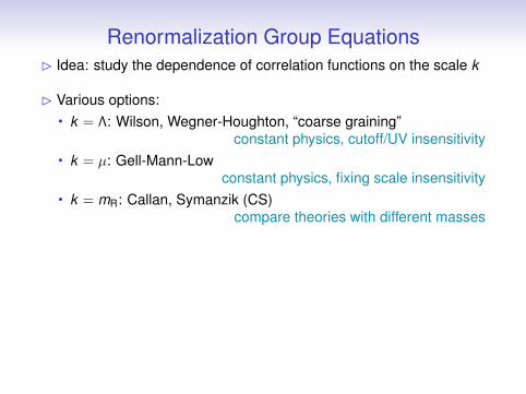
Renormalization Group Equations ✄ Idea: study the dependence of correlation functions on the scale k ✄ Various options: • k =Λ: Wilson, Wegner-Houghton, “coarse graining” constant physics, cutoff/UV insensitivity • k = μ: Gell-Mann-Low constant physics, fixing scale insensitivity • k = m R : Callan, Symanzik (CS) compare theories with different masses
Transcript of Renormalization Group Equations - uni-jena.degies/LectureNotes/PoS/LastR...RG flow in Theory Space...
Renormalization Group Equations� Idea: study the dependence of correlation functions on the scale k
� Various options:• k = Λ: Wilson, Wegner-Houghton, “coarse graining”
constant physics, cutoff/UV insensitivity• k = µ: Gell-Mann-Low
constant physics, fixing scale insensitivity• k = mR: Callan, Symanzik (CS)
compare theories with different masses
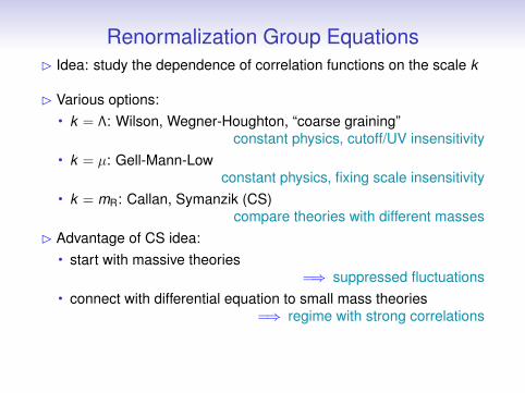
Renormalization Group Equations� Idea: study the dependence of correlation functions on the scale k
� Various options:• k = Λ: Wilson, Wegner-Houghton, “coarse graining”
constant physics, cutoff/UV insensitivity• k = µ: Gell-Mann-Low
constant physics, fixing scale insensitivity• k = mR: Callan, Symanzik (CS)
compare theories with different masses� Advantage of CS idea:
• start with massive theories=⇒ suppressed fluctuations
• connect with differential equation to small mass theories=⇒ regime with strong correlations
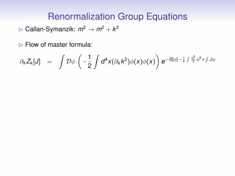
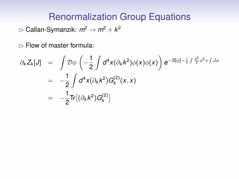
Renormalization Group Equations� Callan-Symanzik: m2 → m2 + k2
� Flow of master formula:
∂k Zk [J] =
∫Dφ
(−1
2
∫d4x(∂k k2)φ(x)φ(x)
)e−S[φ]− 1
2
∫ k22 φ
2+∫
Jφ
Renormalization Group Equations� Callan-Symanzik: m2 → m2 + k2
� Flow of master formula:
∂k Zk [J] =
∫Dφ
(−1
2
∫d4x(∂k k2)φ(x)φ(x)
)e−S[φ]− 1
2
∫ k22 φ
2+∫
Jφ
= −12
∫d4x(∂k k2)G(2)
k (x , x)
= −12
Tr[(∂k k2)G(2)
k
]
Renormalization Group Equations� Callan-Symanzik: m2 → m2 + k2
� Flow of master formula:
∂k Zk [J] =
∫Dφ
(−1
2
∫d4x(∂k k2)φ(x)φ(x)
)e−S[φ]− 1
2
∫ k22 φ
2+∫
Jφ
= −12
∫d4x(∂k k2)G(2)
k (x , x)
= −12
Tr[(∂k k2)G(2)
k
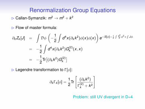
]� Legendre transformation to Γ[φ]:
∂k Γk [φ] =12
Tr
[(∂k k2)
Γ(2)k + k2
]
Problem: still UV divergent in D=4
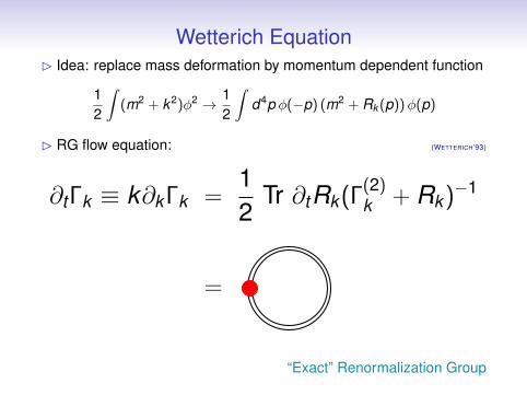
Wetterich Equation� Idea: replace mass deformation by momentum dependent function
12
∫(m2 + k2)φ2 → 1
2
∫d4p φ(−p) (m2 + Rk (p))φ(p)
� RG flow equation: (WETTERICH’93)
∂tΓk ≡ k∂kΓk =12
Tr ∂tRk(Γ(2)k + Rk)−1
=
“Exact” Renormalization Group

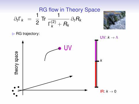
RG flow in Theory Space
∂tΓk =12
Tr1
Γ(2)k + Rk
∂tRk
� RG trajectory: Γk =Λ = SmicroUV: k → Λ
k
IR: k → 0
RG flow in Theory Space
∂tΓk =12
Tr1
Γ(2)k + Rk
∂tRk
� RG trajectory:UV: k → Λ
k
IR: k → 0

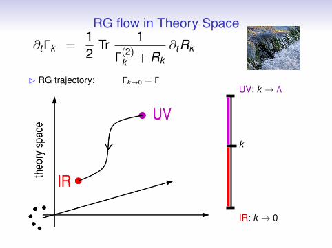
RG flow in Theory Space
∂tΓk =12
Tr1
Γ(2)k + Rk
∂tRk
� RG trajectory:UV: k → Λ
k
IR: k → 0

RG flow in Theory Space
∂tΓk =12
Tr1
Γ(2)k + Rk
∂tRk
� RG trajectory: Γk→0 = ΓUV: k → Λ
k
IR: k → 0
RG flow in Theory Space
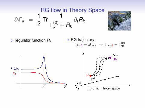
∂tΓk =12
Tr1
Γ(2)k + Rk
∂tRk
� regulator function Rk � RG trajectory:Γk=Λ = Sbare → Γk=0 = Γ1PI
eff

RG flow in Theory Space
∂tΓk =12
Tr1
Γ(2)k + Rk
∂tRk
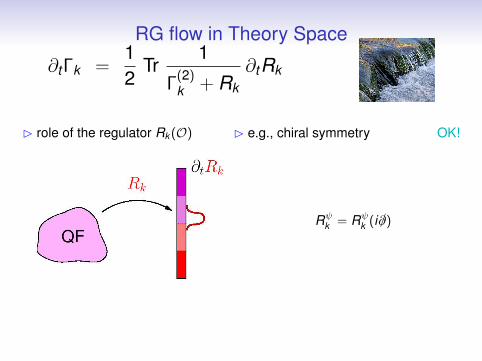
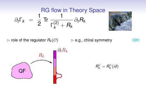
� role of the regulator Rk (O) � e.g., chiral symmetry OK!
Rψk = Rψ
k (i /∂)

RG flow in Theory Space
∂tΓk =12
Tr1
Γ(2)k + Rk
∂tRk
� role of the regulator Rk (O) � e.g., chiral symmetry OK!
Rψk = Rψ
k (i /∂)
RG flow in Theory Space
∂tΓk =12
Tr1
Γ(2)k + Rk
∂tRk
� role of the regulator Rk (O) � e.g., chiral symmetry OK!
Rψk = Rψ
k (i /∂)
RG flow in Theory Space
∂tΓk =12
Tr1
Γ(2)k + Rk
∂tRk
� role of the regulator Rk (O) � e.g., chiral symmetry OK!
Rψk = Rψ
k (i /∂)
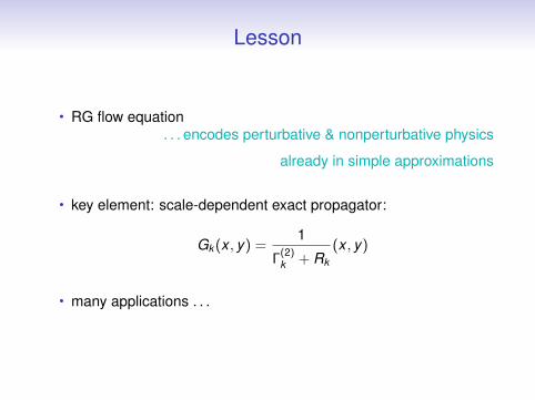
Lesson
• RG flow equation. . . exact equation
• RG flow equation (+ b.c.). . . can serve as definition of QFT
• Wilsonian momentum-shell integration. . . treats physics scale by scale
• key element: scale-dependent exact propagator:
Gk (x , y) =1
Γ(2)k + Rk
(x , y)
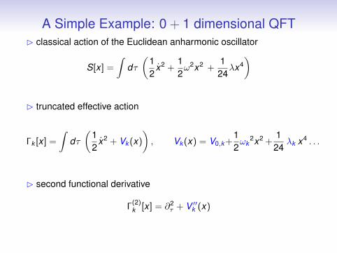
A Simple Example: 0 + 1 dimensional QFT� classical action of the Euclidean anharmonic oscillator
S[x ] =
∫dτ(
12
x2 +12ω2x2 +
124λx4
)
� truncated effective action
Γk [x ] =
∫dτ(
12
x2 + Vk (x)
), Vk (x) = V0,k +
12ωk
2x2 +1
24λk x4 . . .
� second functional derivative
Γ(2)k [x ] = ∂2
τ + V ′′k (x)
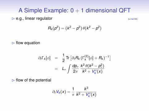
A Simple Example: 0 + 1 dimensional QFT� e.g., linear regulator (LITIM’00)
Rk (p2) = (k2 − p2) θ(k2 − p2)
� flow equation
∂t Γk [φ] =12
Tr[∂tRk (Γ
(2)k [φ] + Rk )−1]
= Lτ∫
dpτ2π
k2 θ(k2 − p2τ )
k2 + V ′′k (x)
� flow of the potential
∂tVk (x) =1π
k3
k2 + V ′′k (x)
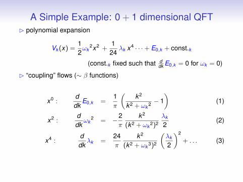
A Simple Example: 0 + 1 dimensional QFT� polynomial expansion
Vk (x) =12ωk
2x2 +124
λk x4 · · ·+ E0,k + const.k
(const.k fixed such that ddk E0,k = 0 for ωk = 0)
� “coupling” flows (∼ β functions)
x0 :ddk
E0,k =1π
(k2
k2 + ωk2 − 1
)(1)
x2 :ddkωk
2 = −2π
k2
(k2 + ωk2)2
λk
2(2)
x4 :ddkλk =
24π
k2
(k2 + ωk3)2
(λk
2
)2
+ . . . (3)
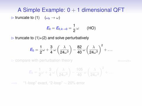
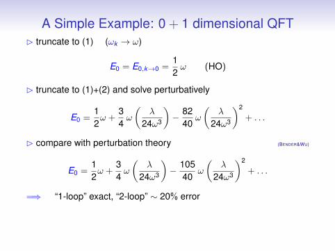
A Simple Example: 0 + 1 dimensional QFT� truncate to (1) (ωk → ω)
E0 = E0,k→0 =12ω (HO)
� truncate to (1)+(2) and solve perturbatively
E0 =12ω +
34ω
(λ
24ω3
)− 82
40ω
(λ
24ω3
)2
+ . . .
� compare with perturbation theory (BENDER&WU)
E0 =12ω +
34ω
(λ
24ω3
)− 105
40ω
(λ
24ω3
)2
+ . . .
=⇒ “1-loop” exact, “2-loop” ∼ 20% error
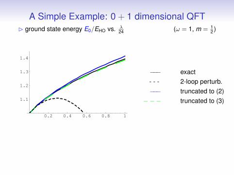
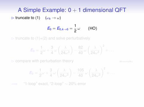
A Simple Example: 0 + 1 dimensional QFT
0.2 0.4 0.6 0.8 1
1.1
1.2
1.3
1.4
� ground state energy E0/EHO vs. λ24 (ω = 1, m = 1
2 )
−−− exact- - - 2-loop perturb.−−− truncated to (2)
−−− truncated to (3)
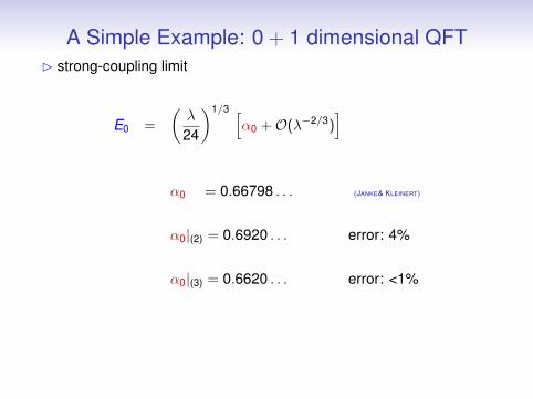
A Simple Example: 0 + 1 dimensional QFT� strong-coupling limit
E0 =
(λ
24
)1/3 [α0 +O(λ−2/3)
]
α0 = 0.66798 . . . (JANKE& KLEINERT)
α0|(2) = 0.6920 . . . error: 4%
α0|(3) = 0.6620 . . . error: <1%
Lesson
• RG flow equation. . . encodes perturbative & nonperturbative physics
already in simple approximations
• key element: scale-dependent exact propagator:
Gk (x , y) =1
Γ(2)k + Rk
(x , y)
• many applications . . .
RG flow in Theory Space
∂tΓk =12
Tr1
Γ(2)k + Rk
∂tRk
� RG trajectory: Γk =Λ = SmicroUV: k → Λ
k
IR: k → 0

RG flow in Theory Space
∂tΓk =12
Tr1
Γ(2)k + Rk
∂tRk
� RG trajectory:UV: k → Λ
k
IR: k → 0

RG flow in Theory Space
∂tΓk =12
Tr1
Γ(2)k + Rk
∂tRk
� RG trajectory:UV: k → Λ
k
IR: k → 0
RG flow in Theory Space
∂tΓk =12
Tr1
Γ(2)k + Rk
∂tRk
� RG trajectory: Γk→0 = ΓUV: k → Λ
k
IR: k → 0
RG flow in Theory Space
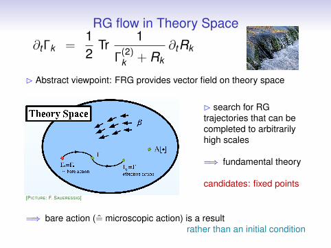
∂tΓk =12
Tr1
Γ(2)k + Rk
∂tRk
� Abstract viewpoint: FRG provides vector field on theory space
� search for RGtrajectories that can becompleted to arbitrarilyhigh scales
=⇒ fundamental theory
candidates: fixed points[PICTURE: F. SAUERESSIG]
=⇒ bare action (= microscopic action) is a resultrather than an initial condition
Quantum field theory←→ gravity� Problem of Physics?
• expected typical scale of QG effects: MPlanck ∼ 1019GeV
• early/late universe cosmology ?
• astrophysical singularities ?
• hierarchy problems(gauge hierarchy, cosmological constant & coincidence problem)
Minimum requirements: compatibility with observed physics
• existence of semiclassical GR regime
• D = 4 = DRG, cr
• compatibility with observed matter content of the universe
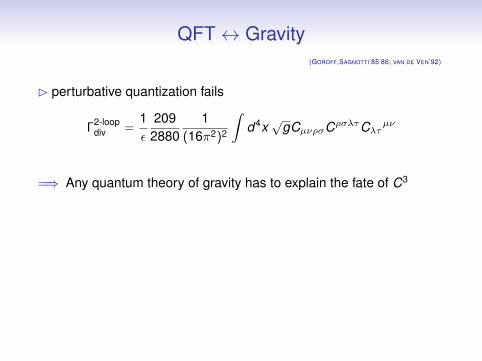
QFT↔ Gravity(GOROFF,SAGNOTTI’85’86; VAN DE VEN’92)
� perturbative quantization fails
Γ2-loopdiv =
1ε
2092880
1(16π2)2
∫d4x√
gCµνρσCρσλτCλτµν
=⇒ Any quantum theory of gravity has to explain the fate of C3
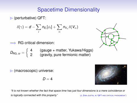
Spacetime Dimensionality� (perturbative) QFT:
δ(γ) = d −∑
i
nEi [φi ] +∑α
nVαδ(Vα)
=⇒ RG critical dimension:
DRG, cr =
{4 (gauge + matter, Yukawa/Higgs)2 (gravity, pure fermionic matter)
� (macroscopic) universe:
D = 4
“It is not known whether the fact that space time has just four dimensions is a mere coincidence or
is logically connected with this property.” (J. ZINN-JUSTIN, IN “QFT AND CRITICAL PHENOMENA”)
Quantizing Gravity
“I know of only one promising approach to this problem . . . ”
(S. WEINBERG, IN “CRITICAL PHENOMENA FOR FIELD THEORISTS” (1976))
Asymptotic Safety
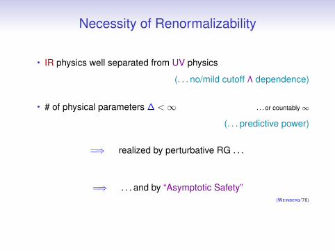
Necessity of Renormalizability
• IR physics well separated from UV physics
(. . . no/mild cutoff Λ dependence)
• # of physical parameters ∆ <∞ . . . or countably∞
(. . . predictive power)
=⇒ realized by perturbative RG . . .
=⇒ . . . and by “Asymptotic Safety”(WEINBERG’76)
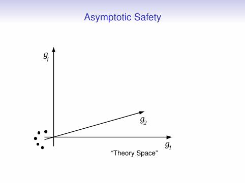
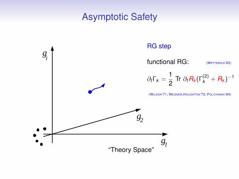
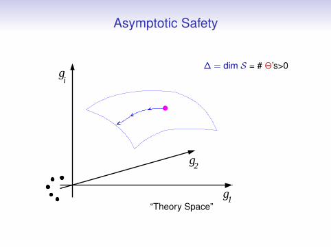
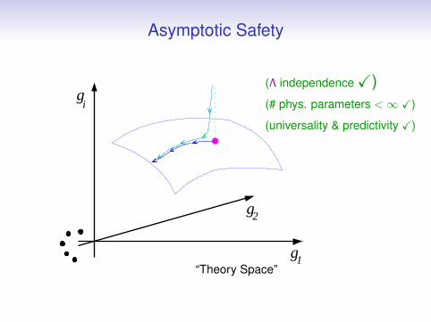
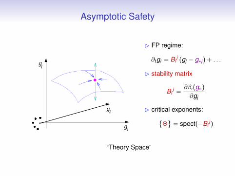
Asymptotic Safety
“Theory Space”g
g
g
1
2
i
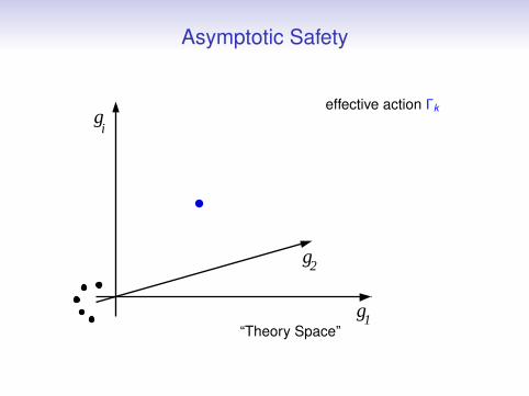
Asymptotic Safety
“Theory Space”g
g
g
1
2
i
effective action Γk
Asymptotic Safety
“Theory Space”g
g
g
1
2
i
RG step
functional RG: (WETTERICH’93)
∂t Γk =12
Tr ∂tRk (Γ(2)k + Rk )−1
(WILSON’71; WEGNER,HOUGHTON’73; POLCHINSKI’84)
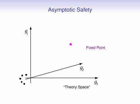
Asymptotic Safety
“Theory Space”g
g
g
1
2
i
Fixed Point
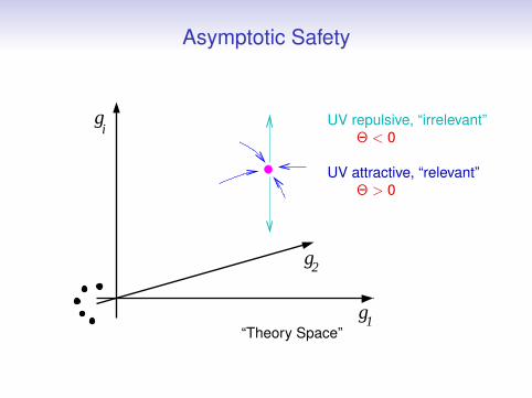
Asymptotic Safety
“Theory Space”g
g
g
1
2
iUV repulsive, “irrelevant”
Θ < 0
UV attractive, “relevant”Θ > 0
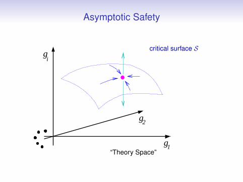
Asymptotic Safety
“Theory Space”g
g
g
1
2
i
critical surface S
Asymptotic Safety
“Theory Space”g
g
g
1
2
i
∆ = dim S = # Θ’s>0
Asymptotic Safety
“Theory Space”g
g
g
1
2
i
(Λ independence X)(# phys. parameters <∞ X)
(universality & predictivity X)
Asymptotic Safety
“Theory Space”
g
g
g
1
2
i
� FP regime:
∂tgi = Bij (gj − g∗j ) + . . .
� stability matrix
Bij =
∂βi (g∗)∂gj
� critical exponents:{Θ}
= spect(−Bij )
Mechanisms of Asymptotic Safety
Dimensional Balancing
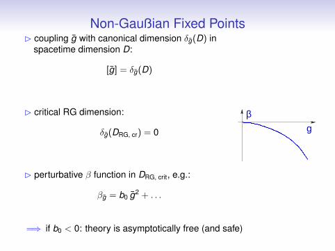
Non-Gaußian Fixed Points� coupling g with canonical dimension δg(D) in
spacetime dimension D:
[g] = δg(D)
� critical RG dimension:
δg(DRG, cr) = 0
� perturbative β function in DRG, crit, e.g.:
βg = b0 g2 + . . .
βg
=⇒ if b0 < 0: theory is asymptotically free (and safe)
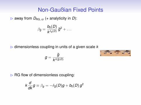
Non-Gaußian Fixed Points� away from DRG, cr (+ analyticity in D):
βg =b0(D)
kδg(D)g2 + . . .
� dimensionless coupling in units of a given scale k
g =g
kδ(g;D)
� RG flow of dimensionless coupling:
kddk
g ≡ βg = −δg(D)g + b0(D) g2
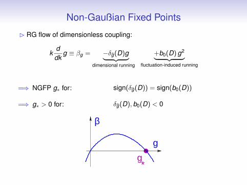
Non-Gaußian Fixed Points
� RG flow of dimensionless coupling:
kddk
g ≡ βg = −δg(D)g︸ ︷︷ ︸dimensional running
+b0(D) g2︸ ︷︷ ︸fluctuation-induced running
=⇒ NGFP g∗ for:
=⇒ g∗ > 0 for:
sign(δg(D)) = sign(b0(D))
δg(D),b0(D) < 0
β
g
g*
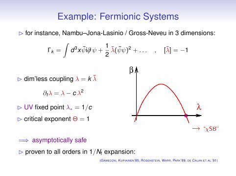
Example: Fermionic Systems
� for instance, Nambu–Jona-Lasinio / Gross-Neveu in 3 dimensions:
Γk =
∫d3xψi∂/ψ +
12λ(ψψ)2 + . . . , [λ] = −1
� dim’less coupling λ = k λ
∂tλ = λ− c λ2
� UV fixed point λ∗ = 1/c
� critical exponent Θ = 1
=⇒ asymptotically safe
� proven to all orders in 1/Nf expansion:(GAWEDZKI, KUPIAINEN’85; ROSENSTEIN, WARR, PARK’89; DE CALAN ET AL.’91)
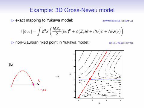
Example: 3D Gross-Neveu model
� exact mapping to Yukawa model: (STRATONOVICH’58,HUBBARD’59)
Γ[ψ, σ] =
∫d3x
(NfZσ
2(∂σ)2 + ψ(Zψ i∂/+ i hσ)ψ + NfU(σ)
)� non-Gaußian fixed point in Yukawa model: (BRAUN,HG,SCHERER’10)
→
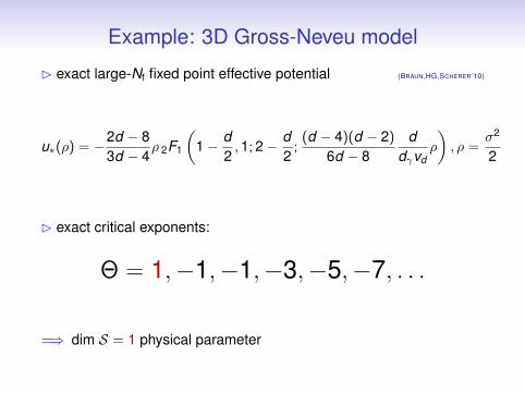
Example: 3D Gross-Neveu model
� exact large-Nf fixed point effective potential (BRAUN,HG,SCHERER’10)
u∗(ρ) = −2d − 83d − 4
ρ 2F1
(1− d
2,1; 2− d
2;
(d − 4)(d − 2)
6d − 8d
dγvdρ
), ρ =
σ2
2
� exact critical exponents:
Θ = 1,−1,−1,−3,−5,−7, . . .
=⇒ dim S = 1 physical parameter
Example: 3D Gross-Neveu model
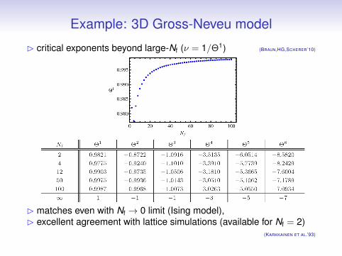
� critical exponents beyond large-Nf (ν = 1/Θ1) (BRAUN,HG,SCHERER’10)
� matches even with Nf → 0 limit (Ising model),� excellent agreement with lattice simulations (available for Nf = 2)
(KARKKAINEN ET AL.’93)
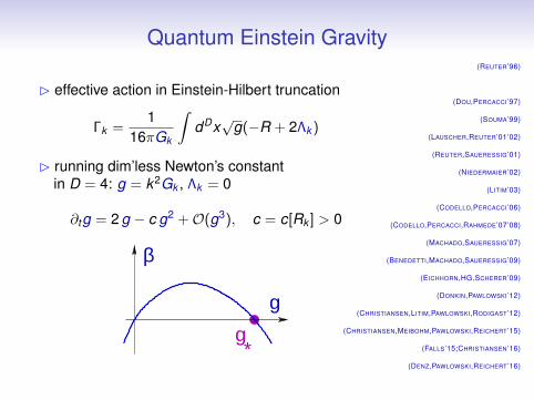
Quantum Einstein Gravity
� effective action in Einstein-Hilbert truncation
Γk =1
16πGk
∫dDx√
g(−R + 2Λk )
� running dim’less Newton’s constantin D = 4: g = k2Gk , Λk = 0
∂tg = 2 g − c g2 +O(g3), c = c[Rk ] > 0
β
g
g*
(REUTER’96)
(DOU,PERCACCI’97)
(SOUMA’99)
(LAUSCHER,REUTER’01’02)
(REUTER,SAUERESSIG’01)
(NIEDERMAIER’02)
(LITIM’03)
(CODELLO,PERCACCI’06)
(CODELLO,PERCACCI,RAHMEDE’07’08)
(MACHADO,SAUERESSIG’07)
(BENEDETTI,MACHADO,SAUERESSIG’09)
(EICHHORN,HG,SCHERER’09)
(DONKIN,PAWLOWSKI’12)
(CHRISTIANSEN,LITIM,PAWLOWSKI,RODIGAST’12)
(CHRISTIANSEN,MEIBOHM,PAWLOWSKI,REICHERT’15)
(FALLS’15;CHRISTIANSEN’16)
(DENZ,PAWLOWSKI,REICHERT’16)
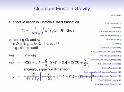
Quantum Einstein Gravity
� effective action in Einstein-Hilbert truncation
Γk =1
16πGk
∫dDx√
g(−R + 2Λk )
� running Gk and Λkin D = 4: g = k2Gk , λ = Λk/k2
e.g., sharp cutoff
∂tg = (2 + η)g
∂tλ = −2(2− η)λ− gπ
[5 ln[1− 2λ]− 2ζ(3) +
52η
]anomalous graviton dimension:
η = − 2g6π + 5g
[18
1− 2λ+ 5 ln(1− 2λ)− ζ(2) + 6
]
(REUTER’96)
(DOU,PERCACCI’97)
(SOUMA’99)
(LAUSCHER,REUTER’01’02)
(REUTER,SAUERESSIG’01)
(NIEDERMAIER’02)
(LITIM’03)
(CODELLO,PERCACCI’06)
(CODELLO,PERCACCI,RAHMEDE’07’08)
(MACHADO,SAUERESSIG’07)
(BENEDETTI,MACHADO,SAUERESSIG’09)
(EICHHORN,HG,SCHERER’09)
(DONKIN,PAWLOWSKI’12)
(CHRISTIANSEN,LITIM,PAWLOWSKI,RODIGAST’12)
(CHRISTIANSEN,MEIBOHM,PAWLOWSKI,REICHERT’15)
(FALLS’15;CHRISTIANSEN’16)
(DENZ,PAWLOWSKI,REICHERT’16)
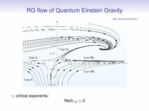
RG flow of Quantum Einstein Gravity(REUTER,SAUERESSIG’01)
� critical exponents:ReΘ1,2 ' 2

From Quantum to Classical Gravity(HG,KNORR,LIPPOLDT’15)
� RG trajectoriesinterconnecting the transplanckian and classical regimes exist
� : physical trajectory:
gλ|k→"today" ' +3× 10−122
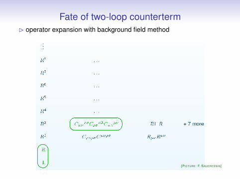
Fate of two-loop counterterm� operator expansion with background field method
[PICTURE: F. SAUERESSIG]
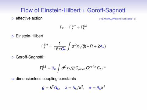
Flow of Einstein-Hilbert + Goroff-Sagnotti� effective action (HG,KNORR,LIPPOLDT,SAUERESSIG’16)
Γk = ΓEHk + ΓGS
k
� Einstein-Hilbert
ΓEHk =
116πGk
∫dDx√
g(−R + 2Λk )
� Goroff-Sagnotti:
ΓGSk = σk
∫dDx√
g CµνρσCρσλτCλτµν
� dimensionless coupling constants
g = k2Gk , λ = Λk/k2, σ = σk k2
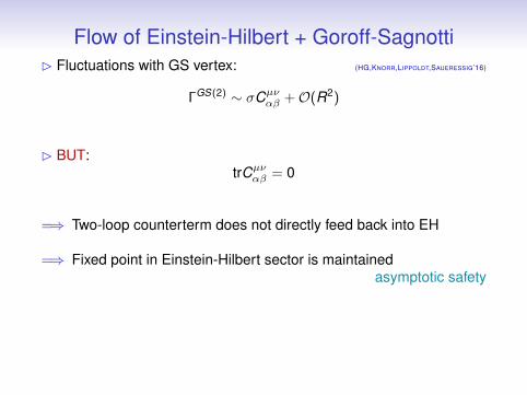
Flow of Einstein-Hilbert + Goroff-Sagnotti� Fluctuations with GS vertex: (HG,KNORR,LIPPOLDT,SAUERESSIG’16)
ΓGS(2) ∼ σCµναβ +O(R2)
� BUT:trCµν
αβ = 0
=⇒ Two-loop counterterm does not directly feed back into EH
=⇒ Fixed point in Einstein-Hilbert sector is maintainedasymptotic safety
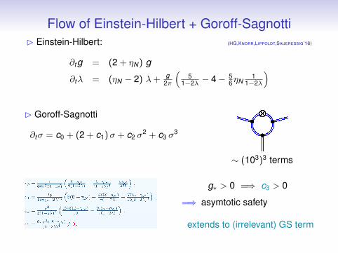
Flow of Einstein-Hilbert + Goroff-Sagnotti� Einstein-Hilbert: (HG,KNORR,LIPPOLDT,SAUERESSIG’16)
∂tg = (2 + ηN) g
∂tλ = (ηN − 2) λ+ g2π
(5
1−2λ − 4− 56ηN
11−2λ
)
� Goroff-Sagnotti
∂tσ = c0 + (2 + c1)σ + c2 σ2 + c3 σ
3
∼ (103)3 terms
g∗ > 0 =⇒ c3 > 0
=⇒ asymtotic safety
extends to (irrelevant) GS term
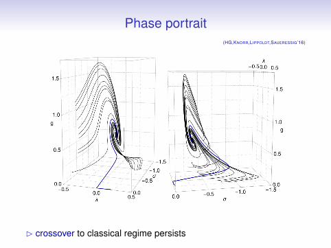
Phase portrait(HG,KNORR,LIPPOLDT,SAUERESSIG’16)
� crossover to classical regime persists
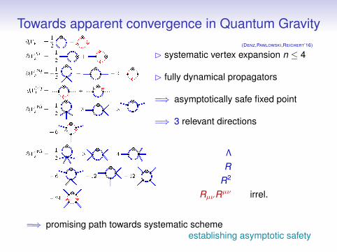
Towards apparent convergence in Quantum Gravity(DENZ,PAWLOWSKI,REICHERT’16)
� systematic vertex expansion n ≤ 4
� fully dynamical propagators
=⇒ asymptotically safe fixed point
=⇒ 3 relevant directions
Λ
RR2
RµνRµν irrel.
=⇒ promising path towards systematic schemeestablishing asymptotic safety
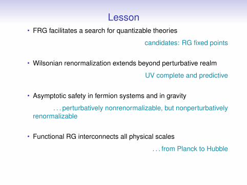
Lesson• FRG facilitates a search for quantizable theories
candidates: RG fixed points
• Wilsonian renormalization extends beyond perturbative realm
UV complete and predictive
• Asymptotic safety in fermion systems and in gravity
. . . perturbatively nonrenormalizable, but nonperturbativelyrenormalizable
• Functional RG interconnects all physical scales
. . . from Planck to Hubble
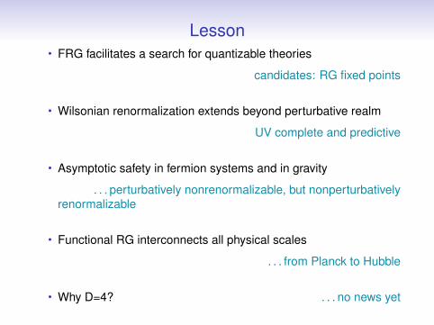
• Why D=4? . . . no news yet
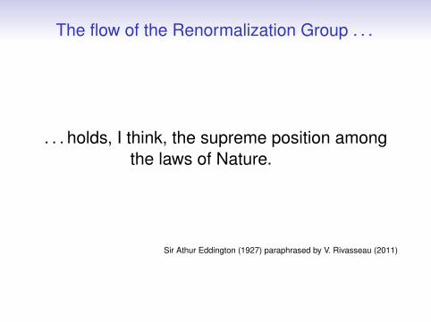
The flow of the Renormalization Group . . .
. . . holds, I think, the supreme position amongthe laws of Nature.
Sir Athur Eddington (1927) paraphrased by V. Rivasseau (2011)
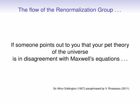
The flow of the Renormalization Group . . .
If someone points out to you that your pet theoryof the universe
is in disagreement with Maxwell’s equations . . .
Sir Athur Eddington (1927) paraphrased by V. Rivasseau (2011)
The flow of the Renormalization Group . . .
. . . then so much the worsefor Maxwell’s equations.
Sir Athur Eddington (1927) paraphrased by V. Rivasseau (2011)
The flow of the Renormalization Group . . .
If it is found to be contradicted by observation. . .
Sir Athur Eddington (1927) paraphrased by V. Rivasseau (2011)
The flow of the Renormalization Group . . .
. . . well, these experimentalistsdo bungle things sometimes.
Sir Athur Eddington (1927) paraphrased by V. Rivasseau (2011)
The flow of the Renormalization Group . . .
But if your theoryis found to be against
the flow of the renormalization group . . .
Sir Athur Eddington (1927) paraphrased by V. Rivasseau (2011)
The flow of the Renormalization Group . . .
I can give you no hope;there is nothing for it
but to collapse in deepest humiliation.
Sir Athur Eddington (1927) paraphrased by V. Rivasseau (2011)


![BIOELECTRO- MAGNETISM - Bioelectromagnetism · Generation of bioelectric signal V. m [mV] 200. 400. 800. 1000-100-50. 0. 50. Time [ms] K + Na + K + K + K + K + K + K + K + K + K +](https://static.fdocument.org/doc/165x107/5ad27ef17f8b9a72118d34d0/bioelectro-magnetism-bi-of-bioelectric-signal-v-m-mv-200-400-800-1000-100-50.jpg)

![AUTARQUIA ASSOCIADA À UNIVERSIDADE DE SÃO PAULO … · fundamentais dos elementos TR, de seus íons TR 3+ [2] e valores dos raios iônicos dos íons TR 3+[5], dados em pm 9 Tabela](https://static.fdocument.org/doc/165x107/5e313e5d011e67436d3c887f/autarquia-associada-universidade-de-sfo-paulo-fundamentais-dos-elementos-tr.jpg)