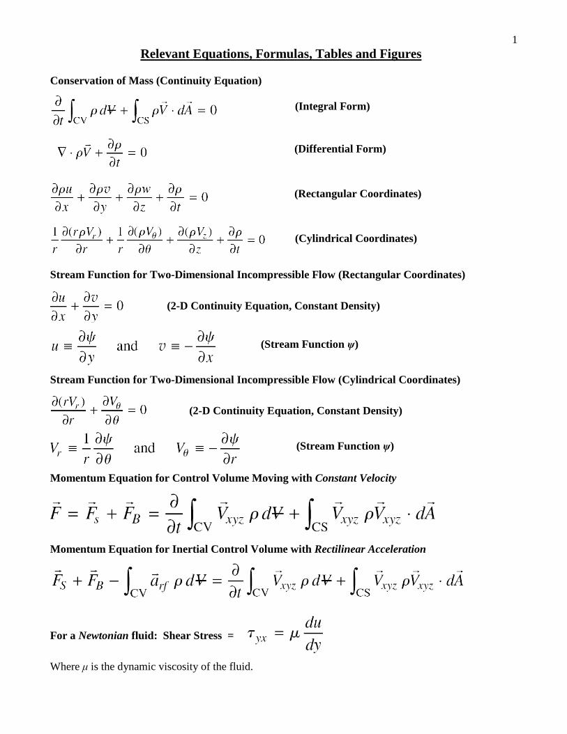
1 Relevant Equations, Formulas, Tables and Figures

Conservation of Mass (Continuity Equation)

(Integral Form)

(Differential Form)

(Rectangular Coordinates)

(Cylindrical Coordinates)

Stream Function for Two-Dimensional Incompressible Flow (Rectangular Coordinates) (2-D Continuity Equation, Constant Density)

(Stream Function ψ)

Stream Function for Two-Dimensional Incompressible Flow (Cylindrical Coordinates) (2-D Continuity Equation, Constant Density)

(Stream Function ψ)

Momentum Equation for Control Volume Moving with Constant Velocity

Momentum Equation for Inertial Control Volume with Rectilinear Acceleration

For a Newtonian fluid: Shear Stress = Where μ is the dynamic viscosity of the fluid.

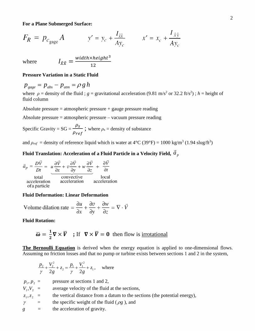
2 For a Plane Submerged Surface:

where 𝐼𝐼𝑥𝑥�𝑥𝑥� = 𝑤𝑤𝑤𝑤𝑤𝑤𝑤𝑤ℎ×ℎ𝑒𝑒𝑤𝑤𝑒𝑒ℎ𝑤𝑤3

12

Pressure Variation in a Static Fluid

hgppp atmabsgage ρ=−= where ρ = density of the fluid ; g = gravitational acceleration (9.81 m/s2 or 32.2 ft/s2) ; h = height of fluid column Absolute pressure = atmospheric pressure + gauge pressure reading

Absolute pressure = atmospheric pressure – vacuum pressure reading

Specific Gravity = SG = 𝜌𝜌𝑠𝑠𝜌𝜌𝑟𝑟𝑟𝑟𝑟𝑟

; where ρs = density of substance

and ρref = density of reference liquid which is water at 4°C (39°F) = 1000 kg/m3 (1.94 slug/ft3)

Fluid Translation: Acceleration of a Fluid Particle in a Velocity Field, pa

Fluid Deformation: Linear Deformation

Fluid Rotation: 𝝎𝝎� = 𝟏𝟏

𝟐𝟐𝛁𝛁 × 𝑽𝑽� ; If 𝛁𝛁× 𝑽𝑽� = 𝟎𝟎 then flow is irrotational

The Bernoulli Equation is derived when the energy equation is applied to one-dimensional flows. Assuming no friction losses and that no pump or turbine exists between sections 1 and 2 in the system,

1

211

2

222

22z

gVpz

gVp

++=++γγ

, where

21 , pp = pressure at sections 1 and 2,

21 ,VV = average velocity of the fluid at the sections,

21 , zz = the vertical distance from a datum to the sections (the potential energy), γ = the specific weight of the fluid ( gρ ), and g = the acceleration of gravity.

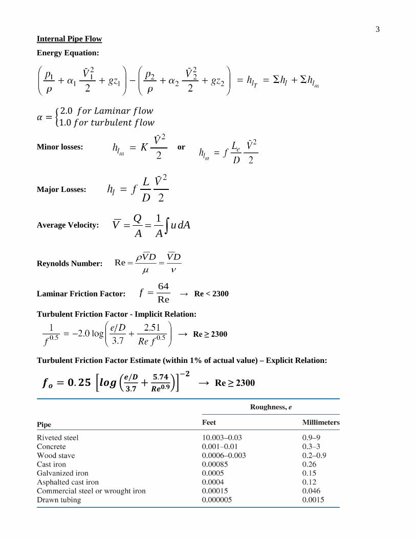
3 Internal Pipe Flow

Energy Equation:

𝛼𝛼 = �2.0 𝑓𝑓𝑓𝑓𝑓𝑓 𝐿𝐿𝐿𝐿𝐿𝐿𝐿𝐿𝐿𝐿𝐿𝐿𝑓𝑓 𝑓𝑓𝑓𝑓𝑓𝑓𝑓𝑓1.0 𝑓𝑓𝑓𝑓𝑓𝑓 𝑡𝑡𝑡𝑡𝑓𝑓𝑡𝑡𝑡𝑡𝑓𝑓𝑡𝑡𝐿𝐿𝑡𝑡 𝑓𝑓𝑓𝑓𝑓𝑓𝑓𝑓

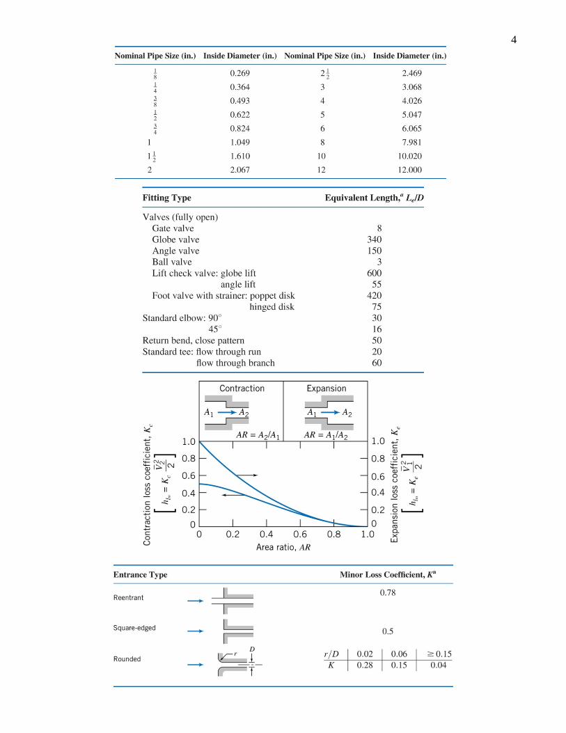
Minor losses: or

Major Losses:

Average Velocity:

Reynolds Number: νµ

ρ DVDV==Re

Laminar Friction Factor: Re64

=f → Re < 2300

Turbulent Friction Factor - Implicit Relation:

→ Re ≥ 2300

Turbulent Friction Factor Estimate (within 1% of actual value) – Explicit Relation:

𝒇𝒇𝒐𝒐 = 𝟎𝟎.𝟐𝟐𝟐𝟐 �𝒍𝒍𝒐𝒐𝒍𝒍 �𝒆𝒆/𝑫𝑫𝟑𝟑.𝟕𝟕

+ 𝟐𝟐.𝟕𝟕𝟕𝟕𝑹𝑹𝒆𝒆𝟎𝟎.𝟗𝟗��

−𝟐𝟐 → Re ≥ 2300

∫== dAuAA

QV 1

4

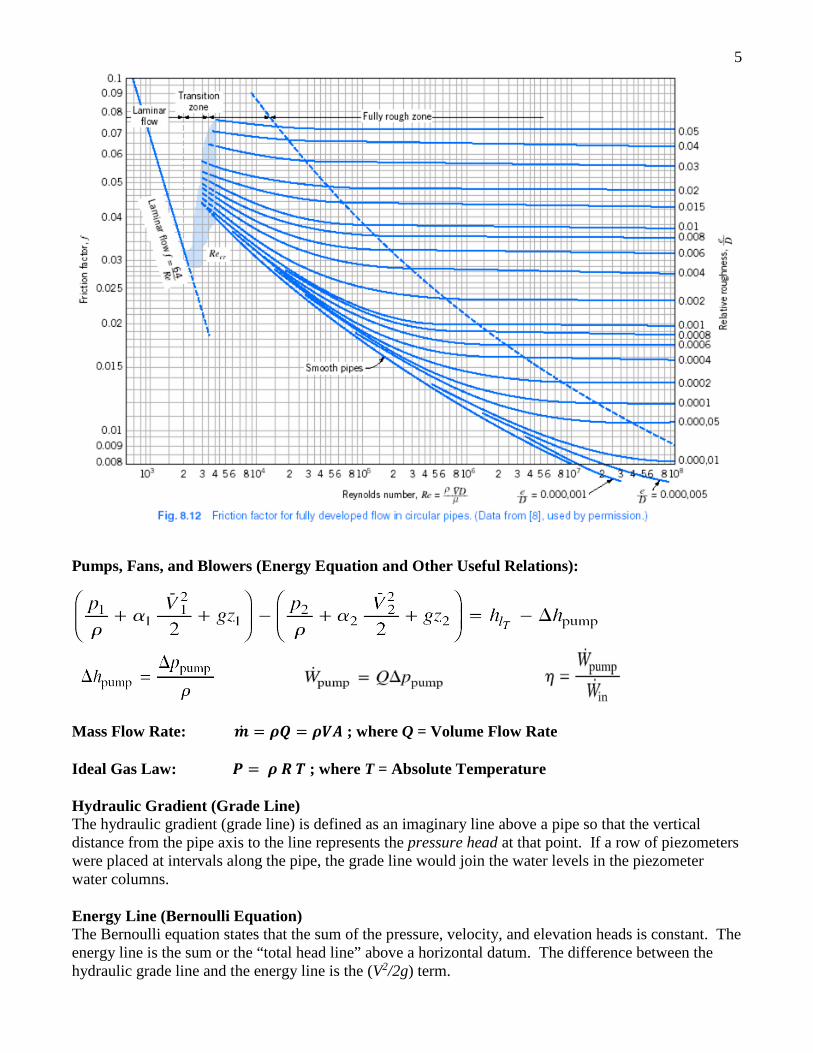
5

Pumps, Fans, and Blowers (Energy Equation and Other Useful Relations):

Mass Flow Rate: �̇�𝒎 = 𝝆𝝆𝝆𝝆 = 𝝆𝝆𝑽𝑽𝝆𝝆 ; where Q = Volume Flow Rate

Ideal Gas Law: 𝑷𝑷 = 𝝆𝝆 𝑹𝑹 𝑻𝑻 ; where T = Absolute Temperature

Hydraulic Gradient (Grade Line) The hydraulic gradient (grade line) is defined as an imaginary line above a pipe so that the vertical distance from the pipe axis to the line represents the pressure head at that point. If a row of piezometers were placed at intervals along the pipe, the grade line would join the water levels in the piezometer water columns. Energy Line (Bernoulli Equation) The Bernoulli equation states that the sum of the pressure, velocity, and elevation heads is constant. The energy line is the sum or the “total head line” above a horizontal datum. The difference between the hydraulic grade line and the energy line is the (V2/2g) term.

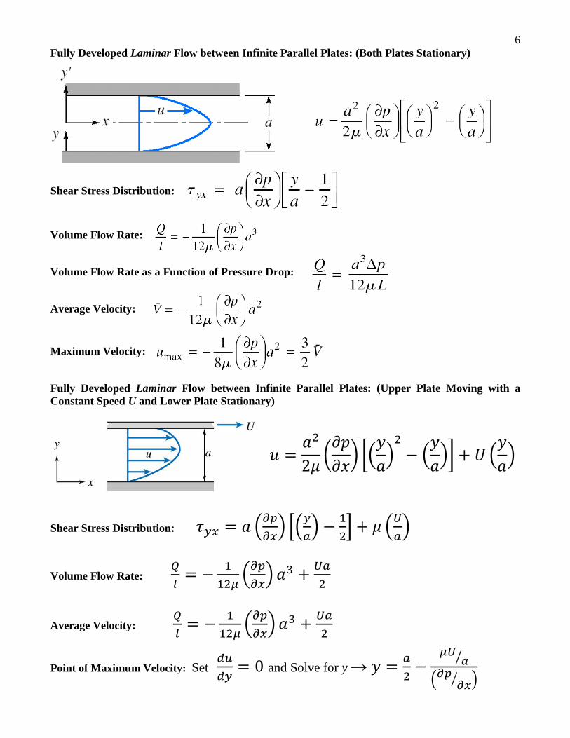
6 Fully Developed Laminar Flow between Infinite Parallel Plates: (Both Plates Stationary)

Shear Stress Distribution: Volume Flow Rate: Volume Flow Rate as a Function of Pressure Drop: Average Velocity:

Maximum Velocity: Fully Developed Laminar Flow between Infinite Parallel Plates: (Upper Plate Moving with a Constant Speed U and Lower Plate Stationary)

𝑡𝑡 =𝐿𝐿2

2𝜇𝜇 �𝜕𝜕𝜕𝜕𝜕𝜕𝜕𝜕� ��

𝑦𝑦𝐿𝐿�

2− �

𝑦𝑦𝐿𝐿�� + 𝑈𝑈 �

𝑦𝑦𝐿𝐿�

Shear Stress Distribution: 𝜏𝜏𝑦𝑦𝑥𝑥 = 𝐿𝐿 �𝜕𝜕𝜕𝜕𝜕𝜕𝑥𝑥� ��𝑦𝑦

𝑎𝑎� − 1

2� + 𝜇𝜇 �𝑈𝑈

𝑎𝑎�

Volume Flow Rate: 𝑄𝑄𝑙𝑙

= − 112𝜇𝜇

�𝜕𝜕𝜕𝜕𝜕𝜕𝑥𝑥� 𝐿𝐿3 + 𝑈𝑈𝑎𝑎

2

Average Velocity: 𝑄𝑄𝑙𝑙

= − 112𝜇𝜇

�𝜕𝜕𝜕𝜕𝜕𝜕𝑥𝑥� 𝐿𝐿3 + 𝑈𝑈𝑎𝑎

2

Point of Maximum Velocity: Set 𝑤𝑤𝑑𝑑𝑤𝑤𝑦𝑦

= 0 and Solve for y → 𝑦𝑦 = 𝑎𝑎2−

𝜇𝜇𝑈𝑈𝑎𝑎�

�𝜕𝜕𝜕𝜕 𝜕𝜕𝑥𝑥� �

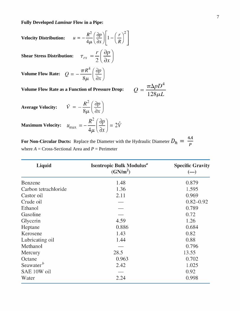
7 Fully Developed Laminar Flow in a Pipe: Velocity Distribution:

Shear Stress Distribution:

Volume Flow Rate: Volume Flow Rate as a Function of Pressure Drop:

Average Velocity:

Maximum Velocity:

For Non-Circular Ducts: Replace the Diameter with the Hydraulic Diameter 𝐷𝐷ℎ = 4𝐴𝐴𝑃𝑃

where A = Cross-Sectional Area and P = Perimeter

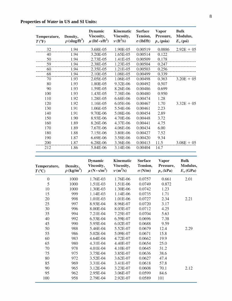
8 Properties of Water in US and SI Units:

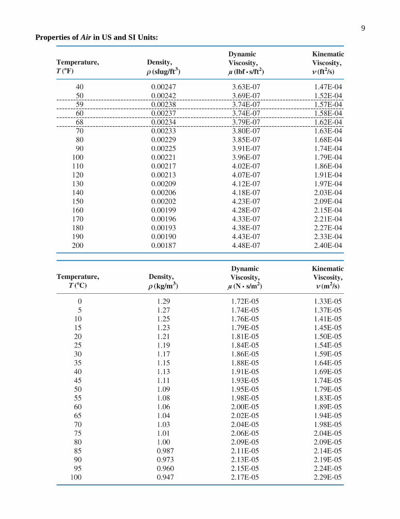
9 Properties of Air in US and SI Units:

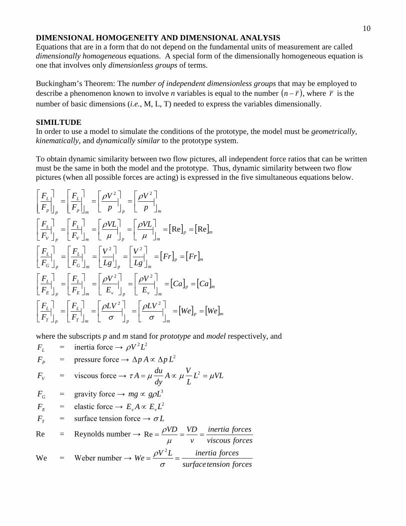
10 DIMENSIONAL HOMOGENEITY AND DIMENSIONAL ANALYSIS Equations that are in a form that do not depend on the fundamental units of measurement are called dimensionally homogeneous equations. A special form of the dimensionally homogeneous equation is one that involves only dimensionless groups of terms. Buckingham’s Theorem: The number of independent dimensionless groups that may be employed to describe a phenomenon known to involve n variables is equal to the number ( )rn − , where r is the number of basic dimensions (i.e., M, L, T) needed to express the variables dimensionally. SIMILTUDE In order to use a model to simulate the conditions of the prototype, the model must be geometrically, kinematically, and dynamically similar to the prototype system. To obtain dynamic similarity between two flow pictures, all independent force ratios that can be written must be the same in both the model and the prototype. Thus, dynamic similarity between two flow pictures (when all possible forces are acting) is expressed in the five simultaneous equations below.

[ ] [ ]

[ ] [ ]

[ ] [ ]

[ ] [ ]mpmpmT

L

pT

L

mpmvpvmE

L

pE

L

mpmpmG

L

pG

L

mpmpmV

L

pV

L

mpmp

L

pp

L

WeWeLVLVFF

FF

CaCaEV

EV

FF

FF

FrFrLgV

LgV

FF

FF

VLVLFF

FF

pV

pV

FF

FF

==

=

=

=

==

=

=

=

==

=

=

=

==

=

=

=

=

=

=

σρ

σρ

ρρ

µρ

µρ

ρρ

22

22

22

22

ReRe

where the subscripts p and m stand for prototype and model respectively, and

LF = inertia force → 22 LVρ

PF = pressure force → 2LpAp ∆∝∆

VF = viscous force → VLLLVA

dyduA µµµτ =∝= 2

GF = gravity force → 3Lgmg ρ∝

EF = elastic force → 2LEAE vv ∝

TF = surface tension force → Lσ

Re = Reynolds number → forcesviscousforcesinertia

vVDVD

===µ

ρRe

We = Weber number → forcestensionsurface

forcesinertiaLVWe ==σ

ρ 2

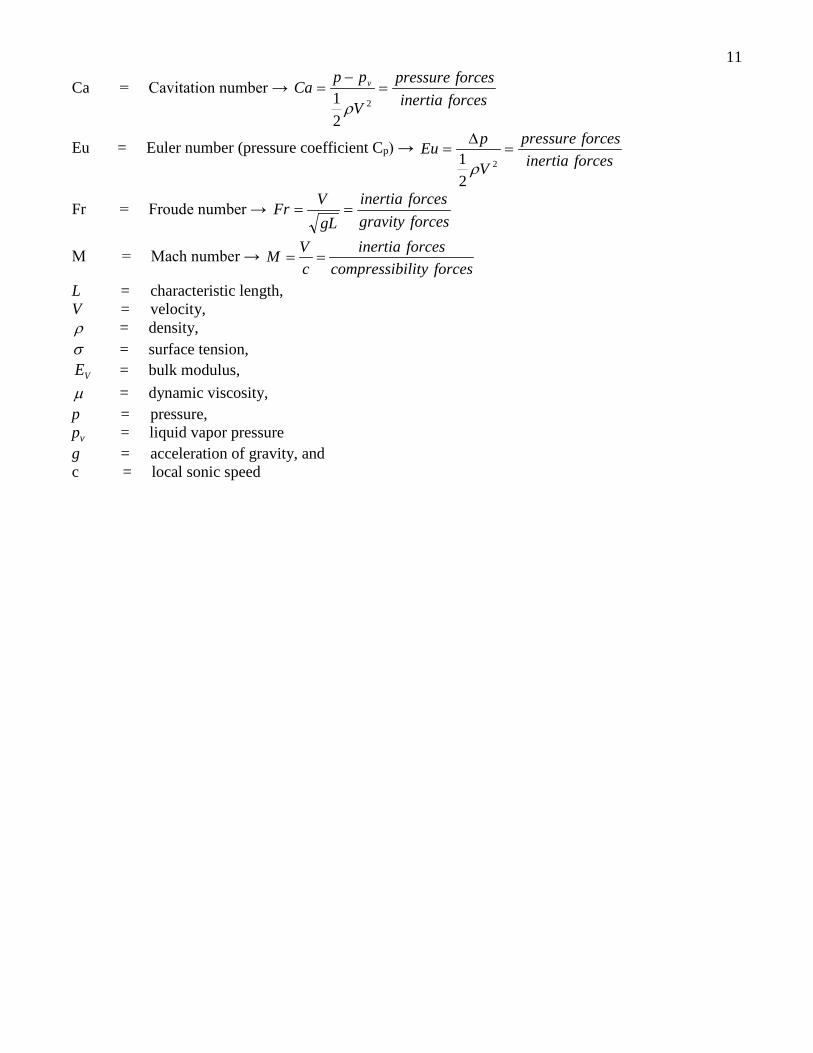
11

Ca = Cavitation number → forcesinertiaforcespressure

V

ppCa v =

−=

2

21 ρ

Eu = Euler number (pressure coefficient Cp) → forcesinertiaforcespressure

V

pEu =∆

=2

21 ρ

Fr = Froude number → forcesgravityforcesinertia

gLVFr ==

M = Mach number → forcesilitycompressib

forcesinertiacVM ==

L = characteristic length, V = velocity, ρ = density, σ = surface tension,

VE = bulk modulus, µ = dynamic viscosity, p = pressure, pv = liquid vapor pressure g = acceleration of gravity, and c = local sonic speed