Relativistic Brownian Motion

Relativistic Brownian Motion

Yue Wang, Prof. Rajeev

April 26, 2021

Abstract

The displacements of a particle from classical Brownian motion forma Gaussian distribution. However, the distribution of variables drawnfrom a distribution with infinite variance as opposed to a finite variancein classical Brownian motion is not Gaussian. We show that the sum of alarge number of lognormal variables tends to an α-stable Levy subordina-tor when 0 < α < 1. This distribution is surprisingly common in real-lifestochastic systems such as stock market and relativistic Brownian motion.

1 Introduction

1.1 Background

In classical Brownian Motion, defined below, the speed of particles has beenassumed to be infinite and the displacement of each step has been treated asindependent.[1]

Definition 1.1. (classical Brownian Motion) A real-valued stochastic pro-cess B(t) : t ≥ 0 is called a classical Brownian motion with start in x ∈ R ifthe following holds:

1. B(0) = x,

2. the process has independent increments, i.e. for all times 0 ≤ t1 ≤ t2 ≤... ≤ tn the increments B(tn) − B(tn−1), B(tn−1) − B(tn−2), ..., B(t2) −B(t1) are independent random variables,

3. for all t ≥ 0 and h > 0, the increments B(t + h) − B(t) are normallydistributed with expectation zero and variance h,

4. almost surely, the function t→ B(t) is continuous.

We say that B(t) : t ≥ 0 is a classical Brownian motion.

1

1 INTRODUCTION 2

1.2 Model Construction

The velocity of particles in classical Brownian motion are assumed to be infinite.However, in reality, the speed of particles is bounded above by the speed of lightc. We are interested in studying the motion of the particles moving at nearlythe speed of light. Therefore, this study requires relativity.

Velocity is the derivative of position with respect to time. In relativity, amore natural variable is rapidity θ, which is related to the derivative of positionX1 and time X0 with respect to proper time τ (time measured by a clockattached to the particle). In units with c = 1,

dX0

dτ= cosh θ,

dX1

dτ= sinh θ.

We can see that the relation of velocity to rapidity is

v =dX1

dX0= tanh θ.

Although θ is not bounded, v is bounded by the speed of light.It is more convenient to introduce null co-ordinates

X0 ±X1 = X±

so thatdX+

dτ= eθ,

dX−

dτ= e−θ.

Thus, we can now propose a model of relativistic Brownian motion in onespatial dimension.

A particle moves along a straight line until it collides with another particle.In each collision, the rapidity of a particle is changed by the addition of a randomvariable. The effect of a large number of such collisions is to make rapidity intoa Gaussian random variable (Central Limit Theorem). The null coordinates areincremented by the exponential of rapidity at each step:

X+k = X+

k−1 + eθk∆τ, X−k = X−k−1 + e−θk∆τ

where ∆τ is a small interval of proper time in between two collisions. Also, θkare independent identically distributed (i.i.d) Gaussian random variables.

Thus we have

X+n = ∆τ

n∑k=1

eθk

and similarly for X−n . The mathematical question we solve is how to take thelimit n→∞ and ∆τ → 0 such that Xn tends to a random process.

We should expect that this limit is an infinitely divisible distribution, becausethe sum can be subdivided into independent terms. Because the terms in thesum are positive, we should expect also that this will be a “subordinate process”

1 INTRODUCTION 3

in the sense defined below. A tricky question is how the mean and variance ofthe Gaussian random variables θk must behave as n→∞.

If θ is Gaussian, x = eθ is log-normal. It is useful to write its probabilitydensity function in the following form:

Proposition 1.2. The probability measure of a log-normal variable can be writ-ten as

µ(dx) =1

Z

e−log2 x

2σ2

xα+1dx

whereE (log x) = −ασ2, Var (log x) = σ2

and

Z =√

2πσeα2σ2

2 .

Proof. Make the change of variables θ = log x

µ(dx) =1

Z

e−θ2

2σ2

e(α+1)θeθdθ

=1

Ze−

12σ2

θ2−αθdθ

=eα2σ2

2

Ze−

12σ2

[θ+ασ2]2

dθ

=1√2πσ

e−1

2σ2[θ+ασ2]

2

dθ.

This is the probability density of a normal variable with mean −ασ2 andvariance σ2.

We will hold α fixed as n → ∞. The question then is how the varianceσ2 must depend on n in order that the sum of n identical log-normal variablestends to a sensible limit as n→∞. We will show below that we need

σ2n ∼

log[α2n2

2π

]α2

.

Since the variance tends to infinity, the central limit theorem does not applyand the limiting distribution for Xn is not a Gaussian, unlike for Brownianmotion. Instead, it will be an α-stable subordinator Levy distribution. This isour main result.

In the next section, we will review some useful results from the theory ofstochastic processes.

2 THEORETICAL DERIVATION 4

1.3 Impact

A few studies were published on related problems. The distribution of the sumof log-normal variables was studied as early as in 1960.[2] A comparison of fourmethods to approach the sum of log-normal variables was published in 1995.[3]In 2003, a paper focusing on using moment-matching approximation to studythe distribution of the sum of log-normal variables was published.[4]

The distribution of log-normal variables with additional parameters fromfinancial models was studied in 1998 and the distribution of independent but notnecessarily identically distributed log-normal variables was studied in 2005.[5][6]In 2008, a paper was published on the asymptotics of the sum of log-normalvariables.[7]

In this paper, we will show that the sum of log-normal variables tends toan infinitely divisible α-stable Levy subordinator when the number of terms ofin the sum goes to infinity. α is the ratio of the mean to the variance of thenormal distribution and we will focus on the case when 0 < α < 1. However,this approach is very slow and the number of steps is expected to be much largerthan 500.

The resulting distribution of relativistic Brownian motion is quite commonin real-life stochastic systems including stock market. In the future, this workcan be generalized into financial field.

We will first present our theoretical derivation, with special emphasize onthe major approximations and normalizations. In the following section, wewill present a numerical verification of the proposed distribution. Finally, ourmethods will be demonstrated using a simulation program.

2 Theoretical Derivation

First, we state the definition of a Levy process.[8]

Definition 2.1. (Levy Process) Let X = (X(t), t ≥ 0) be a stochastic pro-cess defined on a probability space (Ω,F , P ). We say that it has independentincrements if for each n ∈ N and each 0 ≤ t1 < t2 < ... < tn+1 < ∞ therandom variables (X(tj+1)−X(tj), 1 ≤ j ≤ n) are independent and that it has

stationary increments if each X(tj+1)−X(tj)d= X(tj+1 − tj)−X(0).

We say that X is a Levy process if:

1. X(0) = 0 (almost surely);

2. X has independent and stationary increments;

3. X is stochastically continuous, i.e. for all a > 0 and for all s ≥ 0

limt→s+

P (|X(t)−X(s)| > a) = 0.

The third property of Levy process implies that Levy processes are notnecessarily continuous. In fact, classical Brownian motion is the only Levy


process that is continuous. Our model for relativistic Brownian motion is notcontinuous. However, it is infinitely divisible.[8]

Definition 2.2. (Infinitely Divisible) Let X be a random variable takingvalues in Rd with law µX . We say that X is infinitely divisible if, for all n ∈N, there exist independent and identically distributed (i.i.d.) random variables

Y(n)1 , ..., Y

(n)n such that

Xd= Y

(n)1 + ...+ Y (n)

n .

2.1 Problem Reduction

The following theorem guarantees the infinite divisibility of relativistic Brownianmotion once the motion is shown to be a Levy process.[8]

Theorem 2.3. If X is a Levy process, then X(t) is infinitely divisible for eacht ≥ 0.

Proof. For each n ∈ N, define

Y(n)k (t) = X

(ktn

)−X

( (k − 1)t

n

).

Y(n)k (t) are i.i.d. for each 1 ≤ k ≤ n by the second property from the

definition for Levy process.Therefore, for such n, we have

X(t) = Y(n)1 (t) + ...+ Y (n)

n (t).

By definition, X(t) is infinitely divisible.

Therefore, we have reduced the problem to showing the sum of log-normalvariables tends to an α-stable subordinator Levy distribution.

We now introduce five definitions.[8][9]

Definition 2.4. (Stable Random Variables) We consider the general cen-tral limit problem in dimension d = 1, so let (Yn, n ∈ N) be a sequence ofreal-valued i.i.d. random variables and construct the sequence (Sn, n ∈ N) ofrescaled partial sums

Sn =Y1 + Y2 + ...+ Yn − bn

σn,

where (bn, n ∈ N) is an arbitrary sequence of real numbers and (σn, n ∈ N)an arbitrary sequence of positive numbers. We are interested in the case wherethere exists a random variable X for which

limn→∞

P (Sn ≤ x) = P (X ≤ x) (1)

for all x ∈ R, i.e. (Sn, n ∈ N) converges in distribution to X.A random variable is said to be stable if it arises as a limit as in Equation

1.


Definition 2.5. (Stable Levy Processes) A stable Levy process is a Levyprocess X in which each X(t) is a stable random variable

Definition 2.6. (α-stable Levy Processes) Let Xt : t ≥ 0 be a Levyprocess on Rd. It is called α-stable if, for any a > 0, there is α such that

Xat : t ≥ 0 d= a 1

αXt : t ≥ 0.

Definition 2.7. (Subordinator) A subordinator is a one-dimensional Levyprocess that is non-decreasing (almost surely).

More specifically, α-stable subordinators are defined as the following.

Definition 2.8. (α-stable Subordinators) An α-stable subordinator X isa Levy process with E

(e−uX

)= e−u

α

for 0 < α < 1, u ≥ 0.

Using the identity (the proof of which we will recall in section 2.7),

uα =α

Γ(1− α)

∫ ∞0

(1− e−ux

) dx

x1+α.

It follows that the problem has been reduced to showing

logE(e−uX

)=

∫ ∞0

(1− e−ux

) dx

x1+α. (2)

2.2 Definition of Variables

We are interested in the expected value for the exponential of displacement. Inthe following derivation, we will use the following notation:

n: the number of steps;x: step, the log-normal variable;Xn: displacement after n steps;X = limn→∞Xn;s: time window;σ2: the variance of rapidity;−ασ2: the mean of rapidity.µn(dx): the probability measure.Since every step is independent

E(e−sXn) = [

∫ ∞0

e−sxµn(dx)]n.

∫∞0e−sxµn(dx) is the expected value for the exponential of each step x. The

summation of the expected value of each step becomes multiplication whentaking the exponential.

If we choose∫∞0nµn(dx) = 1,

E(e−sXn) = [1 +1

n

∫ ∞0

(e−sx − 1)nµn(dx)]n


E(e−sXn) = exp[n log(1 +1

n

∫ ∞0

(e−sx − 1)nµn(dx))]. (3)

This equation allows us to further simplify the expression for E(e−sXn) usingapproximations, which will be explained in the following sections.

2.3 Large Number Approximation

Assuming n is large so that 1n is small.

Consider the Taylor expansion around x = 0,

log(1 + x) = x− x2

2+ ...

When x is sufficiently small, the first two or one terms is a good approxima-tion for log(1 + x). We now apply this approximation to Equation 3.

The Taylor expansion for Equation 3 is

exp[

∫ ∞0

(e−sx − 1)nµn(dx)− 1

2n[

∫ ∞0

(e−sx − 1)nµn(dx)]2] + ...

Since 1n is sufficiently small, only keeping first two terms in its Taylor ex-

pansion gives a good approximation for E(e−sXn), as shown in Equation 4.

E(e−sXn) = exp[

∫ ∞0

(e−sx − 1)nµn(dx)− 1

2n[

∫ ∞0

(e−sx − 1)nµn(dx)]2]. (4)

Moreover, if we only keep the first term,

E(e−sXn) = exp[

∫ ∞0

(e−sx − 1)nµn(dx)]. (5)

2.4 Normalization

Before deriving Equation 5 further, it is critical to study its properties in limitcases. If µn does not depend on n, the integral in Equation 5 goes to infinityas n goes to infinity, which is not physical. To eliminate the n dependence inEquation 5, we choose µn such that nµn does not depend on n. Physically, thechange of n means a change of the number of steps in a fixed time window.By dividing the given time window into finer bins, we do not expect to receivelarger and larger total displacement happening within the time window.

Recall the log-normal probability density function. This measure is usedsince the variable x follows a log-normal distribution.

µn(dx) =1

Zσ,α

exp(− log2 x2σ2 )

xα+1dx

where

Zσ,α =√

2πσeα2σ2

2


We choose σn so thatZσn,α = n.

Then

nµn(dx) =n

Zσn,α

exp(− log2 x2σ2n

)

xα+1dx =

exp(− log2 x2σ2n

)

xα+1dx (6)

which is independent of n. This normalizes E(e−sXn).By solving Zσn,α = n, we have

σ2n =

W (α2n2

2π )

α2. (7)

where W (z) is the Lambert function, defined as the principal branch solutionof z = W (z)eW (z).

2.5 Very Large Number Approximation

We simplify Equation 7 by assuming n is even larger so that 1logn is small.

Expanding the Lambert function introduced above,

W (z) = log z − log log z +O(1)

Since 1logn is small, we can approximate W (z) only keep the first term in the ex-

pansion. Substituting W (α2n2

2π ) by the first term from its expansion in Equation7,

σ2n =

log(α2n2

2π )

α2.

Applying this result and the expression for nµn in Equation 6 to Equation 5,we have

E(e−sX) = exp[

∫ ∞0

(e−sx − 1)exp(− log2 x

2σ2n

)

xα+1dx]. (8)

2.6 Another Large Number Approximation

Equation 8 can be further simplified assuming n → ∞, then log2 x2σ2n

is small.

Therefore, we can approximate exp(− log2 x2σ2n

) by 1. With this approximation,

Equation 8 becomes

E(e−sX) = exp[

∫ ∞0

(e−sx − 1)1

xα+1dx]. (9)

Thus,

logE(e−sX) =

∫ ∞0

(e−sx − 1)1

xα+1dx.

This agrees with Equation 2, so the sum of log-normal variables in relativisticBrownian motion is an infinitely divisible α-stable Levy subordinator as long asthe integral

∫∞0

[1 − e−sx] dxxα+1 converges. Notice that the integral on the right

hand side converges when 0 < α < 1.


2.7 Alternative Large Number Approximation: First Or-der

Instead of applying the approximation in the previous section, which is exp(− log2 x2σ2n

)→1, consider the following Taylor expansion.

∫ ∞0

(e−sx−1)exp(− log2 x

2σ2n

)

xα+1dx =

∫ ∞0

(e−sx−1)1

xα+1dx− 1

2σ2n

∫ ∞0

log2 x

xα+1[e−sx−1]dx+...

Furthermore, following the derivation by Applebaum, we can prove the identitymentioned in section 2.1.[8] For 0 < α < 1,∫ ∞

0

(e−sx − 1)1

xα+1dx =

∫ ∞0

(

∫ x

0

se−sydy)dx

xα+1

=

∫ ∞0

(

∫ ∞y

dx

xα+1)se−sydy

= − sα

∫ ∞0

e−syy−αdy

= −sα

α

∫ ∞0

e−xx−αdx

= −sα

αΓ(1− α)

= −sα

α(−α)Γ(−α)

= sαΓ(−α)

Therefore,logE(e−sX) = sαΓ(−α).

Moreover, since

−sα

αΓ(1− α) = sαΓ(−α),

sαΓ(−α) =

∫ ∞0

[e−sx − 1]dx

xα+1.

Hence,

∫ ∞0

(e−sx − 1)exp(− log2 x

2σ2n

)

xα+1dx→ Γ(−α)sα − 1

2σ2n

∫ ∞0

log2 x

xα+1[e−sx − 1]dx+ ...

If we only keep the first order in this expansion

E(e−sX) = exp[Γ(−α)sα]. (10)

3 NUMERICAL VERIFICATION 10

In other words,

logE(e−sX) =

∫ ∞0

(e−sx − 1)1

xα+1dx.

This matches Equation 2. Hence, we conclude that the sum of log-normalvariables in relativistic Brownian motion is an infinitely divisible α-stable Levysubordinator as long as the integral

∫∞0

[1− e−sx] dxxα+1 converges.

When α = 12 , there is an analytic expression for the Γ function. Then

Equation 10 becomesE(e−sX) = exp(−2π

12 s

12 ). (11)

Thus, we have shown that the sum of log-normal variables in relativisticBrownian motion is an infinitely divisible α-stable Levy subordinator for 0 <α < 1.

2.8 Alternative Large Number Approximation: SecondOrder

To include the second order term in the expansion, Recall for 0 < α < 1,

sαΓ(−α) =

∫ ∞0

[e−sx − 1]dx

xα+1.

Also

− ∂

∂α(

1

xα+1) =

log x

xα+1.

Furthermore,∂2

∂α2(

1

xα+1) =

log2 x

xα+1.

Then∂2

∂α2(sαΓ(−α)) =

∫ ∞0

log2 x[e−sx − 1]dx

xα+1.

So

E(e−sXn) = exp[Γ(−α)sα − 1

2σ2n

∂2

∂α2(sαΓ(−α))].

This is an infinitely divisible α-stable Levy subordinator with a correctionterm.

3 Numerical Verification

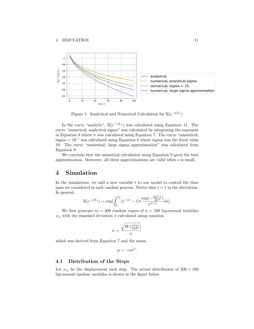
We study the case when α = 12 using numerical verification. E(e−sXn) has been

calculated analytically and numerically when n = 104.

4 SIMULATION 11

Figure 1: Analytical and Numerical Calculation for E(e−sXn)

In the curve “analytic”, E(e−sXn) was calculated using Equation 11. Thecurve “numerical; analytical sigma” was calculated by integrating the exponentin Equation 8 where σ was calculated using Equation 7. The curve “numerical;sigma = 10.” was calculated using Equation 8 where sigma was the fixed value10. The curve “numerical; large sigma approximation” was calculated fromEquation 9.

We conclude that the numerical calculation using Equation 9 gives the bestapproximation. Moreover, all three approximations are valid when s is small.

4 Simulation

In the simulations, we add a new variable t to our model to control the timespan we considered in each random process. Notice that t = 1 in the derivation.In general,

E(e−sXn) = exp[

∫ ∞0

(e−sx − 1)texp(− log2 x

2σ2 )

xα+1dx].

We first generate m = 200 random copies of n = 100 log-normal variablesxij with the standard deviation σ calculated using equation

σ =

√W (α

2n2

2πt2 )

α

which was derived from Equation 7 and the mean

µ = −ασ2.

4.1 Distribution of the Steps

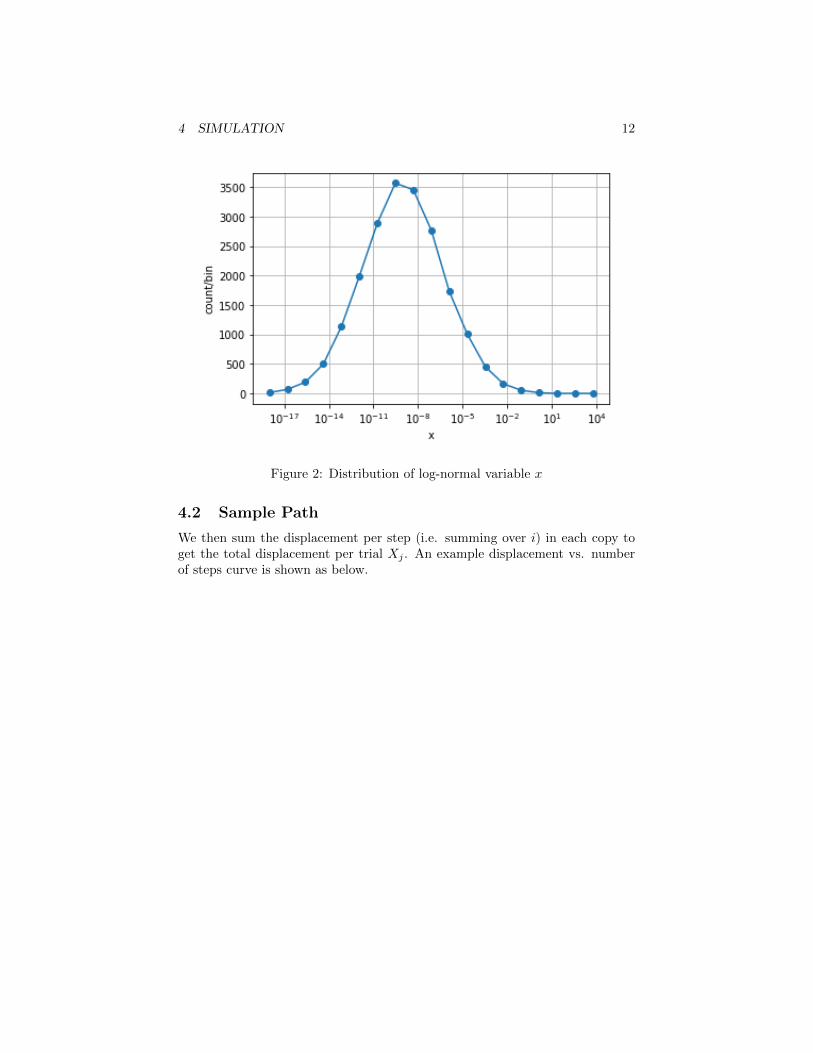
Let xij be the displacement each step. The actual distribution of 200 × 100log-normal random variables is shown in the figure below.

4 SIMULATION 12

Figure 2: Distribution of log-normal variable x

4.2 Sample Path

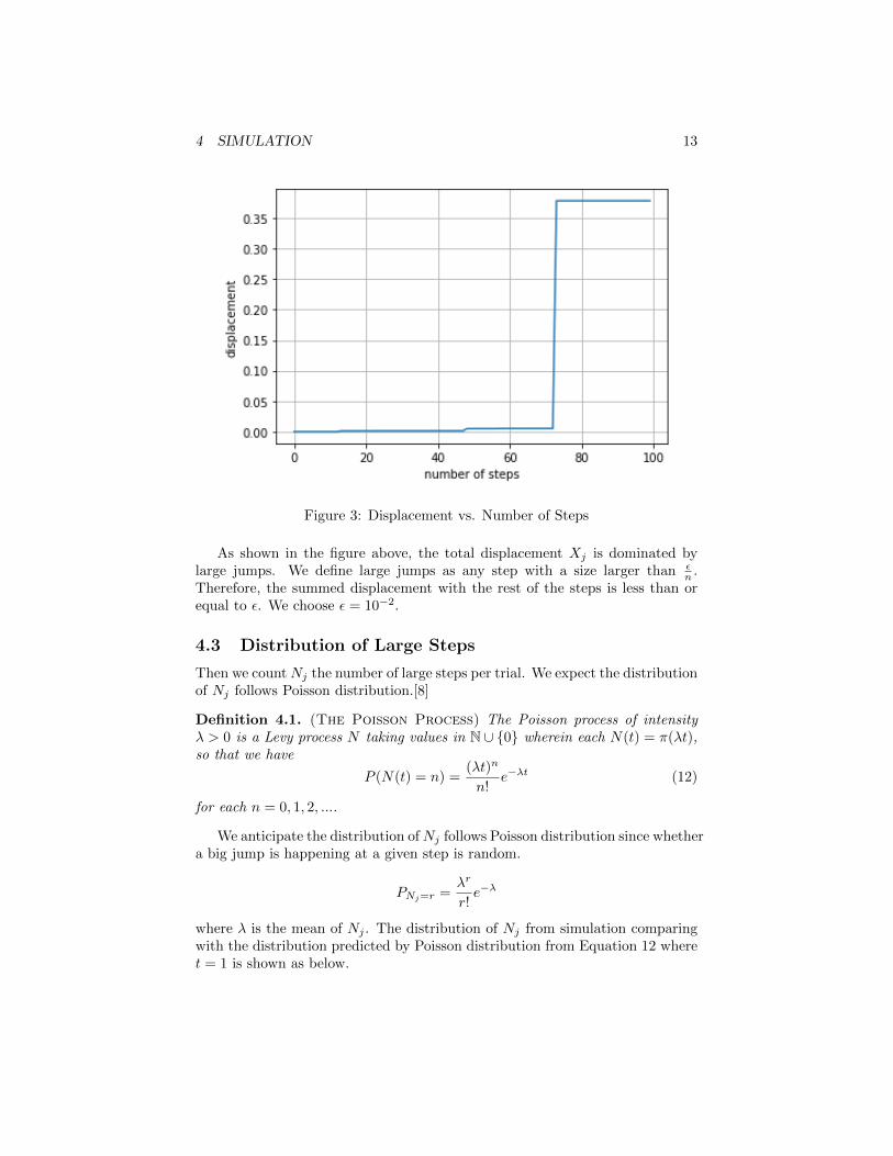
We then sum the displacement per step (i.e. summing over i) in each copy toget the total displacement per trial Xj . An example displacement vs. numberof steps curve is shown as below.

4 SIMULATION 13

Figure 3: Displacement vs. Number of Steps

As shown in the figure above, the total displacement Xj is dominated bylarge jumps. We define large jumps as any step with a size larger than ε

n .Therefore, the summed displacement with the rest of the steps is less than orequal to ε. We choose ε = 10−2.

4.3 Distribution of Large Steps

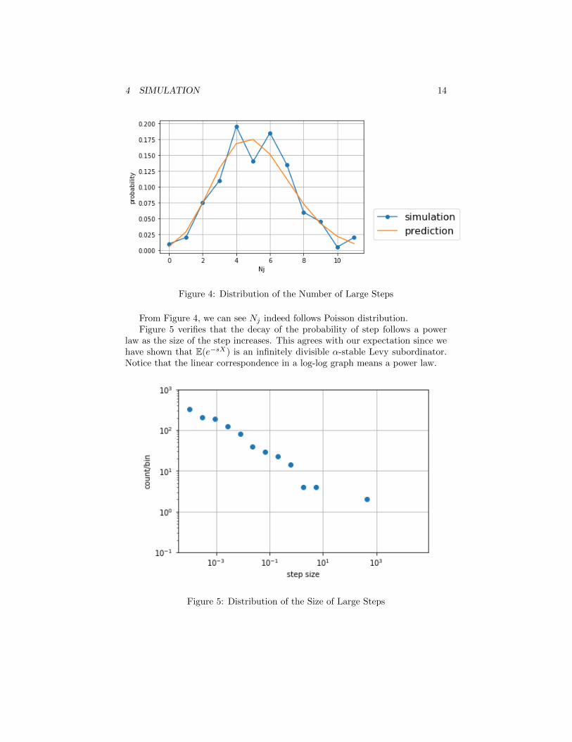
Then we countNj the number of large steps per trial. We expect the distributionof Nj follows Poisson distribution.[8]

Definition 4.1. (The Poisson Process) The Poisson process of intensityλ > 0 is a Levy process N taking values in N ∪ 0 wherein each N(t) = π(λt),so that we have

P (N(t) = n) =(λt)n

n!e−λt (12)

for each n = 0, 1, 2, ....

We anticipate the distribution ofNj follows Poisson distribution since whethera big jump is happening at a given step is random.

PNj=r =λr

r!e−λ

where λ is the mean of Nj . The distribution of Nj from simulation comparingwith the distribution predicted by Poisson distribution from Equation 12 wheret = 1 is shown as below.

4 SIMULATION 14

Figure 4: Distribution of the Number of Large Steps

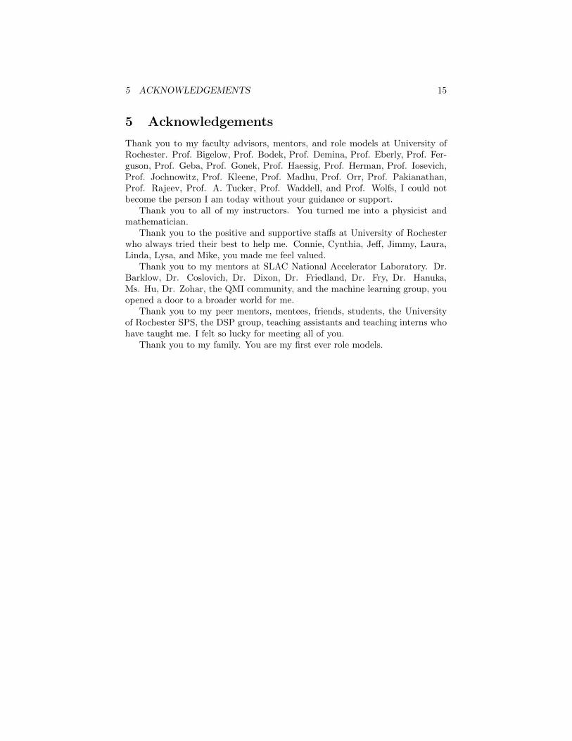
From Figure 4, we can see Nj indeed follows Poisson distribution.Figure 5 verifies that the decay of the probability of step follows a power

law as the size of the step increases. This agrees with our expectation since wehave shown that E(e−sX) is an infinitely divisible α-stable Levy subordinator.Notice that the linear correspondence in a log-log graph means a power law.

Figure 5: Distribution of the Size of Large Steps

5 ACKNOWLEDGEMENTS 15

5 Acknowledgements

Thank you to my faculty advisors, mentors, and role models at University ofRochester. Prof. Bigelow, Prof. Bodek, Prof. Demina, Prof. Eberly, Prof. Fer-guson, Prof. Geba, Prof. Gonek, Prof. Haessig, Prof. Herman, Prof. Iosevich,Prof. Jochnowitz, Prof. Kleene, Prof. Madhu, Prof. Orr, Prof. Pakianathan,Prof. Rajeev, Prof. A. Tucker, Prof. Waddell, and Prof. Wolfs, I could notbecome the person I am today without your guidance or support.

Thank you to all of my instructors. You turned me into a physicist andmathematician.

Thank you to the positive and supportive staffs at University of Rochesterwho always tried their best to help me. Connie, Cynthia, Jeff, Jimmy, Laura,Linda, Lysa, and Mike, you made me feel valued.

Thank you to my mentors at SLAC National Accelerator Laboratory. Dr.Barklow, Dr. Coslovich, Dr. Dixon, Dr. Friedland, Dr. Fry, Dr. Hanuka,Ms. Hu, Dr. Zohar, the QMI community, and the machine learning group, youopened a door to a broader world for me.

Thank you to my peer mentors, mentees, friends, students, the Universityof Rochester SPS, the DSP group, teaching assistants and teaching interns whohave taught me. I felt so lucky for meeting all of you.

Thank you to my family. You are my first ever role models.

REFERENCES 16

References

[1] Peter Morters and Yuval Peres. Brownian Motion. Cambridge UniversityPress, 2010.

[2] L. Fenton. The sum of log-normal probability distributions in scatter trans-mission systems. IRE Transactions on Communications Systems, 8(1):57–67, 1960.

[3] N. C. Beaulieu, A. A. Abu-Dayya, and P. J. McLane. Estimating the distri-bution of a sum of independent lognormal random variables. IEEE Trans-actions on Communications, 43(12):2869, 1995.

[4] S. M. Haas and J. H. Shapiro. Capacity of wireless optical communications.IEEE Journal on Selected Areas in Communications, 21(8):1346–1357, 2003.

[5] Moshe Arye Milevsky and Steven E. Posner. Asian options, the sum of log-normals, and the reciprocal gamma distribution. The Journal of Financialand Quantitative Analysis, 33(3):409–422, 1998.

[6] Jingxian Wu, N. B. Mehta, and Jin Zhang. Flexible lognormal sum approx-imation method. In GLOBECOM ’05. IEEE Global TelecommunicationsConference, 2005., volume 6, pages 3413–3417, Nov 2005.

[7] Søren Asmussen and Leonardo Rojas-Nandayapa. Asymptotics of sums oflognormal random variables with gaussian copula. Statistics ProbabilityLetters, 78(16):2709 – 2714, 2008.

[8] David Applebaum. Levy Processes and Stochastic Calculus, volume 93. Cam-bridge University Press, Cambridge, 2004.

[9] Ken-iti Sato. Levy processes and infinitely divisible distributions. Cambridgestudies in advanced mathematics ; 68. Cambridge University Press, Cam-bridge, United Kingdom, rev. edition, corrected paperback edition. edition,2013.

17

AppendicesNumerical Verification Program

#!/usr/bin/env python

# coding: utf-8

# In[ ]:

#Authors: Yue Wang, Prof. Rajeev

# In[2]:

#packages

import math

import numpy as np

import matplotlib.pyplot as plt

import scipy as sp

from scipy.optimize import curve_fit

# In[3]:

#alpha in the derivation and in alpha-stable Poisson process

alpha = 0.5

# In[4]:

#integrate the integral in the alpha-stable subordinator equation

numerically

#fixed sigma = 10.

def zexp(m,s,alpha):

#integration method

sigma =

10.#np.sqrt(sp.special.lambertw(alpha**2*m**2/(2*math.pi)))/alpha

#print(sigma)

binNum = 10**4

binSize = 10**(-3)

integral = 0.0

for i in range(1,binNum):#iterate through the waves collected

x = i*binSize

integral = integral +

(np.exp(-s*x)-1)*(np.exp(-(np.log(x))**2/(2*sigma**2))/(x**(alpha+1)))*binSize

18

return integral

# In[5]:


numerically

#sigma without approximation

#analytic sigma

def zexpAnalytic(m,s,alpha):

#integration method

sigma = np.sqrt(sp.special.lambertw(alpha**2*m**2/(2*math.pi)))/alpha

#print(sigma)

binNum = 10**4

binSize = 10**(-3)

integral = 0.0


x = i*binSize

integral = integral +

(np.exp(-s*x)-1)*(np.exp(-(np.log(x))**2/(2*sigma**2))/(x**(alpha+1)))*binSize

return integral

# In[8]:


numerically

#large sigma approximation

def z(m,s,alpha):

#integration method

binNum = 10**4

binSize = 10**(-3)

integral = 0.0


x = i*binSize

integral = integral + (np.exp(-s*x)-1)/(x**(1+alpha))*binSize

return integral

# In[15]:

#Integrate Z with different sigma approximations

binNumSplot = 10**2

binSize = 1

plotListZ = []

plotListS = []

19

plotListA = []

plotListZExp = [] #fixed sigma

plotListZExpA = [] #analytic

plotListZExp1 = [] #1st approximation

plotListZExp2 = [] #2nd approximation

for i in range (3,4):

m = 10**i

sList = []#list of s values

zList = []

aList = []

zExpList = []

zExpAList = []

zExp1List = []

zExp2List = []

for j in range(1,binNumSplot):

sList.append(j*binSize)

zList.append(z(1,j*binSize,alpha))

aList.append(-2*np.pi**(1/2)*(j*binSize)**(1/2))

zExpList.append(zexp(m,j*binSize,alpha))

zExpAList.append(zexpAnalytic(m,j*binSize,alpha))

zExp1List.append(zexp1(m,j*binSize,alpha))

zExp2List.append(zexp2(m,j*binSize,alpha))

plotListS.append(sList)

plotListZ.append(zList)

plotListA.append(aList)

plotListZExp.append(zExpList)

plotListZExpA.append(zExpAList)

plotListZExp1.append(zExp1List)

plotListZExp2.append(zExp2List)

# In[19]:

#Plot Z integrated using different sigma approximations

for i in range(1):

plt.plot(plotListS[i],plotListA[i],label = ’analytical’)

plt.plot(plotListS[i],plotListZExpA[i],label = ’numerical;

analytical sigma’)

plt.plot(plotListS[i],plotListZExp[i],label = ’numerical; sigma =

10.’)

plt.plot(plotListS[i],plotListZ[i],label = ’numerical; large sigma

approximation’)

plt.xlabel(’s(a.u.)’)

plt.ylabel(’z(a.u.)’)

plt.legend(loc=(1.05,0.1),fontsize=16.0)

plt.grid()

#plt.show()

plt.savefig(’numericalZ.png’,bbox_inches=’tight’)

20

Simulation Program

#!/usr/bin/env python

# coding: utf-8

# In[ ]:

#Authors: Yue Wang, Prof. Rajeev

# In[43]:

#packages

import math

import numpy as np

import matplotlib.pyplot as plt

import scipy as sp

from scipy.optimize import curve_fit

import numpy.ma as ma

# In[44]:

#epsilon in the derivation: used to define large steps

epsilon = 10**(-2)

#t: time range

t = 0.05

# In[45]:

#alpha in the derivation and in alpha-stable Poisson process

alpha = 1/2

n=100 #number of steps

m = 200 #number of copies

sigma =

np.sqrt(sp.special.lambertw((alpha**2)*(n**2)/(2*math.pi*(t**2))))/alpha

mu = -alpha*sigma**2 #from the mathematica program

# In[47]:

#generate steps

xList = [] #X_ij

distList = [] #the list of summed x for each copy; X_j

21

for i in range(0,m):

theta = np.random.normal(0., 1.0, n)

x = np.exp(sigma*theta+mu)

xList.append(x)

distList.append(sum(x))

# In[48]:

#boolean list indicating if the each step in xList is large

booleanList = np.array(xList)[:][:]>epsilon/n

# In[49]:

NList = [] #N_j

for j in range(0,m):

NList.append(sum(booleanList[j]))

# In[56]:

#histogram for number of large steps

Nhist,Nbin= np.histogram(NList,bins =12)

plt.plot(Nbin[:-1],Nhist,’o-’)

plt.xlabel(’Nj’)

plt.ylabel(’count/bin’)

#plt.yscale("log")

#plt.xlim(0,10)

#plt.ylim(top=1000)

#plt.ylim(top=2200)

plt.grid()

# In[58]:

#define the Poisson distribution

#suppose the Poisson process is called N

#lambda_poisson is a float, which is the mean of of N

#r_possion is a float. It matches with the r in the main text

def poisson(lambda_poisson, r_possion):

return

((lambda_poisson**r_possion)/(math.factorial(r_possion)))*np.exp(-lambda_poisson)

22

# In[59]:

#plot the expectated curve using values from Nbin as r values

#Nbin contains the x axis values in the histogram for number of large

steps

poissonPlot = []

for Nj in Nbin[:-1]:

poissonPlot.append(poisson(np.mean(NList),math.floor(Nj)))

# In[76]:

#histogram for number of large steps with expected poisson distribution

plt.plot(Nbin[:-1],Nhist/sum(Nhist),’o-’,label = ’simulation’)

plt.plot(Nbin[:-1],poissonPlot,label = ’prediction’)

plt.xlabel(’Nj’)

plt.ylabel(’probability’)

plt.legend(loc=(1.05,0.1),fontsize=16.0)

#plt.yscale("log")

#plt.xlim(0,10)

#plt.ylim(top=50)

#plt.ylim(top=2200)

plt.grid()

plt.savefig(’largestep.png’,bbox_inches=’tight’)

# In[75]:

#histogram for step sizes

#Lognormal

disthist, distbin = np.histogram(np.array(xList).flatten(),bins

=np.logspace(-18,5,20))

plt.plot(distbin[:-1],disthist,’o-’)

plt.xlabel(’x’)


plt.xscale("log")

#plt.xlim(0,10)

#plt.ylim(top=1000)

#plt.ylim(top=2200)

plt.grid()

plt.savefig(’xhistogram.png’,bbox_inches=’tight’)

# In[62]:

23

#boolean matrix transpose

booleanListI = np.invert(booleanList)

# In[63]:

#select large steps in xList

mx = ma.masked_array(np.array(xList), mask=np.array(booleanListI))

print(mx)

# In[64]:

#select large steps

compressedMx = []

compressedMxFlattened = []

for j in range(len(mx)):

compressedX = mx[j].compressed()

buffer = []

for i in range(len(compressedX)):

buffer.append(float(compressedX[i]))

compressedMxFlattened.append(float(compressedX[i]))

compressedMx.append(buffer)

# In[79]:

#histogram for the sizes of large steps

#log-log normal

largehist, largebin = np.histogram(compressedMxFlattened,bins

=np.logspace(-4,5,20))

plt.plot(largebin[:-1],largehist,’o’)

plt.xlabel(’step size’)


plt.xscale("log")

plt.yscale("log")

#plt.xlim(0,10)

#plt.ylim(top=1000)

plt.ylim(10**(-1),10**3)

plt.grid()

plt.savefig(’largestepsize.png’,bbox_inches=’tight’)

# In[66]:

24

#plot a sample path

samplePath = []

for i in range(0,n):

samplePath.append(sum(xList[0][:i]))

# In[67]:

#plot one path

plt.plot(samplePath)

plt.xlabel(’number of steps’)

plt.ylabel(’displacement’)

#plt.yscale("log")

#plt.xlim(0,10)

#plt.ylim(top=50)

#plt.ylim(top=2200)

plt.grid()

plt.savefig(’examplePath.png’,bbox_inches=’tight’)

Relativistic Brownian Motion

Documents

Transcript of Relativistic Brownian Motion