Relating discrete and continuum 2d quantum gravity
151
RU Nijmegen, Apr. 14, 2014 Relating discrete and continuum 2d quantum gravity Timothy Budd Niels Bohr Institute, Copenhagen. [email protected], http://www.nbi.dk/ ~ budd/
-
Upload
timothy-budd -
Category
Science
-
view
23 -
download
0
Transcript of Relating discrete and continuum 2d quantum gravity
RU Nijmegen, Apr. 14, 2014
Relating discrete and continuum 2d quantum gravityTimothy Budd
Niels Bohr Institute, Copenhagen. [email protected], http://www.nbi.dk/~budd/
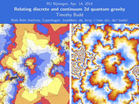
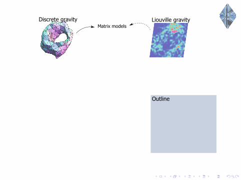
2D quantum gravity
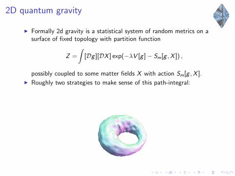
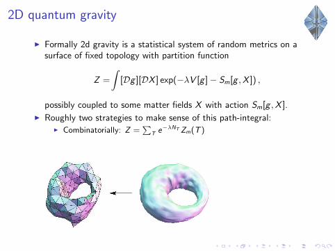
I Formally 2d gravity is a statistical system of random metrics on asurface of fixed topology with partition function
Z =
∫[Dg ][DX ] exp(−λV [g ]− Sm[g ,X ]) ,
possibly coupled to some matter fields X with action Sm[g ,X ].
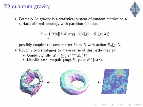
I Roughly two strategies to make sense of this path-integral:
I Combinatorially: Z =∑
T e−λNTZm(T )
I Liouville path integral: gauge fix gab = eγφgab(τ).
2D quantum gravity
I Formally 2d gravity is a statistical system of random metrics on asurface of fixed topology with partition function
Z =
∫[Dg ][DX ] exp(−λV [g ]− Sm[g ,X ]) ,
possibly coupled to some matter fields X with action Sm[g ,X ].
I Roughly two strategies to make sense of this path-integral:I Combinatorially: Z =
∑T e−λNTZm(T )
I Liouville path integral: gauge fix gab = eγφgab(τ).
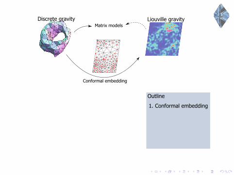
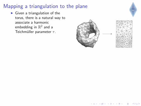
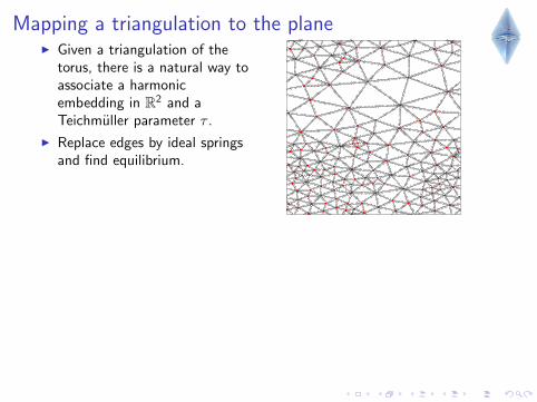
Mapping a triangulation to the planeI Given a triangulation of the
torus, there is a natural way toassociate a harmonicembedding in R2 and aTeichmuller parameter τ .
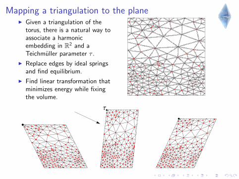
I Replace edges by ideal springsand find equilibrium.
I Find linear transformation thatminimizes energy while fixingthe volume.
Τ
Mapping a triangulation to the planeI Given a triangulation of the
torus, there is a natural way toassociate a harmonicembedding in R2 and aTeichmuller parameter τ .
I Replace edges by ideal springsand find equilibrium.
I Find linear transformation thatminimizes energy while fixingthe volume.
Τ
Mapping a triangulation to the planeI Given a triangulation of the
torus, there is a natural way toassociate a harmonicembedding in R2 and aTeichmuller parameter τ .
I Replace edges by ideal springsand find equilibrium.
I Find linear transformation thatminimizes energy while fixingthe volume.
Τ
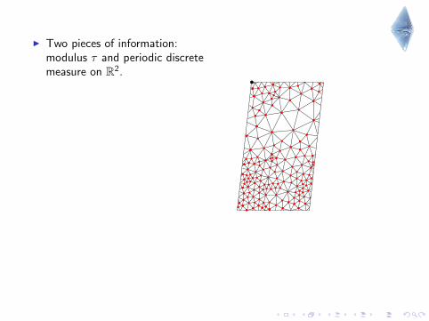
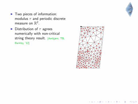
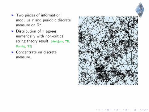
I Two pieces of information:modulus τ and periodic discretemeasure on R2.
I Distribution of τ agreesnumerically with non-criticalstring theory result. [Ambjørn, TB,
Barkley, ’12]
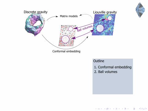
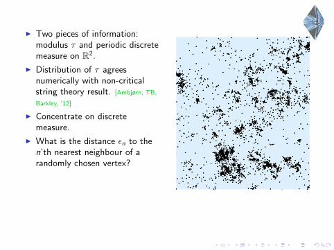
I Concentrate on discretemeasure.
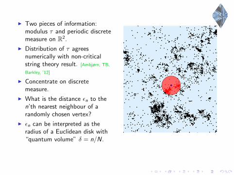
I What is the distance εn to then’th nearest neighbour of arandomly chosen vertex?
I εn can be interpreted as theradius of a Euclidean disk with“quantum volume” δ = n/N.
I Two pieces of information:modulus τ and periodic discretemeasure on R2.
I Distribution of τ agreesnumerically with non-criticalstring theory result. [Ambjørn, TB,
Barkley, ’12]
I Concentrate on discretemeasure.
I What is the distance εn to then’th nearest neighbour of arandomly chosen vertex?
I εn can be interpreted as theradius of a Euclidean disk with“quantum volume” δ = n/N.
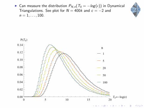
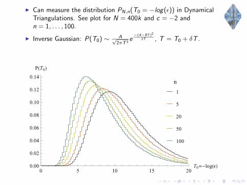
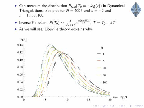
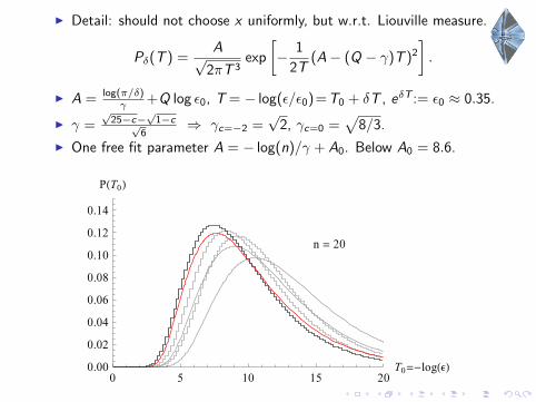
I Can measure the distribution PN,n(T0 = −log(ε)) in DynamicalTriangulations. See plot for N = 400k and c = −2 andn = 1, . . . , 100.
I Inverse Gaussian: P(T0) ∼ A√2πT 3
e−(A−BT )2
2T , T = T0 + δT .
I As we will see, Liouville theory explains why.
I Can measure the distribution PN,n(T0 = −log(ε)) in DynamicalTriangulations. See plot for N = 400k and c = −2 andn = 1, . . . , 100.
I Inverse Gaussian: P(T0) ∼ A√2πT 3
e−(A−BT )2
2T , T = T0 + δT .
I As we will see, Liouville theory explains why.
I Can measure the distribution PN,n(T0 = −log(ε)) in DynamicalTriangulations. See plot for N = 400k and c = −2 andn = 1, . . . , 100.
I Inverse Gaussian: P(T0) ∼ A√2πT 3
e−(A−BT )2
2T , T = T0 + δT .
I As we will see, Liouville theory explains why.
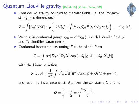
Quantum Liouville gravity [David, ’88] [Distler, Kawai, ’89]
I Consider 2d gravity coupled to c scalar fields, i.e. the Polyakovstring in c dimensions,
Z =
∫[Dg ][DX ] exp
(−λV [g ]−
∫d2x√gg ab∂aX
i∂bXjδij
), X ∈ Rc .
I Write g in conformal gauge gab = eγφgab(τ) with Liouville field φand Teichmuller parameter τ .
I Conformal bootstrap: assuming Z to be of the form
Z =
∫dτ [Dgφ][DgX ] exp (−SL[g , φ]− Sm[X , g ])
with the Liouville action
SL[g , φ] =1
4π
∫d2x
√g(g ab∂aφ∂bφ+ QRφ+ µeγφ)
and requiring invariance w.r.t. gab fixes the constants Q and γ:
Q =2
γ+γ
2=
√25− c
6
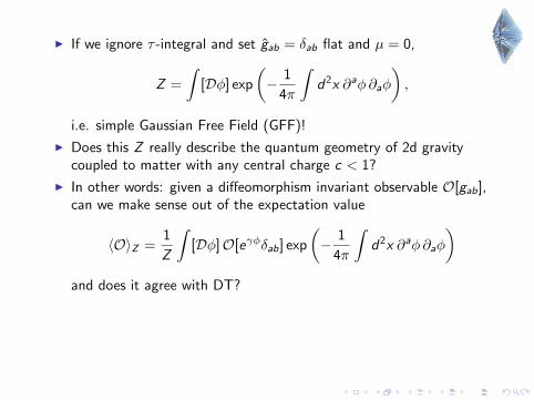
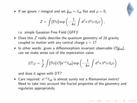
I If we ignore τ -integral and set gab = δab flat and µ = 0,
Z =
∫[Dφ] exp
(− 1
4π
∫d2x ∂aφ∂aφ
),
i.e. simple Gaussian Free Field (GFF)!
I Does this Z really describe the quantum geometry of 2d gravitycoupled to matter with any central charge c < 1?
I In other words: given a diffeomorphism invariant observable O[gab],can we make sense out of the expectation value
〈O〉Z =1
Z
∫[Dφ]O[eγφδab] exp
(− 1
4π
∫d2x ∂aφ∂aφ
)and does it agree with DT?
I Care required: eγφδab is almost surely not a Riemannian metric!Need to take into account the fractal properties of the geometry andregularize appropriately.
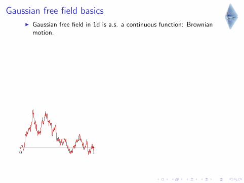
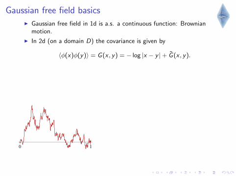
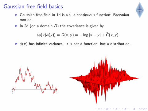
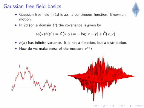
Gaussian free field basicsI Gaussian free field in 1d is a.s. a continuous function: Brownian
motion.
I In 2d (on a domain D) the covariance is given by
〈φ(x)φ(y)〉 = G (x , y) = − log |x − y |+ G (x , y).
I φ(x) has infinite variance. It is not a function, but a distribution.
I How do we make sense of the measure eγφ?
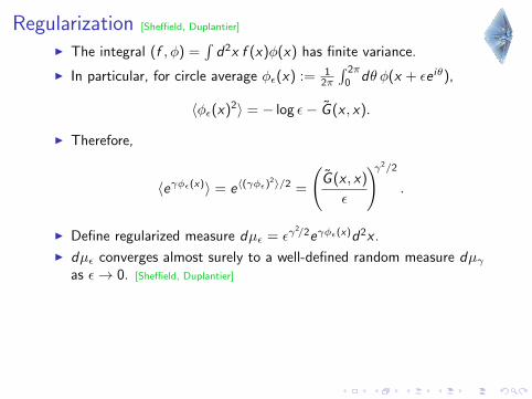
Regularization [Sheffield, Duplantier]
I The integral (f , φ) =∫d2x f (x)φ(x) has finite variance.
I In particular, for circle average φε(x) := 12π
∫ 2π
0dθ φ(x + εe iθ),
〈φε(x)2〉 = − log ε− G (x , x).
I Therefore,
〈eγφε(x)〉 = e〈(γφε)2〉/2 =
(G (x , x)
ε
)γ2/2
.
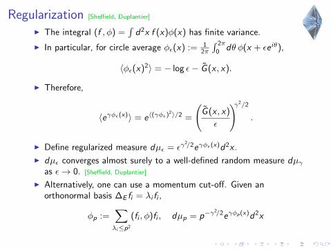
I Define regularized measure dµε = εγ2/2eγφε(x)d2x .
I dµε converges almost surely to a well-defined random measure dµγas ε→ 0. [Sheffield, Duplantier]
I Alternatively, one can use a momentum cut-off. Given anorthonormal basis ∆E fi = λi fi ,
φp :=∑λi≤p2
(fi , φ)fi , dµp = p−γ2/2eγφp(x)d2x
Regularization [Sheffield, Duplantier]
I The integral (f , φ) =∫d2x f (x)φ(x) has finite variance.
I In particular, for circle average φε(x) := 12π
∫ 2π
0dθ φ(x + εe iθ),
〈φε(x)2〉 = − log ε− G (x , x).
I Therefore,
〈eγφε(x)〉 = e〈(γφε)2〉/2 =
(G (x , x)
ε
)γ2/2
.
I Define regularized measure dµε = εγ2/2eγφε(x)d2x .
I dµε converges almost surely to a well-defined random measure dµγas ε→ 0. [Sheffield, Duplantier]
I Alternatively, one can use a momentum cut-off. Given anorthonormal basis ∆E fi = λi fi ,
φp :=∑λi≤p2
(fi , φ)fi , dµp = p−γ2/2eγφp(x)d2x
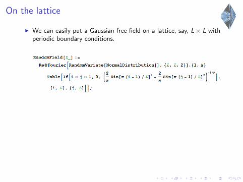
On the lattice
I We can easily put a Gaussian free field on a lattice, say, L× L withperiodic boundary conditions.
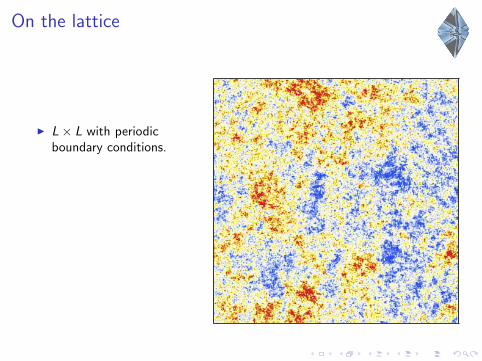
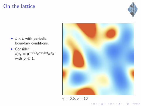
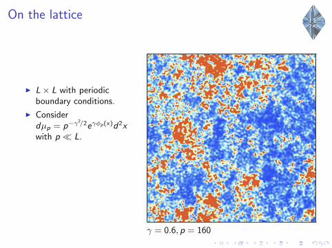
I L× L with periodicboundary conditions.
I Considerdµp = p−γ
2/2eγφp(x)d2xwith p � L.
I Can we understand therelation betweenδ = µ(Bε(x)) and ε?
On the lattice
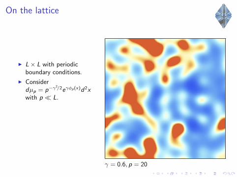
I L× L with periodicboundary conditions.
I Considerdµp = p−γ
2/2eγφp(x)d2xwith p � L.
I Can we understand therelation betweenδ = µ(Bε(x)) and ε?
p = 0
On the lattice
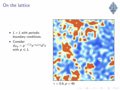
I L× L with periodicboundary conditions.
I Considerdµp = p−γ
2/2eγφp(x)d2xwith p � L.
I Can we understand therelation betweenδ = µ(Bε(x)) and ε?
γ = 0.6, p = 10
On the lattice
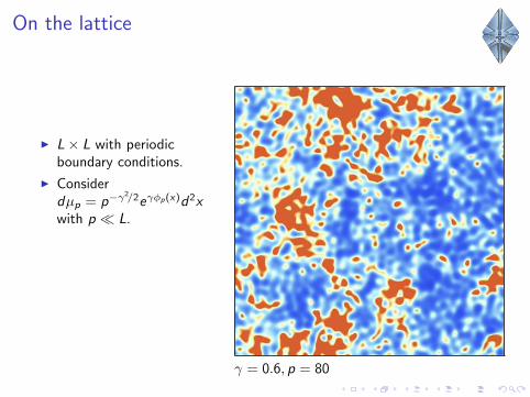
I L× L with periodicboundary conditions.
I Considerdµp = p−γ
2/2eγφp(x)d2xwith p � L.
I Can we understand therelation betweenδ = µ(Bε(x)) and ε?
γ = 0.6, p = 20
On the lattice
I L× L with periodicboundary conditions.
I Considerdµp = p−γ
2/2eγφp(x)d2xwith p � L.
I Can we understand therelation betweenδ = µ(Bε(x)) and ε?
γ = 0.6, p = 40
On the lattice
I L× L with periodicboundary conditions.
I Considerdµp = p−γ
2/2eγφp(x)d2xwith p � L.
I Can we understand therelation betweenδ = µ(Bε(x)) and ε?
γ = 0.6, p = 80
On the lattice
I L× L with periodicboundary conditions.
I Considerdµp = p−γ
2/2eγφp(x)d2xwith p � L.
I Can we understand therelation betweenδ = µ(Bε(x)) and ε?
γ = 0.6, p = 160

On the lattice
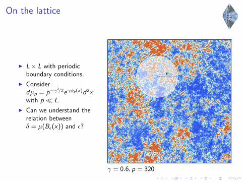
I L× L with periodicboundary conditions.
I Considerdµp = p−γ
2/2eγφp(x)d2xwith p � L.
I Can we understand therelation betweenδ = µ(Bε(x)) and ε?
γ = 0.6, p = 320
On the lattice
I L× L with periodicboundary conditions.
I Considerdµp = p−γ
2/2eγφp(x)d2xwith p � L.
I Can we understand therelation betweenδ = µ(Bε(x)) and ε?
γ = 0.6, p = 320
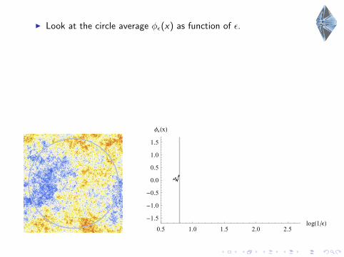
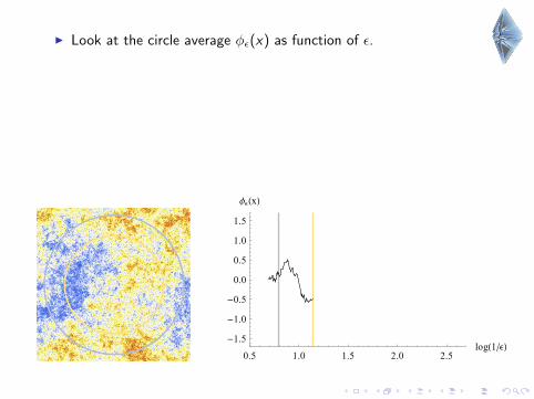
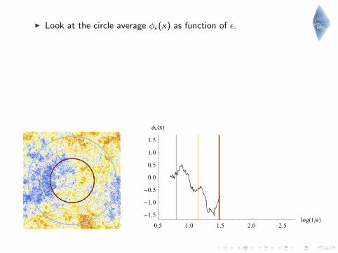
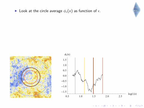
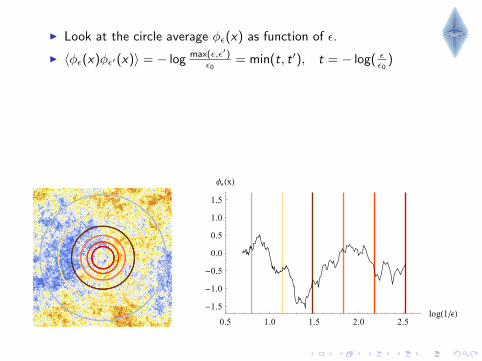
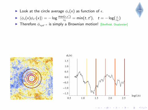
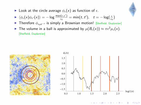
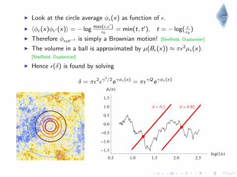
I Look at the circle average φε(x) as function of ε.
I 〈φε(x)φε′(x)〉 = − log max(ε,ε′)ε0
= min(t, t ′), t = − log( εε0)
I Therefore φε0e−t is simply a Brownian motion! [Sheffield, Duplantier]
I The volume in a ball is approximated by µ(Bε(x)) ≈ πε2µε(x).[Sheffield, Duplantier]
I Hence ε(δ) is found by solving
δ = πε2εγ2/2eγφε(x) = πεγQeγφε(x)
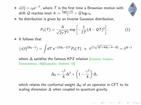
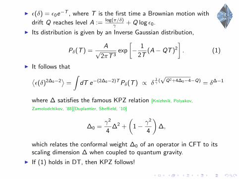
I ε(δ) = ε0e−T , where T is the first time a Brownian motion with
drift Q reaches level A := log(π/δ)γ + Q log ε0.
I Its distribution is given by an Inverse Gaussian distribution,
Pδ(T ) =A√
2πT 3exp
[− 1
2T(A− QT )2
]. (1)
I It follows that⟨ε(δ)2∆0−2
⟩=
∫dT e−(2∆0−2)TPδ(T ) ∝ δ
1γ (√
Q2+4∆0−4−Q) = δ∆−1
where ∆ satisfies the famous KPZ relation [Knizhnik, Polyakov,
Zamolodchikov, ’88][Duplantier, Sheffield, ’10]
∆0 =γ2
4∆2 +
(1− γ2
4
)∆,
which relates the conformal weight ∆0 of an operator in CFT to itsscaling dimension ∆ when coupled to quantum gravity.
I If (1) holds in DT, then KPZ follows!
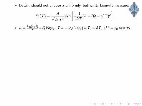
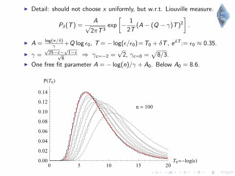
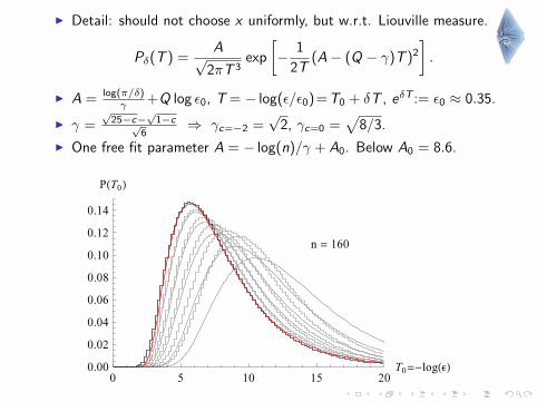
I Detail: should not choose x uniformly, but w.r.t. Liouville measure.
Pδ(T ) =A√
2πT 3exp
[− 1
2T(A− QT )2
].
I A = log(π/δ)γ +Q log ε0, T = − log(ε/ε0)=T0 + δT , eδT := ε0 ≈ 0.35.
I γ =√
25−c−√
1−c√6
⇒ γc=−2 =√
2, γc=0 =√
8/3.
I One free fit parameter A = − log(n)/γ + A0. Below A0 = 8.6.
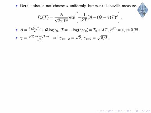
I Detail: should not choose x uniformly, but w.r.t. Liouville measure.
Pδ(T ) =A√
2πT 3exp
[− 1
2T(A− (Q − γ)T )2
].
I A = log(π/δ)γ +Q log ε0, T = − log(ε/ε0)=T0 + δT , eδT := ε0 ≈ 0.35.
I γ =√
25−c−√
1−c√6
⇒ γc=−2 =√
2, γc=0 =√
8/3.
I One free fit parameter A = − log(n)/γ + A0. Below A0 = 8.6.
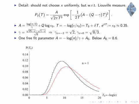
I Detail: should not choose x uniformly, but w.r.t. Liouville measure.
Pδ(T ) =A√
2πT 3exp
[− 1
2T(A− (Q − γ)T )2
].
I A = log(π/δ)γ +Q log ε0, T = − log(ε/ε0)=T0 + δT , eδT := ε0 ≈ 0.35.
I γ =√
25−c−√
1−c√6
⇒ γc=−2 =√
2, γc=0 =√
8/3.
I One free fit parameter A = − log(n)/γ + A0. Below A0 = 8.6.
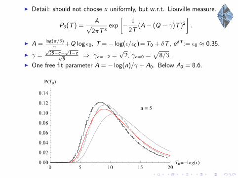
I Detail: should not choose x uniformly, but w.r.t. Liouville measure.
Pδ(T ) =A√
2πT 3exp
[− 1
2T(A− (Q − γ)T )2
].
I A = log(π/δ)γ +Q log ε0, T = − log(ε/ε0)=T0 + δT , eδT := ε0 ≈ 0.35.
I γ =√
25−c−√
1−c√6
⇒ γc=−2 =√
2, γc=0 =√
8/3.
I One free fit parameter A = − log(n)/γ + A0. Below A0 = 8.6.
I Detail: should not choose x uniformly, but w.r.t. Liouville measure.
Pδ(T ) =A√
2πT 3exp
[− 1
2T(A− (Q − γ)T )2
].
I A = log(π/δ)γ +Q log ε0, T = − log(ε/ε0)=T0 + δT , eδT := ε0 ≈ 0.35.
I γ =√
25−c−√
1−c√6
⇒ γc=−2 =√
2, γc=0 =√
8/3.
I One free fit parameter A = − log(n)/γ + A0. Below A0 = 8.6.
I Detail: should not choose x uniformly, but w.r.t. Liouville measure.
Pδ(T ) =A√
2πT 3exp
[− 1
2T(A− (Q − γ)T )2
].
I A = log(π/δ)γ +Q log ε0, T = − log(ε/ε0)=T0 + δT , eδT := ε0 ≈ 0.35.
I γ =√
25−c−√
1−c√6
⇒ γc=−2 =√
2, γc=0 =√
8/3.
I One free fit parameter A = − log(n)/γ + A0. Below A0 = 8.6.
I Detail: should not choose x uniformly, but w.r.t. Liouville measure.
Pδ(T ) =A√
2πT 3exp
[− 1
2T(A− (Q − γ)T )2
].
I A = log(π/δ)γ +Q log ε0, T = − log(ε/ε0)=T0 + δT , eδT := ε0 ≈ 0.35.
I γ =√
25−c−√
1−c√6
⇒ γc=−2 =√
2, γc=0 =√
8/3.
I One free fit parameter A = − log(n)/γ + A0. Below A0 = 8.6.

I Detail: should not choose x uniformly, but w.r.t. Liouville measure.
Pδ(T ) =A√
2πT 3exp
[− 1
2T(A− (Q − γ)T )2
].
I A = log(π/δ)γ +Q log ε0, T = − log(ε/ε0)=T0 + δT , eδT := ε0 ≈ 0.35.
I γ =√
25−c−√
1−c√6
⇒ γc=−2 =√
2, γc=0 =√
8/3.
I One free fit parameter A = − log(n)/γ + A0. Below A0 = 8.6.
I Detail: should not choose x uniformly, but w.r.t. Liouville measure.
Pδ(T ) =A√
2πT 3exp
[− 1
2T(A− (Q − γ)T )2
].
I A = log(π/δ)γ +Q log ε0, T = − log(ε/ε0)=T0 + δT , eδT := ε0 ≈ 0.35.
I γ =√
25−c−√
1−c√6
⇒ γc=−2 =√
2, γc=0 =√
8/3.
I One free fit parameter A = − log(n)/γ + A0. Below A0 = 8.6.
I Detail: should not choose x uniformly, but w.r.t. Liouville measure.
Pδ(T ) =A√
2πT 3exp
[− 1
2T(A− (Q − γ)T )2
].
I A = log(π/δ)γ +Q log ε0, T = − log(ε/ε0)=T0 + δT , eδT := ε0 ≈ 0.35.
I γ =√
25−c−√
1−c√6
⇒ γc=−2 =√
2, γc=0 =√
8/3.
I One free fit parameter A = − log(n)/γ + A0. Below A0 = 8.6.
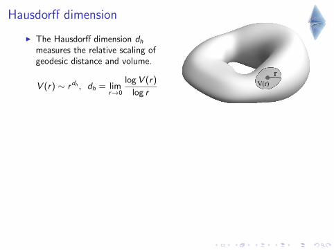
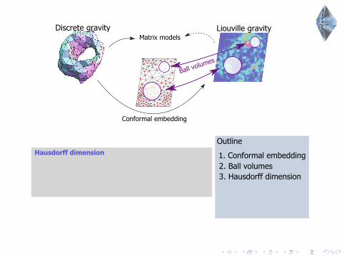
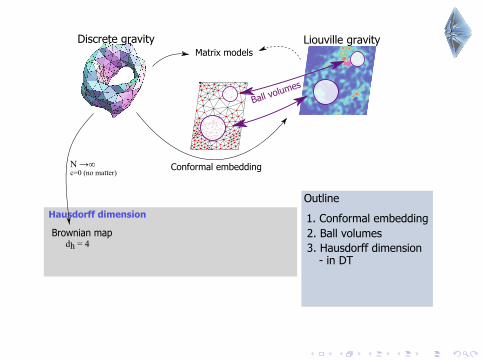
Hausdorff dimension
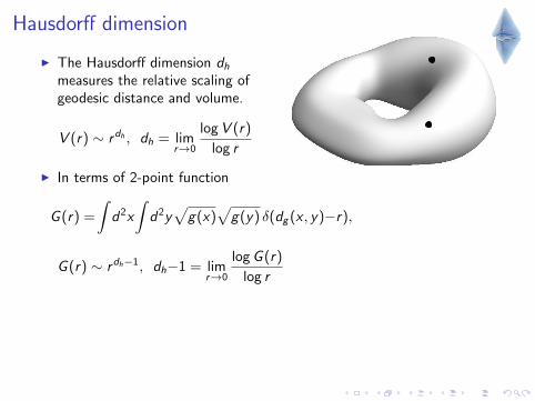
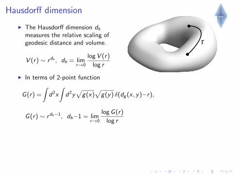
I The Hausdorff dimension dhmeasures the relative scaling ofgeodesic distance and volume.
V (r) ∼ rdh , dh = limr→0
logV (r)
log r
I In terms of 2-point function
G (r) =
∫d2x
∫d2y
√g(x)
√g(y) δ(dg (x , y)−r),
G (r) ∼ rdh−1, dh−1 = limr→0
logG (r)
log r
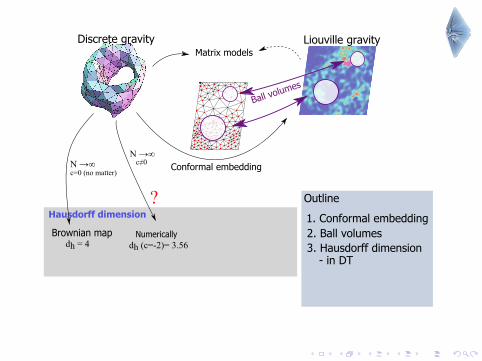
I For Riemannian surfaces dh = 2 but in random metrics we may finddh > 2. In fact, a typical geometry in pure 2d quantum gravity hasdh = 4.
Hausdorff dimension
I The Hausdorff dimension dhmeasures the relative scaling ofgeodesic distance and volume.
V (r) ∼ rdh , dh = limr→0
logV (r)
log r
I In terms of 2-point function
G (r) =
∫d2x
∫d2y
√g(x)
√g(y) δ(dg (x , y)−r),
G (r) ∼ rdh−1, dh−1 = limr→0
logG (r)
log r
I For Riemannian surfaces dh = 2 but in random metrics we may finddh > 2. In fact, a typical geometry in pure 2d quantum gravity hasdh = 4.
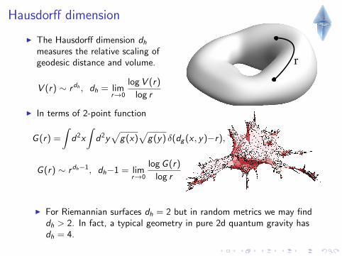
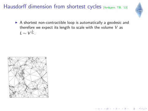
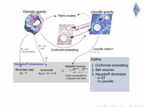
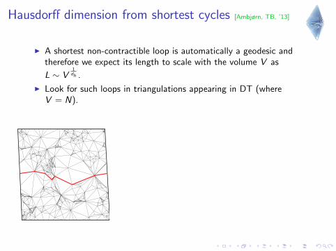
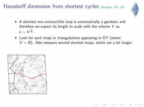
Hausdorff dimension from shortest cycles [Ambjørn, TB, ’13]
I A shortest non-contractible loop is automatically a geodesic andtherefore we expect its length to scale with the volume V as
L ∼ V1dh .
I Look for such loops in triangulations appearing in DT (whereV = N).
Also measure second shortest loops, which are a bit longer.
I Data agrees well with Watabiki’s formula: dh = 2√
49−c+√
25−c√25−c+
√1−c
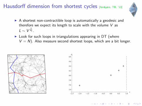
Hausdorff dimension from shortest cycles [Ambjørn, TB, ’13]
I A shortest non-contractible loop is automatically a geodesic andtherefore we expect its length to scale with the volume V as
L ∼ V1dh .
I Look for such loops in triangulations appearing in DT (whereV = N). Also measure second shortest loops, which are a bit longer.
I Data agrees well with Watabiki’s formula: dh = 2√
49−c+√
25−c√25−c+
√1−c
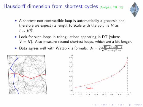
Hausdorff dimension from shortest cycles [Ambjørn, TB, ’13]
I A shortest non-contractible loop is automatically a geodesic andtherefore we expect its length to scale with the volume V as
L ∼ V1dh .
I Look for such loops in triangulations appearing in DT (whereV = N). Also measure second shortest loops, which are a bit longer.
I Data agrees well with Watabiki’s formula: dh = 2√
49−c+√
25−c√25−c+
√1−c
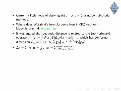
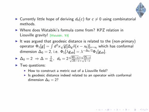
I Currently little hope of deriving dh(c) for c 6= 0 using combinatorialmethods.
I Where does Watabiki’s formula come from?
KPZ relation inLiouville gravity! [Watabiki, ’93]
I It was argued that geodesic distance is related to the (non-primary)operator Φ1[g ] =
∫d2x√g [∆gδ(x − x0)]x=x0 which has conformal
dimension ∆0 = 2, i.e. Φ1[λgab] = λ−∆0/2Φ1[gab].
I ∆0 = 2 ⇒ ∆ = 2dh, dh = 2
√49−c+
√25−c√
25−c+√
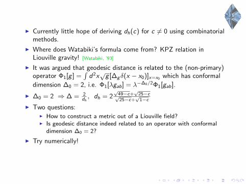
1−cI Two questions:
I How to construct a metric out of a Liouville field?I Is geodesic distance indeed related to an operator with conformal
dimension ∆0 = 2?
I Try numerically!
I Currently little hope of deriving dh(c) for c 6= 0 using combinatorialmethods.
I Where does Watabiki’s formula come from?
KPZ relation inLiouville gravity! [Watabiki, ’93]
I It was argued that geodesic distance is related to the (non-primary)operator Φ1[g ] =
∫d2x√g [∆gδ(x − x0)]x=x0 which has conformal
dimension ∆0 = 2, i.e. Φ1[λgab] = λ−∆0/2Φ1[gab].
I ∆0 = 2 ⇒ ∆ = 2dh, dh = 2
√49−c+
√25−c√
25−c+√
1−cI Two questions:
I How to construct a metric out of a Liouville field?I Is geodesic distance indeed related to an operator with conformal
dimension ∆0 = 2?
I Try numerically!
I Currently little hope of deriving dh(c) for c 6= 0 using combinatorialmethods.
I Where does Watabiki’s formula come from? KPZ relation inLiouville gravity! [Watabiki, ’93]
I It was argued that geodesic distance is related to the (non-primary)operator Φ1[g ] =
∫d2x√g [∆gδ(x − x0)]x=x0 which has conformal
dimension ∆0 = 2, i.e. Φ1[λgab] = λ−∆0/2Φ1[gab].
I ∆0 = 2 ⇒ ∆ = 2dh, dh = 2
√49−c+
√25−c√
25−c+√
1−c
I Two questions:I How to construct a metric out of a Liouville field?I Is geodesic distance indeed related to an operator with conformal
dimension ∆0 = 2?
I Try numerically!
I Currently little hope of deriving dh(c) for c 6= 0 using combinatorialmethods.
I Where does Watabiki’s formula come from? KPZ relation inLiouville gravity! [Watabiki, ’93]
I It was argued that geodesic distance is related to the (non-primary)operator Φ1[g ] =
∫d2x√g [∆gδ(x − x0)]x=x0 which has conformal
dimension ∆0 = 2, i.e. Φ1[λgab] = λ−∆0/2Φ1[gab].
I ∆0 = 2 ⇒ ∆ = 2dh, dh = 2
√49−c+
√25−c√
25−c+√
1−cI Two questions:
I How to construct a metric out of a Liouville field?I Is geodesic distance indeed related to an operator with conformal
dimension ∆0 = 2?
I Try numerically!
I Currently little hope of deriving dh(c) for c 6= 0 using combinatorialmethods.
I Where does Watabiki’s formula come from? KPZ relation inLiouville gravity! [Watabiki, ’93]
I It was argued that geodesic distance is related to the (non-primary)operator Φ1[g ] =
∫d2x√g [∆gδ(x − x0)]x=x0 which has conformal
dimension ∆0 = 2, i.e. Φ1[λgab] = λ−∆0/2Φ1[gab].
I ∆0 = 2 ⇒ ∆ = 2dh, dh = 2
√49−c+
√25−c√
25−c+√
1−cI Two questions:
I How to construct a metric out of a Liouville field?I Is geodesic distance indeed related to an operator with conformal
dimension ∆0 = 2?
I Try numerically!
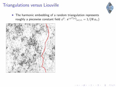
Triangulations versus Liouville
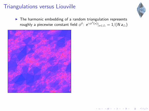
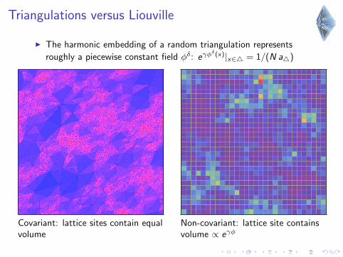
I The harmonic embedding of a random triangulation represents
roughly a piecewise constant field φδ: eγφδ(x)|x∈4 = 1/(N a4)
Covariant: lattice sites contain equalvolume
Non-covariant: lattice site containsvolume ∝ eγφ
Triangulations versus Liouville
I The harmonic embedding of a random triangulation represents
roughly a piecewise constant field φδ: eγφδ(x)|x∈4 = 1/(N a4)
Covariant: lattice sites contain equalvolume
Non-covariant: lattice site containsvolume ∝ eγφ
Triangulations versus Liouville
I The harmonic embedding of a random triangulation represents
roughly a piecewise constant field φδ: eγφδ(x)|x∈4 = 1/(N a4)
Covariant: lattice sites contain equalvolume
Non-covariant: lattice site containsvolume ∝ eγφ
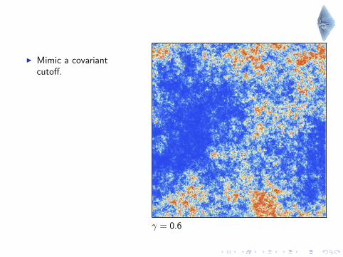
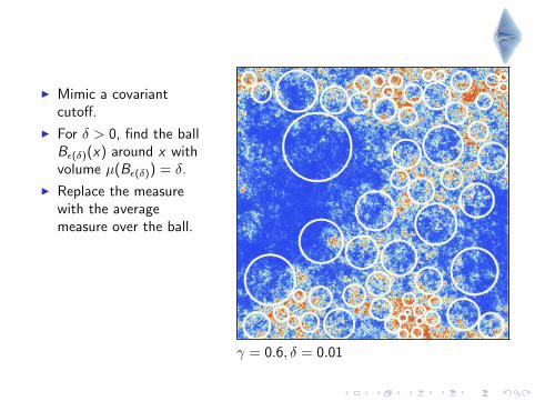
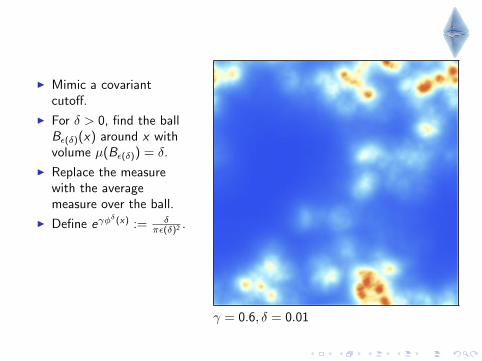
I Mimic a covariantcutoff.
I For δ > 0, find the ballBε(δ)(x) around x withvolume µ(Bε(δ)) = δ.
I Replace the measurewith the averagemeasure over the ball.
I Define eγφδ(x) := δ
πε(δ)2 .
I Compare to DT:δ ∼ 1/N
γ = 0.6
I Mimic a covariantcutoff.
I For δ > 0, find the ballBε(δ)(x) around x withvolume µ(Bε(δ)) = δ.
I Replace the measurewith the averagemeasure over the ball.
I Define eγφδ(x) := δ
πε(δ)2 .
I Compare to DT:δ ∼ 1/N
γ = 0.6, δ = 0.01
I Mimic a covariantcutoff.
I For δ > 0, find the ballBε(δ)(x) around x withvolume µ(Bε(δ)) = δ.
I Replace the measurewith the averagemeasure over the ball.
I Define eγφδ(x) := δ
πε(δ)2 .
I Compare to DT:δ ∼ 1/N
γ = 0.6, δ = 0.01
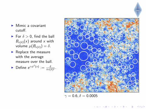
I Mimic a covariantcutoff.
I For δ > 0, find the ballBε(δ)(x) around x withvolume µ(Bε(δ)) = δ.
I Replace the measurewith the averagemeasure over the ball.
I Define eγφδ(x) := δ
πε(δ)2 .
I Compare to DT:δ ∼ 1/N
γ = 0.6, δ = 0.0005
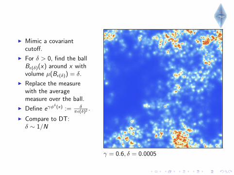
I Mimic a covariantcutoff.
I For δ > 0, find the ballBε(δ)(x) around x withvolume µ(Bε(δ)) = δ.
I Replace the measurewith the averagemeasure over the ball.
I Define eγφδ(x) := δ
πε(δ)2 .
I Compare to DT:δ ∼ 1/N
γ = 0.6, δ = 0.0005
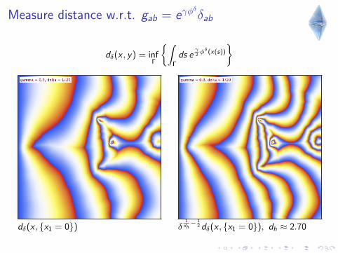
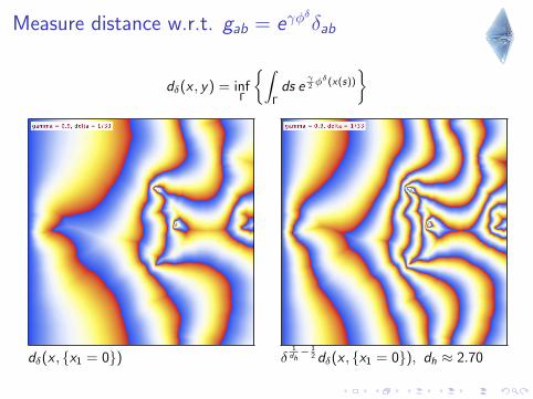
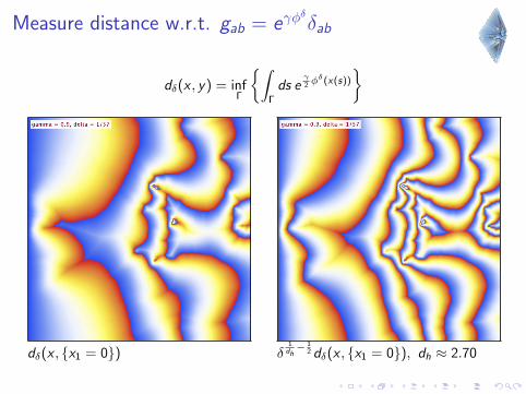
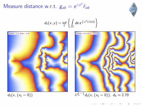
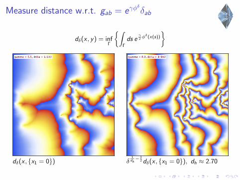
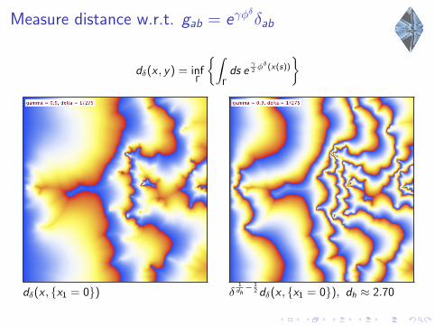
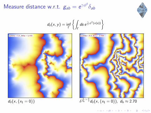
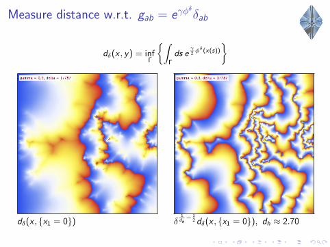
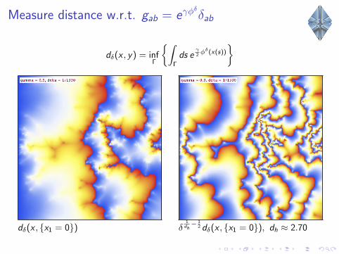
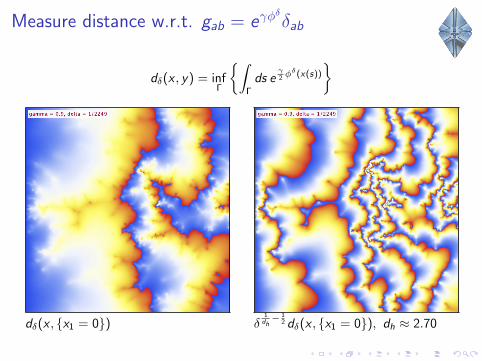
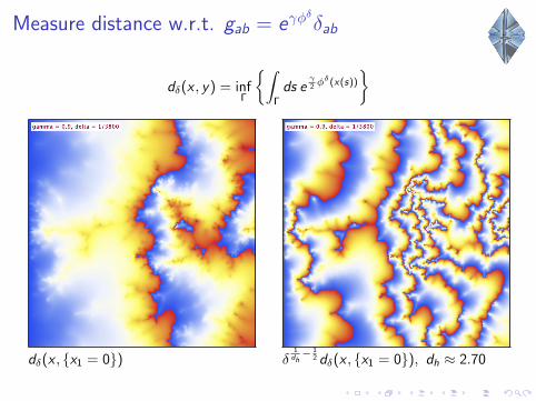
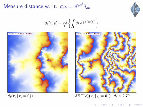
Measure distance w.r.t. gab = eγφδ
δab
dδ(x , y) = infΓ
{∫Γ
ds eγ2 φ
δ(x(s))
}
dδ(x , {x1 = 0}) δ1dh− 1
2 dδ(x , {x1 = 0}), dh ≈ 2.70
Measure distance w.r.t. gab = eγφδ
δab
dδ(x , y) = infΓ
{∫Γ
ds eγ2 φ
δ(x(s))
}
dδ(x , {x1 = 0}) δ1dh− 1
2 dδ(x , {x1 = 0}), dh ≈ 2.70
Measure distance w.r.t. gab = eγφδ
δab
dδ(x , y) = infΓ
{∫Γ
ds eγ2 φ
δ(x(s))
}
dδ(x , {x1 = 0}) δ1dh− 1
2 dδ(x , {x1 = 0}), dh ≈ 2.70
Measure distance w.r.t. gab = eγφδ
δab
dδ(x , y) = infΓ
{∫Γ
ds eγ2 φ
δ(x(s))
}
dδ(x , {x1 = 0}) δ1dh− 1
2 dδ(x , {x1 = 0}), dh ≈ 2.70
Measure distance w.r.t. gab = eγφδ
δab
dδ(x , y) = infΓ
{∫Γ
ds eγ2 φ
δ(x(s))
}
dδ(x , {x1 = 0}) δ1dh− 1
2 dδ(x , {x1 = 0}), dh ≈ 2.70
Measure distance w.r.t. gab = eγφδ
δab
dδ(x , y) = infΓ
{∫Γ
ds eγ2 φ
δ(x(s))
}
dδ(x , {x1 = 0}) δ1dh− 1
2 dδ(x , {x1 = 0}), dh ≈ 2.70
Measure distance w.r.t. gab = eγφδ
δab
dδ(x , y) = infΓ
{∫Γ
ds eγ2 φ
δ(x(s))
}
dδ(x , {x1 = 0}) δ1dh− 1
2 dδ(x , {x1 = 0}), dh ≈ 2.70
Measure distance w.r.t. gab = eγφδ
δab
dδ(x , y) = infΓ
{∫Γ
ds eγ2 φ
δ(x(s))
}
dδ(x , {x1 = 0}) δ1dh− 1
2 dδ(x , {x1 = 0}), dh ≈ 2.70
Measure distance w.r.t. gab = eγφδ
δab
dδ(x , y) = infΓ
{∫Γ
ds eγ2 φ
δ(x(s))
}
dδ(x , {x1 = 0}) δ1dh− 1
2 dδ(x , {x1 = 0}), dh ≈ 2.70
Measure distance w.r.t. gab = eγφδ
δab
dδ(x , y) = infΓ
{∫Γ
ds eγ2 φ
δ(x(s))
}
dδ(x , {x1 = 0}) δ1dh− 1
2 dδ(x , {x1 = 0}), dh ≈ 2.70
Measure distance w.r.t. gab = eγφδ
δab
dδ(x , y) = infΓ
{∫Γ
ds eγ2 φ
δ(x(s))
}
dδ(x , {x1 = 0}) δ1dh− 1
2 dδ(x , {x1 = 0}), dh ≈ 2.70
Measure distance w.r.t. gab = eγφδ
δab
dδ(x , y) = infΓ
{∫Γ
ds eγ2 φ
δ(x(s))
}
dδ(x , {x1 = 0}) δ1dh− 1
2 dδ(x , {x1 = 0}), dh ≈ 2.70
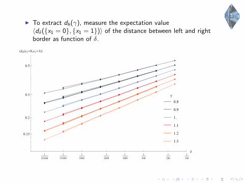
I To extract dh(γ), measure the expectation value〈dδ({x1 = 0}, {x1 = 1})〉 of the distance between left and rightborder as function of δ.
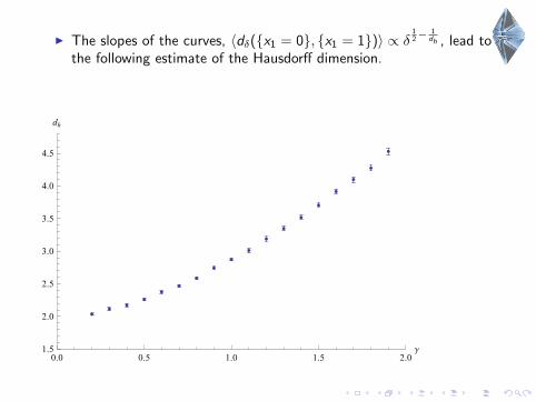
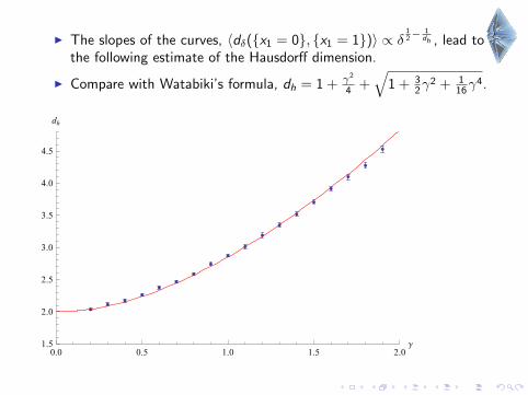
I The slopes of the curves, 〈dδ({x1 = 0}, {x1 = 1})〉 ∝ δ12−
1dh , lead to
the following estimate of the Hausdorff dimension.
I Compare with Watabiki’s formula, dh = 1 + γ2
4 +√
1 + 32γ
2 + 116γ
4.
I The slopes of the curves, 〈dδ({x1 = 0}, {x1 = 1})〉 ∝ δ12−
1dh , lead to
the following estimate of the Hausdorff dimension.
I Compare with Watabiki’s formula, dh = 1 + γ2
4 +√
1 + 32γ
2 + 116γ
4.
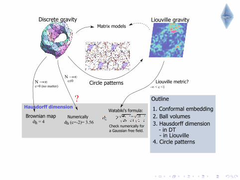
Circle patterns [David, Eynard, ’13]
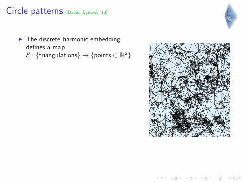
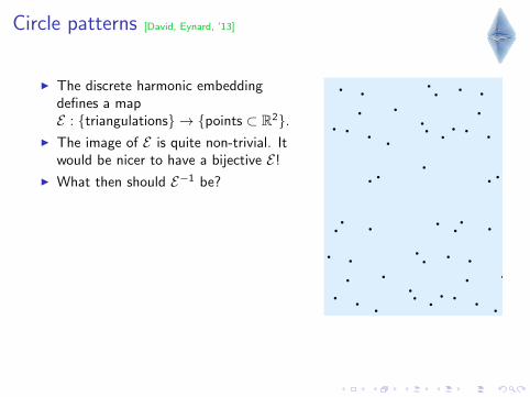
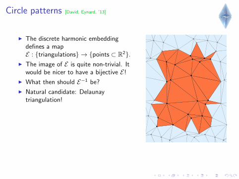
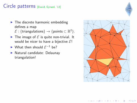
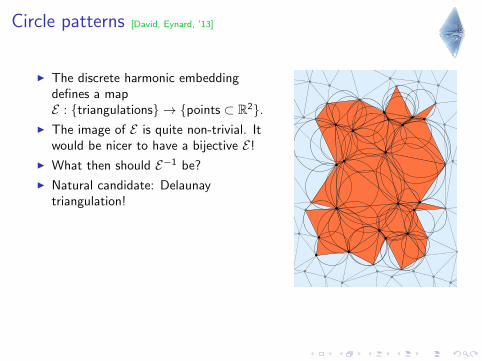
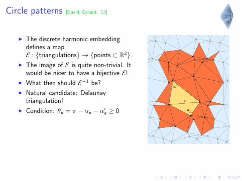
I The discrete harmonic embeddingdefines a mapE : {triangulations} → {points ⊂ R2}.
I The image of E is quite non-trivial. Itwould be nicer to have a bijective E!
I What then should E−1 be?
I Natural candidate: Delaunaytriangulation!
I Condition: θe = π − αe − α′e ≥ 0
I Circle pattern theorem [Rivin, ’94]: theembedding of the abstracttriangulation is uniquely determined bythe values {θe}.
Circle patterns [David, Eynard, ’13]
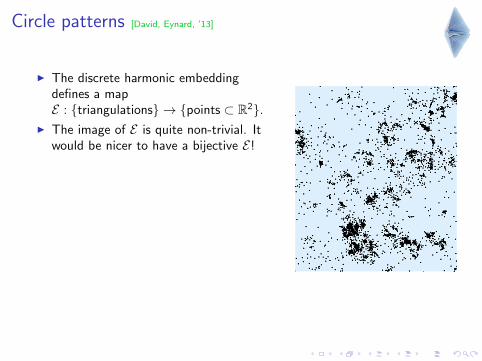
I The discrete harmonic embeddingdefines a mapE : {triangulations} → {points ⊂ R2}.
I The image of E is quite non-trivial. Itwould be nicer to have a bijective E!
I What then should E−1 be?
I Natural candidate: Delaunaytriangulation!
I Condition: θe = π − αe − α′e ≥ 0
I Circle pattern theorem [Rivin, ’94]: theembedding of the abstracttriangulation is uniquely determined bythe values {θe}.
Circle patterns [David, Eynard, ’13]
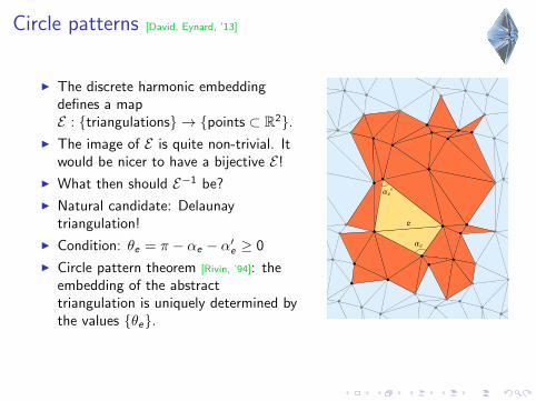
I The discrete harmonic embeddingdefines a mapE : {triangulations} → {points ⊂ R2}.
I The image of E is quite non-trivial. Itwould be nicer to have a bijective E!
I What then should E−1 be?
I Natural candidate: Delaunaytriangulation!
I Condition: θe = π − αe − α′e ≥ 0
I Circle pattern theorem [Rivin, ’94]: theembedding of the abstracttriangulation is uniquely determined bythe values {θe}.
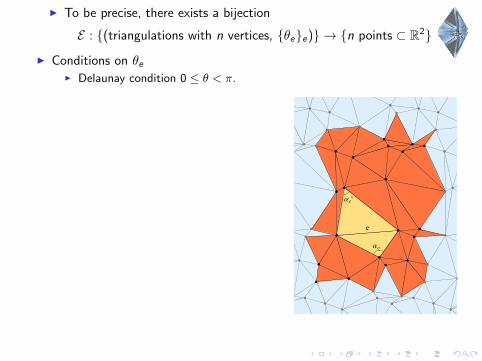
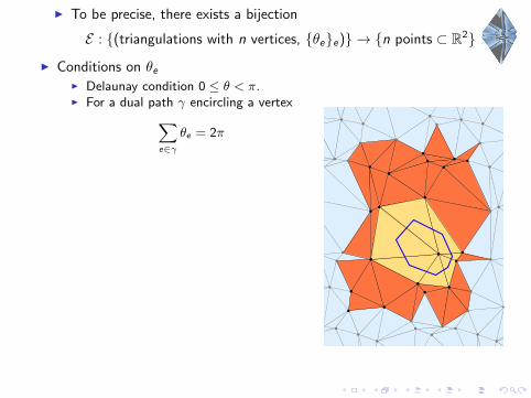
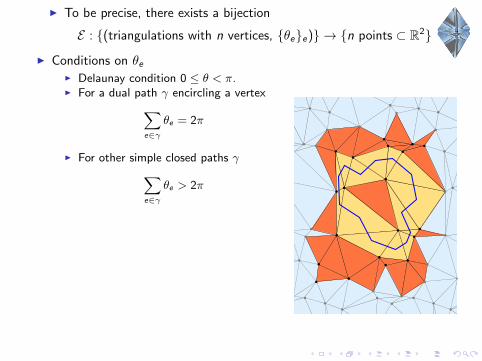
I To be precise, there exists a bijection
E : {(triangulations with n vertices, {θe}e)} → {n points ⊂ R2}
I Conditions on θeI Delaunay condition 0 ≤ θ < π.
I For a dual path γ encircling a vertex∑e∈γ
θe = 2π
I For other simple closed paths γ∑e∈γ
θe > 2π
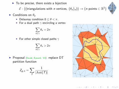
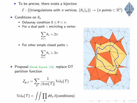
I Proposal [David, Eynard, ’13]: replace DTpartition function
Zg ,n =∑T
1
|Aut(T )|
Volθ(T )
Volθ(T ) =
∫ ∫ ∏e
dθe δ(conditions)
I To be precise, there exists a bijection
E : {(triangulations with n vertices, {θe}e)} → {n points ⊂ R2}
I Conditions on θeI Delaunay condition 0 ≤ θ < π.I For a dual path γ encircling a vertex∑
e∈γ
θe = 2π
I For other simple closed paths γ∑e∈γ
θe > 2π
I Proposal [David, Eynard, ’13]: replace DTpartition function
Zg ,n =∑T
1
|Aut(T )|Volθ(T )
Volθ(T ) =
∫ ∫ ∏e
dθe δ(conditions)
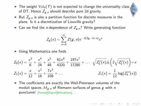
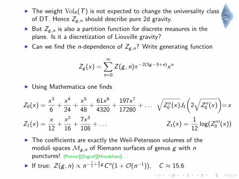
I The weight Volθ(T ) is not expected to change the universality classof DT. Hence Zg ,n should describe pure 2d gravity.
I But Zg ,n is also a partition function for discrete measures in theplane. Is it a discretization of Liouville gravity?
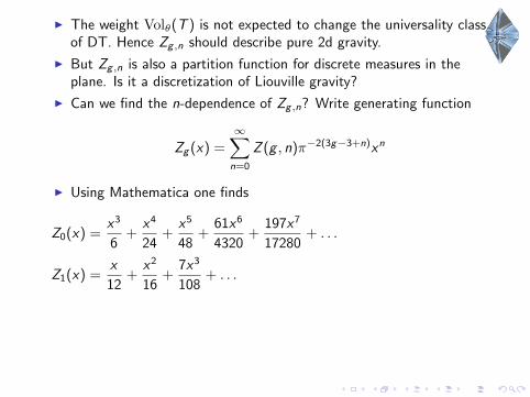
I Can we find the n-dependence of Zg ,n? Write generating function
Zg (x) =∞∑n=0
Z (g , n)π−2(3g−3+n)xn
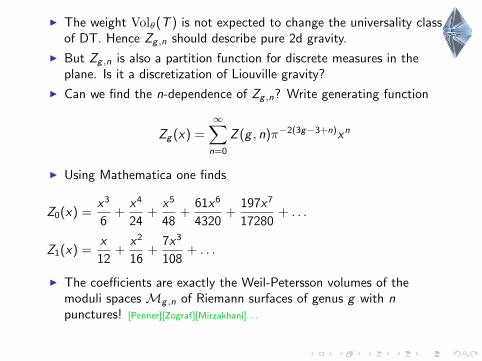
I Using Mathematica one finds
Z0(x) =x3
6+
x4
24+
x5
48+
61x6
4320+
197x7
17280+ . . .
√Z ′′0 (x)J1
(2√Z ′′0 (x)
)=x
Z1(x) =x
12+
x2
16+
7x3
108+ . . .
Z1(x) =1
12log(Z ′′′0 (x))
I The coefficients are exactly the Weil-Petersson volumes of themoduli spaces Mg ,n of Riemann surfaces of genus g with npunctures! [Penner][Zograf][Mirzakhani]. . .
I If true: Z (g , n) ∝ n−72 + 5
2 gC n(1 +O(n−1)), C ≈ 15.6
I The weight Volθ(T ) is not expected to change the universality classof DT. Hence Zg ,n should describe pure 2d gravity.
I But Zg ,n is also a partition function for discrete measures in theplane. Is it a discretization of Liouville gravity?
I Can we find the n-dependence of Zg ,n? Write generating function
Zg (x) =∞∑n=0
Z (g , n)π−2(3g−3+n)xn
I Using Mathematica one finds
Z0(x) =x3
6+
x4
24+
x5
48+
61x6
4320+
197x7
17280+ . . .
√Z ′′0 (x)J1
(2√
Z ′′0 (x)
)=x
Z1(x) =x
12+
x2
16+
7x3
108+ . . . Z1(x) =
1
12log(Z ′′′0 (x))
I The coefficients are exactly the Weil-Petersson volumes of themoduli spaces Mg ,n of Riemann surfaces of genus g with npunctures! [Penner][Zograf][Mirzakhani]. . .
I If true: Z (g , n) ∝ n−72 + 5
2 gC n(1 +O(n−1)), C ≈ 15.6
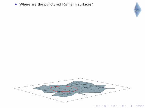
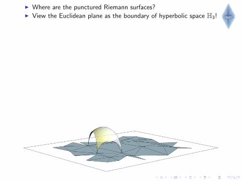
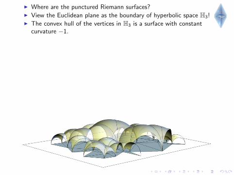
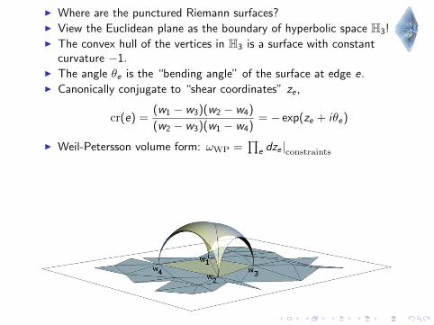
I Where are the punctured Riemann surfaces?
I View the Euclidean plane as the boundary of hyperbolic space H3!I The convex hull of the vertices in H3 is a surface with constant
curvature −1.I The angle θe is the “bending angle” of the surface at edge e.I Canonically conjugate to “shear coordinates” ze ,
cr(e) =(w1 − w3)(w2 − w4)
(w2 − w3)(w1 − w4)= − exp(ze + iθe)
I Weil-Petersson volume form: ωWP =∏
e dze |constraintsI Somehow the Delaunay conditions select a fundamental domain in
Teichmuller space.
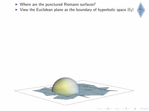
I Where are the punctured Riemann surfaces?I View the Euclidean plane as the boundary of hyperbolic space H3!
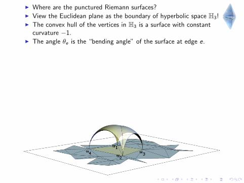
I The convex hull of the vertices in H3 is a surface with constantcurvature −1.
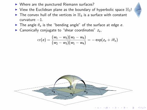
I The angle θe is the “bending angle” of the surface at edge e.I Canonically conjugate to “shear coordinates” ze ,
cr(e) =(w1 − w3)(w2 − w4)
(w2 − w3)(w1 − w4)= − exp(ze + iθe)
I Weil-Petersson volume form: ωWP =∏
e dze |constraintsI Somehow the Delaunay conditions select a fundamental domain in
Teichmuller space.
I Where are the punctured Riemann surfaces?I View the Euclidean plane as the boundary of hyperbolic space H3!
I The convex hull of the vertices in H3 is a surface with constantcurvature −1.
I The angle θe is the “bending angle” of the surface at edge e.I Canonically conjugate to “shear coordinates” ze ,
cr(e) =(w1 − w3)(w2 − w4)
(w2 − w3)(w1 − w4)= − exp(ze + iθe)
I Weil-Petersson volume form: ωWP =∏
e dze |constraintsI Somehow the Delaunay conditions select a fundamental domain in
Teichmuller space.
I Where are the punctured Riemann surfaces?I View the Euclidean plane as the boundary of hyperbolic space H3!I The convex hull of the vertices in H3 is a surface with constant
curvature −1.
I The angle θe is the “bending angle” of the surface at edge e.I Canonically conjugate to “shear coordinates” ze ,
cr(e) =(w1 − w3)(w2 − w4)
(w2 − w3)(w1 − w4)= − exp(ze + iθe)
I Weil-Petersson volume form: ωWP =∏
e dze |constraintsI Somehow the Delaunay conditions select a fundamental domain in
Teichmuller space.
I Where are the punctured Riemann surfaces?I View the Euclidean plane as the boundary of hyperbolic space H3!I The convex hull of the vertices in H3 is a surface with constant
curvature −1.I The angle θe is the “bending angle” of the surface at edge e.
I Canonically conjugate to “shear coordinates” ze ,
cr(e) =(w1 − w3)(w2 − w4)
(w2 − w3)(w1 − w4)= − exp(ze + iθe)
I Weil-Petersson volume form: ωWP =∏
e dze |constraintsI Somehow the Delaunay conditions select a fundamental domain in
Teichmuller space.
I Where are the punctured Riemann surfaces?I View the Euclidean plane as the boundary of hyperbolic space H3!I The convex hull of the vertices in H3 is a surface with constant
curvature −1.I The angle θe is the “bending angle” of the surface at edge e.I Canonically conjugate to “shear coordinates” ze ,
cr(e) =(w1 − w3)(w2 − w4)
(w2 − w3)(w1 − w4)= − exp(ze + iθe)
I Weil-Petersson volume form: ωWP =∏
e dze |constraintsI Somehow the Delaunay conditions select a fundamental domain in
Teichmuller space.
I Where are the punctured Riemann surfaces?I View the Euclidean plane as the boundary of hyperbolic space H3!I The convex hull of the vertices in H3 is a surface with constant
curvature −1.I The angle θe is the “bending angle” of the surface at edge e.I Canonically conjugate to “shear coordinates” ze ,
cr(e) =(w1 − w3)(w2 − w4)
(w2 − w3)(w1 − w4)= − exp(ze + iθe)
I Weil-Petersson volume form: ωWP =∏
e dze |constraints
I Somehow the Delaunay conditions select a fundamental domain inTeichmuller space.

I Where are the punctured Riemann surfaces?I View the Euclidean plane as the boundary of hyperbolic space H3!I The convex hull of the vertices in H3 is a surface with constant
curvature −1.I The angle θe is the “bending angle” of the surface at edge e.I Canonically conjugate to “shear coordinates” ze ,
cr(e) =(w1 − w3)(w2 − w4)
(w2 − w3)(w1 − w4)= − exp(ze + iθe)
I Weil-Petersson volume form: ωWP =∏
e dze |constraintsI Somehow the Delaunay conditions select a fundamental domain in
Teichmuller space.
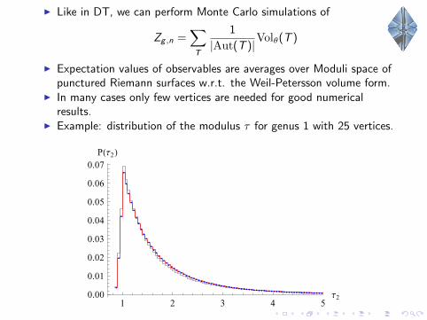
I Like in DT, we can perform Monte Carlo simulations of
Zg ,n =∑T
1
|Aut(T )|Volθ(T )
I Expectation values of observables are averages over Moduli space ofpunctured Riemann surfaces w.r.t. the Weil-Petersson volume form.
I In many cases only few vertices are needed for good numericalresults.
I Example: distribution of the modulus τ for genus 1 with 25 vertices.
Summary & outlookI Summary
I By a discrete conformal mapping one can assign a discrete measureto a random triangulation. This random measure is shownnumerically to share properties with the measure in QuantumLiouville gravity.
I Conversely, one can assign a geometric interpretation to a Liouvillemeasure by implementing a covariant cut-off. This is used tomeasure the Hausdorff dimension, which agrees well with Watabiki’sformula.
I Circle patterns give a more precise conformal mapping betweentriangulations and discrete measures and reveal a close connectionwith the well-studied Weil-Petersson geometry of Riemann surfaces.
I Outlook
I Make sense of the derivation of Watabiki’s Hausdorff dimension.I Until now we have only looked at Gaussian Free Fields instead of real
Liouville fields. Can we understand conformal correlation functions?I What can one compute analytically using circle patterns? Various
Weil-Petersson volumes have been calculated in the mathematicalliterature, but to what observable do they correspond?
Thanks! Questions? Slides available at http://www.nbi.dk/~budd/
Summary & outlookI Summary
I By a discrete conformal mapping one can assign a discrete measureto a random triangulation. This random measure is shownnumerically to share properties with the measure in QuantumLiouville gravity.
I Conversely, one can assign a geometric interpretation to a Liouvillemeasure by implementing a covariant cut-off. This is used tomeasure the Hausdorff dimension, which agrees well with Watabiki’sformula.
I Circle patterns give a more precise conformal mapping betweentriangulations and discrete measures and reveal a close connectionwith the well-studied Weil-Petersson geometry of Riemann surfaces.
I OutlookI Make sense of the derivation of Watabiki’s Hausdorff dimension.
I Until now we have only looked at Gaussian Free Fields instead of realLiouville fields. Can we understand conformal correlation functions?
I What can one compute analytically using circle patterns? VariousWeil-Petersson volumes have been calculated in the mathematicalliterature, but to what observable do they correspond?
Thanks! Questions? Slides available at http://www.nbi.dk/~budd/
Summary & outlookI Summary
I By a discrete conformal mapping one can assign a discrete measureto a random triangulation. This random measure is shownnumerically to share properties with the measure in QuantumLiouville gravity.
I Conversely, one can assign a geometric interpretation to a Liouvillemeasure by implementing a covariant cut-off. This is used tomeasure the Hausdorff dimension, which agrees well with Watabiki’sformula.
I Circle patterns give a more precise conformal mapping betweentriangulations and discrete measures and reveal a close connectionwith the well-studied Weil-Petersson geometry of Riemann surfaces.
I OutlookI Make sense of the derivation of Watabiki’s Hausdorff dimension.I Until now we have only looked at Gaussian Free Fields instead of real
Liouville fields. Can we understand conformal correlation functions?
I What can one compute analytically using circle patterns? VariousWeil-Petersson volumes have been calculated in the mathematicalliterature, but to what observable do they correspond?
Thanks! Questions? Slides available at http://www.nbi.dk/~budd/
Summary & outlookI Summary
I By a discrete conformal mapping one can assign a discrete measureto a random triangulation. This random measure is shownnumerically to share properties with the measure in QuantumLiouville gravity.
I Conversely, one can assign a geometric interpretation to a Liouvillemeasure by implementing a covariant cut-off. This is used tomeasure the Hausdorff dimension, which agrees well with Watabiki’sformula.
I Circle patterns give a more precise conformal mapping betweentriangulations and discrete measures and reveal a close connectionwith the well-studied Weil-Petersson geometry of Riemann surfaces.
I OutlookI Make sense of the derivation of Watabiki’s Hausdorff dimension.I Until now we have only looked at Gaussian Free Fields instead of real
Liouville fields. Can we understand conformal correlation functions?I What can one compute analytically using circle patterns? Various
Weil-Petersson volumes have been calculated in the mathematicalliterature, but to what observable do they correspond?
Thanks! Questions? Slides available at http://www.nbi.dk/~budd/
Summary & outlookI Summary
I By a discrete conformal mapping one can assign a discrete measureto a random triangulation. This random measure is shownnumerically to share properties with the measure in QuantumLiouville gravity.
I Conversely, one can assign a geometric interpretation to a Liouvillemeasure by implementing a covariant cut-off. This is used tomeasure the Hausdorff dimension, which agrees well with Watabiki’sformula.
I Circle patterns give a more precise conformal mapping betweentriangulations and discrete measures and reveal a close connectionwith the well-studied Weil-Petersson geometry of Riemann surfaces.
I OutlookI Make sense of the derivation of Watabiki’s Hausdorff dimension.I Until now we have only looked at Gaussian Free Fields instead of real
Liouville fields. Can we understand conformal correlation functions?I What can one compute analytically using circle patterns? Various
Weil-Petersson volumes have been calculated in the mathematicalliterature, but to what observable do they correspond?
Thanks! Questions? Slides available at http://www.nbi.dk/~budd/


![Unraveling conformal gravity amplitudesgravity.psu.edu › events › superstring_supergravity › talks › mogull_sstu2018.pdfUnraveling conformal gravity amplitudes based on [1806.05124]](https://static.fdocument.org/doc/165x107/5f0cfc827e708231d4381d0d/unraveling-conformal-gravity-a-events-a-superstringsupergravity-a-talks-a.jpg)