Regressão Linear e MultilinearDelineamento ExperimentalMestrado em Sistemas de Produção em Agricultura Mediterrânica

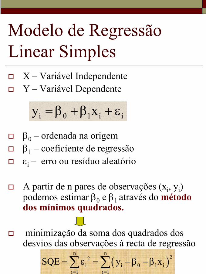
Modelo de Regressão Linear Simples

X – Variável IndependenteY – Variável Dependente

β0 – ordenada na origemβ1 – coeficiente de regressãoεi – erro ou resíduo aleatório

A partir de n pares de observações (xi, yi) podemos estimar β0 e β1 através do método dos mínimos quadrados.

minimização da soma dos quadrados dos desvios das observações à recta de regressão

i 0 1 i iy x= β +β + ε

( )n n

22i i 0 1 i

i 1 i 1SQE y x

= =

= ε = −β −β∑ ∑

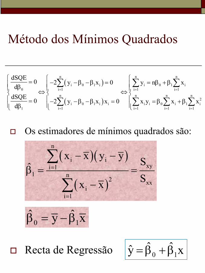
Método dos Mínimos Quadrados

Os estimadores de mínimos quadrados são:

Recta de Regressão

( )

( )

n n n

i 0 1 i i 0 1 i0 i 1 i 1 i 1

n n n n2

i 0 1 i i i i 0 i 1 ii 1 i 1 i 1 i 11

dSQE 0 2 y x 0 y n xd

dSQE 0 2 y x x 0 x y x xd

= = =

= = = =

= − −β −β = = β +β β ⇔ ⇔ = − −β −β = = β +β β

∑ ∑ ∑

∑ ∑ ∑ ∑

( )( )

( )

n

i ixyi 1

1 n2 xx

ii 1

x x y y SˆSx x

=

=

− −β = =

−

∑

∑

0 1ˆ ˆy xβ = −β

0 1ˆ ˆy x= β +β

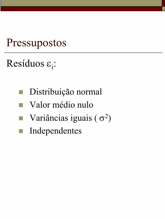
Pressupostos

Resíduos εi:

Distribuição normalValor médio nuloVariâncias iguais ( σ2)Independentes

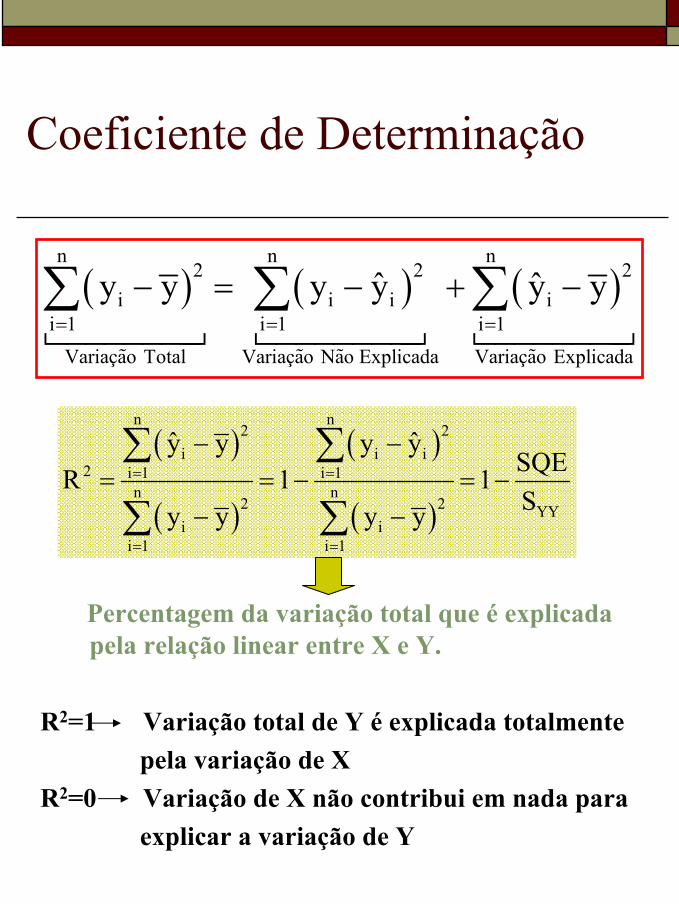
Coeficiente de Determinação

Percentagem da variação total que é explicada pela relação linear entre X e Y.

R2=1 Variação total de Y é explicada totalmente pela variação de X

R2=0 Variação de X não contribui em nada paraexplicar a variação de Y

( ) ( ) ( )n n n

2 2 2i i i i

i 1 i 1 i 1Variaçao Total Variaçao Nao Explicada Variaçao Explicada

ˆ ˆy y y y y y= = =

− = − + −∑ ∑ ∑

( )

( )

( )

( )

n n2 2

i i i2 i 1 i 1

n n2 2 YY

i ii 1 i 1

ˆ ˆy y y ySQER 1 1Sy y y y

= =

= =

− −= = − = −

− −

∑ ∑

∑ ∑

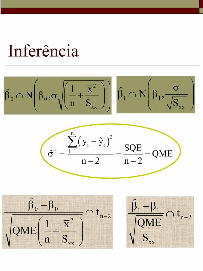
Inferência

2

0 0xx

1 xˆ N ,n S

β ∩ β σ + 1 1

xx

ˆ N ,S

σβ ∩ β

( )n

2i i

2 i 1

ˆy ySQEˆ QME

n 2 n 2=

−σ = = =

− −

∑

0 0n 2

2

xx

ˆt

1 xQMEn S

−

β −β∩

+

1 1n 2

xx

ˆt

QMES

−

β −β∩

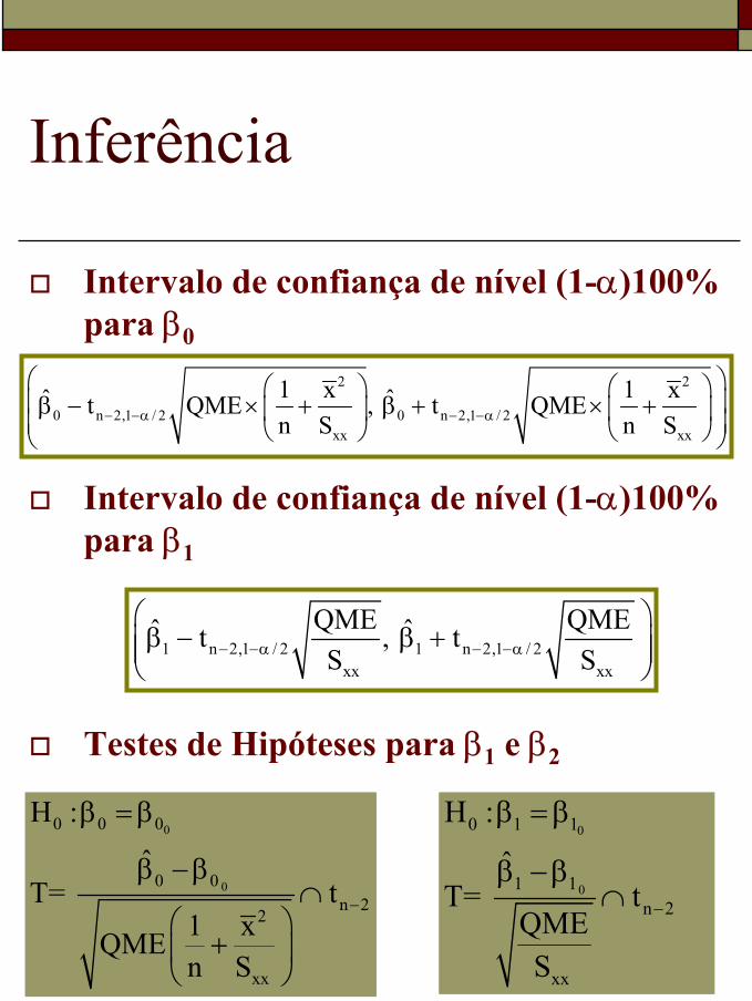
Inferência

Intervalo de confiança de nível (1-α)100% para β0

Intervalo de confiança de nível (1-α)100% para β1

Testes de Hipóteses para β1 e β2

2 2

0 n 2,1 / 2 0 n 2,1 / 2xx xx

1 x 1 xˆ ˆt QME , t QMEn S n S− −α − −α

β − × + β + × +

1 n 2,1 / 2 1 n 2,1 / 2xx xx

QME QMEˆ ˆt , tS S− −α − −α

β − β +

0

0

0 0 0

0 0n 2

2

xx

H : ˆ

T= t1 xQMEn S

−

β = β

β −β∩

+

0

0

0 1 1

1 1n 2

xx

H : ˆ

T= tQMES

−

β = β

β −β∩

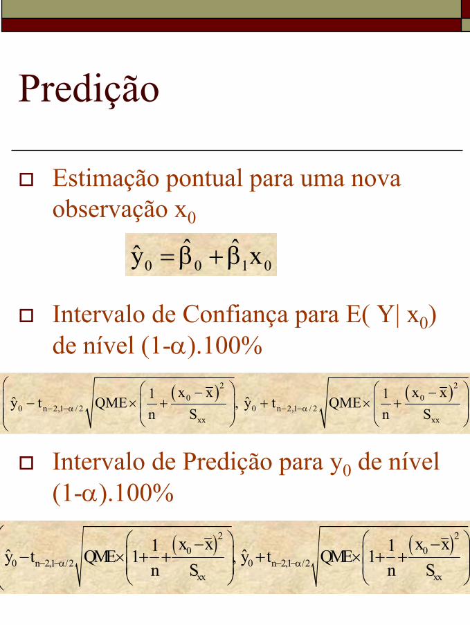
Predição

Estimação pontual para uma nova observação x0

Intervalo de Confiança para E( Y| x0) de nível (1-α).100%

Intervalo de Predição para y0 de nível (1-α).100%

0 0 1 0ˆ ˆy x= β +β

( ) ( )2 20 0

0 n 2,1 /2 0 n 2,1 /2xx xx

x x x x1 1ˆ ˆy t QME 1 , y t QME 1n S n S− −α − −α

− − − × + + + × + +

( ) ( )2 20 0

0 n 2,1 / 2 0 n 2,1 / 2xx xx

x x x x1 1ˆ ˆy t QME , y t QMEn S n S− −α − −α

− − − × + + × +

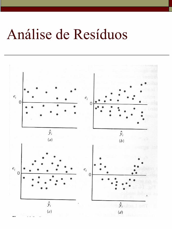
Análise de Resíduos

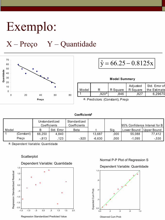
Exemplo:X – Preço Y – Quantidade

0

10

20

30

40

50

60

70

0 20 40 60 80

Preço

Qua

ntid

ade

y 66.25 0.8125x= −

Model Summary

,920a ,846 ,827 6,29670Model1

R R SquareAdjustedR Square

Std. Error ofthe Estimate

Predictors: (Constant), Preçoa.

Coefficientsa

66,250 4,840 13,687 ,000 55,088 77,412-,813 ,123 -,920 -6,630 ,000 -1,095 -,530

(Constant)Preço

Model1

B Std. Error

UnstandardizedCoefficients

Beta

StandardizedCoefficients

t Sig. Lower Bound Upper Bound95% Confidence Interval for B

Dependent Variable: Quantidadea.

Scatterplot

Dependent Variable: Quantidade

Regression Standardized Predicted Value

2,01,51,0,50,0-,5-1,0-1,5

Reg

ress

ion

Sta

ndar

dize

d R

esid

ual

1,5

1,0

,5

0,0

-,5

-1,0

-1,5

-2,0

Normal P-P Plot of Regression St

Dependent Variable: Quantidade

Observed Cum Prob

1,0,8,5,30,0

Exp

ecte

d C

um P

rob

1,0

,8

,5

,3

0,0

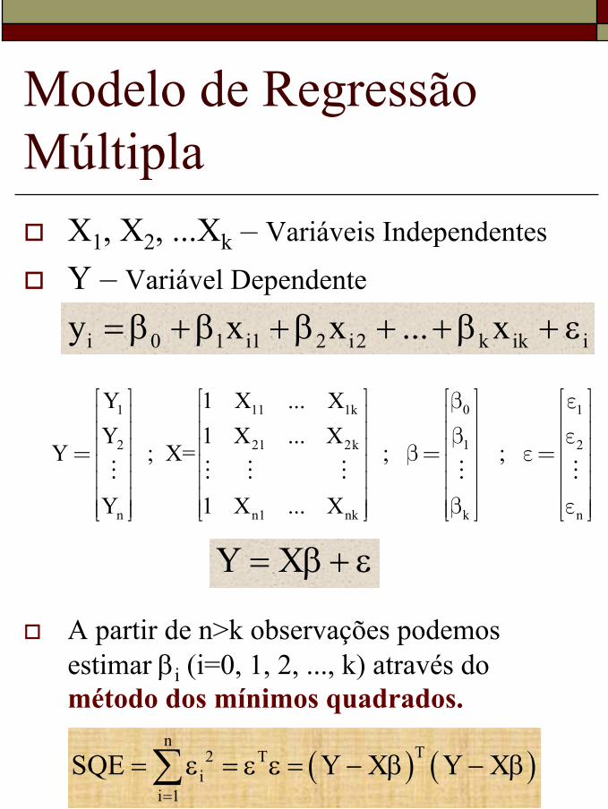
Modelo de Regressão Múltipla

X1, X2, ...Xk – Variáveis Independentes

Y – Variável Dependente

A partir de n>k observações podemos estimar βi (i=0, 1, 2, ..., k) através do método dos mínimos quadrados.

i 0 1 i1 2 i2 k ik iy x x ... x= β +β +β + +β + ε

( ) ( )n

T2 Ti

i 1SQE Y X Y X

=

= ε = ε ε = − β − β∑

1 11 1k 0 1

2 21 2k 1 2

n n1 nk k n

Y 1 X ... XY 1 X ... X

Y ; X= ; ;

Y 1 X ... X

β ε β ε = β= ε= β ε

Y X= β + ε

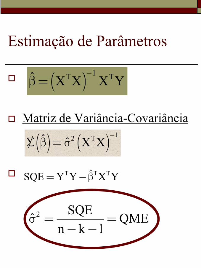
Estimação de Parâmetros

Matriz de Variância-Covariância

( ) 1T Tˆ X X X Y−

β=

( ) ( ) 12 Tˆ ˆ X X−/Σ β = σ

T T TˆSQE Y Y X Y= −β

2 SQEˆ QMEn k 1

σ = =− −

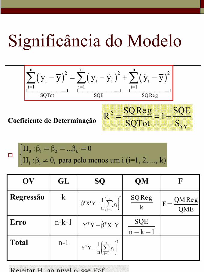
Significância do Modelo

Coeficiente de Determinação

( ) ( ) ( )n n n

2 2 2i i i i

i 1 i 1 i 1SQTot SQE SQReg

ˆ ˆy y y y y y= = =

− = − + −∑ ∑ ∑

2

YY

SQReg SQER 1SQTot S

= = −

0 1 2 k

1 i

H : ... 0H : 0, para pelo menos um i (i=1, 2, ..., k)

β = β = β = β ≠

n-1Total

n-k-1Erro

kRegressão

FQMSQGLOV

2nT T

ii 1

1ˆ X Y yn =

β − ∑

T T TˆY Y X Y−β

2nT

ii 1

1Y Y yn =

− ∑

QM RegFQME

=SQReg

k

SQEn k 1− −

0 k, n-k-1, 1-Rejeitar H ao nivel sse F>f αα

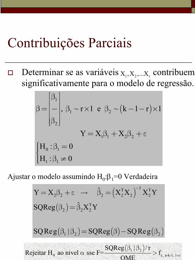
Contribuições Parciais

Determinar se as variáveis contribuem significativamente para o modelo de regressão.

Ajustar o modelo assumindo H0:β1=0 Verdadeira

1 2 rX ,X ,...X

( )1

1 2

2

1 1 2 2

0 1

1 1

, ~ r 1 e ~ k 1 r 1

Y X XH : 0H : 0

β β= − β × β − − × β

= β + β + ε β = β ≠

( )( )

( ) ( ) ( )

1T T2 2 2 2 2 2

T2 2 2

1 2 2

ˆY X X X X Y

ˆSQReg X Y

SQReg | SQReg SQReg

−= β + ε → β =

β = β

β β = β − β

( )1 20 r, n-k-1, 1-

SQReg | / rRejeitar H ao nivel sse F= f

QME α

β βα >

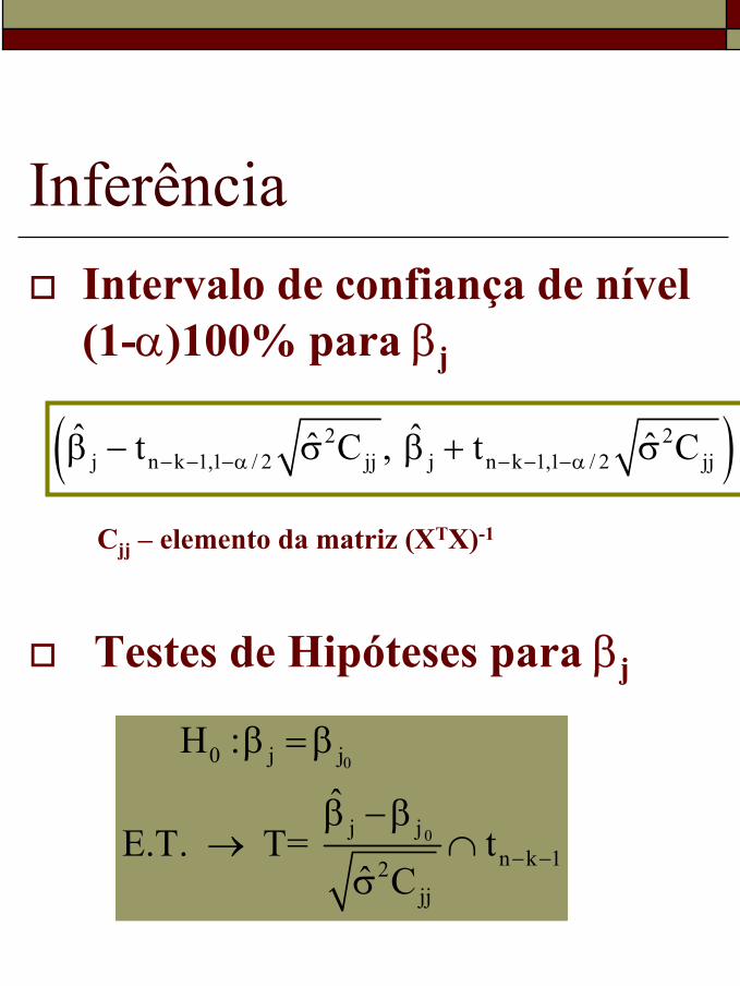
InferênciaIntervalo de confiança de nível (1-α)100% para βj

Cjj – elemento da matriz (XTX)-1

Testes de Hipóteses para βj

( )2 2j n k 1,1 / 2 jj j n k 1,1 / 2 jj

ˆ ˆˆ ˆt C , t C− − −α − − −αβ − σ β + σ

0

0

0 j j

j jn k 12

jj

H : ˆ

E.T. T= tˆ C

− −

β = β

β −β→ ∩

σ

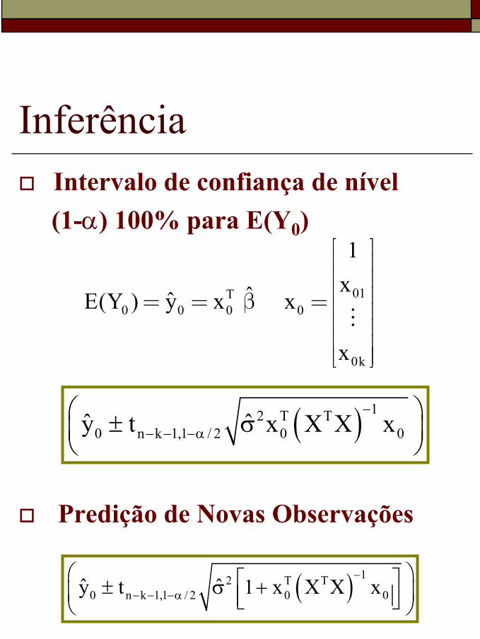
InferênciaIntervalo de confiança de nível (1-α) 100% para E(Y0)

Predição de Novas Observações

( ) 12 T T0 n k 1,1 / 2 0 0ˆ ˆy t x X X x

−

− − −α ± σ

01T0 0 0 0

0k

1xˆˆE(Y ) y x x

x

= = β =

( ) 12 T T0 n k 1,1 / 2 0 0ˆ ˆy t 1 x X X x

−

− − −α ± σ +

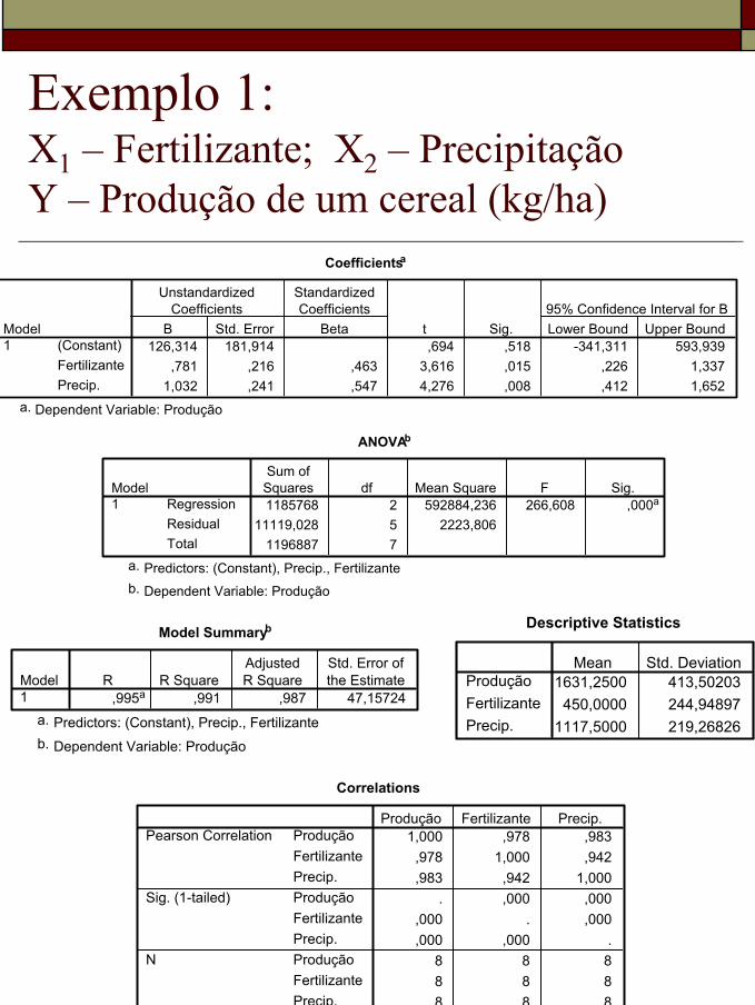
Exemplo 1:X1 – Fertilizante; X2 – Precipitação Y – Produção de um cereal (kg/ha)

Coefficientsa

126,314 181,914 ,694 ,518 -341,311 593,939,781 ,216 ,463 3,616 ,015 ,226 1,337

1,032 ,241 ,547 4,276 ,008 ,412 1,652

(Constant)FertilizantePrecip.

Model1

B Std. Error

UnstandardizedCoefficients

Beta

StandardizedCoefficients

t Sig. Lower Bound Upper Bound95% Confidence Interval for B

Dependent Variable: Produçãoa.

ANOVAb

1185768 2 592884,236 266,608 ,000a

11119,028 5 2223,8061196887 7

RegressionResidualTotal

Model1

Sum ofSquares df Mean Square F Sig.

Predictors: (Constant), Precip., Fertilizantea.

Dependent Variable: Produçãob.

Model Summaryb

,995a ,991 ,987 47,15724Model1

R R SquareAdjustedR Square

Std. Error ofthe Estimate

Predictors: (Constant), Precip., Fertilizantea.

Dependent Variable: Produçãob.

Correlations

1,000 ,978 ,983,978 1,000 ,942,983 ,942 1,000

. ,000 ,000,000 . ,000,000 ,000 .

8 8 88 8 88 8 8

ProduçãoFertilizantePrecip.ProduçãoFertilizantePrecip.ProduçãoFertilizantePrecip.

Pearson Correlation

Sig. (1-tailed)

N

Produção Fertilizante Precip.

Descriptive Statistics

1631,2500 413,50203450,0000 244,94897

1117,5000 219,26826

ProduçãoFertilizantePrecip.

Mean Std. Deviation

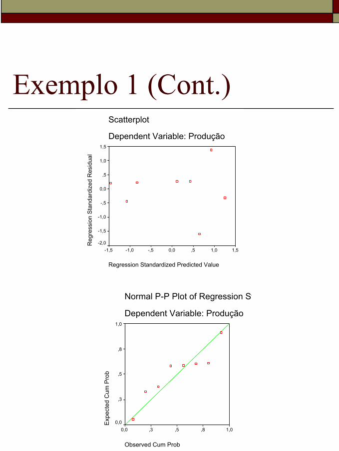
Exemplo 1 (Cont.)Scatterplot

Dependent Variable: Produção

Regression Standardized Predicted Value

1,51,0,50,0-,5-1,0-1,5

Reg

ress

ion

Sta

ndar

dize

d R

esid

ual

1,5

1,0

,5

0,0

-,5

-1,0

-1,5

-2,0

Normal P-P Plot of Regression St

Dependent Variable: Produção

Observed Cum Prob

1,0,8,5,30,0

Exp

ecte

d C

um P

rob

1,0

,8

,5

,3

0,0

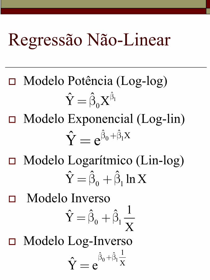
Regressão Não-Linear

Modelo Potência (Log-log)

Modelo Exponencial (Log-lin)

Modelo Logarítmico (Lin-log)

Modelo Inverso

Modelo Log-Inverso

1ˆ

0ˆY Xβ= β

0 1ˆ ˆ XY eβ +β=

0 1ˆ ˆY ln X= β +β

0 11ˆ ˆYX

= β + β

0 11ˆ ˆXY e

β +β=