RECTIFIABILITY AND ELLIPTIC MEASURES ON 1 …badger/ABHM_final.pdf · rectifiability and elliptic...
33
RECTIFIABILITY AND ELLIPTIC MEASURES ON 1-SIDED NTA DOMAINS WITH AHLFORS-DAVID REGULAR BOUNDARIES MURAT AKMAN, MATTHEW BADGER, STEVE HOFMANN, AND JOS ´ E MAR ´ IA MARTELL Abstract . Let Ω ⊂ R n+1 , n ≥ 2, be 1-sided NTA domain (aka uniform domain), i.e. a domain which satisfies interior Corkscrew and Harnack Chain conditions, and assume that ∂Ω is n-dimensional Ahlfors-David regular. We characterize the rectifiability of ∂Ω in terms of the absolute continuity of surface measure with respect to harmonic measure. We also show that these are equivalent to the fact that ∂Ω can be covered H n -a.e. by a countable union of portions of boundaries of bounded chord-arc subdomains of Ω and to the fact that ∂Ω possesses exterior corkscrew points in a qualitative way H n -a.e. Our methods apply to harmonic measure and also to elliptic measures associated with real symmetric second order divergence form elliptic operators with locally Lipschitz coefficients whose derivatives satisfy a natural qualitative Carleson condition. Contents 1. Introduction and statement of main results 2 1.1. Notation and conventions 5 1.2. Some definitions 6 1.3. Dyadic grids and sawtooths 7 2. Proof of Theorem 1.2 10 2.1. Proof of (a) implies (b) 10 2.2. Proof of (b) implies (d) 13 2.3. Proof of (d) implies (c) 15 2.4. Proof of (c) implies (d) 15 2.5. Proof of (b) implies (e) 24 3. Proof of Theorem 1.3 26 3.1. Proof of (c’) implies (d) 26 Date: July 6, 2015. 2010 Mathematics Subject Classification. 28A75, 28A78, 31A15, 31B05, 35J25, 42B37, 49Q15. Key words and phrases. NTA domains, 1-sided NTA domains, uniform domains, Ahlfors-David regular sets, rectifiability, harmonic measure, elliptic measure, surface measure, linearly approxima- bility, elliptic operators. The first and last authors have been supported in part by ICMAT Severo Ochoa project SEV- 2011-0087 and they acknowledge that the research leading to these results has received funding from the European Research Council under the European Union’s Seventh Framework Programme (FP7/2007-2013)/ ERC agreement no. 615112 HAPDEGMT. The second author was partially sup- ported by an NSF postdoctoral fellowship, DMS 1203497, and by NSF grant DMS 1500382. The third author was partially supported by NSF grant DMS 1361701. 1
Transcript of RECTIFIABILITY AND ELLIPTIC MEASURES ON 1 …badger/ABHM_final.pdf · rectifiability and elliptic...
RECTIFIABILITY AND ELLIPTIC MEASURES ON 1-SIDED NTADOMAINS WITH AHLFORS-DAVID REGULAR BOUNDARIES
MURAT AKMAN, MATTHEW BADGER, STEVE HOFMANN, AND JOSE MARIA MARTELL
Abstract. Let Ω ⊂ Rn+1, n ≥ 2, be 1-sided NTA domain (aka uniform domain),i.e. a domain which satisfies interior Corkscrew and Harnack Chain conditions,and assume that ∂Ω is n-dimensional Ahlfors-David regular. We characterize therectifiability of ∂Ω in terms of the absolute continuity of surface measure withrespect to harmonic measure. We also show that these are equivalent to the factthat ∂Ω can be covered Hn-a.e. by a countable union of portions of boundariesof bounded chord-arc subdomains of Ω and to the fact that ∂Ω possesses exteriorcorkscrew points in a qualitative way Hn-a.e. Our methods apply to harmonicmeasure and also to elliptic measures associated with real symmetric secondorder divergence form elliptic operators with locally Lipschitz coefficients whosederivatives satisfy a natural qualitative Carleson condition.
Contents
1. Introduction and statement of main results 21.1. Notation and conventions 51.2. Some definitions 61.3. Dyadic grids and sawtooths 72. Proof of Theorem 1.2 102.1. Proof of (a) implies (b) 102.2. Proof of (b) implies (d) 132.3. Proof of (d) implies (c) 152.4. Proof of (c) implies (d) 152.5. Proof of (b) implies (e) 243. Proof of Theorem 1.3 263.1. Proof of (c’) implies (d) 26
Date: July 6, 2015.2010 Mathematics Subject Classification. 28A75, 28A78, 31A15, 31B05, 35J25, 42B37, 49Q15.Key words and phrases. NTA domains, 1-sided NTA domains, uniform domains, Ahlfors-David
regular sets, rectifiability, harmonic measure, elliptic measure, surface measure, linearly approxima-bility, elliptic operators.
The first and last authors have been supported in part by ICMAT Severo Ochoa project SEV-2011-0087 and they acknowledge that the research leading to these results has received fundingfrom the European Research Council under the European Union’s Seventh Framework Programme(FP7/2007-2013)/ ERC agreement no. 615112 HAPDEGMT. The second author was partially sup-ported by an NSF postdoctoral fellowship, DMS 1203497, and by NSF grant DMS 1500382. Thethird author was partially supported by NSF grant DMS 1361701.
1
2 MURAT AKMAN, MATTHEW BADGER, STEVE HOFMANN, AND JOSE MARIA MARTELL
3.2. Proof of (b) implies (e’) 274. An example 28References 31
1. Introduction and statement of main results
A well known result of F. and M. Riesz says that if Ω is a simply connectedplanar domain whose boundary is a Jordan curve of finite length, then harmonicmeasure ω and arclength H1|∂Ω are mutually absolutely continuous. A quantita-tive version of this theorem was proved by Lavrentiev in [25]. Due to examplesof Bishop and Jones in [5] in the planar case, and of Ziemer in [33] and Wu in[32] in higher dimensions, neither Hn|∂Ω ω nor ω Hn are true for arbitrarysimply connected domains Ω ⊂ Rn+1 with Hn(∂Ω) < ∞ without imposing addi-tional topological and/or non-topological conditions on ∂Ω. Quantitative mutualabsolute continuity of harmonic measure and surface measure in higher dimen-sions was proven when Ω is a Lipschitz domain by Dahlberg in [9], and when Ω
is non-tangentially accessible (NTA) (see Definition 1.9) and ∂Ω is Ahlfors-Davidregular (ADR, see Definition 1.5) independently by David and Jerison in [11] andby Semmes in [31]. It is now known that if Ω is a 1-sided NTA domain (see Defi-nition 1.8) with ADR boundary, then the following are equivalent:
(i) ∂Ω is Uniformly Rectifiable,(ii) Ω is an NTA domain (and therefore Ω is a chord-arc domain),(iii) ω ∈ A∞,(iv) ω ∈ weak − A∞.
(1.1)
Here (iii) and (iv) should be understood in a scale invariant sense. The implication(i) implies (ii) was proved in [1]; (ii) implies (iii) was proved independently in[11, 31] as mentioned above; (iii) implies (iv) is trivial; and (iv) implies (i) wasproved in [21]. On the other hand, in [4], it was shown that if Ω is an NTA domainwithHn(∂Ω) < ∞, then ∂Ω is n-rectifiable andHn|∂Ω ω. Moreover, it was alsoshown in [4] that if Ω is an NTA domain, then ω Hn ω on A, where
A :=
x ∈ ∂Ω : lim infr→0
Hn(∂Ω ∩ B(x, r))rn < ∞
.
However, due to an example of Azzam, Mourgoglou, and Tolsa in [2], harmonicmeasure is not necessarily absolutely continuous with respect to surface measureon the entire boundary of an NTA domain of locally finite perimeter. In particular,the authors of [2] constructed Reifenberg flat domains Ω with locally finite surfacemeasureHn|∂Ω and Borel sets E ⊂ ∂Ω with ω(E) > 0 = Hn(E). (In fact, the sets Ehave Hausdorff dimension less than n.) Therefore, in order to ensure that ω Hn
on the full boundary of an NTA domain of locally finite perimeter, one needs toidentify some additional qualitative or quantitative conditions on ∂Ω. For relatedresults on p-harmonic measure, see [26].
The main result proved in this article is the following qualitative version of (1.1)(see Section 1.2 for the precise definitions).
RECTIFIABILITY AND ELLIPTIC MEASURES 3
Theorem 1.2. Let Ω ⊂ Rn+1, n ≥ 2, be a 1-sided NTA domain whose boundary isADR. Write ω := ωX0 for the harmonic measure of Ω with pole at X0, any givenpoint in Ω, and write σ := Hn|∂Ω for surface measure on ∂Ω. Then the followingstatements are equivalent:
(a) ∂Ω is rectifiable;(b) there exists a set F ⊂ ∂Ω and a constant c0, 0 < c0 < 1 such that σ(F) = 0
and for all x ∈ ∂Ω \ F there is rx > 0 for which ∆(x, r) = ∂Ω ∩ B(x, r) hasan exterior corkscrew point (that is, a corkscrew point with respect to theopen set Ωext = Rn+1 \Ω) for all 0 < r < rx with implicit constant c0;
(c) σ ω on ∂Ω;(d) ∂Ω = F0 ∪
(⋃N FN
), where σ(F0) = 0 and FN = ∂Ω ∩ ∂ΩN for some
bounded chord-arc domain ΩN ⊂ Ω;(e) ∂Ω = F0∪
(⋃N FN
), where σ(F0) = 0 and for each N there exist constants
θN , θ′N > 0 and CN > 1 such that
C−1N σ(F)θ
′N ≤ ω(F) ≤ CN σ(F)θN ∀ F ⊂ FN .
The proof of Theorem 1.2 is in Section 2 and goes as follows. First, observethat (e) easily gives (c). Second, (d) yields (a), because the boundary of any chordarc domain is rectifiable (e.g., see [11] or [4]). In Section 2.1, we use a notionof approximate tangent planes from geometric measure theory to show that (a)implies (b). Next, we prove in Section 2.2 that (b) implies (d) by constructingcertain sawtooth domains ΩF ,Q0 , which are bounded chord-arc subdomains of Ω.In Section 2.3, we verify (d) implies (c) by a straightforward use of the maximumprinciple. In Section 2.4, we first show that some family of bad cubes (for whichthe exterior corkscrew condition fails) satisfies a Carleson packing condition. Fromthere, we obtain that another suitable family of sawtooth domains ΩF ,Q0 are chord-arc domains and show that (c) implies (d). To complete the proof, in Section 2.5 wedemonstrate that (b) implies (e) by using a variant of the Dahlberg-Jerison-Kenigsawtooth lemma and a certain projection operator.
Although our main result is written in terms of harmonic measure, our methodsallow for more general elliptic measures. In particular, in Theorem 1.2 we canreplace harmonic measure ω with elliptic measures ωL corresponding to a class ofdivergence form elliptic operators whose coefficients are locally Lipschitz and obeya natural Carleson measure condition. Our class of operators is motivated by theresults in [24] and the recent work [19]. The operators considered in [24] have theproperty that they are good (i.e. their elliptic measure is A∞) in NTA subdomains.This is relevant in the proof of (b) implies (e), where such a property is used for theLaplacian. On the other hand, [19] contains a generalized version of the implication(iv) =⇒ (ii) in (1.1), valid for a class of elliptic operators. In [19], there is an“integration by parts” argument that allows the authors to obtain localized squarefunctions estimates and we use a similar argument here in the proof of (c) implies(d). Here we shall assume qualitative versions of the conditions in [24], [19] thatallow us to follow their ideas in a qualitative way. The precise result is as follows:
Theorem 1.3. Let Ω ⊂ Rn+1, n ≥ 2, be a 1-sided NTA domain whose bound-ary is ADR. Let Lu := − div(A∇u) and assume that A is uniformly elliptic, real,
4 MURAT AKMAN, MATTHEW BADGER, STEVE HOFMANN, AND JOSE MARIA MARTELL
symmetric, A ∈ Liploc(Ω), and for every ball B = B(x,R) with x ∈ ∂Ω and0 < R < diam(∂Ω), there exists CB such that
(1.4) supy∈B∩∂Ω0<r≤R
1rn
"B(y,r)∩Ω
(sup
Z∈B(X,δ(X)/2)|∇A(Z)|
)dX ≤ CB,
where δ(X) = dist(X, ∂Ω). Write ωL := ωX0L for the elliptic measure of Ω associated
to L with pole at X0, any given point in Ω, and write σ := Hn|∂Ω for surfacemeasure on ∂Ω. Then the equivalent statements (a)–(e) in Theorem 1.2 are alsoequivalent to the following statements:
(c’) σ ωL on ∂Ω;(e’) ∂Ω = F0∪
(⋃N FN
), where σ(F0) = 0 and for each N there exist constants
θN , θ′N > 0 and CN > 1 such that
C−1N σ(F)θ
′N ≤ ωL(F) ≤ CN σ(F)θN ∀ F ⊂ FN .
By an easy compactness argument, to invoke Theorem 1.3 it is enough to verifythat (1.4) holds on balls B = B(x,Rx) for every x ∈ ∂Ω, for some Rx > 0 dependingon x. Examples of operators Lu := − div(A∇u) where this result applies include thecase of coefficients A which are locally Lipschitz in Ω, with |∇A| ∈ L∞(B(x, rx)∩Ω)for every x ∈ ∂Ω, for some rx > 0. More generally, one may assume that there isε > 0 such that |∇A(X)| δ(X)1−ε → 0 as X → x along X ∈ Ω for every x ∈ ∂Ω.
The proof of Theorem 1.3 is given in Section 3. Note that (e’) easily implies(c’). To complete the proof, we show that (c’) implies (d) in Section 3.1 and (b)implies (e’) in Section 3.2.
Finally, in Section 4, we construct an example of a domain Ω? satisfying therequired background hypotheses (i.e. 1-sided NTA with ADR boundary) for which(a)–(e) in Theorem 1.2 hold, but (i)–(iv) in (1.1) fail. In particular, for this example,harmonic measure (and the elliptic measures in Theorem 1.3) belongs to neitherA∞ nor to weak-A∞, but nevertheless satisfies the weaker absolutely continuityconditions (c), (e) (and (c’), (e’)).
We note that some interesting related work has recently appeared, or been car-ried out, while this manuscript was in preparation, due to Mourgoglou [28], Azzam,Mourgoglou and Tolsa [3], and Mayboroda, Tolsa, Volberg and the two last authorsof the present paper [18] which sharpens our results in the special case of Laplace’sequation. In the first manuscript, the author obtains the implication (a) implies (c)of our Theorem 1.2, but with the upper ADR bound on ∂Ω replaced by the weakerqualitative condition that Hn|∂Ω is locally finite. Moreover, in [3], the authorsobtain the converse direction (c) implies (a) (as well as results concerning rectifia-bility of harmonic measure, provided that ω σ), replacing the ADR hypothesisby the weaker qualitative assumption that Hn|∂Ω is positive and locally finite, andassuming only a “porosity” (i.e. Corkscrew) condition in the complement of ∂Ω,in lieu of the stronger 1-sided NTA assumption. In [18] the same result is provedremoving the porosity assumption. Both [3] and the follow-up version [18] relyon recent deep results of [29], [30], concerning connections between rectifiabilityand the behavior of Riesz transforms. The use of these Riesz transform resultsallows for non-trivial weakening of the hypotheses as described above, but on the
RECTIFIABILITY AND ELLIPTIC MEASURES 5
other hand, the Riesz transforms are tied explicitly to harmonicity. Our methodsin the present paper, involving localized square function estimates, seem to requirea stronger connectivity hypothesis (i.e. the 1-sided NTA, aka “uniform domain”,assumption), but are more robust in the sense that they allow treatment of variablecoefficient operators.
A related result has been also obtained by the last two authors of the present pa-per in [17]: if Ω is an open set with ADR boundary and harmonic measure satisfiesa weak A∞ condition on ∂Ω then ∂Ω is Uniformly Rectifiable. This corresponds toa quantitative version of the implication (c) implies (a) of our Theorem 1.2 in a set-ting without connectivity assumptions. This result and the corresponding versionfor the p-Laplacian will appear in a forthcoming paper by the same two authors incollaboration with Le and Nystrom [15]. The converse of this result, that is, thatthe complement of a Uniformly Rectifiable set has “interior big pieces of good har-monic measure estimates”, has been recently proved by Bortz and the third authorof this paper [6]. This can be seen as a quantitative version of (c) (or (e)) implies(a) in Theorem 1.2.
1.1. Notation and conventions.
• We use the letters c,C to denote harmless positive constants, not necessarily thesame at each occurrence, which depend on at most dimension and the constantsappearing in the hypotheses of the theorems (that is, on “allowable parameters”).Unless otherwise specified, upper case constants are greater than 1 and lowercase constants are smaller than 1. We write a . b or a ≈ b to denote a ≤ Cb or0 < c ≤ a/b ≤ C for some constants c and C following the convention above,respectively.
• Given a domain Ω ⊂ Rn+1, we shall use lower case letters x, y, z, etc. to denotepoints on ∂Ω, and capital letters X,Y,Z, etc. to denote generic points in Rn+1
(especially those in Rn+1 \ ∂Ω).
• The open (n + 1)-dimensional Euclidean ball of radius r will be denoted B(x, r)when the center x lies on ∂Ω, and denoted B(X, r) when the center X ∈ Rn+1\∂Ω.A surface ball is denoted ∆(x, r) := B(x, r) ∩ ∂Ω.
• If ∂Ω is bounded, it is always understood (unless otherwise specified) that allsurface balls have radii controlled by the diameter of ∂Ω: that is, if ∆ = ∆(x, r),then r . diam(∂Ω). Note that in this way ∆ = ∂Ω if diam(∂Ω) < r . diam(∂Ω).
• Let dist(A, B) := infa∈A infb∈B |a−b| denote the usual Euclidean distance betweensets A and B. For X ∈ Rn+1, let δ(X) := dist(X, ∂Ω).
• LetHn denote n-dimensional Hausdorff measure and let σ := Hn∣∣∂Ω
denote thesurface measure on ∂Ω.
• For a generic set A ⊂ Rn+1, we let int(A) denote the interior of A. However,when A ⊂ ∂Ω, we let int(A) denote the interior of A relative to ∂Ω; that is, int(A)is the largest relatively open set in ∂Ω contained in A. In addition, for A ⊂ ∂Ω,we define the boundary ∂A := A \ int(A) using our convention on int(A).
6 MURAT AKMAN, MATTHEW BADGER, STEVE HOFMANN, AND JOSE MARIA MARTELL
• We shall use the letter I (and sometimes J) to denote a closed (n+1)-dimensionalEuclidean cube with sides parallel to the co-ordinate axes, and we let `(I) denotethe side length of I.
• We use Q to denote a dyadic “cube” on ∂Ω, which exists whenever ∂Ω is ADR(see [8, 13]) and enjoy certain properties enumerated in Lemma 1.13 below.
1.2. Some definitions.
Definition 1.5 (Ahlfors-David regular). We say that a closed set E ⊂ Rn+1 isn-dimensional ADR (or simply ADR) if there is some uniform constant C suchthat
1C
rn ≤ Hn(E ∩ B(x, r)) ≤ C rn ∀ r ∈ (0, diam(E)), x ∈ E.
Following [23], we state the definition of Corkscrew condition, Harnack Chaincondition, and NTA domains.
Definition 1.6 (Corkscrew condition). We say that an open set Ω ⊂ Rn+1 satisfiesthe (interior) Corkscrew condition if for some uniform constant c, 0 < c < 1, andfor every surface ball ∆ := ∆(x, r), with x ∈ ∂Ω and 0 < r < diam(∂Ω), there is aball B(X∆, cr) ⊂ B(x, r)∩Ω. The point X∆ ⊂ Ω is called a corkscrew point relativeto ∆, (or, relative to B). We note that we may allow r < C diam(∂Ω) for any fixedC, simply by adjusting the constant c.
Definition 1.7 (Harnack Chain condition). We say that Ω satisfies the HarnackChain condition if there is a uniform constant C such that for every ρ > 0, Λ ≥ 1,and every pair of points X, X′ ∈ Ω with δ(X), δ(X′) ≥ ρ and |X − X′| < Λ ρ, thereis a chain of open balls B1, . . . , BN ⊂ Ω, N ≤ C(Λ), with X ∈ B1, X′ ∈ BN ,Bk ∩ Bk+1 , Ø and C−1 diam(Bk) ≤ dist(Bk, ∂Ω) ≤ C diam(Bk). The chain of ballsis called a Harnack Chain.
Definition 1.8 (1-sided NTA domain). If Ω satisfies both the Corkscrew and Har-nack Chain conditions, then we say that Ω is a 1-sided NTA domain.
Definition 1.9 (NTA domain). We say that a domain Ω is an NTA domain if itis a 1-sided NTA domain and if, in addition, Ωext := Rn+1 \ Ω also satisfies theCorkscrew condition.
Remark 1.10. The abbreviation NTA stands for non-tangentially accessible. In theliterature, 1-sided NTA domains are also called uniform domains. We remark thatthe 1-sided NTA condition is a quantitative form of path connectedness.
Definition 1.11 (Chord-arc domain). A chord-arc domain Ω is an NTA domainwith ADR boundary.
We next give definition of rectifiability. For general background, see [27].
Definition 1.12 (Rectifiability). A set in E ⊂ Rn+1 is called n-rectifiable if thereexist Lipschitz maps fi : Rn → Rn+1, i = 1, 2, . . . , such that
Hn
(E \
∞⋃i=1
fi(Rn)
)= 0.
RECTIFIABILITY AND ELLIPTIC MEASURES 7
1.3. Dyadic grids and sawtooths. In this subsection we give a lemma concerningthe existence of “dyadic grid” which can be found in [13, 12, 8].
Lemma 1.13 (Existence and properties of the “dyadic grid”). If E ⊂ Rn+1 isADR, then there exist constants a0 > 0, η > 0, and C1 < ∞, depending only ondimension and the ADR constant, and for each k ∈ Z there exists a collection ofBorel sets (“cubes”)
Dk := Qkj ⊂ E : j ∈ Ik,
where Ik denotes some (possibly finite) index set depending on k, satisfying thefollowing properties.
(i) E =⋃
j Qkj for each k ∈ Z.
(ii) If m ≥ k then either Qmi ⊂ Qk
j or Qmi ∩ Qk
j = Ø.
(iii) For each ( j, k) and each m < k, there is a unique i such that Qkj ⊂ Qm
i .
(iv) The diameter of each Qkj is at most C12−k.
(v) Each Qkj contains some surface ball ∆
(xk
j, a02−k)
:= B(
xkj, a02−k
)∩ E.
(vi) Hn(
x ∈ Qkj : dist(x, E \ Qk
j) ≤ τ 2−k)≤ C1 τ
ηHn(
Qkj
)for all k and j
and for all τ ∈ (0, a0).
Some notations and remarks are in order concerning this lemma.
• In the setting of a general space of homogeneous type, this lemma has beenproved by Christ [8], with the dyadic parameter 1/2 replaced by some constantδ ∈ (0, 1). In fact, one may always take δ = 1/2 (cf. [22, Proof of Proposition2.12]). In the presence of ADR property, the result already appears in [12, 13].
• For our purposes, we may ignore those k ∈ Z such that 2−k & diam(E) wheneverE is bounded.
• We shall denote by D = D(E) the collection of all relevant Qkj. That is,
D :=⋃
k
Dk,
where the union runs only over those k such that 2−k . diam(E) whenever E isbounded.
• Given a cube Q ∈ D, we set
DQ :=
Q′ ∈ D : Q′ ⊆ Q.
• For a dyadic cube Q ∈ Dk, we set `(Q) = 2−k and we call this quantity the“length” of Q. Evidently, `(Q) ≈ diam(Q).
• Properties (iv) and (v) imply that for each cube Q ∈ Dk, there exists a pointxQ ∈ E, a Euclidean ball B(xQ, rQ) and corresponding surface ball ∆(xQ, rQ) :=B(xQ, rQ) ∩ E such that
(1.14) c`(Q) ≤ rQ ≤ `(Q) and ∆(xQ, 2rQ) ⊂ Q ⊂ ∆(xQ,CrQ)
8 MURAT AKMAN, MATTHEW BADGER, STEVE HOFMANN, AND JOSE MARIA MARTELL
for some uniform constants c and C. We shall denote this ball and surface ballby BQ := B(xQ, rQ) and ∆Q := ∆(xQ, rQ), respectively, and we shall refer to thepoint xQ as the “center” of Q.
It will be useful to dyadicize the Corkscrew condition and to specify preciseCorkscrew constants. Let us now specialize to the case that E = ∂Ω is ADR withΩ satisfying the Corkscrew condition. Given Q ∈ D(∂Ω), we shall sometimes referto a corkscrew point XQ relative to Q, which define to be a corkscrew point X∆
relative to the surface ball ∆ := ∆Q We note that δ(XQ) ≈ dist(XQ,Q) ≈ diam(Q).
Definition 1.15 (c0-exterior Corkscrew condition). Fix a constant c0 ∈ (0, 1) andlet Ω ⊂ Rn+1 be a domain with ADR boundary. We say that a cube Q ∈ D(∂Ω)satisfies the the c0-exterior Corkscrew condition if there is a point zQ ∈ ∆Q anda point X−Q ∈ B(zQ, rQ/4) \ Ω such that B(X−Q, c0 `(Q)) ⊂ B(zQ, rQ/4) \ Ω, where∆Q = ∆(xQ, rQ) is the surface ball associated to Q.
Following [16, Section 3] we next introduce the notion of Carleson region anddiscretized sawtooth. Given a cube Q ∈ D(∂Ω), the discretized Carleson regionDQ relative to Q is defined by
DQ = Q′ ∈ D(∂Ω) : Q′ ⊂ Q.
Let F be family of disjoint cubes Q j ⊂ D(∂Ω). The global discretized sawtoothregion relative to F is the collection of cubes Q ∈ D that are not contained in anyQ j ∈ F ;
DF := D \⋃
Q j∈F
DQ j .
For a given Q ∈ D the local discretized sawtooth region relative to F is thecollection of cubes in DQ that are not in contained in any Q j ∈ F ;
DF ,Q := DQ \⋃
Q j∈F
DQ j = DF ∩ DQ.
We also introduce the “geometric” Carleson regions and sawtooths. In the sequel,Ω ⊂ Rn+1 (n ≥ 2) will be a 1-sided NTA domain with ADR boundary. LetW =
W(Ω) denote a collection of (closed) dyadic Whitney cubes of Ω, so that the cubesinW form a covering of Ω with non-overlapping interiors, and which satisfy
(1.16) 4 diam (I) ≤ dist(4I, ∂Ω) ≤ dist(I, ∂Ω) ≤ 40 diam (I)
and
(1.17) diam(I1) ≈ diam(I2), whenever I1 and I2 touch.
Let X(I) denote the center of I, let `(I) denote the side length of I, and write k = kIif `(I) = 2−k.
Given 0 < λ < 1 and I ∈ W we write I∗ = (1 + λ)I for the “fattening” of I. Bytaking λ small enough, we can arrange matters so that, first, dist(I∗, J∗) ≈ dist(I, J)for every I, J ∈ W, and secondly, I∗ meets J∗ if and only if ∂I meets ∂J. (Fatteningensures I∗ and J∗ overlap for any pair I, J ∈ W whose boundaries touch. Thus, theHarnack Chain property holds locally in I∗ ∪ J∗ with constants depending on λ.)By picking λ sufficiently small, say 0 < λ < λ0, we may also suppose that there is
RECTIFIABILITY AND ELLIPTIC MEASURES 9
τ ∈ (1/2, 1) such that for distinct I, J ∈ W, τJ ∩ I∗ = Ø. In what follows we willneed to work with dilations I∗∗ = (1 + 2 λ)I and in order to ensure that the sameproperties hold we further assume that 0 < λ < λ0/2.
For every Q we can construct a familyW∗Q ⊂ W and define
(1.18) UQ :=⋃
I∈W∗Q
I∗ ,
satisfying the following properties: XQ ∈ UQ and there are uniform constants k∗
and K0 such that
k(Q) − k∗ ≤ kI ≤ k(Q) + k∗ ∀ I ∈ W∗Q,(1.19)
X(I)→UQ XQ ∀ I ∈ W∗Q,
dist(I,Q) ≤ K0 2−k(Q) ∀ I ∈ W∗Q .
Here X(I)→UQ XQ means that the interior of UQ contains all the balls in a HarnackChain (in Ω) connecting X(I) to XQ, and moreover, for any point Z contained inany ball in the Harnack Chain, we have dist(Z, ∂Ω) ≈ dist(Z,Ω \UQ) with uniformcontrol of the implicit constants. The constants k∗, K0 and the implicit constants inthe condition X(I) →UQ XQ in (1.19) depend on at most allowable parameters andon λ. The reader is referred to [16] for full details.
For a given Q ∈ D, the Carleson box relative to Q is defined by
TQ := int
⋃Q′∈DQ
UQ′
.
For a given family F of disjoint cubes Q j ⊂ D, the global sawtooth regionrelative to F is
ΩF := int
⋃Q′∈DF
UQ′
.
Finally, for a given Q ∈ D we define the local sawtooth region relative to F by
ΩF ,Q := int
⋃Q′∈DF ,Q
UQ′
.
For later use we recall [16, Proposition 6.1]:
Q \( ⋃
Q j∈F
Q j
)⊂ ∂Ω ∩ ∂ΩF ,Q ⊂ Q \
( ⋃Q j∈F
int(Q j)).(1.20)
Given a pairwise disjoint family F ∈ D and a constant ρ > 0, we derive anotherfamily F (ρ) ⊂ D from F as follows. Augment F by adding cubes Q ∈ D whoseside length `(Q) ≤ ρ and let F (ρ) denote the corresponding collection of maximalcubes. Note that the corresponding discrete sawtooth region DF (ρ) is the union ofall cubes Q ∈ DF such that `(Q) > ρ. For a given constant ρ and a cube Q ∈ D,let DF (ρ),Q denote the local discrete sawtooth region and let ΩF (ρ),Q denote thegeometric sawtooth region relative to disjoint family F (ρ).
10 MURAT AKMAN, MATTHEW BADGER, STEVE HOFMANN, AND JOSE MARIA MARTELL
2. Proof of Theorem 1.2
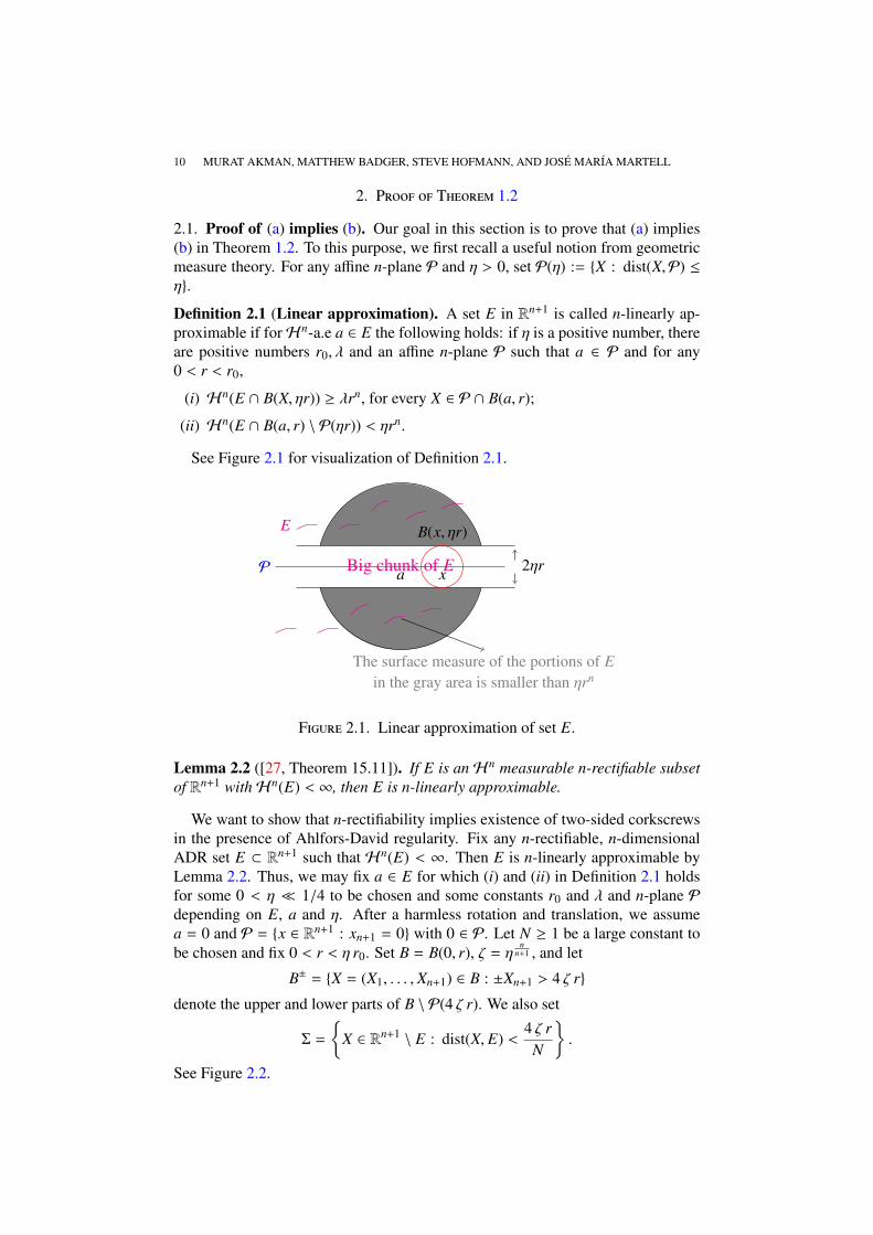
2.1. Proof of (a) implies (b). Our goal in this section is to prove that (a) implies(b) in Theorem 1.2. To this purpose, we first recall a useful notion from geometricmeasure theory. For any affine n-plane P and η > 0, set P(η) := X : dist(X,P) ≤η.
Definition 2.1 (Linear approximation). A set E in Rn+1 is called n-linearly ap-proximable if forHn-a.e a ∈ E the following holds: if η is a positive number, thereare positive numbers r0, λ and an affine n-plane P such that a ∈ P and for any0 < r < r0,
(i) Hn(E ∩ B(X, ηr)) ≥ λrn, for every X ∈ P ∩ B(a, r);
(ii) Hn(E ∩ B(a, r) \ P(ηr)) < ηrn.
See Figure 2.1 for visualization of Definition 2.1.
B(x, ηr)
The surface measure of the portions of Ein the gray area is smaller than ηrn
E
P xa 2ηrBig chunk of E
Figure 2.1. Linear approximation of set E.
Lemma 2.2 ([27, Theorem 15.11]). If E is anHn measurable n-rectifiable subsetof Rn+1 withHn(E) < ∞, then E is n-linearly approximable.
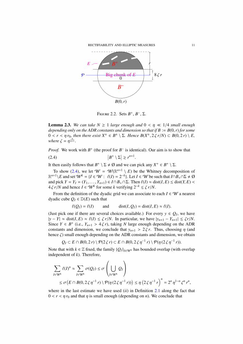
We want to show that n-rectifiability implies existence of two-sided corkscrewsin the presence of Ahlfors-David regularity. Fix any n-rectifiable, n-dimensionalADR set E ⊂ Rn+1 such that Hn(E) < ∞. Then E is n-linearly approximable byLemma 2.2. Thus, we may fix a ∈ E for which (i) and (ii) in Definition 2.1 holdsfor some 0 < η 1/4 to be chosen and some constants r0 and λ and n-plane Pdepending on E, a and η. After a harmless rotation and translation, we assumea = 0 and P = x ∈ Rn+1 : xn+1 = 0 with 0 ∈ P. Let N ≥ 1 be a large constant tobe chosen and fix 0 < r < η r0. Set B = B(0, r), ζ = η
nn+1 , and let
B± = X = (X1, . . . , Xn+1) ∈ B : ±Xn+1 > 4 ζ r
denote the upper and lower parts of B \ P(4 ζ r). We also set
Σ =
X ∈ Rn+1 \ E : dist(X, E) <
4 ζ rN
.
See Figure 2.2.
RECTIFIABILITY AND ELLIPTIC MEASURES 11
B(0, r)
E
P 8 ζ r
B+ r
0
B−
Big chunk of E
Figure 2.2. Sets B+, B−, Σ.
Lemma 2.3. We can take N ≥ 1 large enough and 0 < η 1/4 small enoughdepending only on the ADR constants and dimension so that if B := B(0, r) for some0 < r < η r0, then there exist X± ∈ B± \ Σ. Hence B(X±, 2 ζ r/N) ⊂ B(0, 2 r) \ E,where ζ = η
nn+1 .
Proof. We work with B+ (the proof for B− is identical). Our aim is to show that∣∣B+ \ Σ∣∣ & rn+1.(2.4)
It then easily follows that B+ \ Σ , Ø and we can pick any X+ ∈ B+ \ Σ.To show (2.4), we let W = W(Rn+1 \ E) be the Whitney decomposition of
Rn+1\E and setWk = I ∈ W : `(I) = 2−k. Let I ∈ W be such that I∩B+∩Σ , Øand pick Y = YI = (Y1, . . . ,Yn+1) ∈ I∩B+∩Σ. Then `(I) ≈ dist(I, E) ≤ dist(Y, E) <4 ζ r/N and hence I ∈ Wk for some k verifying 2−k . ζ r/N.
From the definition of the dyadic grid we can associate to each I ∈ W a nearestdyadic cube QI ∈ D(E) such that
`(QI) = `(I) and dist(I,QI) = dist(I, E) ≈ `(I).
(Just pick one if there are several choices available.) For every y ∈ QI , we have|y − Y | ≈ dist(I, E) ≈ `(I) . ζ r/N. In particular, we have |yn+1 − Yn+1| . ζr/N.Since Y ∈ B+ (i.e., Yn+1 > 4 ζ r), taking N large enough depending on the ADRconstants and dimension, we conclude that yn+1 > 2 ζ r. Thus, choosing η (andhence ζ) small enough depending on the ADR constants and dimension, we obtain
QI ⊂ E ∩ B(0, 2 r) \ P(2 ζ r) ⊂ E ∩ B(0, 2 ζ η−1 r) \ P(η (2 ζ η−1 r)).
Note that with k ∈ Z fixed, the family QII∈Wk has bounded overlap (with overlapindependent of k). Therefore,
∑I∈Wk
`(I)n ≈∑
I∈Wk
σ(QI) . σ
⋃I∈Wk
QI
≤ σ
(E ∩ B(0, 2 ζ η−1 r) \ P(η (2 ζ η−1 r))
)≤ η(2 ζ η−1 r
)n= 2n η1−n ζn rn,
where in the last estimate we have used (ii) in Definition 2.1 along the fact that0 < r < η r0 and that η is small enough (depending on n). We conclude that
12 MURAT AKMAN, MATTHEW BADGER, STEVE HOFMANN, AND JOSE MARIA MARTELL
(2.5) |B+ ∩ Σ| =∑I∈W
|I ∩ B+ ∩ Σ| ≤∑
k: 2−k. ζ rN
∑I∈Wk
`(I)n+1
≤∑
k: 2−k. ζ rN
2−k∑
I∈Wk
`(I)n . η1−n ζn+1 rn+1 = η rn+1.
This and [16, Lemma 5.3] easily imply
rn+1 ≈∣∣B ∩ X ∈ Rn+1 : 0 < Xn+1 ≤ 4 ζ r
∣∣ + |B+ ∩ Σ| + |B+ \ Σ|
. (ζ + η) rn+1 + |B+ \ Σ|.
Taking now η > 0 small enough depending only on ADR constants and dimension,we can hide the first time in the last term and conclude as desired (2.4).
We are now ready to establish the main result of this section:
Proposition 2.6. Let Ω be a 1-sided NTA domain with ADR boundary and assumethat ∂Ω is n-rectifiable. There exists 0 < c < 1 depending on the 1-sided NTA andADR constants such that for σ-a.e. x ∈ ∂Ω there is a scale rx > 0 such that forall 0 < r < rx there exist Xint
∆(x,r), Xext∆(x,r) ∈ B(x, r) that are respectively interior and
exterior corkscrew points relative to ∆(x, r) with implicit constant c.
Proof. We first consider the case on which E = ∂Ω is bounded so that σ(∂Ω) < ∞.We can then use Lemma 2.2 to find a subset of ∂Ω with full σ-measure on which(i) and (ii) of Definition 2.1 hold. We can make the previous reductions and findX± as in Lemma 2.3 associated with B := B(0, r) whenever 0 < r < η r0, whereN ≥ 1 is a fixed small number and η is small enough but at our disposal.
We claim that if η is small enough depending on the 1-sided NTA and ADRconstants, then at least one of X± belongs to Ωext. Suppose otherwise that X± ∈ Ω
(by construction X± < ∂Ω). Since Ω is a 1-sided NTA domain, Ω is also a uniformdomain. In fact, the two notions are equivalent; see [1] for the definition of auniform domain and for a proof of the direction that is relevant here. Thus, thereexist 0 < c1 < 1 and C1 > 1 depending only the 1-sided NTA constants and a pathγ connecting X+ and X− in Ω so that
`(γ) ≤ C1 |X− − X+| and dist(Z, ∂Ω) ≥ c1 dist(Z, X−, X+) ∀Z ∈ γ.
In the previous expression, `(γ) denotes the length of γ. For every Y ∈ γ, we have
|Y | ≤ |Y − X+| + |X+| ≤ diam(γ) + r ≤ `(γ) + r ≤ C1 |X− − X+| + r ≤ (2 C1 + 1) r,
since X+ ∈ γ. Hence γ ⊂ B(0, (2 C1 + 1) r). On the other hand X± ∈ B±. HenceX+ lies above P and X− lies below P. In particular, we can thus find Z ∈ P ∩ γ ⊂P ∩ B(0, (2 C1 + 1) r). If we assume that (2 C1 + 1) r < r0, then we can apply (i) inDefinition 2.1 to find z ∈ ∂Ω such that dist(Z, ∂Ω) ≤ |Z − z| < η (2 C1 + 1) r. Alsonote that since Z ∈ P and X± ∈ B±,
|Z − X±| ≥ |X±n+1| > 4 ζ r = 4 ηn
n+1 r.
Hence
η (2 C1 + 1) r > dist(Z, ∂Ω) ≥ c1 dist(Z, X−, X+) ≥ c1 4 ηn
n+1 r.
RECTIFIABILITY AND ELLIPTIC MEASURES 13
We can clearly take η arbitrarily small depending only on C1, c1 and n so that theprevious estimate does not hold and this brings us to a contradiction.
Let us summarize the argument so far. We can pick η0 small enough (dependingon the 1-sided NTA and ADR constants) so that if
0 < r < rx := r0 minη0, (2 C1 + 1)−1,
then X+ or X− is in Ωext. Let Xext denote one of the points in Ωext. By Lemma 2.3,B(Xext, 2 ζ0 r/N)) ⊂ B(0, 2 r) \ ∂Ω and hence Xext is an exterior corkscrew pointrelative to ∆(0, 2 r) with implicit constant ζ0/N. On the other hand since Ω is a 1-sided NTA domain it satisfies the (interior) corkscrew condition and hence we canfind Xint an interior corkscrew point relative to ∆(0, 2 r) with implicit constant c0.This readily leads to the desired conclusion with rx as above and c = minζ0/N, c0.This completes the proof in the case that ∂Ω is compact.
Suppose that ∂Ω is unbounded and proceed as follows. Cover ∂Ω by the disjoint(countable) family of Q ∈ D with `(Q) = 1. Fix one of these cubes, say Q0. Werecall that Q0 ⊂ ∆∗Q0
:= ∆(xQ0 ,C rQ0). Consider the Carleson box Ω0 := T∆∗Q0(see [16, Section 3]). By [16, Lemma 3.61], Ω0 is a 1-sided NTA domain withADR boundary and the implicit constants are uniform and depend only on thosefor Ω and dimension. Also, Ω0 ⊂ B(xQ0 , κ0rQ0) for some large κ0. In particular,Ω0 is bounded and so is its boundary. Finally, observe that ∂Ω0 = (∂Ω0 ∩ ∂Ω) ∪(∂Ω0 ∩ Ω). The first portion is n-rectifiable since so is ∂Ω. From the construction,the second portion is a countable union of partial faces of Whitney boxes and isthus also n-rectifiable. Because ∂Ω0 is n-rectifiable and compact, the argumentabove implies existence of two-sided corkscrews Hn-almost everywhere on ∂Ω0.From [16, Section 3], we have that B∗Q0
∩ Ω ⊂ 54 B∗Q0
∩ Ω ⊂ Ω0. Hence for Hn-a.e. x ∈ ∆∗Q0
there is rx so that for every 0 < r < rx we can find Xext ∈ (Ω0)ext withB(Xext, c r) ⊂ B(x, r)∩ (Ω0)ext. Note that by assuming further that 0 < r < rQ0/100,we actually have B(Xext, c r) ⊂ Ωext as the distance from any point in ∆∗Q0
to Ωext∩Ω
is at least 14 rQ0 . Finally, since Ω is 1-sided NTA, we can find the interior corkscrew
relative to ∆(x, r). Hence we have two-sided corkscrews σ-a.e. in ∆∗Q0in the sense
described above. This can be done for every Q0 with `(Q0) = 1, which cover ∂Ω.This completes the proof in the case that ∂Ω is unbounded.
2.2. Proof of (b) implies (d). In this section, we prove (b) implies (d). Supposethere exist a Borel measurable set F0 ⊂ ∂Ω with σ(F0) = 0 and constant 0 < 2 c0 <1 such that:
For each x ∈ ∂Ω \ F0, there is a scale 0 < rx < diam(∂Ω) such thatfor every 0 < r < rx there exist interior and exterior corkscrewpoints relative to ∆(x, r) with implicit constant 2 c0.
By taking rx smaller if needed, we may assume that rx = 2−kx for some kx ∈ Z.Given k ∈ Z we consider the closed set (and therefore measurable set)
Ek := x ∈ ∂Ω \ F0 : rx = 2−k.
Then ∂Ω = F0 ∪⋃
k∈Z Ek. In turn, for each k we can write Ek =⋃
Q∈DkEk ∩ Q.
To establish (d), it suffices to show that for every k ∈ Z and Q ∈ Dk, there exists abounded-chord arc domain Ω? ⊂ Ω such that Ek ∩ Q ⊂ ∂Ω ∩ ∂Ω?.
14 MURAT AKMAN, MATTHEW BADGER, STEVE HOFMANN, AND JOSE MARIA MARTELL
Fix k ∈ Z and Q0 ∈ Dk for which Ek∩Q0 , Ø. Suppose x ∈ Ek and 0 < r < 2−k.Then there exists y ∈ ∂Ω \ F0 such that ry = 2−k and |x − y| < r/2. Let X± beinterior/exterior corkscrew points relative to ∆(y, r/2) with implicit constant 2c0and note that
B(X±, c0 r) = B(X±, 2 c0 (r/2)) ⊂ B(y, r/2) ∩Ω± ⊂ B(x, r) ∩Ω±,
where Ω+ and Ω− denote Ω and Ωext, respectively. We conclude that for every x ∈Ek and for every 0 < r < 2−k there are interior/exterior corkscrew points X± relativeto ∆(x, r) with implicit constant c0. This is the key property for the rest of theargument in this section. To continue, set Fk = Ek ∩ Q0 and dyadically subdivideQ0, stopping whenever Q ∩ Fk = Ø. If we never stop, set F = Ø. Otherwise,F = Q j j≥1 ⊂ DQ0 \ Q0 is the pairwise collection of stopping time dyadic cubesand it follows that Q j ∩ Fk = Ø and Q ∩ Fk , Ø whenever Q j ( Q ⊂ Q0. Weremark that we did not stop at Q0, because Fk , Ø. Also, Fk = Q0 \
⋃j≥1 Q j,
because Ek is a closed set.Set Ω? = ΩF ,Q0 (where it is understood that Ω? = TQ0 if F = Ø). Then Ω? is
a bounded 1-sided NTA domain with ADR boundary by [16, Lemma 3.61], whereall implicit constants for Ω? depend only on the corresponding constants for Ω. By(1.20), we only need to check that Ω? satisfies the exterior corkscrew condition,which will follow from the definition of the set Fk.
To complete the proof, let M > 1 denote a large constant to be chosen below.Fix any boundary point x ∈ ∂Ω? and any scale 0 < r < 2−k = `(Q0) ≈ diam(∂Ω?),and set ∆? = B(x, r) ∩ ∂Ω?. We consider two cases:Case 1: Suppose that 0 ≤ δ(x) ≤ r/M, where δ(x) = dist(x, ∂Ω). We first claim thatthere exists Q ∈ DQ0 with `(Q) ≈ r/M such that |x − xQ| . r/M. To see this, notethat on one hand, if x ∈ ∂Ω?∩∂Ω, then x ∈ Q0 (see (1.20)) and we can find Q ∈ DQ0
with `(Q) ≈ r/M and x ∈ Q. On the other hand, if x ∈ ∂Ω? ∩ Ω, then by thedefinition of the sawtooth region, x ∈ ∂I∗ for some I ∈ W∗
Q′ with Q′ ∈ DF ,Q0 and|x − xQ′ | ≈ dist(I,Q′) ≈ `(Q′) ≈ `(I) ≈ δ(x) ≤ r/M. Let us now take Q ∈ DQ0 , anancestor of Q′, such that `(Q) ≈ r/M and hence |x−xQ| ≤ |x−xQ′ |+|xQ′−xQ| . r/M.This verifies the claim.
Take Q as in the claim and consider two cases. Suppose first that there existsy ∈ Q ∩ Fk , Ø. Then, as shown above, there is X− such that B(X−, c0 r/2) ⊂B(y, r/2) ∩Ωext. Therefore, for M large enough, we have
B(X−, c0 r/2) ⊂ B(y, r/2) ∩Ωext ⊂ B(x, r) ∩ (Ω?)ext.
Suppose otherwise that Q∩ Fk = Ø. Then Q ⊂⋃
j≥1 Q j, say Q∩ Qi , Ø for someQi ∈ F . Recall that Qi, the father of Qi, meets Fk and therefore Q ⊂ Qi. Thus,by [16, Lemma 5.9], there is a ball B′ ⊂ Rn+1 \ Ω? whose center is xQ and whoseradius is of the order of `(Q) ≈ r/M. For M large enough, this gives the desiredexterior corkscrew condition relative to ∆?. This completes Case 1.Case 2: Suppose that δ(x) > r/M. Then x ∈ Ω, and by definition of the sawtoothregion, x ∈ ∂I∗ ∩ J for some Whitney cubes I ∈ W∗
Q, Q ∈ DF ,Q0 , and J ∈ W withτ J ⊂ Ω \Ω? for some τ ∈ (1/2, 1). Note that `(I) ≈ `(J) ≈ δ(x) > r/M. Hence wecan easily find an exterior corkscrew in the segment joining x with the center of J
RECTIFIABILITY AND ELLIPTIC MEASURES 15
with corkscrew constant that depends only on M and the implicit constants in theprevious estimates. This completes Case 2.
This finishes the proof of (b) implies (d).
2.3. Proof of (d) implies (c). The argument is quite simple. Let F ⊂ ∂Ω be aBorel set and suppose thatω(F) = 0. Thenω(F∩FN) = 0 for every N and it sufficesto show that σ(F ∩ FN) = 0 for each N. Fix N and write ωN for the harmonicmeasure of ΩN with pole at XN , any point of ΩN . By Harnack’s inequality and themaximum principle (see the justification below), 0 ≤ ωN(F∩FN) ≤ ωXN (F∩FN) =
0. But ωN ∈ A∞(∂ΩN), since ΩN is a chord-arc domain (see [11, 31]). HenceωN and Hn
∣∣∂ΩN
are mutually absolutely continuous. Therefore, σ(F ∩ FN) = 0,because ωN(F ∩ FN) = 0.
Let us justify the use of maximum principle. One can use Perron’s method (see[14, Chapter 2] for more details) to easily see that every superfunction relative toχF∩FN for Ω is also a superfunction relative to χF∩FN for ΩN , since ΩN ⊂ Ω and F∩FN ⊂ ∂Ω∩∂ΩN . Hence the desired inequality follows after taking the infimum oversuch superfunctions. This works for the Laplacian and does not require Wienerregularity. However, since below we are also interested in the case of variablecoefficients, we now present a more robust, alternative argument, borrowed from[20]. Fix a compact set F ⊂ F ∩ FN and a small error ε > 0. Since ωXN is outerregular, there exists a bounded, relatively open set U ⊂ ∂Ω such that F ⊂ U and
ωXN (U) ≤ ωXN (F) + ε.
By Urysohn’s lemma there exists ϕ ∈ Cc(∂Ω) such that 0 ≤ ϕ ≤ 1, ϕ ≡ 1 on F andϕ ≡ 0 on ∂Ω \ U. Let u denote the Poisson extension of ϕ, i.e.,
u(X) :=∫∂Ω
ϕ(y) dωX(y) ∀ X ∈ Ω.
Because ∂Ω is ADR, every x ∈ ∂Ω is regular in the sense of Wiener (e.g. see [20]).Hence u ∈ C(Ω), where u|∂Ω = ϕ, and thus, u ∈ C(ΩN), as well. It follows that
(2.7) ωN(F) =
∫∂ΩN
1F(y) dωN(y) ≤∫∂ΩN
u(y) dωN(y) = u(XN),
where the last equality holds by the strong maximum principle and the fact that ΩNis bounded. On the other hand,
(2.8) u(XN) ≤∫∂Ω
χU(y) dωXN (y) = ωXN (U) ≤ ωXN (F) + ε.
Combining (2.7) and (2.8) and letting ε → 0, we conclude that ωN(F) ≤ ωXN (F)for every compact set F ⊂ F ∩ FN Therefore, since ωN and ωXN are inner regular,ωN(F ∩ FN) ≤ ωXN (F ∩ FN), as claimed above.
2.4. Proof of (c) implies (d). In this section we prove (c) implies (d). Assumethat σ ω. Fix Q0 ∈ Dk0 where k0 ∈ Z is taken so that 2−k0 diam(∂Ω). Fromthe construction of TQ0 one can easily see that TQ0 ⊂ κ0 BQ := B∗Q0
, where κ0 is aconstant depending on the ADR and 1-sided NTA constants and the parameters in(1.19) (see [16]). Let X0 be an interior corkscrew point for κ∆∗Q0
where κ is a large,but fixed constant, for which so that X0 < 4 B∗Q0
. Note that implicitly, we need
16 MURAT AKMAN, MATTHEW BADGER, STEVE HOFMANN, AND JOSE MARIA MARTELL
`(Q0) diam(∂Ω). Since ∂Ω is ADR, Bourgain’s alternative [7] and Harnack’sinequality gives ωX0(Q0) ≥ C−1
0 , where C0 ≥ 1 depends on ADR constants and κ.Thus, ω := C0 σ(Q0)ωX0 satisfies
1 ≤ω(Q0)σ(Q0)
≤ C0.(2.9)
Let N ≥ C0 and let FN = Q j ⊂ DQ0 \ Q0 be the collection of descendants of Q0that are maximal with respect to the property that either
ω(Q j)σ(Q j)
<1N
orω(Q j)σ(Q j)
> N.(2.10)
By maximality, it follows that
1N<ω(Q)σ(Q)
≤ N ∀Q ∈ DFN ,Q0 .(2.11)
On the other hand, we can write
(2.12) Q0 =
( ⋂N≥C0
⋃Q j∈FN
Q j
)∪
( ⋃N≥C0
(Q0 \
⋃Q j∈FN
Q j
))=: E0 ∪
( ⋃N≥C0
EN
).
The fact that σ ω implies
(2.13) σ(E0) ≤ σ(x ∈ Q0 : dσ/dω = 0 or dσ/dω = ∞
)= 0.
The following proposition is the core result of this section.
Proposition 2.14. ΩFN ,Q0 is chord-arc domain for every N ≥ C0.
Observe that EN = Q0\⋃
Q j∈FN
Q j ⊂ ∂Ω∩∂ΩFN ,Q0 (cf. (1.20)). This, (2.12), (2.13)
and the previous proposition give (d) for the portion of the boundary correspondingto Q0. Now we observe that ∂Ω =
⋃Q∈Dk0
Q and (d) follows.
The proof of Proposition 2.14 being somewhat long, we break the argument intoseveral steps. Fix any integer N ≥ C0. Let η(N) be a sufficiently small constantdepending on N to be specified below. Recalling Definition 1.15 we set
BN :=
Q ∈ DQ0 : Q does not satisfy the η(N)-exterior Corkscrew condition.
Let us introduce some additional notation. For every Q ∈ DQ0 , we set
(2.15) αQ :=
σ(Q) , if Q ∈ Q ∈ DFN ,Q0 ∩ B
N ,
0 , otherwise.
For any subcollection D′ ⊂ DQ0 , we set
(2.16) m(D′) :=∑Q∈D′
αQ.
We shall see that the family DFN ,Q0 ∩BN satisfies a packing condition with respect
to the surface measure provided that η(N) is small enough; that is, m is a discreteCarleson measure. In the argument that follows, we emphasize that constants areallowed to depend on N.
RECTIFIABILITY AND ELLIPTIC MEASURES 17
Lemma 2.17. Under the setup above, for each N ≥ C0 there exists 0 < CN < ∞(independent of Q0) such that if η(N) is small enough (depending on N and theADR and 1-sided NTA constants of Ω), then m is a discrete Carleson measure:
supQ′0∈DQ0
m(DQ′0)σ(Q′0)
= supQ′0∈DQ0
1σ(Q′0)
∑Q∈DQ′0
Q∈DFN ,Q0∩BN
σ(Q) ≤ CN < ∞.(2.18)
Proof. We first normalize the Green function G(X0, ·). Set
G(Y) := C−10 σ(Q0) G(X0,Y),
where X0 is the corkscrew point relative to κ∆∗Q0as explained above and C0 is the
constant as in (2.9). Note that our choice of X0 guarantees that G ∈ W1,20 (2 B∗Q0
∩Ω)and G is harmonic in 2 B∗Q0
∩ Ω. Because all of our estimates below take placein 2 B∗Q0
∩ Ω (since TQ0 ⊂ B∗Q0∩ Ω), this observation ensures the computations
below are meaningful. Also, use of a Caffarelli-Fabes-Mortola-Salsa estimate anddoubling of ω in 2 ∆∗Q0
are legitimate under this regime; for this and more in thesetting of 1-sided NTA domains, see [20].
Fix a cube Q ∈ DFN ,Q0 ∩ BN and a point zQ ∈ ∆Q ⊂ Q. Set B′Q := B(zQ, rQ/4)
and let φQ ∈ C∞0 (B′Q) with 0 ≤ φQ ≤ 1, φ ≡ 1 on 12 B′Q, and ‖∇φQ‖∞ . r−1
Q ,where rQ ≈ `(Q). Then, from (2.11) and [20] (see also [16]), there exists a uniformconstant C0 > 1 (depending only on the ADR and 1-sided NTA constants of Ω)such that
(N C1)−1σ(Q) ≤ C−11 ω(Q) ≤
∫∂Ω
φQ dω = −
"Ω
∇G · ∇φQ dX
(2.19)
= −
"Ω
(∇G − ~α) · ∇φQ dX −"Rn+1
~α · ∇φQdX +
"Ωext
~α · ∇φQ dX
= −
"Ω
(∇G − ~α) · ∇φQ dX +
"Ωext
~α · ∇φQ dX
=: −I + II.
Here ~α is a constant vector given by
~α :=1|UQ,ε |
"UQ,ε
∇GdX,
where ε is a small constant depending on N that we specify below and UQ,ε :=ΩFN (ε rQ),Q is the geometric sawtooth region relative to FN(ε rQ) defined in §1.3.Note that (see Figure 2.3)
Ω \ UQ,ε ⊂ Σε := X ∈ Ω : δ(X) . ε `(Q).
Next, observe that for every X ∈ UQ,ε one has ε `(Q) . δ(X) . dist(X,∆Q) . `(Q).Moreover, |UQ,ε | & `(Q)n+1 with implicit constant independent of the number ε.
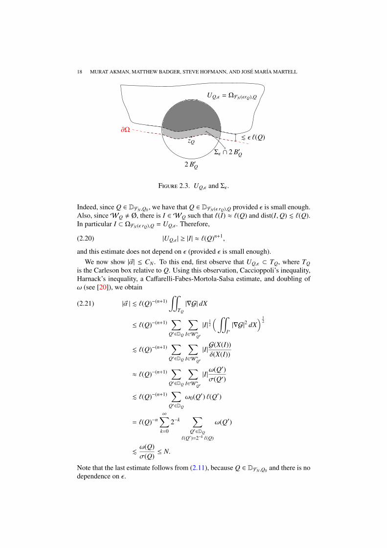
18 MURAT AKMAN, MATTHEW BADGER, STEVE HOFMANN, AND JOSE MARIA MARTELL
UQ,ε = ΩFN (εrQ),Q
zQ
∂Ω
Σε ∩ 2 B′Q
. ε `(Q)
2 B′Q
Figure 2.3. UQ,ε and Σε .
Indeed, since Q ∈ DFN ,Q0 , we have that Q ∈ DFN (ε rQ),Q provided ε is small enough.Also, sinceWQ , Ø, there is I ∈ WQ such that `(I) ≈ `(Q) and dist(I,Q) . `(Q).In particular I ⊂ ΩFN (ε rQ),Q = UQ,ε . Therefore,
|UQ,ε | ≥ |I| ≈ `(Q)n+1,(2.20)
and this estimate does not depend on ε (provided ε is small enough).We now show |~α| ≤ CN . To this end, first observe that UQ,ε ⊂ TQ, where TQ
is the Carleson box relative to Q. Using this observation, Caccioppoli’s inequality,Harnack’s inequality, a Caffarelli-Fabes-Mortola-Salsa estimate, and doubling ofω (see [20]), we obtain
|~α | . `(Q)−(n+1)"
TQ
|∇G| dX(2.21)
≤ `(Q)−(n+1)∑
Q′∈DQ
∑I∈W∗
Q′
|I|12
("I∗|∇G|2 dX
) 12
. `(Q)−(n+1)∑
Q′∈DQ
∑I∈W∗
Q′
|I|G(X(I))δ(X(I))
≈ `(Q)−(n+1)∑
Q′∈DQ
∑I∈W∗
Q′
|I|ω(Q′)σ(Q′)
. `(Q)−(n+1)∑
Q′∈DQ
ω0(Q′) `(Q′)
= `(Q)−n∞∑
k=0
2−k∑
Q′∈DQ
`(Q′)=2−k `(Q)
ω(Q′)
.ω(Q)σ(Q)
≤ N.
Note that the last estimate follows from (2.11), because Q ∈ DFN ,Q0 and there is nodependence on ε.
RECTIFIABILITY AND ELLIPTIC MEASURES 19
We are now ready to estimate II in (2.19). Recall that Q ∈ BN . By [16, Lemma5.7], failure of the η(N)-exterior Corkscrew property implies that |Ωext ∩ B′Q| .η(N) rn+1
Q . This and (2.21) give
(2.22) |II| . |~α | r−1Q |Ωext ∩ B′Q| . N η(N) rn
Q ≈ N η(N)σ(Q) <1
4 N C1σ(Q),
where in the last estimate we have chosen η(N) sufficiently small (η(N) ≤ (N2 M)−1
with M 1 depending only on the ADR and 1-sided NTA constants).We next estimate I. To start,
(2.23) |I| . r−1Q
( "(Ω\UQ,ε )∩B′Q
|∇G − ~α| dX +
"UQ,ε
|∇G − ~α| dX)
. `(Q)−1( "
B′Q∩Σε
|∇G − ~α| dX +
"UQ,ε
|∇G − ~α| dX)
=: `(Q)−1(I1 + I2).
Using [16, Lemma 5.9], we obtain
I1 . |~α| |B′Q ∩ Σε | +
"B′Q∩Σε
|∇G| dX . N ε `(Q)n+1 + I3 . N ε `(Q)σ(Q) + I3.
(2.24)
We estimate I3, as follows. Given I ∈ W, let Q∗I denote one of its nearest cubeswith `(Q∗I ) = `(I). Using the same ideas as in (2.21),
I3 ≤∑
I∈W:I∩B′Q,Ø`(I).ε `(Q)
"I|∇G| dX ≤
∑I∈W:I∩B′Q,Ø`(I).ε `(Q)
|I|12
("I|∇G| dX
) 12
.∑
I∈W:I∩B′Q,Ø`(I).ε `(Q)
|I|G(X(I))δ(X(I))
≈∑
I∈W:I∩B′Q,Ø`(I).ε `(Q)
|I|ω(Q∗I )σ(Q∗I )
.∑
I∈W:I∩B′Q,Ø`(I).ε `(Q)
ω(Q∗I ) `(I) =∑
k:2−k.ε `(Q)
2−k∑
I∈W:I∗∩B′Q,Ø
`(I)=2−k
ω(Q∗I ).
Note that if k is fixed, then the family Q∗I I∈W:`(I)=2−k has bounded overlap. Also,if I meets B′Q, then `(I) . rQ ≈ `(Q). Hence Q∗I ⊂ C ∆′Q = C B′Q ∩ ∂Ω for someuniform constant C. Thus,
I3 . ω(C ∆′Q)∑
k:2−k.ε `(Q)
2−k . ω(Q)ε `(Q) . N ε `(Q)σ(Q),(2.25)
where we used doubling of ω (see [20]) and Harnack’s inequality; moreover, in thelast estimate we invoked (2.11), since Q ∈ DFN ,Q0 . Gathering (2.23), (2.24), and(2.25), we obtain
|I| . N ε σ(Q) + `(Q)−1 I2 <1
4 N C1σ(Q) + `(Q)−1 I2(2.26)
20 MURAT AKMAN, MATTHEW BADGER, STEVE HOFMANN, AND JOSE MARIA MARTELL
provided we choose ε sufficiently small (ε ≤ (N2 M)−1 with M 1 depending onlyon the ADR and 1-sided NTA constants will suffice). For later use, we assume thatε = 2−Kε for some Kε ∈ N.
From (2.19), (2.22), and (2.26), it follows that
(C1 N)−1 σ(Q) ≤ |I| + |II| ≤1
2 N C1σ(Q) + `(Q)−1 I2.(2.27)
Upon rearranging the inequality, we conclude that
σ(Q) . 2 C1 N `(Q)I2.
Recall that at this point η(N) and ε = ε(N) are fixed and depend on N and the ADRand 1-sided NTA constants of Ω.
To continue with the previous estimate, we again use Harnack’s inequality, aCaffarelli-Fabes-Mortola-Salsa estimate and that ω is doubling (see [20]):
G(X)`(Q)
≈NG(X)δ(X)
≈Nω(Q)σ(Q)
≈N 1, ∀ X ∈ UQ,ε .
Then, invoking [19] (which contains a slight improvement of the Poincare inequal-ity proved in [16, Lemma 4.8]),
(2.28) σ(Q) .N `(Q)−1 |UQ,ε |12
("UQ,ε
|∇G − ~α|2 dX) 1
2
.N `(Q)n+1
2
("UQ,ε
|∇2G(X)|2 dX) 1
2≈N σ(Q)
12
("UQ,ε
|∇2G(X)|2 G(X)dX) 1
2.
Hiding this time σ(Q)12 , we conclude that
σ(Q) .N
"UQ,ε
|∇2G|2 G dX, ∀Q ∈ DFN ,Q0 ∩ BN .(2.29)
Recall that our goal is to obtain (2.18). Fix Q′0 ⊂ DQ0 . We may assume thatQ′0 ∈ DFN ,Q0 (otherwise m(DQ′0) = 0 and the desired estimate follows), in whichcase we have Q j ( Q′0 whenever Q′0 ∩ Q j , Ø. Hence
DF ′N ,Q′0 = DQ′0 ∩ DFN ,Q0 , where F ′N := Q j ∈ FN : Q j ( Q′0.
Recall that we chose ε to be of the form ε = 2−Kε for some Kε ∈ N. Let
F ?N :=
⋃Q∈F ′N
Q′ ∈ DQ : `(Q′) = 2−Kε`(Q) = ε`(Q)
.
Note that F ?N ⊂ DQ′0 and it is a disjoint family. For ease of notation, we let
Ω? := Ω∗DF?N ,Q′0
:= int( ⋃
Q∈DF?N ,Q′0
U∗Q)
:= int( ⋃
Q∈DF?N ,Q′0
⋃I∈W∗Q
I∗∗),
where I∗∗ = (1 + 2 λ) I. Thus,
(2.30)⋃
Q∈DF ′N ,Q′0
UQ,ε ⊂⋃
Q∈DF ′N ,Q′0
⋃Q′∈DQ
ε`(Q)<`(Q′)≤`(Q)
UQ ⊂⋃
Q∈DF?N ,Q′0
UQ
RECTIFIABILITY AND ELLIPTIC MEASURES 21
⊂ int( ⋃
Q∈DF?N ,Q′0
U∗Q)
= Ω?.
This, the fact that the family UQ,εQ∈D has have bounded overlap (depending on εand hence on N), see [1] or [19], and (2.29) yield
m(DQ′0) ≤∑
Q∈DQ′0Q∈DFN ,Q0∩B
N
σ(Q) .N
∑Q∈DF ′N ,Q
′0
"UQ,ε
|∇2G|2GdX .N
"Ω?
|∇2G|2GdX.
(2.31)
We now claim thatω(Q)σ(Q)
≈N 1, ∀Q ∈ DF ?N ,Q
′0.(2.32)
This is clear if Q ∈ DF ′N ,Q′0 ⊂ DFN ,Q0 by (2.11). Suppose next that Q ∈ DF ?N ,Q
′0\
DF ′N ,Q′0 . Then there is Q j ∈ F′N such that Q ⊂ Q j. We can split Q j into its ε-
descendants (recall that ε = 2−Kε ) and we can find Q′j ∈ F?N such that Q′j ∩ Q , Ø.
In turn, since Q ∈ DF ?N ,Q
′0, necessarily Q′j ( Q ⊂ Q j with `(Q′j) = ε `(Q j). Using
this, ADR, doubling of ω, and (2.11) which clearly holds for the father Q j of Q j,we conclude that
ω(Q)σ(Q)
≈Nω(Q j)
σ(Q j)≈N 1,
as desired.In order to integrate by parts, we need to get away from the boundary. To do
so, we introduce a large parameter M and define F ?N,M = F ?
N (2−M `(Q′0)); that is,F ?
N,M ⊂ DQ′0 is the family of maximal cubes of the collection F ?N augmented to
include all dyadic cubes of size smaller than or equal to 2−M `(Q0). In particular,Q ∈ DF ?
N,M ,Q′0
if and only if Q ∈ DF ?N ,Q
′0
and `(Q) > 2−M `(Q′0). Clearly, DF ?N,M ,Q
′0⊂
DF ?N,M′ ,Q
′0
if M ≤ M′, and therefore, Ω?M := Ω∗
F ?N,M ,Q
′0⊂ Ω∗
F ?N,M′ ,Q
′0⊂ Ω∗D
F?N ,Q′0= Ω?.
This and the monotone convergence theorem give"Ω?
|∇2G|2 G dX = limM→∞
"Ω?
M
|∇2G|2 G dX.(2.33)
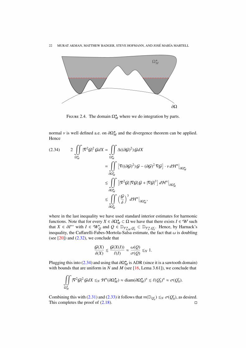
Thus, we may bound each of the right hand terms in (2.31) with bounds that areuniform in M using integration by parts (see Figure 2.4).
Fix M large. Note that Ω?M ⊂ Ω?
M ⊂ 2 BQ∗0 ∩Ω, and therefore, we again have theneeded PDE properties at our disposal. Let “∂” denote a fixed generic derivative.Easy calculations show that in 2 BQ∗0 ∩Ω we can use that G is harmonic and then
∆((∂G)2) = 2 div[(∂G)∇(∂G)] = 2 |∇(∂G)|2
and
∆((∂G)2)G = div[∇((∂G)2)G]−∇((∂G)2) · ∇G = div[∇((∂G)2)G]−div[(∂G)2∇G].
Since the domain Ω?M is comprised of a finite union of fattened Whitney cubes,
its boundary consists of portions of faces of those cubes. Thus, its (outward) unit
22 MURAT AKMAN, MATTHEW BADGER, STEVE HOFMANN, AND JOSE MARIA MARTELL
Ω?M
∂Ω
Figure 2.4. The domain Ω?M where we do integration by parts.
normal ν is well defined a.e. on ∂Ω?M and the divergence theorem can be applied.
Hence
2"Ω?
M
|∇2G|2 GdX =
"Ω?
M
∆((∂G)2)GdX(2.34)
=
"∂Ω?
M
[∇((∂G)2)G − (∂G)2 ∇G
]· ν dHn
∣∣∂Ω?
M
.
"∂Ω?
M
[|∇2G| |∇G| G + |∇G|3
]dHn
∣∣∂Ω?
M
.
"∂Ω?
M
(G
δ
)3dHn
∣∣∂Ω?
M,
where in the last inequality we have used standard interior estimates for harmonicfunctions. Note that for every X ∈ ∂Ω?
M ⊂ Ω we have that there exists I ∈ W suchthat X ∈ ∂I∗∗ with I ∈ W∗
Q and Q ∈ DF ?N,M ,Q
′0⊂ DF ?
N ,Q′0. Hence, by Harnack’s
inequality, the Caffarelli-Fabes-Mortola-Salsa estimate, the fact that ω is doubling(see [20]) and (2.32), we conclude that
G(X)δ(X)
.G(X(I))`(I)
≈ω(Q)σ(Q)
.N 1.
Plugging this into (2.34) and using that ∂Ω?M is ADR (since it is a sawtooth domain)
with bounds that are uniform in N and M (see [16, Lema 3.61]), we conclude that"Ω?
M
|∇2G|2 GdX .N Hn(∂Ω?
M) ≈ diam(∂Ω?M)n . `(Q′0)n ≈ σ(Q′0).
Combining this with (2.31) and (2.33) it follows thatm(DQ′0) .N σ(Q′0), as desired.This completes the proof of (2.18).
RECTIFIABILITY AND ELLIPTIC MEASURES 23
Equipped with the previous technical lemma, we immediately see that for everyQ′0 ∈ DFN ,Q0 there exists Q′′0 ∈ DQ′0 such that
2−CN`(Q′0) ≤ `(Q′′0 ) ≤ `(Q′0) and Q′′0 < DFN ,Q0 ∩ BN ,(2.35)
where CN is the constant in (2.18). Otherwise,
(CN + 1)σ(Q′0) =∑
Q∈DQ′02−CN `(Q′0)≤`(Q)≤`(Q′0)
σ(Q) ≤∑
Q∈DQ′0Q∈BN∩DFN ,Q0
σ(Q) ≤ CNσ(Q′0),
which is absurd.We now claim that
(2.36)
For all Q′0 ∈ DFN ,Q0 , there exists Q′0 ∈ DQ′0 such that
2−CN ≤`(Q′0)`(Q′0) ≤ 1 and either Q′0 ∈ FN or Q′0 < B
N .
To verify this claim, fix Q′0 ∈ DFN ,Q0 and let Q′′0 ∈ DQ′0 be a cube satisfying (2.35).We consider two separate possibilities.Case 1: Suppose that Q′′0 < DFN ,Q0 . Then there exists Q j ∈ FN such that Q′′0 ⊂ Q j.As a consequence, Q′′0 ⊂ Q j∩Q0 with Q′0 ∈ DFN ,Q0 give Q j ( Q′0. Thus, by (2.35),
Q′′0 ⊂ Q j ( Q′0 and 2−CN`(Q′0) ≤ `(Q′′0 ) ≤ `(Q j) ≤ `(Q′0).
In this case, we pick Q′0 := Q j.
Case 2: Suppose Q′′0 < BN . In this case, we let Q′0 := Q′′0 and the desired properties
follow at once from (2.35).We now have now all the ingredients required to prove Proposition 2.14, and
thus, complete the proof of (c) implies (d).
Proof of Proposition 2.14. By [16, Lemma 3.61], ΩFN ,Q0 is a 1-sided NTA withADR boundary. Hence all that remains is to show that ΩFN ,Q0 satisfies the exteriorcorkscrew condition with constant depending on N. Fix any point x ∈ ∂ΩFN ,Q0 and0 < r < diam(Q0) ≈ diam(ΩFN ,Q0). There are two cases.Case 1: Suppose that x ∈ ∂ΩFN ,Q0 with 0 ≤ δ(x) ≤ r/M, where M is large enough,to be chosen. We first note that there exists Q ∈ DQ0 with `(Q) ≈ r/M suchthat |x − xQ| . r/M. On one hand, if x ∈ ∂ΩFN ,Q0 ∩ ∂Ω, then x ∈ Q0 by (1.20)and we can find Q ∈ DQ0 with `(Q) ≈ r/M and x ∈ Q. On the other hand, ifx ∈ ∂ΩFN ,Q0 ∩ Ω, then by the definition of the sawtooth region, x ∈ ∂I∗, whereI ∈ W∗
Q′ , Q′ ∈ DFN ,Q0 , and |x − xQ′ | ≈ dist(I,Q′) ≈ `(Q′) ≈ `(I) ≈ δ(x) ≤ r/M.Let us now take Q ∈ DQ0 , an ancestor of Q′, such that `(Q) ≈ r/M and hence|x − xQ| ≤ |x − xQ′ | + |xQ′ − xQ| . r/M.
The proof now splits into two subcases.Case 1a: Suppose that Q < DFN ,Q0 . Then Q ⊂ Q j for some Q j ∈ FN and by[16, Lemma 5.9], there exists a ball B′ ⊂ Rn+1 \ ΩFN ,Q0 with center xQ and radiusr′ ≈ `(Q) ≈ r/M such that B′ ∩ ∂Ω ⊂ Q. If y ∈ B′, then we can guarantee
|y − x| ≤ |y − xQ| + |xQ − x| . r′ +`(Q)
M.`(Q)
M< r

24 MURAT AKMAN, MATTHEW BADGER, STEVE HOFMANN, AND JOSE MARIA MARTELL
by choosing M sufficiently large. Hence B′ ⊂ B(x, r) and xQ is an exterior cork-screw point relative to B(x, r) ∩ ∂ΩFN ,Q0 with corkscrew constant on the order ofM−1.Case 1b: Suppose that Q ∈ DFN ,Q0 . By (2.36), there exists Q ∈ DQ such that
2−CN ≤`(Q)`(Q)
≤ 1 and either Q ∈ FN or Q < BN .(2.37)
If Q ∈ FN , we argue as in Case 1a: [16, Lemma 5.9] gives a ball B′ ⊂ Rn+1\ΩFN ,Q0
with center xQ and radius r′ ≈ `(Q). Once again, B′ ⊂ B(x,C r/M) ⊂ B(x, r) if M islarge enough. Hence xQ is an exterior corkscrew point relative to B(x, r)∩∂ΩFN ,Q0
with corkscrew constant on the order of 2−CN M−1. Otherwise, if Q < BN , thenthe definition of BN yields zQ ∈ ∆Q ⊂ Q and X−
Qfor which B(X−
Q, η(N) `(Q)) ⊂
B(zQ, rQ/4) ∩ Ωext. Note that B(zQ, rQ/4) ⊂ B(x,C r/M) ⊂ B(x, r) provided M islarge enough. Hence X−
Qis an exterior corkscrew point relative to B(x, r)∩∂ΩFN ,Q0
with corkscrew constant of the order of 2−CN M−1.Case 2: Suppose that x ∈ ∂ΩFN ,Q0 with δ(x) > r/M. In particular, x ∈ Ω, and by thedefinition of the sawtooth region, x ∈ ∂I∗ ∩ J where I ∈ W∗
Q, Q ∈ DFN ,Q0 , J ∈ W,and τ J ⊂ Ω \ ΩFN ,Q0 for some τ ∈ (1/2, 1). Note that `(I) ≈ `(J) ≈ δ(x) > r/M.Hence we can easily find an exterior corkscrew point in the segment joining x withthe center of J and the corkscrew constant will depend only on M and the implicitconstants in the previous estimates.
This completes the proof that ΩFN ,Q0 satisfies the exterior corkscrew conditionwith constant depending on N.
2.5. Proof of (b) implies (e). Suppose (b) holds and let Ω? := ΩF ,Q0 be a chord-arc domain constructed in Section 2.2 in the proof of (b) implies (d). By [16,Proposition 6.4, Corollary 3.6], we can locate some AQ0 ∈ Ω∩Ω?, which is simul-taneously a Corkscrew point for Ω? with respect to B(x,C rQ0)∩Ω? for all x ∈ ∂Ω?
and a Corkscrew point for Ω with respect to B(x,C rQ0)∩Ω for all x ∈ Q0. To prove(e), it suffices to show that there exist constants θ, θ′ > 0 and C > 1 (possibly de-pending on Ω?) such that
(2.38) C−1σ(F)θ′
≤ ωAQ0 (F) ≤ C σ(F)θ ∀ F ⊂ Q0 \⋃
Q j∈F
Q j.
By Harnack’s inequality, one may replace AQ0 in (2.38) with some fixed pole X0 atthe expense of changing the value of C. We also remark that technically speakingwe should consider arbitrary sets F ⊂ ∂Ω∩∂Ω?. However, the general case followsfrom (2.38) in view of (1.20) and the fact that σ(∂Q) = ωAQ0 (∂Q) = 0 for everyQ ⊂ DQ0 , since σ and ωAQ0 are doubling (see [16, Proposition 6.3] and [19]).
Abusing notation, we let ω = ωAQ0 denote harmonic measure of Ω with pole atAQ0 and let ω? = ω
AQ0Ω?
denote harmonic measure of Ω? with pole at AQ0 . SinceΩ? is a chord-arc domain, ω? ∈ A∞(∂Ω?) by [11, 31]. In particular, there existconstants α, β such that(
σ?(E?)σ(∂Ω?)
)α.
ω?(E?)ω?(∂Ω?)
.
(σ?(E?)σ?(∂Ω?)
)β∀ E? ⊂ ∂Ω?,(2.39)
RECTIFIABILITY AND ELLIPTIC MEASURES 25
where σ? = Hn|∂Ω? , and we view ∂Ω? as a surface ball in ∂Ω? with arbitrarycenter in ∂Ω? and radius diam(∂Ω?). Recall that Ω? is a chord-arc domain and, inparticular, σ?(∂Ω?) ≈ diam(∂Ω?)n ≈ `(Q0)n.
We need to introduce some notation from [16, Section 6]. Given a Borel measureµ defined on Q0 and F from above, set
PF µ(E) := µ(
E \⋃
Q j∈F
Q j
)+∑Q j∈F
σ(E ∩ Q j)σ(Q j)
µ(Q j) ∀ E ⊂ Q0.(2.40)
Also, define a Borel measure on Q0 by the rule
ν(E) := ω?
(E \
⋃Q j∈F
Q j
)+∑Q j∈F
ω(E ∩ Q j)ω(Q j)
ω?(P j) ∀ E ⊂ Q0.(2.41)
Here P j ⊂ ∂Ω? are n-dimensional cubes from [16, Proposition 6.7], which satisfy
`(P j) ≈ dist(P j,Q j) ≈ dist(P j, ∂Ω) ≈ `(Q j) and∑
j
1P j ≤ C.(2.42)
From the definition of the projection operatorPF in (2.40) and measure ν in (2.41),
PF ν(E) = ω?(E \⋃
Q j∈F
Q j) +∑Q j∈F
σ(E ∩ Q j)σ(Q j)
ω?(P j) ∀ E ⊂ Q0,(2.43)
which depends only on ω? and not on ω.From [16, Lemma 6.15], we have the following version of the Dahlberg-Jerison-
Kenig sawtooth lemma (see [10]): There exists some θ > 0 such that for everyE ⊂ Q0, (
PFω(E)PFω(Q0)
)θ.PF ν(E)PF ν(Q0)
.PFω(E)PFω(Q0)
.(2.44)
Note that from (2.40) and (2.43), for every F ⊂ Q0\∪Q j we havePF ν(F) = ω?(F)and PFω(F) = ω(F). It is trivial to see that PFω(Q0) = ω(Q0) = ωAQ0 (Q0) ≈ 1 byBourgain’s estimate (see [7] or also [20]), since AQ0 is an effective Corkscrew pointrelative to Q0. Also, from (2.42) and (2.43) it is clear that PF ν(Q0) ≤ ω?(∂Ω?) =
1. Additionally, [16, Proposition 6.12, (6.19)], the fact that ω? is doubling (see[20]), and Bourgain’s estimate (see [7] or [20]) give
PF ν(Q0) & ω?(B(x?Q0,C `(Q0)) ∩ ∂Ω?) ≈ 1,
where x?Q0∈ ∂Ω? and we have used that AQ0 is an effective Corkscrew point relative
to B(x?Q0,C `(Q0)) ∩ ∂Ω? as noted above. All together, these observations plus
(1.20), (2.39) and (2.44) yield
σ(F)α . ω?(F) . ω(F) . ω?(F)1θ . σ(F)
βθ ∀ F ⊂ Q0 \
⋃Q j∈F
Q j,
as desired. We remark that the implicit constants depend on σ(∂Ω?) ≈ `(Q0)n.
26 MURAT AKMAN, MATTHEW BADGER, STEVE HOFMANN, AND JOSE MARIA MARTELL
3. Proof of Theorem 1.3
As noted in the introduction, to establish Theorem 1.3, it suffices to prove that(c’) implies (d) and (b) implies (e’). Before proceeding to the proof, we pause tomake a relevant remark.
Remark 3.1. The conditions on the coefficients of the operator in Theorem 1.3are qualitative versions of the corresponding conditions imposed in [24] and [19].Indeed, for every bounded subdomain Ω′ of Ω, the matrix A satisfies the conditionsimposed in [24] and [19] with respect to the domain Ω′. It is worth mentioning thatallowing implicit constants to depend on the subdomain Ω′ would be problematicin [24] and [19], where the authors are interested in establishing scale-invariantestimates. Nevertheless, we allow such dependence below, because our goal is toobtain qualitative rather than quantitative conditions.
3.1. Proof of (c’) implies (d). The proof follows the same scheme of Section 2.4and we only highlight the main changes. We replace ω, G and G by ωL, GL, GLthroughout Section 2.4. We note that thanks to [20] we have all the required “PDEproperties” such as Bourgain and Caffarelli-Fabes-Mortola-Salsa type estimates,doubling of elliptic measure, etc. However, one needs to rework the integration byparts (i.e. the main argument in Lemma 2.17), since now we work with L in placeof the Laplacian. Much as before we have the following substitute of (2.19):
(N C1)−1σL(Q) ≤ C−11 ωL(Q) ≤
∫∂Ω
φQ dω = −
"Ω
A∇GL · ∇φQ dX
= −
"Ω
(A∇GL − ~α) · ∇φQ dX +
"Ωext
~α · ∇φQ dX
=: −I + II,
where this time ~α := 1|UQ,ε |
!UQ,ε
A∇GLdX. From here the proof continues mutatis
mutandis (again with the help of [20] for the required “PDE properties”) and withthe harmless presence of the matrix A up to (2.28), which eventually leads to thefollowing variable coefficient version of (2.29):
σ(Q) .N
"UQ,ε
|∇(A∇GL)|2 GL dX ∀Q ∈ DFN ,Q0 ∩ BN .
Taking this into account and following the same argument, what is left to prove is
(3.2)"Ω?
M
|∇(A∇GL)|2 GLdX .N σ(Q′0)
with constants that do not depend on M. It was in that part of the proof where westrongly used harmonicity. However, (3.2) follows from the following “integrationby parts” proposition in [19].
Proposition 3.3 ([19]). Under the current background hypotheses and notation,and with Remark 3.1 in view, given Θ ≥ 1, and a family FK ⊂ DQ′0 , K ≥ 1, of
RECTIFIABILITY AND ELLIPTIC MEASURES 27
pairwise disjoint dyadic cubes satisfying
(3.4) Θ−1 ≤ωL(Q)σ(Q)
≤ Θ and `(Q) > 2−K `(Q′0) ∀Q ∈ DFK ,Q′0 ,
we then have
(3.5)1
σ(Q0)
"Ω∗FK ,Q
′0
∣∣∇(A∇GL)(X)|2 GL(X) dX ≤ C ,
where C depends on Θ and the allowable parameters, but not on K
Note that the constants in the analogue of (2.32) in the variable coefficient set-ting may depend on N and so does depend the implicit constant in (3.2). Thiscompletes the proof of the variable coefficient version of Lemma 2.17 . The restof the argument is of a geometrical nature and can be carried out without change.Details are left to the interested reader.
3.2. Proof of (b) implies (e’). We follow the arguments given in Section 2.5 aboveand indicate the necessary changes. To that end, set ωL = ω
AQ0L and ωL,? = ω
AQ0L,Ω?
,
which will replace ω = ωAQ0 and ω? = ωAQ0Ω?
, respectively.We claim that ωL,? ∈ A∞(∂Ω?). This is nowadays folklore and follows from the
fact that Ω? is a bounded chord-arc domain and from the properties of the matrix A.Let us sketch the argument for the sake of completeness. First recall that Kenig andPipher showed in [24] that if Ω is a bounded Lipschitz domain, then its associatedelliptic measure ωL,Ω ∈ A∞(∂Ω) provided that
aΩ
(X) = supY∈B(X,δ
Ω(X)/2)
|∇A(Y)|2 δΩ
(Y)
is a Carleson measure in Ω. Here δΩ
denotes the distance to ∂Ω. It is straightfor-ward to show that our assumptions on A give such a condition for every boundedsubdomain Ω ⊂ Ω, see Remark 3.1. On the other hand, since Ω? is a boundedchord-arc domain, Ω? satisfies an “interior big pieces” of Lipschitz sub-domainscondition by the work of David-Jerison in [11]. Together with a simple maximumprinciple argument (see e.g. in [9, 11]) and the aforementioned result of [24], onequickly obtains the following lower bound for ωL,Ω? : There are constants η ∈ (0, 1)and c0 > 0 such that for each surface ball ∆? ⊂ ∂Ω?, and any Borel subset F ⊂ ∆?,
(3.6) ωX∆?L,Ω?
(F) ≥ c0 , whenever σ?(F) ≥ ησ?(∆?).
In turn, the latter bound self-improves to an A∞ estimate for ωL,Ω? as desired, viathe comparison principle (see, e.g., [11]).
Once this claim has been obtained, the proof follows mutatis mutandis with aversion of (2.44) for L and with some needed PDE tools that can be taken from[20]. Details are left to the interested reader.
28 MURAT AKMAN, MATTHEW BADGER, STEVE HOFMANN, AND JOSE MARIA MARTELL
4. An example
As noted in the introduction, Theorem 1.2 can be seen as a qualitative versionof (1.1) in the sense that (a)–(e) can be seen as qualitative versions of (i)–(iv) in(1.1). In view of this, it is worthwhile to find an example of a domain Ω? satisfyingthe required background hypotheses (i.e., 1-sided NTA with ADR boundary), forwhich (a)–(e) in Theorem 1.2 hold, but (i)–(iv) in (1.1) fail. In particular, thecorresponding harmonic measure (or elliptic measures of the previous section) willsatisfy the absolute continuity conditions (c) and (e), but will not belong to A∞or weak-A∞. To find this example, we will start with Ω ⊂ R3, a 1-sided NTAdomain with empty exterior, whose boundary is not rectifiable. We will then definea sawtooth subdomain Ω? whose boundary is a countable union of partial facesof Whitney boxes. Therefore, ∂Ω? is rectifiable. On the other hand, we will seethat ∂Ω? cannot be Uniformly Rectifiable, otherwise Ω? is NTA and satisfies theexterior corkscrew condition by (1.1) (in particular, see [1]), but our constructionprevents this from happening.
Let C be the “4-corner Cantor set” of J. Garnett (see, e.g., [12, p. 4]). It isnot difficult to show from the construction of the set that R2 \ C is a 1-sided NTAdomain with 1-dimensional ADR boundary and empty exterior. Let C? = C × Rand Ω = R3 \C?. We shall show that Ω is a 1-sided NTA with 2-dimensional ADRboundary.
Let us first show that ∂Ω = C? is 2-dimensional ADR. Given x′ ∈ R2 and r > 0we write B2(x′, r) ⊂ R2 to denote the 2-dimensional ball centered at x′ with radiusr. Analogously, given t ∈ R and r > 0, B1(t, r) ⊂ R denotes the 1-dimensionalinterval centered at t with radius r. It is clear from the definition that for everyx = (x′, t) ∈ ∂Ω = C? one has(
B2(
x′, r/√
2)∩ C)× B1
(t, r/√
2)⊂ B(x, r) ∩ C? ⊂
(B2(x′, r) ∩ C
)× B1(t, r).
These readily imply that C? is 2-dimensional ADR as C is 1-dimensional ADR.We now recall that the complement of an ADR set always satisfies the Corkscrewcondition. In particular, so does R3\C? = Ω and this gives the (interior) Corkscrewcondition for Ω. We next show that Ω satisfies the Harnack Chain condition (inR3),again using that R2 \ C has the same property in R2. To this end let ρ > 0, Λ ≥ 1be given. Let X = (X′, t), Y = (Y ′, s) ∈ Ω, with X′, Y ′ ∈ R2 and t, s ∈ R. Note thatin particular X′, Y ′ ∈ R2 \ C. Assume that δ(X), δ(Y) > ρ and |X − Y | ≤ Λρ. It canbe easily seen that
δ(X) = dist(X, ∂Ω) = dist(X′,C) and δ(Y) = dist(Y, ∂Ω) = dist(Y ′,C).(4.1)
Using this observation and that R2 \ C satisfies the Harnack Chain condition in R2,we can find a Harnack Chain of 2-dimensional open balls connecting X′ and Y ′.The implicit constants are all under control and in particular the number of ballsdepends only on Λ by (4.1) and since |X′ − Y ′| ≤ |X − Y | ≤ Λ ρ. Now, for anyof the balls Bi
2 = B2(X′i , ri) ⊂ R2, we let Bi := B(Xi, ri) ⊂ R3 with Xi = (X′i , t).Clearly Bii is a Harnack chain in Ω connecting X = (X′, t) and Z := (Y ′, t). Nextwe can add to the previous chain a collection of 3-dimensional balls, connectingZ = (Y ′, t) with Y = (Y ′, s), whose centers lie in the line segment between Z and Yand with radius equal to δ(Y)/2 = dist(Y ′,C)/2. Note that the number of balls will
RECTIFIABILITY AND ELLIPTIC MEASURES 29
be of the order of |t − s|/δ(Y) ≤ |X − Y |/ρ ≤ Λ. Hence our proof of the HarnackChain condition is complete.
Now that we know Ω is a 1-sided NTA domain with ADR boundary, we simplynote that Ωext = Ø, which in particular implies (b) in Theorem 1.2 fails. Therefore,σ is not absolutely continuous with respect to ω by Theorem 1.2; that is, there is aset F ⊂ C? = ∂Ω with σ(F) > 0 but ω(F) = 0. Also, C? = ∂Ω is not rectifiable,again by Theorem 1.2.
Next, we are going to construct a pairwise disjoint family F ⊂ DQ0 with Q0 agiven dyadic cube in ∂Ω = C? and let Ω? = ΩF ,Q0 . As described above, we shallshow that
Ω? is 1-sided NTA,∂Ω? is ADR,∂Ω? is rectifiable,∂Ω? is not Uniformly Rectifiable.
(4.2)
Notice that in such a case ωΩ? will not be weak A∞(∂Ω?) by (1.1) (in particular,see [21]), but (a)–(e) in Theorem 1.2 hold, so in particular Hn
∣∣∂Ω? ωΩ? by (c)
and the two measures are mutually absolutely continuousHn∣∣∂Ω?
-a.e. by (e).
To construct our example, we let α0 ∈ N large enough so that 2−α0 < diam(∂Ω)and let αkk≥1 ⊂ N be an strictly increasing sequence such that αk → ∞ fastenough as k → ∞. Fix Q0 ∈ D such that `(Q0) = 2−α0 and set x0 = xQ0 its center.Take Q1 ∈ DQ0 such that x0 ∈ Q1 and `(Q1) = 2−α1 . Write x1 = xQ1 and set
F1 := Q ∈ DQ0 : `(Q) = 2−α1 , x0 < Q = Q ∈ DQ0 : `(Q) = 2−α1 \ Q1,
which is a pairwise disjoint family. Next, take Q2 ∈ DQ1 such that x1 ∈ Q2 and`(Q2) = 2−α2 . Let x2 = xQ2 denote the center of Q2 and set
F2 := Q ∈ DQ1 : `(Q) = 2−α2 , x1 < Q = Q ∈ DQ1 : `(Q) = 2−α2 \ Q2,
which is again a pairwise disjoint family. Iterating this we have a family of cubesQkk≥0 ⊂ DQ0 such that `(Qk) = 2−αk , and Q0 ) Q1 ) Q2 . . . and xk = xQk ∈ Qk+1.In particular, xkk≥1 is a Cauchy sequence (since αk → ∞ as k → ∞), and hence,there exists x ∈ ∂Ω such that xk → x as k → ∞. Note that
⋂k≥0 Qk = x.
Our construction also gives a family of pairwise disjoint families Fkk≥1 such thatF :=
⋃k≥1 Fk is a pairwise disjoint family of dyadic subcubes of Q0, and⋃
Q∈F
Q =
∞⋃k=1
⋃Q∈Fk
Q =
∞⋃k=1
(Qk−1 \ Qk) = Q0 \
∞⋂k=1
Qk.
At last, we set Ω? = ΩF ,Q0 (see Section 1). Because Ω is a 1-sided NTA domainwith ADR boundary, we know that Ω? is also a 1-sided NTA domain with ADRboundary by [16, Lemma 3.61]. It remains to show that ∂Ω? is rectifiable, but notUniformly Rectifiable.
To see that ∂Ω? is rectifiable, note that
∂Ω? = (∂Ω ∩ ∂Ω?) ∪ (Ω ∩ ∂Ω?).
30 MURAT AKMAN, MATTHEW BADGER, STEVE HOFMANN, AND JOSE MARIA MARTELL
On one hand, from (1.20), [16, Proposition 6.3], and the fact that ∂Ω is ADR (andhence σ = H2
∣∣∂Ω
is doubling), it follows that
σ(∂Ω ∩ ∂Ω?) = σ(
Q0 \⋃
Q∈F
Q)
= σ( ∞⋂
k=1
Qk
)= lim
k→∞σ(Qk) = 0,
where the last equality holds since σ(Qk) ≈ `(Qk)2 = 2−2αk → 0 as k → ∞. On theother hand, Ω ∩ ∂Ω? is countable union of partial faces of fattened Whitney cubesand hence Ω ∩ ∂Ω? is rectifiable (see the definition of sawtooth regions in Section1.3). Therefore, ∂Ω? is rectifiable.
Finally, we show that ∂Ω? is not Uniformly Rectifiable. Suppose otherwise that∂Ω? is Uniformly Rectifiable. Then, since Ω? is also a 1-sided NTA domain withADR boundary, we can apply (1.1) (in particular, the result of [1]) to conclude thatΩ? is an NTA domain. Therefore, Ω? satisfies the exterior corkscrew conditionwith some constant c0. In particular, for every x ∈ ∂Ω? and 0 < r < diam(∂Ω?) ≈`(Q0) = 2−α0 , there exists X∆? such that B(X∆? , c0 r) ⊂ B(x, r) ∩ (Ω?)ext, where∆? = B(x, r) ∩ ∂Ω?. Thus,
(4.3)|B(x, r) ∩ (Ω?)ext|
|B(x, r)|≥|B(X∆? , c0 r)||B(x, r)|
= cn0 ∀ x ∈ ∂Ω?, ∀ 0 < r . 2−α0 .
We are going to see that this is violated. Recall that xk → x as k → ∞ and thatxk ∈ ∂Ω ⊂ R3 \ Ω?. Also, for every k, we have that |XQk − xk| ≈ `(Qk) = 2−αk
and hence Xk → x as k → ∞. By construction, XQk ∈ int(UQk ) ⊂ Ω?, sinceQk ∈ DF ,Q0 . All together, these show that x ∈ ∂Ω?.
To get a contradiction we set Bk = B(x, 2−αk/N) with N ≥ 1 large enough tobe chosen (depending only on dimension and the 1-sided NTA and ADR constantsof Ω). Our goal is to obtain that (4.3) cannot hold, see Figure 4.1. Take X ∈(Bk ∩ Ω) \ Ω?. In particular, X ∈ Ω and we can take I ∈ W such that I 3 X and`(I) ≈ δ(X) ≤ 2−αk/N. Let QI ∈ D be the nearest cube to I with `(QI) = `(I) sothat I ∈ W∗
QI. Then, using the notation in (1.14),
|xQI − xk| . `(QI) + dist(QI , I) + `(I) + |X − x| + |x − xk+1| + |xk+1 − xk|
.2−αk
N+ diam(Qk+1) ≈
2−αk
N+ 2−αk+1 < rQk
by taking N large enough, because we have assumed that αk → ∞ fast enough.This implies that xQI ∈ ∆Qk ⊂ Qk, see (1.14). Also, `(QI) = `(I) . 2−αk/N <`(Qk), and by the dyadic properties, we conclude that QI ∈ DQk . In particular,observe that QI ∈ DQ0 . Since I ∈ W∗
QIand X < Ω? = ΩF ,Q0 , it follows that
QI < DF ,Q0 . In other words, QI ∈ DQ for some Q ∈ F =⋃
k≥1 Fk. Hence Q ∈ F j
for some j ≥ 1. By construction, QI ⊂ Q j−1 \ Q j. Thus, since QI ∈ DQk , it followsthat j ≥ k + 1 and δ(X) ≈ `(I) = `(QI) ≤ `(Q) ≤ 2−αk+1 . We have shown that
(Bk ∩Ω) \Ω? ⊂ Bk ∩ X < ∂Ω : δ(X) ≤ 2−αk+1.
Using (4.3) and [16, Lemma 5.3] (applied to E = ∂Ω, which is 2-dimensionalADR), we obtain a contradiction:
cn0 ≤|Bk \Ω?|
|Bk|=|(Bk ∩Ω) \Ω?|
|Bk|.
2−αk+1 (2−αk )2
(2−αk )3 = 2−(αk+1−αk) → 0
RECTIFIABILITY AND ELLIPTIC MEASURES 31
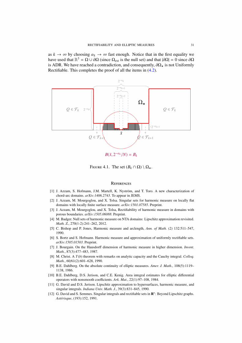
as k → ∞ by choosing αk → ∞ fast enough. Notice that in the first equality wehave used that R3 = Ω ∪ ∂Ω (since Ωext is the null set) and that |∂Ω| = 0 since ∂Ω
is ADR. We have reached a contradiction, and consequently, ∂Ω? is not UniformlyRectifiable. This completes the proof of all the items in (4.2).
Q ∈ Fk Q ∈ Fk
x
B(x, 2−αk/N) = Bk
Ω?
Q ∈ Fk+1 Q ∈ Fk+1
2−αk
2−αk
2−αk+1
2−αk+1
2−αk+2
Figure 4.1. The set (Bk ∩Ω) \Ω?.
References
[1] J. Azzam, S. Hofmann, J.M. Martell, K. Nystrom, and T. Toro. A new characterization ofchord-arc domains. arXiv:1406.2743. To appear in JEMS.
[2] J. Azzam, M. Mourgoglou, and X. Tolsa. Singular sets for harmonic measure on locally flatdomains with locally finite surface measure. arXiv:1501.07585. Preprint.
[3] J. Azzam, M. Mourgoglou, and X. Tolsa, Rectifiability of harmonic measure in domains withporous boundaries. arXiv:1505.06088. Preprint.
[4] M. Badger. Null sets of harmonic measure on NTA domains: Lipschitz approximation revisited.Math. Z., 270(1-2):241–262, 2012.
[5] C. Bishop and P. Jones, Harmonic measure and arclength, Ann. of Math. (2) 132:511–547,1990.
[6] S. Bortz and S. Hofmann. Harmonic measure and approximation of uniformly rectifiable sets.arXiv:1505.01503. Preprint.
[7] J. Bourgain. On the Hausdorff dimension of harmonic measure in higher dimension. Invent.Math., 87(3):477–483, 1987.
[8] M. Christ. A T (b) theorem with remarks on analytic capacity and the Cauchy integral. Colloq.Math., 60/61(2):601–628, 1990.
[9] B.E. Dahlberg. On the absolute continuity of elliptic measures. Amer. J. Math., 108(5):1119–1138, 1986.
[10] B.E. Dahlberg, D.S. Jerison, and C.E. Kenig. Area integral estimates for elliptic differentialoperators with nonsmooth coefficients. Ark. Mat., 22(1):97–108, 1984.
[11] G. David and D.S. Jerison. Lipschitz approximation to hypersurfaces, harmonic measure, andsingular integrals. Indiana Univ. Math. J., 39(3):831–845, 1990.
[12] G. David and S. Semmes. Singular integrals and rectifiable sets in Rn: Beyond Lipschitz graphs.Asterisque, (193):152, 1991.
32 MURAT AKMAN, MATTHEW BADGER, STEVE HOFMANN, AND JOSE MARIA MARTELL
[13] G. David and S. Semmes. Analysis of and on uniformly rectifiable sets, volume 38 of Mathe-matical Surveys and Monographs. American Mathematical Society, Providence, RI, 1993.
[14] D. Gilbarg and N. Trudinger, Elliptic Partial Differential Equations of Second Order, 2nd edi-tion, Springer-Verlag, Berlin 1983.
[15] S. Hofmann. P. Le, J.M. Martell, and K. Nystrom. Harmonic and p-harmonic measure, anduniform rectifiability. In preparation.
[16] S. Hofmann and J.M. Martell. Uniform rectifiability and harmonic measure I: uniform rectifia-bility implies Poisson kernels in Lp. Ann. Sci. Ec. Norm. Super. (4), 47(3):577–654, 2014.
[17] S. Hofmann and J.M. Martell. Uniform Rectifiability and harmonic measure IV: Ahlfors regu-larity plus Poisson kernels in Lp implies uniform rectifiability arXiv:1505.06499. Preprint.
[18] S. Hofmann, J.M. Martell, S. Mayboroda, X. Tolsa, and A. Volberg. Absolute continuity be-tween the surface measure and harmonic measure implies rectifiability. In preparation.
[19] S. Hofmann, J.M. Martell, and T. Toro. A characterization of chord-arc domains using ellipticmeasures. In preparation.
[20] S. Hofmann, J.M. Martell, and T. Toro. General divergence form elliptic operators on domainswith ADR boundaries, and on 1-sided NTA domains. In preparation.
[21] S. Hofmann, J.M. Martell, and I. Uriarte-Tuero. Uniform rectifiability and harmonic measure,II: Poisson kernels in Lp imply uniform rectifiability. Duke Math. J., 163(8):1601–1654, 2014.
[22] S. Hofmann, D. Mitrea, M. Mitrea, and A.J. Morris. Lp-square function estimates on spaces ofhomogeneous type and on uniformly rectifiable sets. arXiv:1301.4943. To appear in MemoirAMS.
[23] D.S. Jerison and C.E. Kenig. Boundary behavior of harmonic functions in non-tangentiallyaccessible domains. Adv. in Math., 46(1):80–147, 1982.
[24] C.E. Kenig and J. Pipher. The Dirichlet problem for elliptic equations with drift terms. Publ.Mat., 45:199–217, 2001.
[25] M. Lavrentiev. Boundary problems in the theory of univalent functions. Amer. Math. Soc.Transl. (2), 32:1–35, 1963.
[26] J.L. Lewis and K. Nystrom. Regularity and free boundary regularity for the p-Laplace operatorin Reifenberg flat and Ahlfors regular domains. J. Amer. Math. Soc., 25(3):827–862, 2012.
[27] P. Mattila. Geometry of sets and measures in Euclidean spaces, volume 44 of Cambridge Stud-ies in Advanced Mathematics. Cambridge University Press, Cambridge, 1995. Fractals andrectifiability.
[28] M. Mourgoglou, Uniform domains with rectifiable boundaries and harmonic measure,arXiv:1505.06167. Preprint.
[29] F. Nazarov, X. Tolsa, and A. Volberg. On the uniform rectifiability of AD-regular measureswith bounded Riesz transform operator: the case of codimension 1, Acta Math. 213(2):237–321, 2014.
[30] F. Nazarov, X. Tolsa and A. Volberg. The Riesz transform, rectifiability, and removability forLipschitz harmonic functions. Publ. Mat. 58:517–532, 2014.
[31] S. Semmes. Analysis vs. geometry on a class of rectifiable hypersurfaces in Rn. Indiana Univ.Math. J., 39(4):1005–1035, 1990.
[32] J.-M. Wu. On singularity of harmonic measure in space. Pacific J. Math., 121(2):485–496,1986.
[33] W.P. Ziemer. Some remarks on harmonic measure in space. Pacific J. Math., 55:629–637, 1974.
RECTIFIABILITY AND ELLIPTIC MEASURES 33
Murat Akman, Instituto de Ciencias Matematicas CSIC-UAM-UC3M-UCM, Consejo Superior
de Investigaciones Cientıficas, C/ Nicolas Cabrera, 13-15, E-28049 Madrid, Spain
E-mail address: [email protected]
Matthew Badger, Department of Mathematics, University of Connecticut, Storrs, CT 06269-3009, USA
E-mail address: [email protected]
Steve Hofmann, Department of Mathematics, University of Missouri, Columbia, MO 65211,USA
E-mail address: [email protected]
Jose Marıa Martell, Instituto de Ciencias Matematicas CSIC-UAM-UC3M-UCM, Consejo Su-perior de Investigaciones Cientıficas, C/ Nicolas Cabrera, 13-15, E-28049 Madrid, Spain
E-mail address: [email protected]