· Recap Geom CE HT Dual Potts Chrom Markov Cont Trunc Penr Geometrical polymer models Original...
156
Recap Geom CE HT Dual Potts Chrom Markov Cont Trunc Penr Cluster expansions for hard-core systems. II. Overview (end) and convergence criteria Roberto Fern´ andez CNRS - Universit´ e de Rouen Kac seminar, March 2008
Transcript of · Recap Geom CE HT Dual Potts Chrom Markov Cont Trunc Penr Geometrical polymer models Original...

Recap Geom CE HT Dual Potts Chrom Markov Cont Trunc Penr
Cluster expansionsfor hard-core systems.
II. Overview (end)and convergence criteria
Roberto FernandezCNRS - Universite de Rouen
Kac seminar, March 2008

Recap Geom CE HT Dual Potts Chrom Markov Cont Trunc Penr
The setup
Ingredients
I Countable family P of objects: polymers, animals, . . .I Incompatibility constraint: γ γ′ (with γ γ)I Activities z = zγγ∈P ∈ CP .
The basic (“finite-volume”) measuresFor each finite family PΛ ⊂ P
WΛ
(γ1, γ2, . . . , γn
)=
1ΞΛ(z)
zγ1zγ2 · · · zγn
∏j<k
11γj∼γk
ΞΛ(z) = 1 +∑n≥1
1n!
∑(γ1,...,γn)∈Pn
Λ
zγ1zγ2 . . . zγn
∏j<k
11γj∼γk
Recap Geom CE HT Dual Potts Chrom Markov Cont Trunc Penr
Graph-theoretical framework
Incompatibility graph G = (P, E)
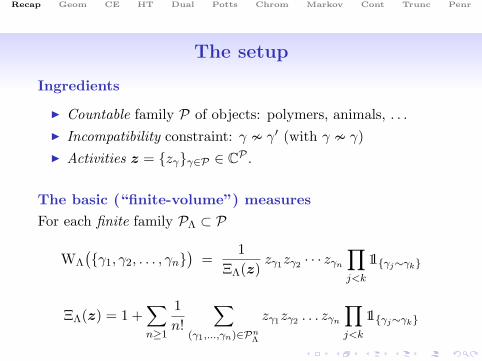
I Incompatible = neighboring (γ γ′ ≡ γ ↔ γ′)I Polymer system = hard-core gas in a complicated latticeI N ∗
γ0= γ ∈ P : γ γ0; Nγ0 = N ∗
γ0\ γ0
I Independent vertices = non-neighboring verticesI Independent sets = sets formed by independent vertices
Thus,ΞΛ(z) =
∑Γ⊂PΛ
independent
zΓ with zΓ =∏γ∈Γ
zγ
Recap Geom CE HT Dual Potts Chrom Markov Cont Trunc Penr
Graph-theoretical framework
Incompatibility graph G = (P, E)
I Incompatible = neighboring (γ γ′ ≡ γ ↔ γ′)I Polymer system = hard-core gas in a complicated latticeI N ∗
γ0= γ ∈ P : γ γ0; Nγ0 = N ∗
γ0\ γ0
I Independent vertices = non-neighboring verticesI Independent sets = sets formed by independent vertices
Thus,ΞΛ(z) =
∑Γ⊂PΛ
independent
zΓ with zΓ =∏γ∈Γ
zγ
Recap Geom CE HT Dual Potts Chrom Markov Cont Trunc Penr
Ratios of partition functions
I Correlations:
ProbΛ
(γ1, . . . , γk are present
)= zγ1 · · · zγk
ΞΛ\γ1,...,γk∗
ΞΛ
I Characteristic functions: If SΛ(γ1, . . . , γn) =∑n
i=1 α(γi)
EΛ
(eξ SΛ
)=
ΞΛ(zξ)ΞΛ(z)
with zξγ = zγ eξα(γ)
I Zeros of partition functions related to smoothness of
f(β,h) = limΛ→L
1|Λ|
logZσΛ

Recap Geom CE HT Dual Potts Chrom Markov Cont Trunc Penr
Previous example: Single-call loss networks
I P = finite connected families of links of Zd —the callsI zγ = Poissonian rate for the call γI Compatibility = use of disjoint links (no intersection)I Basic measures are invariant for the finite-region processI Thermodynamic limit: infinite-volume process
Recap Geom CE HT Dual Potts Chrom Markov Cont Trunc Penr
Previous example: Ising model at low T
Using the contour representation:I Polymers = contours (connected closed surfaces)I Compatibility = no intersectionI zγ = exp−2βJ |γ|
ThenWΛ(ω | +) =
1ΞΛ
∏γ∈Γ(ω)
zγ
with
ΞΛ(z) = 1 +∑n≥1
1n!
∑(γ1,...,γn)∈Cn
Λ
zγ1zγ2 . . . zγn
∏j<k
11γj∼γk
Recap Geom CE HT Dual Potts Chrom Markov Cont Trunc Penr
Previous example: LTE for Ising ferromagnets
WriteHΛ(ω) = −
∑B∈BΛ
JB
(ωB − 1
)−
∑B∈BΛ
JB
I Contour = connected component of (excited) bondsI zγ = exp
−2β
∑B∈γ JB
I γ ∼ γ′ iff γ ∩ γ′ = ∅ (disjoint bases); γ = ∪B : B ∈ γ
Then ZΛ = |SΛ| ΞLTΛ with
SΛ =χ : χB = 1 for all B ∈ BΛ
(symmetry group) and
ΞLTΛ (z) = 1 +
∑n≥1
1n!
∑(γ1,...,γn)∈Cn
Λ
zγ1zγ2 . . . zγn
∏j<k
11γj∼γk

Recap Geom CE HT Dual Potts Chrom Markov Cont Trunc Penr
Geometrical polymer models
Original polymer models of Gruber and Kunz:
I P = family of finite subsets of some set VI γ ∼ γ′ ⇐⇒ γ ∩ γ′ = ∅
UsuallyI V = vertex set of a graph (lattice, dual lattice)I Polymers defined by connectivity propertiesI Compatibility determined by graph distances
Warning: Do not confuse with the incompatibility graph
A little more general: decorated geometrical polymers
γ = (γ,Dγ) , γ = “base” ⊂⊂ V , Dγ = “decoration”
Recap Geom CE HT Dual Potts Chrom Markov Cont Trunc Penr
Cluster expansions
Write the polynomials (in (zγ)γ∈P)
ΞΛ(z) = 1 +∑n≥1
1n!
∑(γ1,...,γn)∈Pn
Λ
zγ1zγ2 . . . zγn
∏j<k
11γj∼γk
as formal exponentials of a formal series
ΞΛ(z) F= exp ∞∑
n=1
1n!
∑(γ1,...,γn)∈Pn
Λ
φT (γ1, . . . , γn) zγ1 . . . zγn
I The series between curly brackets is the cluster expansionI φT (γ1, . . . , γn): Ursell or truncated functions (symmetric)I Clusters: Families γ1, . . . , γn s.t. φT (γ1, . . . , γn) 6= 0I Clusters are connected w.r.t. “”

Recap Geom CE HT Dual Potts Chrom Markov Cont Trunc Penr
Classical cluster-expansion strategy
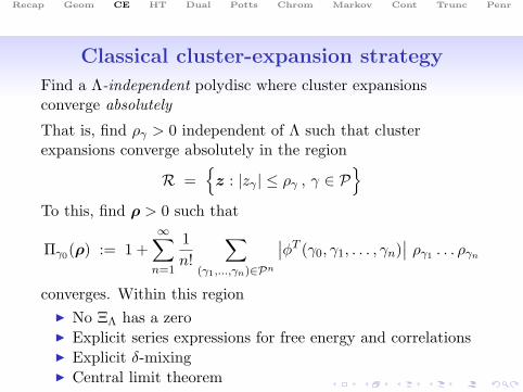
Find a Λ-independent polydisc where cluster expansionsconverge absolutely
That is, find ργ > 0 independent of Λ such that clusterexpansions converge absolutely in the region
R =
z : |zγ | ≤ ργ , γ ∈ P
To this, find ρ > 0 such that
Πγ0(ρ) := 1 +∞∑
n=1
1n!
∑(γ1,...,γn)∈Pn
∣∣φT (γ0, γ1, . . . , γn)∣∣ ργ1 . . . ργn
converges. Within this regionI No ΞΛ has a zeroI Explicit series expressions for free energy and correlationsI Explicit δ-mixingI Central limit theorem
Recap Geom CE HT Dual Potts Chrom Markov Cont Trunc Penr
Classical cluster-expansion strategy
Find a Λ-independent polydisc where cluster expansionsconverge absolutely
That is, find ργ > 0 independent of Λ such that clusterexpansions converge absolutely in the region
R =
z : |zγ | ≤ ργ , γ ∈ P
To this, find ρ > 0 such that
Πγ0(ρ) := 1 +∞∑
n=1
1n!
∑(γ1,...,γn)∈Pn
∣∣φT (γ0, γ1, . . . , γn)∣∣ ργ1 . . . ργn
converges. Within this regionI No ΞΛ has a zeroI Explicit series expressions for free energy and correlationsI Explicit δ-mixingI Central limit theorem
Recap Geom CE HT Dual Potts Chrom Markov Cont Trunc Penr
Associated polymer models
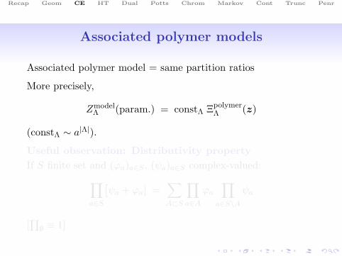
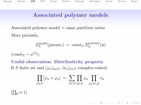
Associated polymer model = same partition ratios
More precisely,
ZmodelΛ (param.) = constΛ Ξpolymer
Λ (z)
(constΛ ∼ a|Λ|).
Useful observation: Distributivity propertyIf S finite set and (ϕa)a∈S , (ψa)a∈S complex-valued:∏
a∈S
[ψa + ϕa] =
∑A⊂S
∏a∈A
ϕa
∏a∈S\A
ψa
[∏∅ ≡ 1]
Recap Geom CE HT Dual Potts Chrom Markov Cont Trunc Penr
Associated polymer models
Associated polymer model = same partition ratios
More precisely,
ZmodelΛ (param.) = constΛ Ξpolymer
Λ (z)
(constΛ ∼ a|Λ|).
Useful observation: Distributivity propertyIf S finite set and (ϕa)a∈S , (ψa)a∈S complex-valued:∏
a∈S
[ψa + ϕa] =
∑A⊂S
∏a∈A
ϕa
∏a∈S\A
ψa
[∏∅ ≡ 1]
Recap Geom CE HT Dual Potts Chrom Markov Cont Trunc Penr
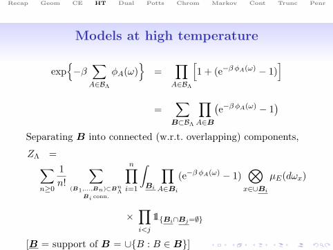
Models at high temperature
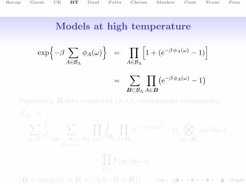
exp−β
∑A∈BΛ
φA(ω)
=∏
A∈BΛ
[1 + (e−β φA(ω) − 1)
]
=∑
B⊂BΛ
∏A∈B
(e−β φA(ω) − 1
)Separating B into connected (w.r.t. overlapping) components,
ZΛ =∑n≥0
1n!
∑(B1,...,Bn)⊂Bn
ΛBi conn.
n∏i=1
∫Bi
∏A∈Bi
(e−β φA(ω) − 1)⊗
x∈∪Bi
µE(dωx)
×∏i<j
11Bi∩Bj=∅
[B = support of B = ∪B : B ∈ B]
Recap Geom CE HT Dual Potts Chrom Markov Cont Trunc Penr
Models at high temperature
exp−β
∑A∈BΛ
φA(ω)
=∏
A∈BΛ
[1 + (e−β φA(ω) − 1)
]
=∑
B⊂BΛ
∏A∈B
(e−β φA(ω) − 1
)Separating B into connected (w.r.t. overlapping) components,
ZΛ =∑n≥0
1n!
∑(B1,...,Bn)⊂Bn
ΛBi conn.
n∏i=1
∫Bi
∏A∈Bi
(e−β φA(ω) − 1)⊗
x∈∪Bi
µE(dωx)
×∏i<j
11Bi∩Bj=∅
[B = support of B = ∪B : B ∈ B]
Recap Geom CE HT Dual Potts Chrom Markov Cont Trunc Penr
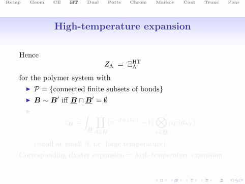
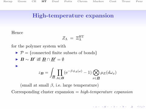
High-temperature expansion
HenceZΛ = ΞHT
Λ
for the polymer system withI P = connected finite subsets of bondsI B ∼ B′ iff B ∩B′ = ∅I
zB =∫
B
∏A∈B
(e−β φA(ω) − 1)⊗x∈B
µE(dωx)
(small at small β, i.e. large temperature)Corresponding cluster expansion = high-temperature expansion
Recap Geom CE HT Dual Potts Chrom Markov Cont Trunc Penr
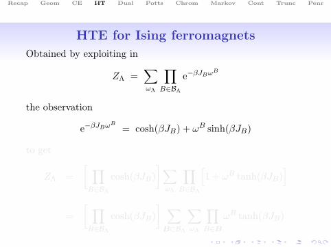
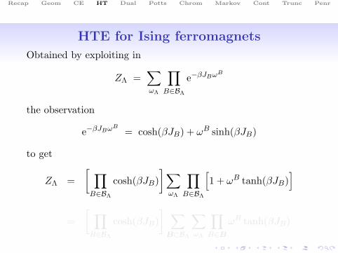
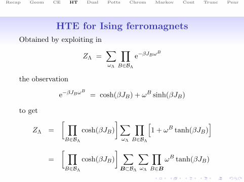
HTE for Ising ferromagnets
Obtained by exploiting in
ZΛ =∑ωΛ
∏B∈BΛ
e−βJBωB
the observation
e−βJBωB= cosh(βJB) + ωB sinh(βJB)
to get
ZΛ =[ ∏
B∈BΛ
cosh(βJB)]∑
ωΛ
∏B∈BΛ
[1 + ωB tanh(βJB)
]
=[ ∏
B∈BΛ
cosh(βJB)] ∑
B⊂BΛ
∑ωΛ
∏B∈B
ωB tanh(βJB)
Recap Geom CE HT Dual Potts Chrom Markov Cont Trunc Penr
HTE for Ising ferromagnets
Obtained by exploiting in
ZΛ =∑ωΛ
∏B∈BΛ
e−βJBωB
the observation
e−βJBωB= cosh(βJB) + ωB sinh(βJB)
to get
ZΛ =[ ∏
B∈BΛ
cosh(βJB)]∑
ωΛ
∏B∈BΛ
[1 + ωB tanh(βJB)
]
=[ ∏
B∈BΛ
cosh(βJB)] ∑
B⊂BΛ
∑ωΛ
∏B∈B
ωB tanh(βJB)
Recap Geom CE HT Dual Potts Chrom Markov Cont Trunc Penr
HTE for Ising ferromagnets
Obtained by exploiting in
ZΛ =∑ωΛ
∏B∈BΛ
e−βJBωB
the observation
e−βJBωB= cosh(βJB) + ωB sinh(βJB)
to get
ZΛ =[ ∏
B∈BΛ
cosh(βJB)]∑
ωΛ
∏B∈BΛ
[1 + ωB tanh(βJB)
]
=[ ∏
B∈BΛ
cosh(βJB)] ∑
B⊂BΛ
∑ωΛ
∏B∈B
ωB tanh(βJB)
Recap Geom CE HT Dual Potts Chrom Markov Cont Trunc Penr
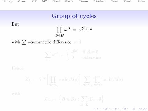
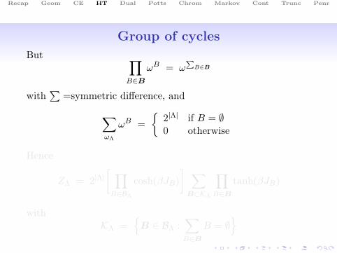
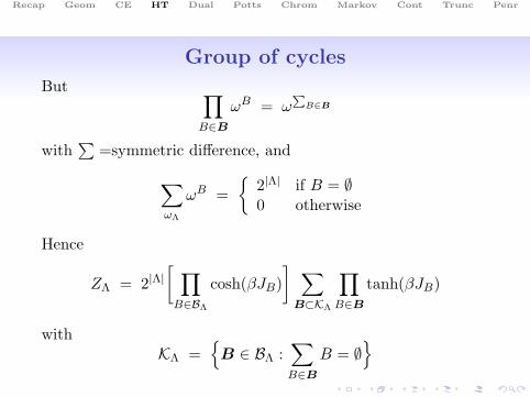
Group of cycles
But ∏B∈B
ωB = ωP
B∈B
with∑
=symmetric difference, and∑ωΛ
ωB =
2|Λ| if B = ∅0 otherwise
Hence
ZΛ = 2|Λ|[ ∏
B∈BΛ
cosh(βJB)] ∑
B⊂KΛ
∏B∈B
tanh(βJB)
withKΛ =
B ∈ BΛ :
∑B∈B
B = ∅
Recap Geom CE HT Dual Potts Chrom Markov Cont Trunc Penr
Group of cycles
But ∏B∈B
ωB = ωP
B∈B
with∑
=symmetric difference, and∑ωΛ
ωB =
2|Λ| if B = ∅0 otherwise
Hence
ZΛ = 2|Λ|[ ∏
B∈BΛ
cosh(βJB)] ∑
B⊂KΛ
∏B∈B
tanh(βJB)
withKΛ =
B ∈ BΛ :
∑B∈B
B = ∅
Recap Geom CE HT Dual Potts Chrom Markov Cont Trunc Penr
Group of cycles
But ∏B∈B
ωB = ωP
B∈B
with∑
=symmetric difference, and∑ωΛ
ωB =
2|Λ| if B = ∅0 otherwise
Hence
ZΛ = 2|Λ|[ ∏
B∈BΛ
cosh(βJB)] ∑
B⊂KΛ
∏B∈B
tanh(βJB)
withKΛ =
B ∈ BΛ :
∑B∈B
B = ∅

Recap Geom CE HT Dual Potts Chrom Markov Cont Trunc Penr
Ferromagnetic HT polymer model
The maximally connected elements of KΛ are the cycles
(KΛ is a group for “∑
”, generated by the cycles)
Factorizing the contribution of cycles,
ZΛ = 2|Λ|[ ∏
B∈BΛ
cosh(βJB)]ΞIHT
Λ
for the polymer system withI Polymers P = cyclesI Consistency: B ∼ B′ iff B ∩B′ = ∅I Fugacities (small at small β)
zB =∏
B∈B
tanh(βJB)
Recap Geom CE HT Dual Potts Chrom Markov Cont Trunc Penr
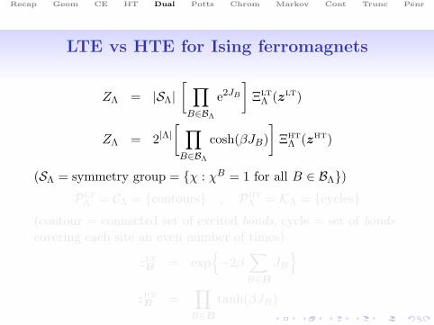
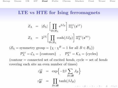
LTE vs HTE for Ising ferromagnets
ZΛ = |SΛ|[ ∏
B∈BΛ
e2JB
]ΞLT
Λ (zLT)
ZΛ = 2|Λ|[ ∏
B∈BΛ
cosh(βJB)]
ΞHTΛ (zHT)
(SΛ = symmetry group = χ : χB = 1 for all B ∈ BΛ)PLT
Λ = CΛ = contours , PHTΛ = KΛ = cycles
(contour = connected set of excited bonds, cycle = set of bondscovering each site an even number of times)
zLTB = exp
−2β
∑B∈B
JB
zHTB =
∏B∈B
tanh(βJB)

Recap Geom CE HT Dual Potts Chrom Markov Cont Trunc Penr
LTE vs HTE for Ising ferromagnets
ZΛ = |SΛ|[ ∏
B∈BΛ
e2JB
]ΞLT
Λ (zLT)
ZΛ = 2|Λ|[ ∏
B∈BΛ
cosh(βJB)]
ΞHTΛ (zHT)
(SΛ = symmetry group = χ : χB = 1 for all B ∈ BΛ)PLT
Λ = CΛ = contours , PHTΛ = KΛ = cycles
(contour = connected set of excited bonds, cycle = set of bondscovering each site an even number of times)
zLTB = exp
−2β
∑B∈B
JB
zHTB =
∏B∈B
tanh(βJB)
Recap Geom CE HT Dual Potts Chrom Markov Cont Trunc Penr
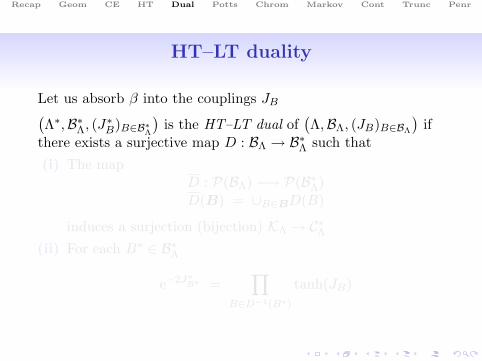
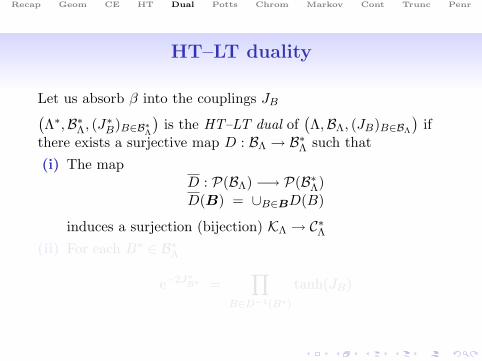
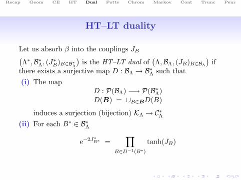
HT–LT duality
Let us absorb β into the couplings JB(Λ∗,B∗Λ, (J∗B)B∈B∗Λ
)is the HT–LT dual of
(Λ,BΛ, (JB)B∈BΛ
)if
there exists a surjective map D : BΛ → B∗Λ such that(i) The map
D : P(BΛ) −→ P(B∗Λ)D(B) = ∪B∈BD(B)
induces a surjection (bijection) KΛ → C∗Λ(ii) For each B∗ ∈ B∗Λ
e−2J∗B∗ =
∏B∈D−1(B∗)
tanh(JB)
Recap Geom CE HT Dual Potts Chrom Markov Cont Trunc Penr
HT–LT duality
Let us absorb β into the couplings JB(Λ∗,B∗Λ, (J∗B)B∈B∗Λ
)is the HT–LT dual of
(Λ,BΛ, (JB)B∈BΛ
)if
there exists a surjective map D : BΛ → B∗Λ such that(i) The map
D : P(BΛ) −→ P(B∗Λ)D(B) = ∪B∈BD(B)
induces a surjection (bijection) KΛ → C∗Λ(ii) For each B∗ ∈ B∗Λ
e−2J∗B∗ =
∏B∈D−1(B∗)
tanh(JB)

Recap Geom CE HT Dual Potts Chrom Markov Cont Trunc Penr
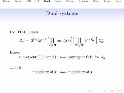
Dual systems
For HT–LT duals
ZΛ = 2|Λ| |S|−1[ ∏B∈B
cosh(JB)][ ∏
B∗∈B∗
e−2J∗B∗
]Z∗Λ∗
Hence:convergent C.E. for Z∗Λ∗ ⇐⇒ convergent C.E. for ZΛ
That is,analyticity of f∗ ⇐⇒ analyticity of f
Recap Geom CE HT Dual Potts Chrom Markov Cont Trunc Penr
Dual systems
For HT–LT duals
ZΛ = 2|Λ| |S|−1[ ∏B∈B
cosh(JB)][ ∏
B∗∈B∗
e−2J∗B∗
]Z∗Λ∗
Hence:convergent C.E. for Z∗Λ∗ ⇐⇒ convergent C.E. for ZΛ
That is,analyticity of f∗ ⇐⇒ analyticity of f

Recap Geom CE HT Dual Potts Chrom Markov Cont Trunc Penr
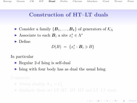
Construction of HT–LT duals
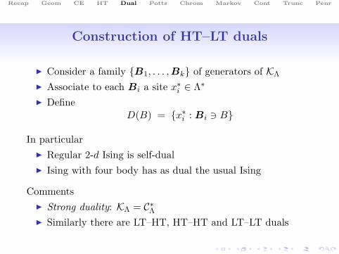
I Consider a family B1, . . . ,Bk of generators of KΛ
I Associate to each Bi a site x∗i ∈ Λ∗
I DefineD(B) = x∗i : Bi 3 B
In particularI Regular 2-d Ising is self-dualI Ising with four body has as dual the usual Ising
CommentsI Strong duality: KΛ = C∗ΛI Similarly there are LT–HT, HT–HT and LT–LT duals
Recap Geom CE HT Dual Potts Chrom Markov Cont Trunc Penr
Construction of HT–LT duals
I Consider a family B1, . . . ,Bk of generators of KΛ
I Associate to each Bi a site x∗i ∈ Λ∗
I DefineD(B) = x∗i : Bi 3 B
In particularI Regular 2-d Ising is self-dualI Ising with four body has as dual the usual Ising
CommentsI Strong duality: KΛ = C∗ΛI Similarly there are LT–HT, HT–HT and LT–LT duals
Recap Geom CE HT Dual Potts Chrom Markov Cont Trunc Penr
Potts model
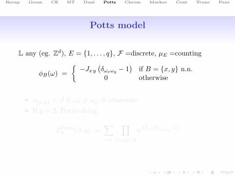
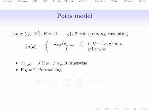
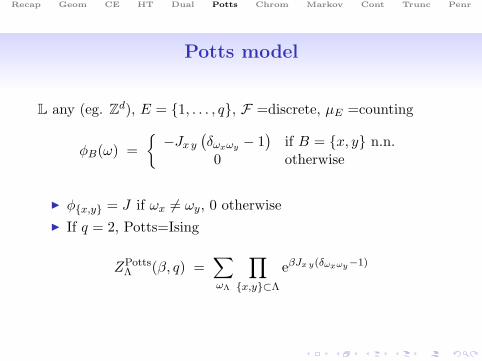
L any (eg. Zd), E = 1, . . . , q, F =discrete, µE =counting
φB(ω) =−Jx y
(δωxωy − 1
)if B = x, y n.n.
0 otherwise
I φx,y = J if ωx 6= ωy, 0 otherwiseI If q = 2, Potts=Ising
ZPottsΛ (β, q) =
∑ωΛ
∏x,y⊂Λ
eβJx y(δωxωy−1)
Recap Geom CE HT Dual Potts Chrom Markov Cont Trunc Penr
Potts model
L any (eg. Zd), E = 1, . . . , q, F =discrete, µE =counting
φB(ω) =−Jx y
(δωxωy − 1
)if B = x, y n.n.
0 otherwise
I φx,y = J if ωx 6= ωy, 0 otherwiseI If q = 2, Potts=Ising
ZPottsΛ (β, q) =
∑ωΛ
∏x,y⊂Λ
eβJx y(δωxωy−1)
Recap Geom CE HT Dual Potts Chrom Markov Cont Trunc Penr
Potts model
L any (eg. Zd), E = 1, . . . , q, F =discrete, µE =counting
φB(ω) =−Jx y
(δωxωy − 1
)if B = x, y n.n.
0 otherwise
I φx,y = J if ωx 6= ωy, 0 otherwiseI If q = 2, Potts=Ising
ZPottsΛ (β, q) =
∑ωΛ
∏x,y⊂Λ
eβJx y(δωxωy−1)
Recap Geom CE HT Dual Potts Chrom Markov Cont Trunc Penr
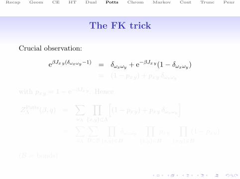
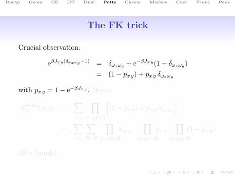
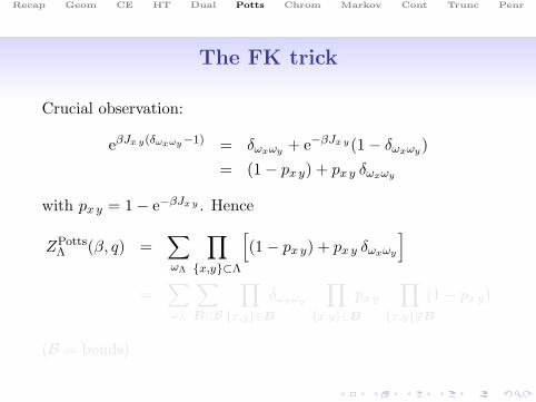
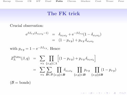
The FK trick
Crucial observation:
eβJx y(δωxωy−1) = δωxωy + e−βJx y(1− δωxωy)= (1− px y) + px y δωxωy
with px y = 1− e−βJx y . Hence
ZPottsΛ (β, q) =
∑ωΛ
∏x,y⊂Λ
[(1− px y) + px y δωxωy
]=
∑ωΛ
∑B⊂B
∏x,y∈B
δωxωy
∏x,y∈B
px y
∏x,y6∈B
(1− px y)
(B = bonds)
Recap Geom CE HT Dual Potts Chrom Markov Cont Trunc Penr
The FK expansion
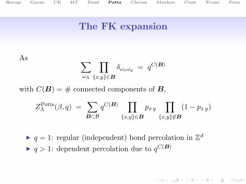
As ∑ωΛ
∏x,y∈B
δωxωy = qC(B)
with C(B) = # connected components of B,
ZPottsΛ (β, q) =
∑B⊂B
qC(B)∏
x,y∈B
px y
∏x,y6∈B
(1− px y)
I q = 1: regular (independent) bond percolation in Zd
I q > 1: dependent percolation due to qC(B)
Recap Geom CE HT Dual Potts Chrom Markov Cont Trunc Penr
FK model
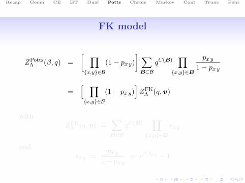
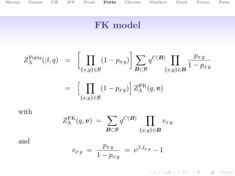
ZPottsΛ (β, q) =
[ ∏x,y∈B
(1− px y)] ∑
B⊂BqC(B)
∏x,y∈B
px y
1− px y
=[ ∏x,y∈B
(1− px y)]ZFK
Λ (q,v)
withZFK
Λ (q,v) =∑B⊂B
qC(B)∏
x,y∈B
vx y
andvx y =
px y
1− px y= eβ Jx y − 1
Recap Geom CE HT Dual Potts Chrom Markov Cont Trunc Penr
FK model
ZPottsΛ (β, q) =
[ ∏x,y∈B
(1− px y)] ∑
B⊂BqC(B)
∏x,y∈B
px y
1− px y
=[ ∏x,y∈B
(1− px y)]ZFK
Λ (q,v)
withZFK
Λ (q,v) =∑B⊂B
qC(B)∏
x,y∈B
vx y
andvx y =
px y
1− px y= eβ Jx y − 1
Recap Geom CE HT Dual Potts Chrom Markov Cont Trunc Penr
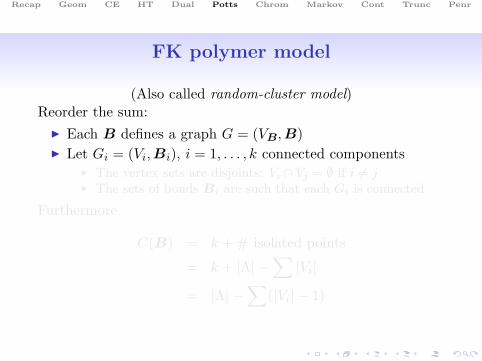
FK polymer model
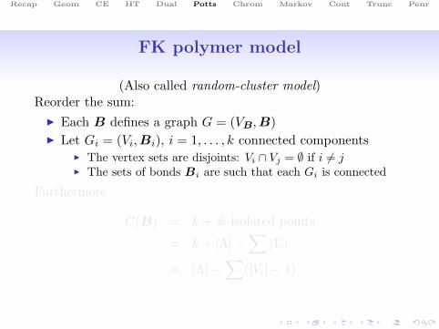
(Also called random-cluster model)Reorder the sum:
I Each B defines a graph G = (VB,B)I Let Gi = (Vi,Bi), i = 1, . . . , k connected components
I The vertex sets are disjoints: Vi ∩ Vj = ∅ if i 6= jI The sets of bonds Bi are such that each Gi is connected
Furthermore
C(B) = k + # isolated points
= k + |Λ| −∑
|Vi|
= |Λ| −∑
(|Vi| − 1)
Recap Geom CE HT Dual Potts Chrom Markov Cont Trunc Penr
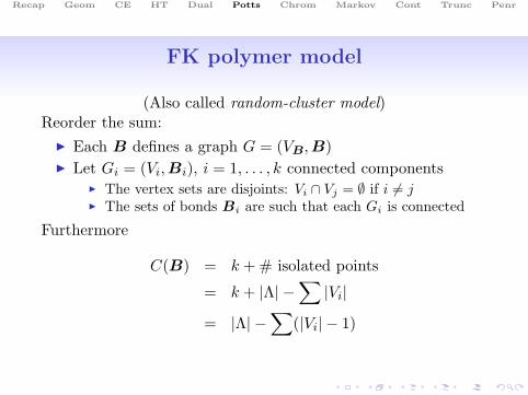
FK polymer model
(Also called random-cluster model)Reorder the sum:
I Each B defines a graph G = (VB,B)I Let Gi = (Vi,Bi), i = 1, . . . , k connected components
I The vertex sets are disjoints: Vi ∩ Vj = ∅ if i 6= jI The sets of bonds Bi are such that each Gi is connected
Furthermore
C(B) = k + # isolated points
= k + |Λ| −∑
|Vi|
= |Λ| −∑
(|Vi| − 1)
Recap Geom CE HT Dual Potts Chrom Markov Cont Trunc Penr
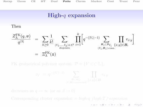
High-q expansion
Then
ZFKΛ (q,v)q|Λ|
=∑k≥0
1k!
∑(V1,...,Vk)∈Λk
disjoints
k∏i=1
[q−(|Vi|−1)
∑Bi⊂BVi
(Vi,Bi) conn.
∏x,y∈Bi
vx y
]
= ΞFKΛ (z)
FK geometrical polymer system: P = V ⊂⊂ L,
zV = q−(|V |−1)∑
B⊂BV(V,B) connected
∏x,y∈B
vx y
decreases as q →∞ (or as β → 0)
Corresponding cluster expansion = high-q (high-T ) expansion
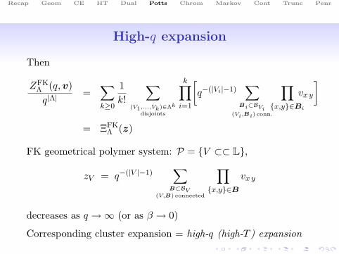
Recap Geom CE HT Dual Potts Chrom Markov Cont Trunc Penr
Chromatic polynomials
Given a graph G =(V (G), E(G)
):
PG(q) = # ways of properly coloring G with q colors
“properly” = adjacents vertices have different colors
If ω : V (G) → 1, . . . , q denote colorings
PG(q) =∑ω
∏x,y∈E(G)
[1− δωx ωy
]Introduced by Birkhoff (1912) to determine
χG = minq : PG(q) > 0
chromatic number = minimal q for a proper coloring
Recap Geom CE HT Dual Potts Chrom Markov Cont Trunc Penr
Tutte polynomial
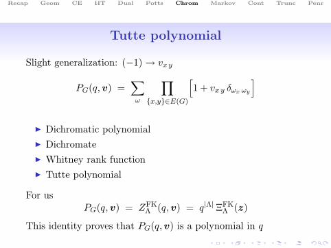
Slight generalization: (−1) → vx y
PG(q,v) =∑ω
∏x,y∈E(G)
[1 + vx y δωx ωy
]
I Dichromatic polynomialI DichromateI Whitney rank functionI Tutte polynomial
For usPG(q,v) = ZFK
Λ (q,v) = q|Λ| ΞFKΛ (z)
This identity proves that PG(q,v) is a polynomial in q
Recap Geom CE HT Dual Potts Chrom Markov Cont Trunc Penr
Tutte polynomial
Slight generalization: (−1) → vx y
PG(q,v) =∑ω
∏x,y∈E(G)
[1 + vx y δωx ωy
]
I Dichromatic polynomialI DichromateI Whitney rank functionI Tutte polynomial
For usPG(q,v) = ZFK
Λ (q,v) = q|Λ| ΞFKΛ (z)
This identity proves that PG(q,v) is a polynomial in q
Recap Geom CE HT Dual Potts Chrom Markov Cont Trunc Penr
Chromatic numbers and cluster expansions
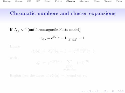
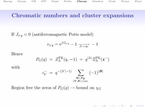
If Jx y < 0 (antiferromagnetic Potts model)
vx y = eβJx y − 1 −−−→β→∞ − 1
HencePG(q) = ZFK
Λ (q,−1) = q|Λ| ΞFKΛ (z−)
withz−V = q−(|V |−1)
∑B⊂BV
(V,B) conn.
(−1)|B|
Region free the zeros of PG(q) → bound on χG
Recap Geom CE HT Dual Potts Chrom Markov Cont Trunc Penr
Chromatic numbers and cluster expansions
If Jx y < 0 (antiferromagnetic Potts model)
vx y = eβJx y − 1 −−−→β→∞ − 1
HencePG(q) = ZFK
Λ (q,−1) = q|Λ| ΞFKΛ (z−)
withz−V = q−(|V |−1)
∑B⊂BV
(V,B) conn.
(−1)|B|
Region free the zeros of PG(q) → bound on χG
Recap Geom CE HT Dual Potts Chrom Markov Cont Trunc Penr
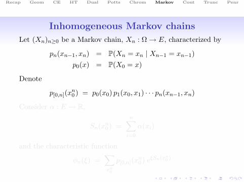
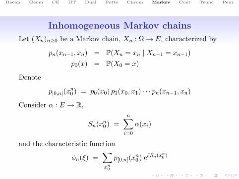
Inhomogeneous Markov chains
Let (Xn)n≥0 be a Markov chain, Xn : Ω → E, characterized by
pn(xn−1, xn) = P(Xn = xn | Xn−1 = xn−1)p0(x) = P(X0 = x)
Denote
p[0,n](xn0 ) = p0(x0) p1(x0, x1) · · · pn(xn−1, xn)
Consider α : E → R,
Sn(xn0 ) =
n∑i=0
α(xi)
and the characteristic function
φn(ξ) =∑xn0
p[0,n](xn0 ) eξSn(xn
0 )
Recap Geom CE HT Dual Potts Chrom Markov Cont Trunc Penr
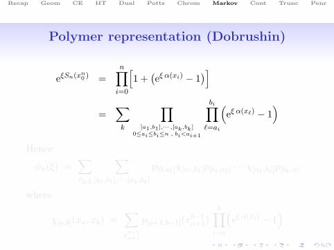
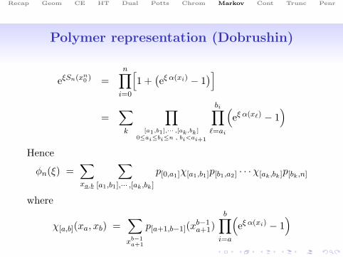
Polymer representation (Dobrushin)
eξSn(xn0 ) =
n∏i=0
[1 +
(eξ α(xi) − 1
)]=
∑k
∏[a1,b1],··· ,[ak,bk]
0≤ai≤bi≤n , bi<ai+1
bi∏`=ai
(eξ α(x`) − 1
)Hence
φn(ξ) =∑xa,b
∑[a1,b1],··· ,[ak,bk]
p[0,a1]χ[a1,b1]p[b1,a2] · · ·χ[ak,bk]p[bk,n]
where
χ[a,b](xa, xb) =∑xb−1
a+1
p[a+1,b−1](xb−1a+1)
b∏i=a
(eξ α(xi) − 1
)
Recap Geom CE HT Dual Potts Chrom Markov Cont Trunc Penr
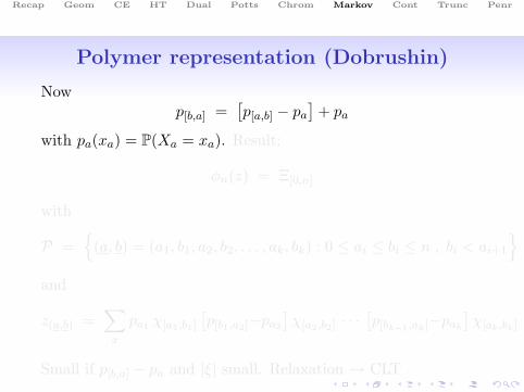
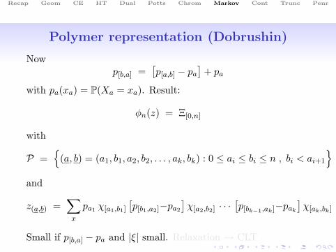
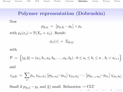
Polymer representation (Dobrushin)
Nowp[b,a] =
[p[a,b] − pa
]+ pa
with pa(xa) = P(Xa = xa). Result:
φn(z) = Ξ[0,n]
with
P =
(a, b) = (a1, b1, a2, b2, . . . , ak, bk) : 0 ≤ ai ≤ bi ≤ n , bi < ai+1
and
z(a,b) =∑
x
pa1 χ[a1,b1]
[p[b1,a2]−pa2
]χ[a2,b2] · · ·
[p[bk−1,ak]−pak
]χ[ak,bk]
Small if p[b,a] − pa and |ξ| small. Relaxation → CLT
Recap Geom CE HT Dual Potts Chrom Markov Cont Trunc Penr
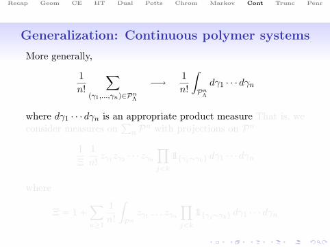
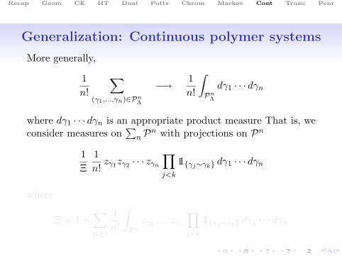
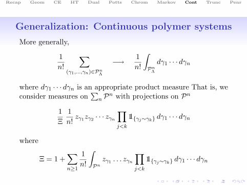
Generalization: Continuous polymer systems
More generally,
1n!
∑(γ1,...,γn)∈Pn
Λ
−→ 1n!
∫Pn
Λ
dγ1 · · · dγn
where dγ1 · · · dγn is an appropriate product measure That is, weconsider measures on
∑n Pn with projections on Pn
1Ξ
1n!zγ1zγ2 · · · zγn
∏j<k
11γj∼γk dγ1 · · · dγn
where
Ξ = 1 +∑n≥1
1n!
∫Pn
zγ1 . . . zγn
∏j<k
11γj∼γk dγ1 · · · dγn
Recap Geom CE HT Dual Potts Chrom Markov Cont Trunc Penr
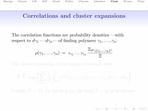
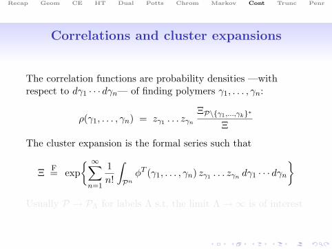
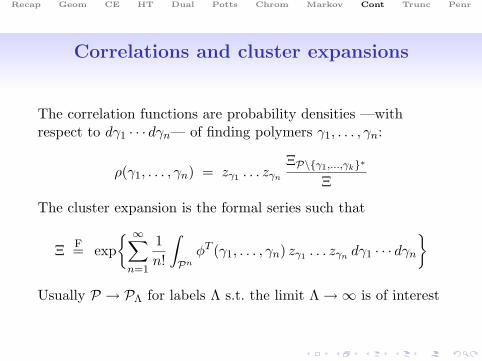
Correlations and cluster expansions
The correlation functions are probability densities —withrespect to dγ1 · · · dγn— of finding polymers γ1, . . . , γn:
ρ(γ1, . . . , γn) = zγ1 . . . zγn
ΞP\γ1,...,γk∗
Ξ
The cluster expansion is the formal series such that
Ξ F= exp ∞∑
n=1
1n!
∫Pn
φT (γ1, . . . , γn) zγ1 . . . zγn dγ1 · · · dγn
Usually P → PΛ for labels Λ s.t. the limit Λ →∞ is of interest
Recap Geom CE HT Dual Potts Chrom Markov Cont Trunc Penr
Correlations and cluster expansions
The correlation functions are probability densities —withrespect to dγ1 · · · dγn— of finding polymers γ1, . . . , γn:
ρ(γ1, . . . , γn) = zγ1 . . . zγn
ΞP\γ1,...,γk∗
Ξ
The cluster expansion is the formal series such that
Ξ F= exp ∞∑
n=1
1n!
∫Pn
φT (γ1, . . . , γn) zγ1 . . . zγn dγ1 · · · dγn
Usually P → PΛ for labels Λ s.t. the limit Λ →∞ is of interest

Recap Geom CE HT Dual Potts Chrom Markov Cont Trunc Penr
Example: Classical continuous gas
Basic setting
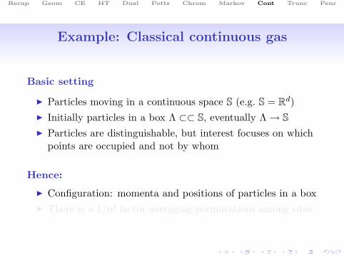
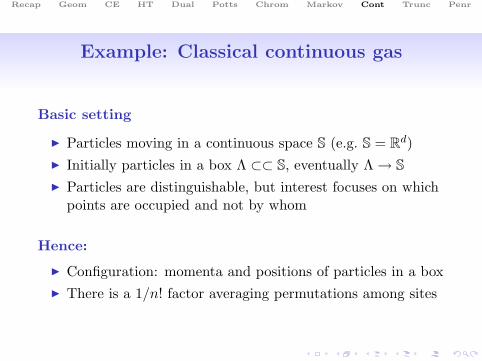
I Particles moving in a continuous space S (e.g. S = Rd)I Initially particles in a box Λ ⊂⊂ S, eventually Λ → SI Particles are distinguishable, but interest focuses on which
points are occupied and not by whom
Hence:
I Configuration: momenta and positions of particles in a boxI There is a 1/n! factor averaging permutations among sites

Recap Geom CE HT Dual Potts Chrom Markov Cont Trunc Penr
Example: Classical continuous gas
Basic setting
I Particles moving in a continuous space S (e.g. S = Rd)I Initially particles in a box Λ ⊂⊂ S, eventually Λ → SI Particles are distinguishable, but interest focuses on which
points are occupied and not by whom
Hence:
I Configuration: momenta and positions of particles in a boxI There is a 1/n! factor averaging permutations among sites
Recap Geom CE HT Dual Potts Chrom Markov Cont Trunc Penr
Ingredients of a continuous systems
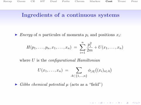
I Energy of n particules of momenta pi and positions xi:
H(p1, . . . , pn, x1, . . . , xn) =n∑
i=1
p2i
2m+ U(x1, . . . , xn)
where U is the configurational Hamiltonian
U(x1, . . . , xn) =∑
A⊂1,...,n
φ|A|((xi)i∈A
)I Gibbs chemical potential µ (acts as a “field”)
Recap Geom CE HT Dual Potts Chrom Markov Cont Trunc Penr
Grand canonical ensemble
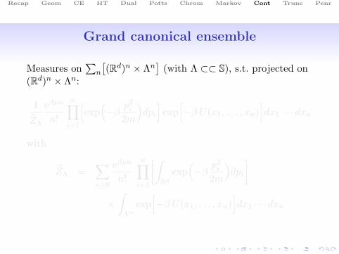
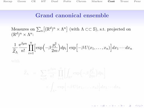
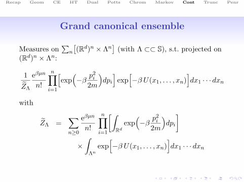
Measures on∑
n
[(Rd)n × Λn
](with Λ ⊂⊂ S), s.t. projected on
(Rd)n × Λn:
1
ZΛ
eβµn
n!
n∏i=1
[exp
(−β p
2i
2m
)dpi
]exp
[−β U(x1, . . . , xn)
]dx1 · · · dxn
with
ZΛ =∑n≥0
eβµn
n!
n∏i=1
[∫Rd
exp(−β p
2i
2m
)dpi
]×
∫Λn
exp[−β U(x1, . . . , xn)
]dx1 · · · dxn
Recap Geom CE HT Dual Potts Chrom Markov Cont Trunc Penr
Grand canonical ensemble
Measures on∑
n
[(Rd)n × Λn
](with Λ ⊂⊂ S), s.t. projected on
(Rd)n × Λn:
1
ZΛ
eβµn
n!
n∏i=1
[exp
(−β p
2i
2m
)dpi
]exp
[−β U(x1, . . . , xn)
]dx1 · · · dxn
with
ZΛ =∑n≥0
eβµn
n!
n∏i=1
[∫Rd
exp(−β p
2i
2m
)dpi
]×
∫Λn
exp[−β U(x1, . . . , xn)
]dx1 · · · dxn
Recap Geom CE HT Dual Potts Chrom Markov Cont Trunc Penr
Configurational ensemble
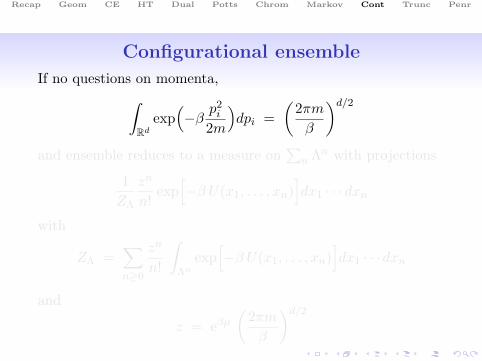
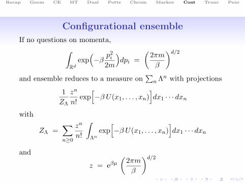
If no questions on momenta,∫Rd
exp(−β p
2i
2m
)dpi =
(2πmβ
)d/2
and ensemble reduces to a measure on∑
n Λn with projections
1ZΛ
zn
n!exp
[−β U(x1, . . . , xn)
]dx1 · · · dxn
with
ZΛ =∑n≥0
zn
n!
∫Λn
exp[−β U(x1, . . . , xn)
]dx1 · · · dxn
and
z = eβµ
(2πmβ
)d/2
Recap Geom CE HT Dual Potts Chrom Markov Cont Trunc Penr
Configurational ensemble
If no questions on momenta,∫Rd
exp(−β p
2i
2m
)dpi =
(2πmβ
)d/2
and ensemble reduces to a measure on∑
n Λn with projections
1ZΛ
zn
n!exp
[−β U(x1, . . . , xn)
]dx1 · · · dxn
with
ZΛ =∑n≥0
zn
n!
∫Λn
exp[−β U(x1, . . . , xn)
]dx1 · · · dxn
and
z = eβµ
(2πmβ
)d/2
Recap Geom CE HT Dual Potts Chrom Markov Cont Trunc Penr
Gas of hard spheres
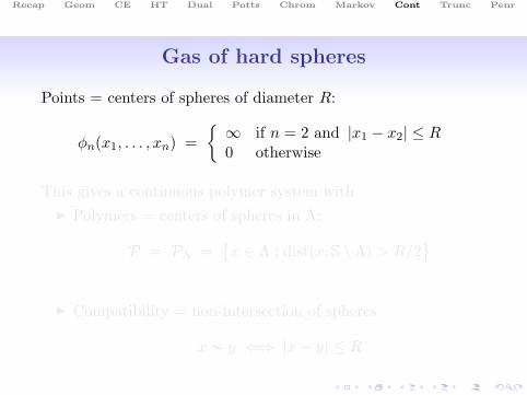
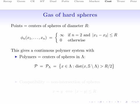
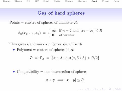
Points = centers of spheres of diameter R:
φn(x1, . . . , xn) =∞ if n = 2 and |x1 − x2| ≤ R0 otherwise
This gives a continuous polymer system withI Polymers = centers of spheres in Λ:
P = PΛ =x ∈ Λ : dist(x,S \ Λ) > R/2
I Compatibility = non-intersection of spheres
x y ⇐⇒ |x− y| ≤ R
Recap Geom CE HT Dual Potts Chrom Markov Cont Trunc Penr
Gas of hard spheres
Points = centers of spheres of diameter R:
φn(x1, . . . , xn) =∞ if n = 2 and |x1 − x2| ≤ R0 otherwise
This gives a continuous polymer system withI Polymers = centers of spheres in Λ:
P = PΛ =x ∈ Λ : dist(x,S \ Λ) > R/2
I Compatibility = non-intersection of spheres
x y ⇐⇒ |x− y| ≤ R
Recap Geom CE HT Dual Potts Chrom Markov Cont Trunc Penr
Cluster expansions - Classical strategy
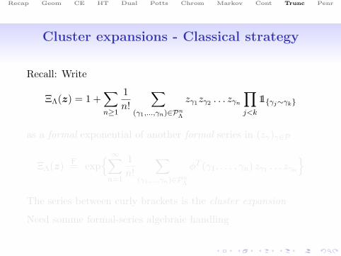
Recall: Write
ΞΛ(z) = 1 +∑n≥1
1n!
∑(γ1,...,γn)∈Pn
Λ
zγ1zγ2 . . . zγn
∏j<k
11γj∼γk
as a formal exponential of another formal series in (zγ)γ∈P
ΞΛ(z) F= exp ∞∑
n=1
1n!
∑(γ1,...,γn)∈Pn
Λ
φT (γ1, . . . , γn) zγ1 . . . zγn
The series between curly brackets is the cluster expansion
Need somme formal-series algebraic handling
Recap Geom CE HT Dual Potts Chrom Markov Cont Trunc Penr
Cluster expansions - Classical strategy
Recall: Write
ΞΛ(z) = 1 +∑n≥1
1n!
∑(γ1,...,γn)∈Pn
Λ
zγ1zγ2 . . . zγn
∏j<k
11γj∼γk
as a formal exponential of another formal series in (zγ)γ∈P
ΞΛ(z) F= exp ∞∑
n=1
1n!
∑(γ1,...,γn)∈Pn
Λ
φT (γ1, . . . , γn) zγ1 . . . zγn
The series between curly brackets is the cluster expansion
Need somme formal-series algebraic handling

Recap Geom CE HT Dual Potts Chrom Markov Cont Trunc Penr
Multiplicity functions
In general, we are dealing with series of the form
F (z) =∑n≥0
1n!
∑(γ1,...,γn)∈Pn
a(γ1, . . . , γn) zγ1 · · · zγn
Let us not assume anything about the coefficients other than
a(γ1, . . . , γn) is symmetric under permutations of (γ1, . . . , γn)
Therefore, a(γ1, . . . , γn) is a fcn. of the multiplicty function:
M : P(N) −→ N(P)[M(γ1, . . . , γn)
]γ
= #i : γi = γ
Recap Geom CE HT Dual Potts Chrom Markov Cont Trunc Penr
Exponential generating functions
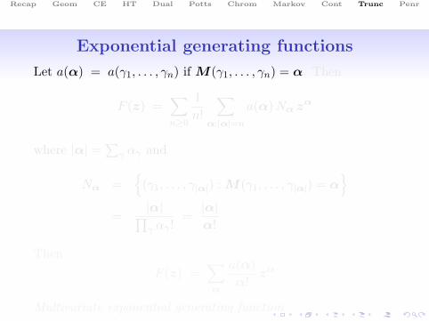
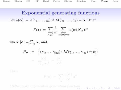
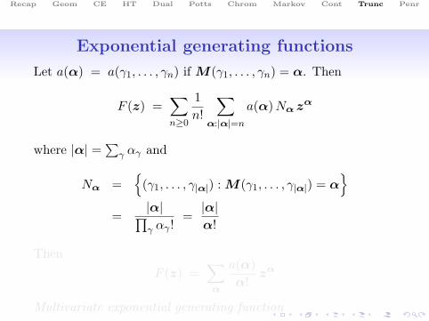
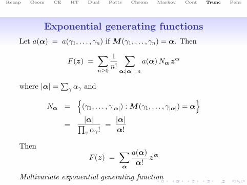
Let a(α) = a(γ1, . . . , γn) if M(γ1, . . . , γn) = α. Then
F (z) =∑n≥0
1n!
∑α:|α|=n
a(α)Nα zα
where |α| =∑
γ αγ and
Nα =
(γ1, . . . , γ|α|) : M(γ1, . . . , γ|α|) = α
=|α|∏γ αγ !
=|α|α!
ThenF (z) =
∑α
a(α)α!
zα
Multivariate exponential generating function
Recap Geom CE HT Dual Potts Chrom Markov Cont Trunc Penr
Exponential generating functions
Let a(α) = a(γ1, . . . , γn) if M(γ1, . . . , γn) = α. Then
F (z) =∑n≥0
1n!
∑α:|α|=n
a(α)Nα zα
where |α| =∑
γ αγ and
Nα =
(γ1, . . . , γ|α|) : M(γ1, . . . , γ|α|) = α
=|α|∏γ αγ !
=|α|α!
ThenF (z) =
∑α
a(α)α!
zα
Multivariate exponential generating function
Recap Geom CE HT Dual Potts Chrom Markov Cont Trunc Penr
The truncated coefficients
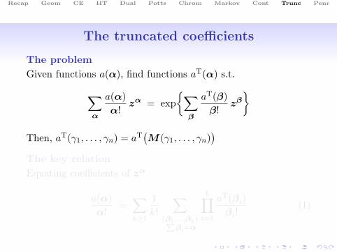
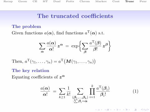
The problemGiven functions a(α), find functions aT(α) s.t.
∑α
a(α)α!
zα = exp∑
β
aT(β)β!
zβ
Then, aT(γ1, . . . , γn) = aT(M(γ1, . . . , γn)
)The key relationEquating coefficients of zα
a(α)α!
=∑k≥1
1k!
∑(β1,...,βk):P
βi=α
k∏i=1
aT(βi)βi!
(1)
Recap Geom CE HT Dual Potts Chrom Markov Cont Trunc Penr
The truncated coefficients
The problemGiven functions a(α), find functions aT(α) s.t.
∑α
a(α)α!
zα = exp∑
β
aT(β)β!
zβ
Then, aT(γ1, . . . , γn) = aT(M(γ1, . . . , γn)
)The key relationEquating coefficients of zα
a(α)α!
=∑k≥1
1k!
∑(β1,...,βk):P
βi=α
k∏i=1
aT(βi)βi!
(1)

Recap Geom CE HT Dual Potts Chrom Markov Cont Trunc Penr
Algebraic facts
Key observation 1:Previous expression uniquely determines aT:
|α| = 1 a(γ) = aT(γ)|α| = 2 a(γ1, γ2) = aT(γ1, γ2) + aT(γ1) aT(γ2)
= aT(γ1, γ2) + a(γ1) a(γ2)|α| = n . . . (induction)
Key observation 2:Better to go back to n-tuples
a(γ1, . . . , γn) = α!∑k≥1
1k!
∑(β1,...,βk):P
βi=α
k∏i=1
aT(γIi)βi!
I1, . . . , Ik partition of 1, . . . , n (subseqs.) s.t. βi = M(γIi)
Recap Geom CE HT Dual Potts Chrom Markov Cont Trunc Penr
Number of partitions
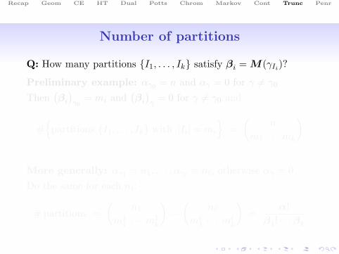
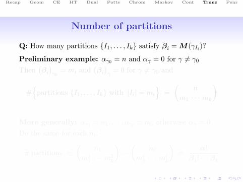
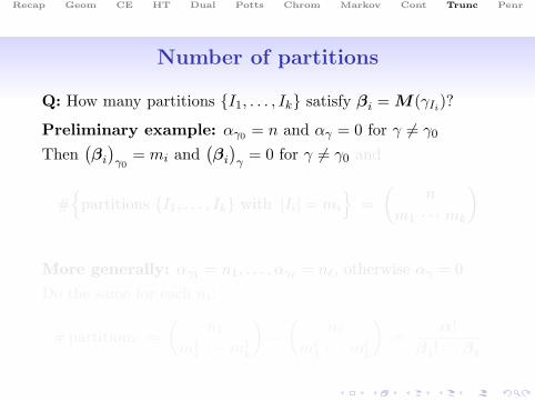
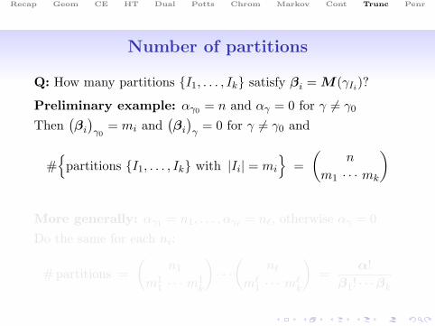
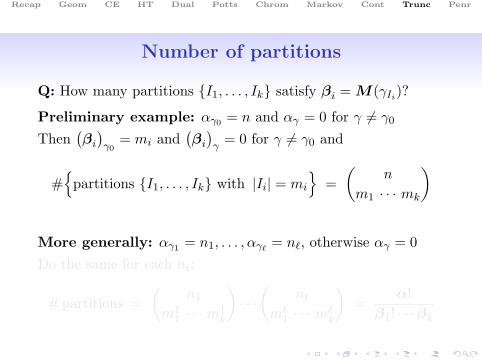
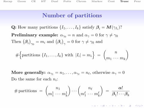
Q: How many partitions I1, . . . , Ik satisfy βi = M(γIi)?
Preliminary example: αγ0 = n and αγ = 0 for γ 6= γ0
Then(βi
)γ0
= mi and(βi
)γ
= 0 for γ 6= γ0 and
#
partitions I1, . . . , Ik with |Ii| = mi
=
(n
m1 · · · mk
)
More generally: αγ1 = n1, . . . , αγ`= n`, otherwise αγ = 0
Do the same for each ni:
# partitions =(
n1
m11 · · · m1
k
)· · ·
(n`
m`1 · · · m`
k
)=
α!β1! · · ·βk
Recap Geom CE HT Dual Potts Chrom Markov Cont Trunc Penr
Number of partitions
Q: How many partitions I1, . . . , Ik satisfy βi = M(γIi)?
Preliminary example: αγ0 = n and αγ = 0 for γ 6= γ0
Then(βi
)γ0
= mi and(βi
)γ
= 0 for γ 6= γ0 and
#
partitions I1, . . . , Ik with |Ii| = mi
=
(n
m1 · · · mk
)
More generally: αγ1 = n1, . . . , αγ`= n`, otherwise αγ = 0
Do the same for each ni:
# partitions =(
n1
m11 · · · m1
k
)· · ·
(n`
m`1 · · · m`
k
)=
α!β1! · · ·βk
Recap Geom CE HT Dual Potts Chrom Markov Cont Trunc Penr
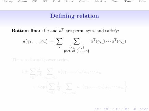
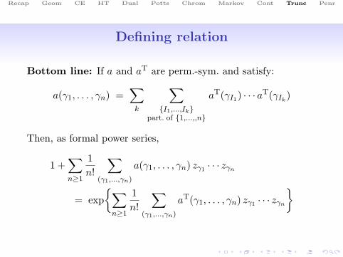
Defining relation
Bottom line: If a and aT are perm.-sym. and satisfy:
a(γ1, . . . , γn) =∑
k
∑I1,...,Ik
part. of 1,...,,n
aT(γI1) · · · aT(γIk)
Then, as formal power series,
1 +∑n≥1
1n!
∑(γ1,...,γn)
a(γ1, . . . , γn) zγ1 · · · zγn
= exp∑
n≥1
1n!
∑(γ1,...,γn)
aT(γ1, . . . , γn) zγ1 · · · zγn
Recap Geom CE HT Dual Potts Chrom Markov Cont Trunc Penr
Defining relation
Bottom line: If a and aT are perm.-sym. and satisfy:
a(γ1, . . . , γn) =∑
k
∑I1,...,Ik
part. of 1,...,,n
aT(γI1) · · · aT(γIk)
Then, as formal power series,
1 +∑n≥1
1n!
∑(γ1,...,γn)
a(γ1, . . . , γn) zγ1 · · · zγn
= exp∑
n≥1
1n!
∑(γ1,...,γn)
aT(γ1, . . . , γn) zγ1 · · · zγn

Recap Geom CE HT Dual Potts Chrom Markov Cont Trunc Penr
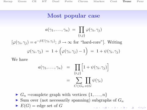
Most popular case
a(γ1, . . . , γn) =∏i,j
ϕ(γi, γj)
[ϕ(γi, γj) = e−β U(γ1,γj); β →∞ for “hard-core”]. Writing
ϕ(γi, γj) = 1 +(ϕ(γi, γj)− 1
)= 1 + ψ(γi, γj)
We have
a(γ1, . . . , γn) =∏i,j
[1 + ψ(γi, γj)
]=
∑C⊂Gn
∏e∈G
ψ(γe)
I Gn =complete graph with vertices 1, . . . , nI Sum over (not necessarily spanning) subgraphs of Gn
I E(G) = edge set of G

Recap Geom CE HT Dual Potts Chrom Markov Cont Trunc Penr
Most popular case
a(γ1, . . . , γn) =∏i,j
ϕ(γi, γj)
[ϕ(γi, γj) = e−β U(γ1,γj); β →∞ for “hard-core”]. Writing
ϕ(γi, γj) = 1 +(ϕ(γi, γj)− 1
)= 1 + ψ(γi, γj)
We have
a(γ1, . . . , γn) =∏i,j
[1 + ψ(γi, γj)
]=
∑C⊂Gn
∏e∈G
ψ(γe)
I Gn =complete graph with vertices 1, . . . , nI Sum over (not necessarily spanning) subgraphs of Gn
I E(G) = edge set of G
Recap Geom CE HT Dual Potts Chrom Markov Cont Trunc Penr
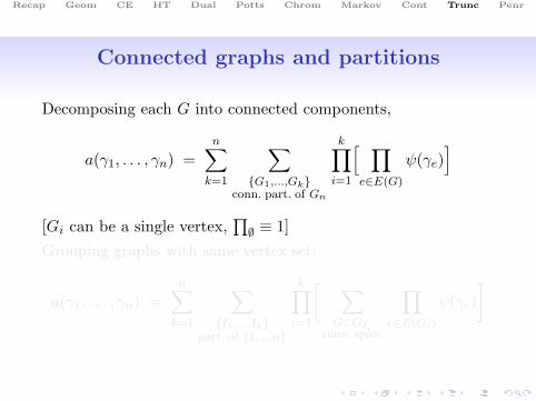
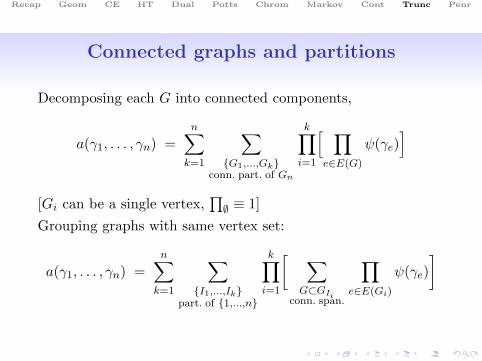
Connected graphs and partitions
Decomposing each G into connected components,
a(γ1, . . . , γn) =n∑
k=1
∑G1,...,Gk
conn. part. of Gn
k∏i=1
[ ∏e∈E(G)
ψ(γe)]
[Gi can be a single vertex,∏∅ ≡ 1]
Grouping graphs with same vertex set:
a(γ1, . . . , γn) =n∑
k=1
∑I1,...,Ik
part. of 1,...,n
k∏i=1
[ ∑G⊂GIi
conn. span.
∏e∈E(Gi)
ψ(γe)]
Recap Geom CE HT Dual Potts Chrom Markov Cont Trunc Penr
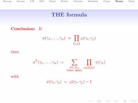
THE formula
Conclusion: If
a(γ1, . . . , γn) =∏i,j
ϕ(γi, γj)
then
aT(γ1, . . . , γn) =∑
G⊂Gnconn. span.
∏e∈E(G)
ψ(γe)
withψ(γi, γj) = ϕ(γi, γj)− 1

Recap Geom CE HT Dual Potts Chrom Markov Cont Trunc Penr
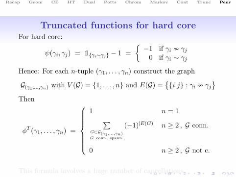
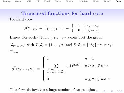
Truncated functions for hard coreFor hard core:
ψ(γi, γj) = 11γi∼γj − 1 =−1 if γi γj
0 if γi ∼ γj
Hence: For each n-tuple (γ1, . . . , γn) construct the graph
G(γ1,...,γn) with V (G) = 1, . . . , n and E(G) =i.j : γi γj
Then
φT (γ1, . . . , γn) =
1 n = 1∑G⊂G(γ1,...,γn)G conn. spann.
(−1)|E(G)| n ≥ 2 , G conn.
0 n ≥ 2 , G not c.
This formula involves a huge number of cancellations

Recap Geom CE HT Dual Potts Chrom Markov Cont Trunc Penr
Truncated functions for hard coreFor hard core:
ψ(γi, γj) = 11γi∼γj − 1 =−1 if γi γj
0 if γi ∼ γj
Hence: For each n-tuple (γ1, . . . , γn) construct the graph
G(γ1,...,γn) with V (G) = 1, . . . , n and E(G) =i.j : γi γj
Then
φT (γ1, . . . , γn) =
1 n = 1∑G⊂G(γ1,...,γn)G conn. spann.
(−1)|E(G)| n ≥ 2 , G conn.
0 n ≥ 2 , G not c.
This formula involves a huge number of cancellations

Recap Geom CE HT Dual Potts Chrom Markov Cont Trunc Penr
Penrose identity
Penrose realized that these cancellations can be optimallyhandled through what is now known as the property ofpartitionability of the family of connected spanning subgraphs
TheoremFor any connected graph G = (V,E) there exists a family ofspanning trees —the Penrose trees T Penr
G — such that∑G⊂G
(−1)|E(G)| = (−1)|V|−1∣∣T PenrG
∣∣

Recap Geom CE HT Dual Potts Chrom Markov Cont Trunc Penr
Partitionability of subgraphs
LetI G = (U,E) a finite connected graphI CG = connected spanning subgraphs of GI TG = trees belonging to CG
Partial-order CG by bond inclusion:
G ≤ G ⇐⇒ E(G) ⊂ E(G)
If G ≤ G, let
[G, G] = G ∈ CG : G ≤ G ≤ G

Recap Geom CE HT Dual Potts Chrom Markov Cont Trunc Penr
Partitionability of subgraphs
LetI G = (U,E) a finite connected graphI CG = connected spanning subgraphs of GI TG = trees belonging to CG
Partial-order CG by bond inclusion:
G ≤ G ⇐⇒ E(G) ⊂ E(G)
If G ≤ G, let
[G, G] = G ∈ CG : G ≤ G ≤ G

Recap Geom CE HT Dual Potts Chrom Markov Cont Trunc Penr
Partitionability of subgraphs
LetI G = (U,E) a finite connected graphI CG = connected spanning subgraphs of GI TG = trees belonging to CG
Partial-order CG by bond inclusion:
G ≤ G ⇐⇒ E(G) ⊂ E(G)
If G ≤ G, let
[G, G] = G ∈ CG : G ≤ G ≤ G

Recap Geom CE HT Dual Potts Chrom Markov Cont Trunc Penr
Partition schemes
A partition scheme for CG is a map
R : TG −→ CGτ 7−→ R(τ)
such that(i) E
(R(τ)
)⊃ E(τ), and
(ii) CG is the disjoint union of the sets [τ,R(τ)], τ ∈ TG.
Recap Geom CE HT Dual Potts Chrom Markov Cont Trunc Penr
Partition schemes
A partition scheme for CG is a map
R : TG −→ CGτ 7−→ R(τ)
such that(i) E
(R(τ)
)⊃ E(τ), and
(ii) CG is the disjoint union of the sets [τ,R(τ)], τ ∈ TG.
Recap Geom CE HT Dual Potts Chrom Markov Cont Trunc Penr
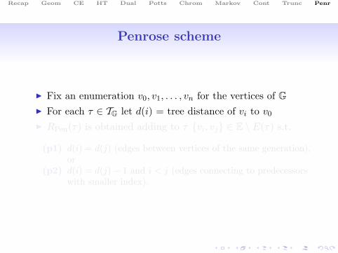
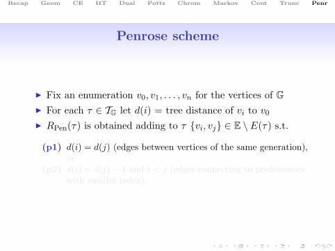
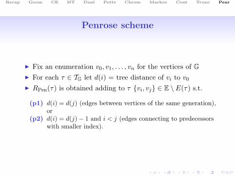
Penrose scheme
I Fix an enumeration v0, v1, . . . , vn for the vertices of GI For each τ ∈ TG let d(i) = tree distance of vi to v0I RPen(τ) is obtained adding to τ vi, vj ∈ E \ E(τ) s.t.
(p1) d(i) = d(j) (edges between vertices of the same generation),or
(p2) d(i) = d(j)− 1 and i < j (edges connecting to predecessorswith smaller index).
Recap Geom CE HT Dual Potts Chrom Markov Cont Trunc Penr
Penrose identity
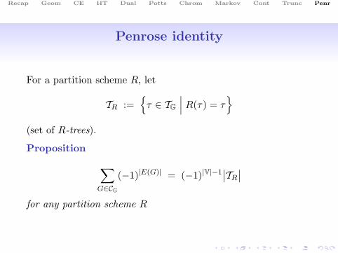
For a partition scheme R, let
TR :=τ ∈ TG
∣∣∣ R(τ) = τ
(set of R-trees).
Proposition ∑G∈CG
(−1)|E(G)| = (−1)|V|−1∣∣TR
∣∣for any partition scheme R
Recap Geom CE HT Dual Potts Chrom Markov Cont Trunc Penr
Proof of Penrose identity
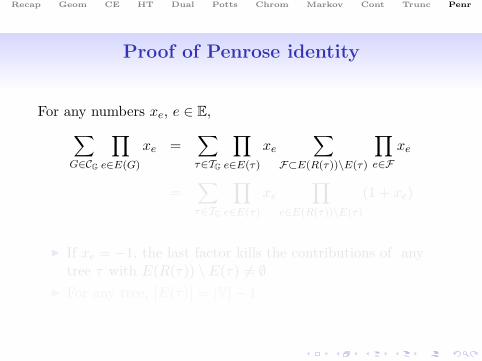
For any numbers xe, e ∈ E,∑G∈CG
∏e∈E(G)
xe =∑τ∈TG
∏e∈E(τ)
xe
∑F⊂E(R(τ))\E(τ)
∏e∈F
xe
=∑τ∈TG
∏e∈E(τ)
xe
∏e∈E(R(τ))\E(τ)
(1 + xe)
I If xe = −1, the last factor kills the contributions of anytree τ with E(R(τ)) \ E(τ) 6= ∅
I For any tree,∣∣E(τ)
∣∣ = |V| − 1
Recap Geom CE HT Dual Potts Chrom Markov Cont Trunc Penr
Proof of Penrose identity
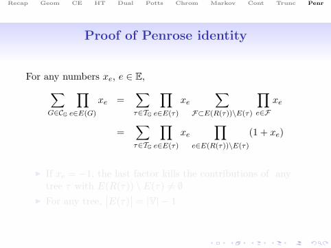
For any numbers xe, e ∈ E,∑G∈CG
∏e∈E(G)
xe =∑τ∈TG
∏e∈E(τ)
xe
∑F⊂E(R(τ))\E(τ)
∏e∈F
xe
=∑τ∈TG
∏e∈E(τ)
xe
∏e∈E(R(τ))\E(τ)
(1 + xe)
I If xe = −1, the last factor kills the contributions of anytree τ with E(R(τ)) \ E(τ) 6= ∅
I For any tree,∣∣E(τ)
∣∣ = |V| − 1

Recap Geom CE HT Dual Potts Chrom Markov Cont Trunc Penr
Proof of Penrose identity
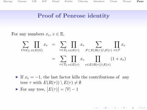
For any numbers xe, e ∈ E,∑G∈CG
∏e∈E(G)
xe =∑τ∈TG
∏e∈E(τ)
xe
∑F⊂E(R(τ))\E(τ)
∏e∈F
xe
=∑τ∈TG
∏e∈E(τ)
xe
∏e∈E(R(τ))\E(τ)
(1 + xe)
I If xe = −1, the last factor kills the contributions of anytree τ with E(R(τ)) \ E(τ) 6= ∅
I For any tree,∣∣E(τ)
∣∣ = |V| − 1
Recap Geom CE HT Dual Potts Chrom Markov Cont Trunc Penr
Proof of Penrose identity
For any numbers xe, e ∈ E,∑G∈CG
∏e∈E(G)
xe =∑τ∈TG
∏e∈E(τ)
xe
∑F⊂E(R(τ))\E(τ)
∏e∈F
xe
=∑τ∈TG
∏e∈E(τ)
xe
∏e∈E(R(τ))\E(τ)
(1 + xe)
I If xe = −1, the last factor kills the contributions of anytree τ with E(R(τ)) \ E(τ) 6= ∅
I For any tree,∣∣E(τ)
∣∣ = |V| − 1
Recap Geom CE HT Dual Potts Chrom Markov Cont Trunc Penr
Comments
I Hard-core condition is crucial. If only soft repulsion,
|1 + xe| ≤ 1
and we get the weaker tree-graph bound∣∣∣ ∑G∈CG
∏e∈E(G)
xe
∣∣∣ ≤ ∑τ∈TG
∏e∈E(τ)
|xe| ≤ |TG|
I The smaller the number of triangle diagrams, the larger thenumber of Penrose trees. Hence:
R(G) ⊃ R(tree with larger degrees)⊃ R(homogeneous tree with max. degree)


![The Interaction Between Amphiphilic Polymer Materials and ...€¦ · guest molecules. [ 9 ] By tuning the interaction between the polymer materials and guest drugs, amphi-philic](https://static.fdocument.org/doc/165x107/60b7e318a87bed0fba1a5735/the-interaction-between-amphiphilic-polymer-materials-and-guest-molecules-.jpg)


![European Polymer Journal - web.itu.edu.tr · (HEMA) and N-vinylpyrrolidone (NVP) hydrogels to enhance the hy-drogels’ swelling and degradation properties [31]. Semi-degradable polymer](https://static.fdocument.org/doc/165x107/5d50e19a88c99350328b630d/european-polymer-journal-webituedutr-hema-and-n-vinylpyrrolidone-nvp.jpg)