Rates of convergence for approximations of viscosity ...
127
1 Rates of convergence for approximations of viscosity solutions and homogenization Panagiotis E. Souganidis The University of Texas at Austin Nonlinear approximation techniques using L 1 Texas A&M University May 2008
Transcript of Rates of convergence for approximations of viscosity ...
1
Rates of convergence for approximationsof viscosity solutions and homogenization
Panagiotis E. SouganidisThe University of Texas at Austin
Nonlinear approximation techniques usingL1
Texas A&M UniversityMay 2008
2
F(D2u, Du, u, x) = 0 in U
3
F(D2u, Du, u, x) = 0 in U
numerical approximations
monotone, stable, consistentapproximations
Fh(D2huh,Dhuh, uh, x) = 0 in Uh
uh → u and uh − u = O(σ(h))
mesh sizeh, numerical nonlinearityFh,solutionuh, domainUh = U ∩ Z
Nh
4
F(D2u, Du, u, x) = 0 in U
numerical approximations
monotone, stable, consistentapproximations
Fh(D2huh,Dhuh, uh, x) = 0 in Uh
uh → u and uh − u = O(σ(h))
mesh sizeh, numerical nonlinearityFh,solutionuh, domainUh = U ∩ Z
Nh
homogenization
F(D2uε,Duε, uε,xε, ω) = 0 in U F0(D2u0,Du0, u0) = 0 in U
uε → u0 and uε − u0 = O(σ(ε))
5
NUMERICAL APPROXIMATIONS
6
NUMERICAL APPROXIMATIONS
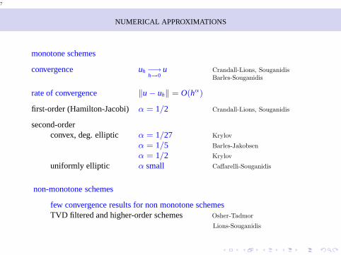
monotone schemes
convergence uh −→h→0
u Crandall-Lions, SouganidisBarles-Souganidis
rate of convergence ‖u − uh‖ = O(hα)
first-order (Hamilton-Jacobi) α = 1/2 Crandall-Lions, Souganidis
second-orderconvex, deg. elliptic α = 1/27 Krylov
α = 1/5 Barles-Jakobsen
α = 1/2 Krylov
uniformly elliptic α small Caffarelli-Souganidis
7
NUMERICAL APPROXIMATIONS
monotone schemes
convergence uh −→h→0
u Crandall-Lions, SouganidisBarles-Souganidis
rate of convergence ‖u − uh‖ = O(hα)
first-order (Hamilton-Jacobi) α = 1/2 Crandall-Lions, Souganidis
second-orderconvex, deg. elliptic α = 1/27 Krylov
α = 1/5 Barles-Jakobsen
α = 1/2 Krylov
uniformly elliptic α small Caffarelli-Souganidis
non-monotone schemes
few convergence results for non monotone schemesTVD filtered and higher-order schemes Osher-Tadmor
Lions-Souganidis
8
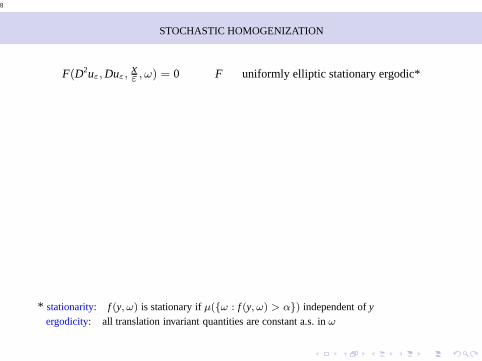
STOCHASTIC HOMOGENIZATION
F(D2uε,Duε,xε , ω) = 0 F uniformly elliptic stationary ergodic*
* stationarity: f (y, ω) is stationary ifµ(ω : f (y, ω) > α) independent ofyergodicity: all translation invariant quantities are constant a.s. inω
9
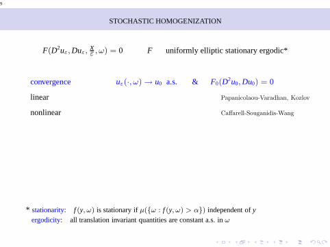
STOCHASTIC HOMOGENIZATION
F(D2uε,Duε,xε , ω) = 0 F uniformly elliptic stationary ergodic*
convergence uε(·, ω) → u0 a.s. & F0(D2u0,Du0) = 0
linear Papanicolaou-Varadhan, Kozlov
nonlinear Caffarell-Souganidis-Wang
* stationarity: f (y, ω) is stationary ifµ(ω : f (y, ω) > α) independent ofyergodicity: all translation invariant quantities are constant a.s. inω

10
STOCHASTIC HOMOGENIZATION
F(D2uε,Duε,xε , ω) = 0 F uniformly elliptic stationary ergodic*
convergence uε(·, ω) → u0 a.s. & F0(D2u0,Du0) = 0
linear Papanicolaou-Varadhan, Kozlov
nonlinear Caffarell-Souganidis-Wang
rates of convergence strongly mixing media with algebraic rate
linear ‖uε − u0‖ = O(εγ) a.s. Yurinskii
nonlinear ‖uε − u0‖ = O(e−c| ln ε|1/2) off
Caffarelli-Souganidisa set with probabilityO(e−c| ln ε|1/2
)
* stationarity: f (y, ω) is stationary ifµ(ω : f (y, ω) > α) independent ofyergodicity: all translation invariant quantities are constant a.s. inω
11
CONVERGENCE OF MONOTONE APPROXIMATIONS
(F) F(D2u,Du, u, x) = 0
12
CONVERGENCE OF MONOTONE APPROXIMATIONS
(F) F(D2u,Du, u, x) = 0
F degenerate elliptic (X ≦ Y =⇒ F(X, p, r, x) ≧ F(Y ,p, r, x))
13
CONVERGENCE OF MONOTONE APPROXIMATIONS
(F) F(D2u,Du, u, x) = 0
F degenerate elliptic (X ≦ Y =⇒ F(X, p, r, x) ≧ F(Y ,p, r, x))
approximation scheme S([uh]x, uh(x), x, h) = 0
14
CONVERGENCE OF MONOTONE APPROXIMATIONS
(F) F(D2u,Du, u, x) = 0
F degenerate elliptic (X ≦ Y =⇒ F(X, p, r, x) ≧ F(Y ,p, r, x))
approximation scheme S([uh]x, uh(x), x, h) = 0
monotone u ≥ v =⇒ S([u]x, s, x, h) ≦ S([v]x, s, x, h)
15
CONVERGENCE OF MONOTONE APPROXIMATIONS
(F) F(D2u,Du, u, x) = 0
F degenerate elliptic (X ≦ Y =⇒ F(X, p, r, x) ≧ F(Y ,p, r, x))
approximation scheme S([uh]x, uh(x), x, h) = 0
monotone u ≥ v =⇒ S([u]x, s, x, h) ≦ S([v]x, s, x, h)
stable ‖uh‖ ≦ C independent ofh
16
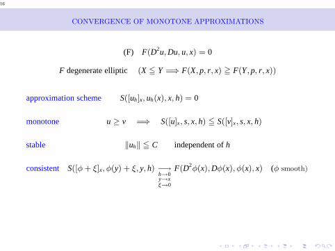
CONVERGENCE OF MONOTONE APPROXIMATIONS
(F) F(D2u,Du, u, x) = 0
F degenerate elliptic (X ≦ Y =⇒ F(X, p, r, x) ≧ F(Y ,p, r, x))
approximation scheme S([uh]x, uh(x), x, h) = 0
monotone u ≥ v =⇒ S([u]x, s, x, h) ≦ S([v]x, s, x, h)
stable ‖uh‖ ≦ C independent ofh
consistent S([φ+ ξ]x, φ(y) + ξ, y, h) −→h→0y→xξ→0
F(D2φ(x),Dφ(x), φ(x), x) (φ smooth)
17
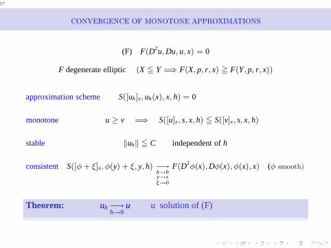
CONVERGENCE OF MONOTONE APPROXIMATIONS
(F) F(D2u,Du, u, x) = 0
F degenerate elliptic (X ≦ Y =⇒ F(X, p, r, x) ≧ F(Y ,p, r, x))
approximation scheme S([uh]x, uh(x), x, h) = 0
monotone u ≥ v =⇒ S([u]x, s, x, h) ≦ S([v]x, s, x, h)
stable ‖uh‖ ≦ C independent ofh
consistent S([φ+ ξ]x, φ(y) + ξ, y, h) −→h→0y→xξ→0
F(D2φ(x),Dφ(x), φ(x), x) (φ smooth)
Theorem: uh −→h→0
u u solution of (F)

18
Proof
19
Proof
S([uh]x, uh(x), x, h) = 0
20
Proof
S([uh]x, uh(x), x, h) = 0
stability =⇒
u∗(x) = limy→xh→0
uh(y)
u∗(x) = limy→0h→0
uh(y)exist
21
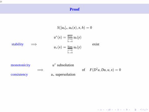
Proof
S([uh]x, uh(x), x, h) = 0
stability =⇒
u∗(x) = limy→xh→0
uh(y)
u∗(x) = limy→0h→0
uh(y)exist
monotonicity
consistency=⇒
u∗ subsolution
u∗ supersolutionof F(D2u,Du, u, x) = 0
22
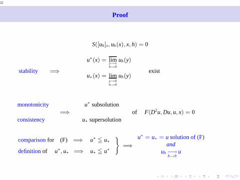
Proof
S([uh]x, uh(x), x, h) = 0
stability =⇒
u∗(x) = limy→xh→0
uh(y)
u∗(x) = limy→0h→0
uh(y)exist
monotonicity
consistency=⇒
u∗ subsolution
u∗ supersolutionof F(D2u,Du, u, x) = 0
comparisonfor (F) =⇒
definitionof u∗, u∗ =⇒
u∗ ≦ u∗
u∗ ≦ u∗
)
=⇒
u∗ = u∗ = u solution of (F)and
uh −→h→0
u
23
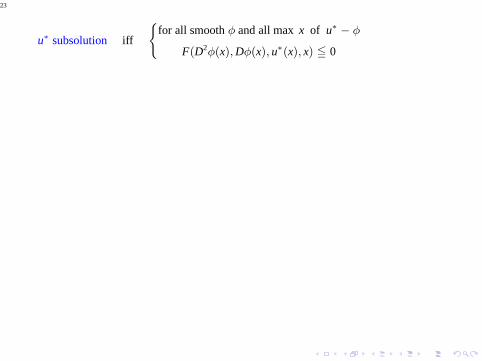
u∗ subsolution iff
(for all smoothφ and all maxx of u∗ − φ
F(D2φ(x),Dφ(x), u∗(x), x) ≦ 0
24
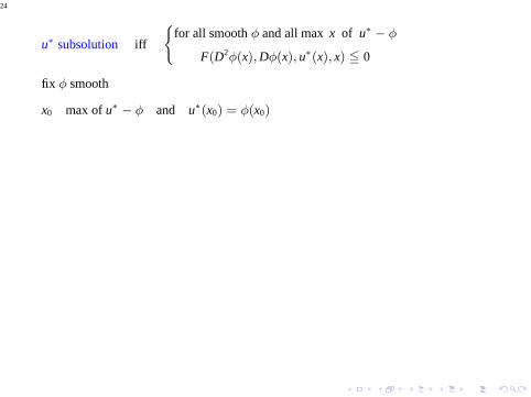
u∗ subsolution iff
(for all smoothφ and all maxx of u∗ − φ
F(D2φ(x),Dφ(x), u∗(x), x) ≦ 0
fix φ smooth
x0 max ofu∗ − φ and u∗(x0) = φ(x0)
25
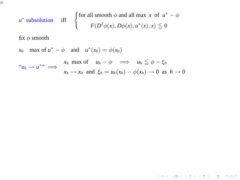
u∗ subsolution iff
(for all smoothφ and all maxx of u∗ − φ
F(D2φ(x),Dφ(x), u∗(x), x) ≦ 0
fix φ smooth
x0 max ofu∗ − φ and u∗(x0) = φ(x0)
“uh → u∗” =⇒xh max of uh − φ =⇒ uh ≦ φ− ξh
xh → x0 and ξh = uh(xh) − φ(xh) → 0 as h → 0
26
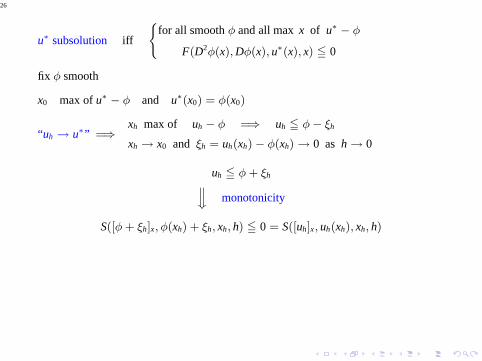
u∗ subsolution iff
(for all smoothφ and all maxx of u∗ − φ
F(D2φ(x),Dφ(x), u∗(x), x) ≦ 0
fix φ smooth
x0 max ofu∗ − φ and u∗(x0) = φ(x0)
“uh → u∗” =⇒xh max of uh − φ =⇒ uh ≦ φ− ξh
xh → x0 and ξh = uh(xh) − φ(xh) → 0 as h → 0
uh ≦ φ+ ξhww monotonicity
S([φ+ ξh]x, φ(xh) + ξh, xh, h) ≦ 0 = S([uh]x, uh(xh), xh, h)
27
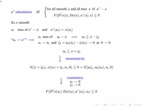
u∗ subsolution iff
(for all smoothφ and all maxx of u∗ − φ
F(D2φ(x),Dφ(x), u∗(x), x) ≦ 0
fix φ smooth
x0 max ofu∗ − φ and u∗(x0) = φ(x0)
“uh → u∗” =⇒xh max of uh − φ =⇒ uh ≦ φ− ξh
xh → x0 and ξh = uh(xh) − φ(xh) → 0 as h → 0
uh ≦ φ+ ξhww monotonicity
S([φ+ ξh]x, φ(xh) + ξh, xh, h) ≦ 0 = S([uh]x, uh(xh), xh, h)
ww
consistencyxh → 0ξh → 0
F(D2φ(x0),Dφ(x0), u∗(x0), x0) ≦ 0
28
Examples
• Hamilton-Jacobi equation ut + H(ux) = 0
29
Examples
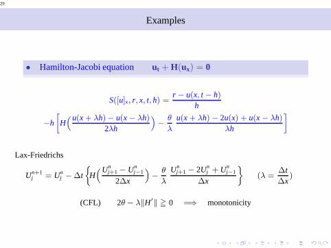
• Hamilton-Jacobi equation ut + H(ux) = 0
S([u]x, r, x, t, h) =r − u(x, t − h)
h
−h
»
H“u(x + λh) − u(x − λh)
2λh
”
−θ
λ
u(x + λh) − 2u(x) + u(x − λh)
λh
–
Lax-Friedrichs
Un+1j = Un
j − ∆t
H“Un
j+1 − Unj−1
2∆x
”
−θ
λ
Unj+1 − 2Un
j + Unj−1
∆x
ff
(λ =∆t∆x
)
(CFL) 2θ − λ‖H′‖ ≧ 0 =⇒ monotonicity
30
• Isaacs-Bellman equation ut + F(D2u, Du, x) = 0
31
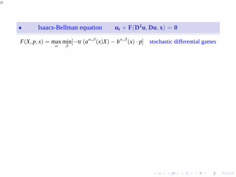
• Isaacs-Bellman equation ut + F(D2u, Du, x) = 0
F(X, p, x) = maxα
minβ
[−tr (aα,β(x)X) − bα,β(x) · p] stochastic differential games
32
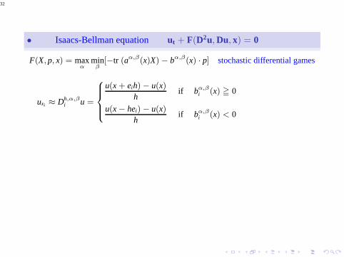
• Isaacs-Bellman equation ut + F(D2u, Du, x) = 0
F(X, p, x) = maxα
minβ
[−tr (aα,β(x)X) − bα,β(x) · p] stochastic differential games
uxi ≈ Dh,α,βi u =
8
>><
>>:
u(x + eih) − u(x)h
if bα,βi (x) ≧ 0
u(x − hei) − u(x)h
if bα,βi (x) < 0
33
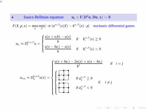
• Isaacs-Bellman equation ut + F(D2u, Du, x) = 0
F(X, p, x) = maxα
minβ
[−tr (aα,β(x)X) − bα,β(x) · p] stochastic differential games
uxi ≈ Dh,α,βi u =
8
>><
>>:
u(x + eih) − u(x)h
if bα,βi (x) ≧ 0
u(x − hei) − u(x)h
if bα,βi (x) < 0
uxixj ≈ Dh,αβij u(x) =
8
>>>>>>>>>><
>>>>>>>>>>:
u(x + hei) − 2u(x) + u(x − hei)
h2 if i = j
8
>>>>><
>>>>>:
if aα,βij ≧ 0
if aα,βij < 0
if i 6= j
34
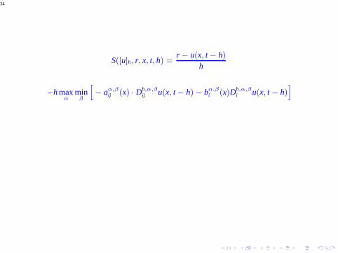
S([u]h, r, x, t, h) =r − u(x, t − h)
h
−h maxα
minβ
h
− aα,βij (x) · Dh,α,β
ij u(x, t − h) − bα,βi (x)Dh,α,β
i u(x, t − h)i
35
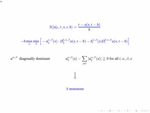
S([u]h, r, x, t, h) =r − u(x, t − h)
h
−h maxα
minβ
h
− aα,βij (x) · Dh,α,β
ij u(x, t − h) − bα,βi (x)Dh,α,β
i u(x, t − h)i
aα,β diagonally dominant aα,βii (x) −
X
j 6=i
|aα,βij (x)| ≧ 0 for all i, α, β, x
ww
S monotone

36
RATES OF CONVERGENCE – Hamilton-Jacobi
37
RATES OF CONVERGENCE – Hamilton-Jacobi
F(Du, u, x) = 0 S([uh]x, uh(x), x, h) = 0
38
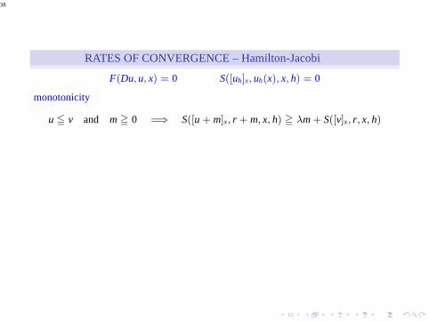
RATES OF CONVERGENCE – Hamilton-Jacobi
F(Du, u, x) = 0 S([uh]x, uh(x), x, h) = 0
monotonicity
u ≦ v and m ≧ 0 =⇒ S([u + m]x, r + m, x, h) ≧ λm + S([v]x, r, x, h)
39
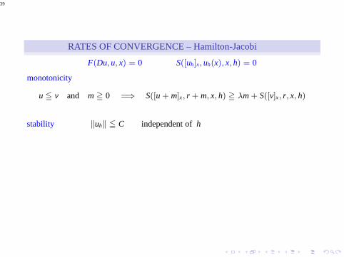
RATES OF CONVERGENCE – Hamilton-Jacobi
F(Du, u, x) = 0 S([uh]x, uh(x), x, h) = 0
monotonicity
u ≦ v and m ≧ 0 =⇒ S([u + m]x, r + m, x, h) ≧ λm + S([v]x, r, x, h)
stability ‖uh‖ ≦ C independent ofh
40
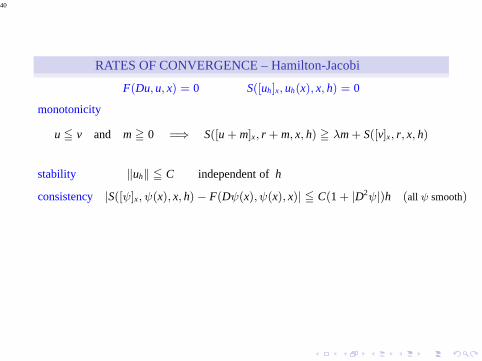
RATES OF CONVERGENCE – Hamilton-Jacobi
F(Du, u, x) = 0 S([uh]x, uh(x), x, h) = 0
monotonicity
u ≦ v and m ≧ 0 =⇒ S([u + m]x, r + m, x, h) ≧ λm + S([v]x, r, x, h)
stability ‖uh‖ ≦ C independent ofh
consistency |S([ψ]x, ψ(x), x, h) − F(Dψ(x), ψ(x), x)| ≦ C(1 + |D2ψ|)h (all ψ smooth)
41
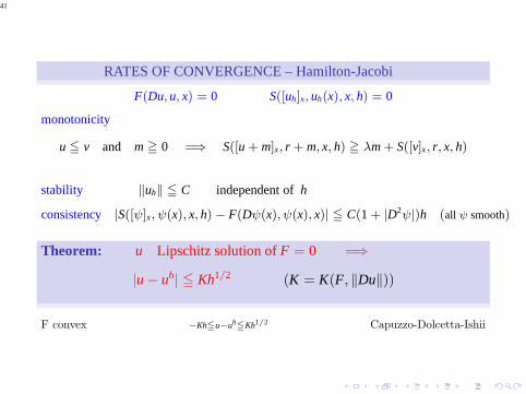
RATES OF CONVERGENCE – Hamilton-Jacobi
F(Du, u, x) = 0 S([uh]x, uh(x), x, h) = 0
monotonicity
u ≦ v and m ≧ 0 =⇒ S([u + m]x, r + m, x, h) ≧ λm + S([v]x, r, x, h)
stability ‖uh‖ ≦ C independent ofh
consistency |S([ψ]x, ψ(x), x, h) − F(Dψ(x), ψ(x), x)| ≦ C(1 + |D2ψ|)h (all ψ smooth)
Theorem: u Lipschitz solution ofF = 0 =⇒
|u − uh| ≦ Kh1/2 (K = K(F, ‖Du‖))
F convex −Kh≦u−uh≦Kh1/2 Capuzzo-Dolcetta-Ishii
42
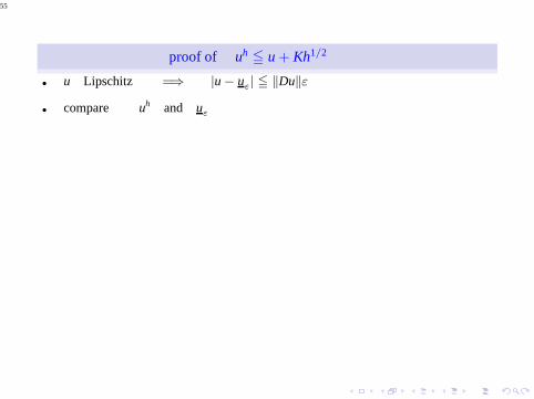
proof of uh ≦ u + Kh1/2
43
inf - and sup - convolution regularizations
44
inf - and sup - convolution regularizations
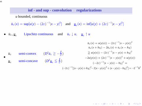
u bounded, continuous
uε(x) = sup[u(y) − (2ε)−1|x − y|2] and uε(x) = inf[u(y) + (2ε)−1|x − y|2]
45
inf - and sup - convolution regularizations
u bounded, continuous
uε(x) = sup[u(y) − (2ε)−1|x − y|2] and uε(x) = inf[u(y) + (2ε)−1|x − y|2]
• uε, uε Lipschitz continuous and uε ↓ u, uε ↑ u
46
inf - and sup - convolution regularizations
u bounded, continuous
uε(x) = sup[u(y) − (2ε)−1|x − y|2] and uε(x) = inf[u(y) + (2ε)−1|x − y|2]
• uε, uε Lipschitz continuous and uε ↓ u, uε ↑ u
•uε semi-convex (D2uε ≧ − I
ε )
uε semi-concave (D2uε ≦ Iε )
uε(x) = u(y(x)) − (2ε)−1
|x − y(x)|2
uε(x + hχ) − 2uε(x) + uε(x − hχ)
≧ u(y(x)) − (2ε)−1
|x − y(x) + hχ|2
−2u(y(x)) + (2ε)−1|x − y(x)|2 + u(y(x))
(−2ε)−1|x − y(x) − hχ|2 =
(−2ε)−1
[|x−y(x)+hχ|2−2|x−y(x)|2+|x−y(x)−hχ|
2]=−2−1h2
47
inf - and sup - convolution regularizations
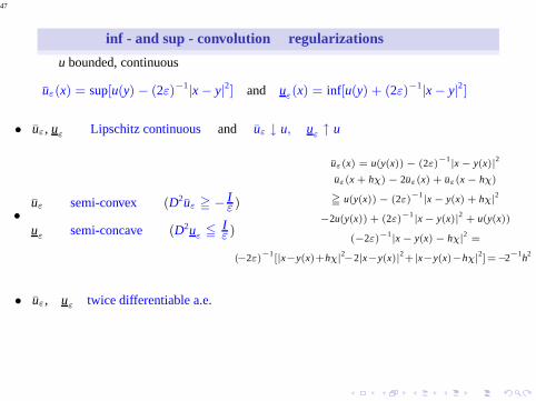
u bounded, continuous
uε(x) = sup[u(y) − (2ε)−1|x − y|2] and uε(x) = inf[u(y) + (2ε)−1|x − y|2]
• uε, uε Lipschitz continuous and uε ↓ u, uε ↑ u
•uε semi-convex (D2uε ≧ − I
ε )
uε semi-concave (D2uε ≦ Iε )
uε(x) = u(y(x)) − (2ε)−1
|x − y(x)|2
uε(x + hχ) − 2uε(x) + uε(x − hχ)
≧ u(y(x)) − (2ε)−1
|x − y(x) + hχ|2
−2u(y(x)) + (2ε)−1|x − y(x)|2 + u(y(x))
(−2ε)−1|x − y(x) − hχ|2 =
(−2ε)−1
[|x−y(x)+hχ|2−2|x−y(x)|2+|x−y(x)−hχ|
2]=−2−1h2
• uε, uε twice differentiable a.e.
48
inf - and sup - convolution regularizations
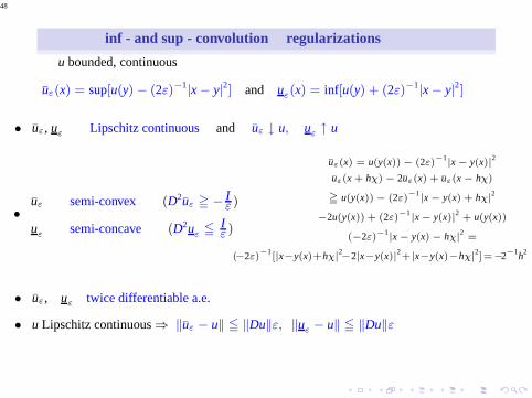
u bounded, continuous
uε(x) = sup[u(y) − (2ε)−1|x − y|2] and uε(x) = inf[u(y) + (2ε)−1|x − y|2]
• uε, uε Lipschitz continuous and uε ↓ u, uε ↑ u
•uε semi-convex (D2uε ≧ − I
ε )
uε semi-concave (D2uε ≦ Iε )
uε(x) = u(y(x)) − (2ε)−1
|x − y(x)|2
uε(x + hχ) − 2uε(x) + uε(x − hχ)
≧ u(y(x)) − (2ε)−1
|x − y(x) + hχ|2
−2u(y(x)) + (2ε)−1|x − y(x)|2 + u(y(x))
(−2ε)−1|x − y(x) − hχ|2 =
(−2ε)−1
[|x−y(x)+hχ|2−2|x−y(x)|2+|x−y(x)−hχ|
2]=−2−1h2
• uε, uε twice differentiable a.e.
• u Lipschitz continuous⇒ ‖uε − u‖ ≦ ‖Du‖ε, ‖uε − u‖ ≦ ‖Du‖ε
49
inf - and sup - convolution regularizations
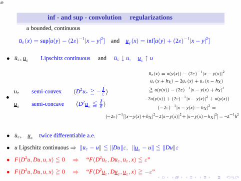
u bounded, continuous
uε(x) = sup[u(y) − (2ε)−1|x − y|2] and uε(x) = inf[u(y) + (2ε)−1|x − y|2]
• uε, uε Lipschitz continuous and uε ↓ u, uε ↑ u
•uε semi-convex (D2uε ≧ − I
ε )
uε semi-concave (D2uε ≦ Iε )
uε(x) = u(y(x)) − (2ε)−1
|x − y(x)|2
uε(x + hχ) − 2uε(x) + uε(x − hχ)
≧ u(y(x)) − (2ε)−1
|x − y(x) + hχ|2
−2u(y(x)) + (2ε)−1|x − y(x)|2 + u(y(x))
(−2ε)−1|x − y(x) − hχ|2 =
(−2ε)−1
[|x−y(x)+hχ|2−2|x−y(x)|2+|x−y(x)−hχ|
2]=−2−1h2
• uε, uε twice differentiable a.e.
• u Lipschitz continuous⇒ ‖uε − u‖ ≦ ‖Du‖ε, ‖uε − u‖ ≦ ‖Du‖ε
• F(D2u,Du, u, x) ≦ 0 ⇒ “F(D2uε,Duε, uε, x) ≦ ε”
• F(D2u,Du, u, x) ≧ 0 ⇒ “F(D2uε,Duε, uε, x) ≧ −ε”
50
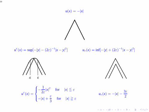
u(x) = −|x|
uε(x) = sup[−|y| − (2ε)−1|x − y|2] uε(x) = inf[−|y| + (2ε)−1|x − y|2]
uε(x) =
8
><
>:
−12ε
|x|2 for |x| ≦ ε
−|x| +ε
3for |x| ≧ ε
uε(x) = −|x| −3ε2
51
parallel surface regularization
52
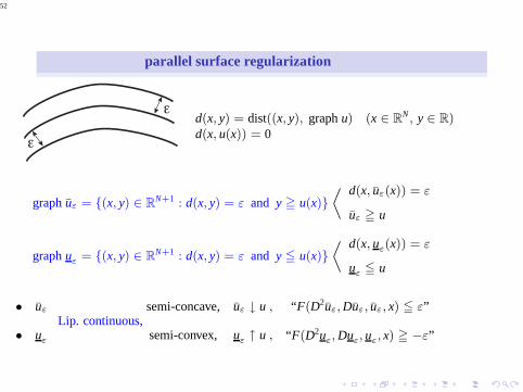
parallel surface regularization
d(x, y) = dist((x, y), graphu) (x ∈ RN , y ∈ R)
d(x, u(x)) = 0
graphuε = (x, y) ∈ RN+1 : d(x, y) = ε and y ≧ u(x)
fi d(x, uε(x)) = ε
uε ≧ u
graphuε = (x, y) ∈ RN+1 : d(x, y) = ε and y ≦ u(x)
fi d(x, uε(x)) = ε
uε ≦ u
• uε
• uε
Lip. continuous,semi-concave,
semi-convex,
uε ↓ u ,
uε ↑ u ,
“F(D2uε,Duε, uε, x) ≦ ε”
“F(D2uε,Duε, uε, x) ≧ −ε”

53
proof of uh ≦ u + Kh1/2
54
proof of uh ≦ u + Kh1/2
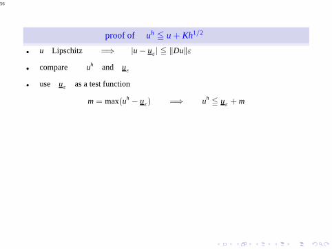
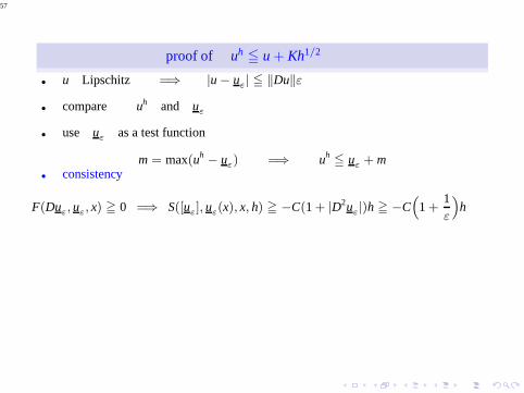
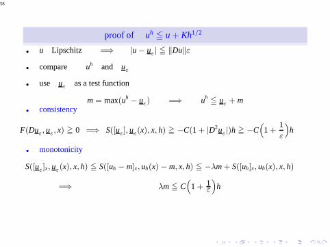
• u Lipschitz =⇒ |u − uε| ≦ ‖Du‖ε
55
proof of uh ≦ u + Kh1/2
• u Lipschitz =⇒ |u − uε| ≦ ‖Du‖ε
• compare uh and uε
56
proof of uh ≦ u + Kh1/2
• u Lipschitz =⇒ |u − uε| ≦ ‖Du‖ε
• compare uh and uε
• use uε as a test function
m = max(uh − uε) =⇒ uh≦ uε + m
57
proof of uh ≦ u + Kh1/2
• u Lipschitz =⇒ |u − uε| ≦ ‖Du‖ε
• compare uh and uε
• use uε as a test function
m = max(uh − uε) =⇒ uh≦ uε + m
• consistency
F(Duε, uε, x) ≧ 0 =⇒ S([uε], uε(x), x, h) ≧ −C(1+ |D2uε|)h ≧ −C“
1 +1ε
”
h
58
proof of uh ≦ u + Kh1/2
• u Lipschitz =⇒ |u − uε| ≦ ‖Du‖ε
• compare uh and uε
• use uε as a test function
m = max(uh − uε) =⇒ uh≦ uε + m
• consistency
F(Duε, uε, x) ≧ 0 =⇒ S([uε], uε(x), x, h) ≧ −C(1+ |D2uε|)h ≧ −C“
1 +1ε
”
h
• monotonicity
S([uε]x, uε(x), x, h) ≦ S([uh − m]x, uh(x) − m, x, h) ≦ −λm + S([uh]x, uh(x), x, h)
=⇒ λm ≦ C“
1 + 1ε
”
h
59
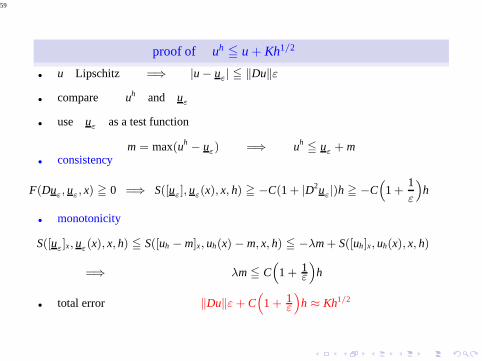
proof of uh ≦ u + Kh1/2
• u Lipschitz =⇒ |u − uε| ≦ ‖Du‖ε
• compare uh and uε
• use uε as a test function
m = max(uh − uε) =⇒ uh≦ uε + m
• consistency
F(Duε, uε, x) ≧ 0 =⇒ S([uε], uε(x), x, h) ≧ −C(1+ |D2uε|)h ≧ −C“
1 +1ε
”
h
• monotonicity
S([uε]x, uε(x), x, h) ≦ S([uh − m]x, uh(x) − m, x, h) ≦ −λm + S([uh]x, uh(x), x, h)
=⇒ λm ≦ C“
1 + 1ε
”
h
• total error ‖Du‖ε + C“
1 + 1ε
”
h ≈ Kh1/2
60
RATES OF CONVERGENCE – uniformly elliptic equations
61
RATES OF CONVERGENCE – uniformly elliptic equations
F(D2u,Du, x) = 0 S([uh]x, uh(x), x, h) = 0
consistency
|S([φ]x, φ(x), x, h) − F(D2φ(x),Dφ(x), x)| ≦ K(1 + |D3φ|)h
62
RATES OF CONVERGENCE – uniformly elliptic equations
F(D2u,Du, x) = 0 S([uh]x, uh(x), x, h) = 0
consistency
|S([φ]x, φ(x), x, h) − F(D2φ(x),Dφ(x), x)| ≦ K(1 + |D3φ|)h
problem no regularization of viscosity solutionscontrolling “third-derivatives” and “preserving” equation
63
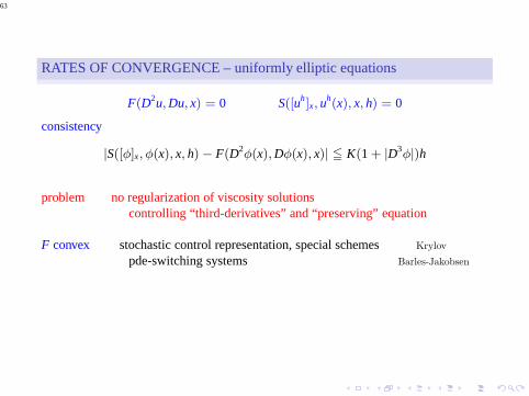
RATES OF CONVERGENCE – uniformly elliptic equations
F(D2u,Du, x) = 0 S([uh]x, uh(x), x, h) = 0
consistency
|S([φ]x, φ(x), x, h) − F(D2φ(x),Dφ(x), x)| ≦ K(1 + |D3φ|)h
problem no regularization of viscosity solutionscontrolling “third-derivatives” and “preserving” equation
F convex stochastic control representation, special schemes Krylov
pde-switching systems Barles-Jakobsen
64
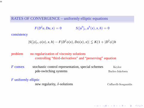
RATES OF CONVERGENCE – uniformly elliptic equations
F(D2u,Du, x) = 0 S([uh]x, uh(x), x, h) = 0
consistency
|S([φ]x, φ(x), x, h) − F(D2φ(x),Dφ(x), x)| ≦ K(1 + |D3φ|)h
problem no regularization of viscosity solutionscontrolling “third-derivatives” and “preserving” equation
F convex stochastic control representation, special schemes Krylov
pde-switching systems Barles-Jakobsen
F uniformly ellipticnew regularity,δ-solutions Caffarelli-Souganidis
65
GENERAL STRATEGY
(∗)
8
<
:
F(D2u) = f in U
u = g on ∂UF uniformly elliptic
66
GENERAL STRATEGY
(∗)
8
<
:
F(D2u) = f in U
u = g on ∂UF uniformly elliptic
• δ-viscosity solutions
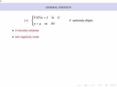
67
GENERAL STRATEGY
(∗)
8
<
:
F(D2u) = f in U
u = g on ∂UF uniformly elliptic
• δ-viscosity solutions
• new regularity result
68
GENERAL STRATEGY
(∗)
8
<
:
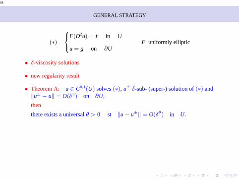
F(D2u) = f in U
u = g on ∂UF uniformly elliptic
• δ-viscosity solutions
• new regularity result
• Theorem A: u ∈ C0,1(U) solves(∗), u± δ-sub- (super-) solution of(∗) and‖u± − u‖ = O(δη) on ∂U,
then
there exists a universalθ > 0 st ‖u − u±‖ = O(δθ) in U.
69
GENERAL STRATEGY
(∗)
8
<
:
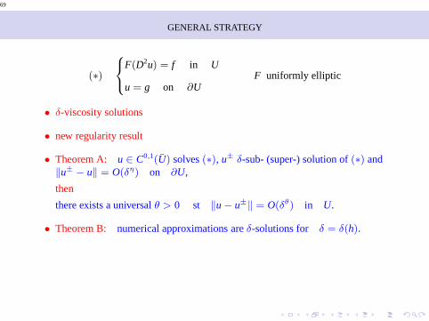
F(D2u) = f in U
u = g on ∂UF uniformly elliptic
• δ-viscosity solutions
• new regularity result
• Theorem A: u ∈ C0,1(U) solves(∗), u± δ-sub- (super-) solution of(∗) and‖u± − u‖ = O(δη) on ∂U,
then
there exists a universalθ > 0 st ‖u − u±‖ = O(δθ) in U.
• Theorem B: numerical approximations areδ-solutions for δ = δ(h).
70
GENERAL STRATEGY
(∗)
8
<
:
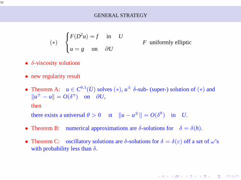
F(D2u) = f in U
u = g on ∂UF uniformly elliptic
• δ-viscosity solutions
• new regularity result
• Theorem A: u ∈ C0,1(U) solves(∗), u± δ-sub- (super-) solution of(∗) and‖u± − u‖ = O(δη) on ∂U,
then
there exists a universalθ > 0 st ‖u − u±‖ = O(δθ) in U.
• Theorem B: numerical approximations areδ-solutions for δ = δ(h).
• Theorem C: oscillatory solutions areδ-solutions forδ = δ(ε) off a set ofω’swith probability less thanδ.
71
δ-viscosity solution ofF(D2u) = f in U
72
δ-viscosity solution ofF(D2u) = f in U
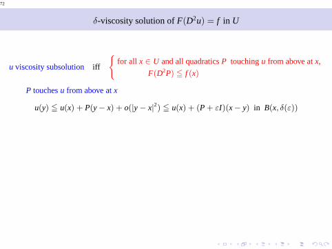
u viscosity subsolution iff
(
for all x ∈ U and all quadraticsP touchingu from above atx,
F(D2P) ≦ f (x)
P touchesu from above atx
u(y) ≦ u(x) + P(y − x) + o(|y − x|2) ≦ u(x) + (P + εI)(x − y) in B(x, δ(ε))
73
δ-viscosity solution ofF(D2u) = f in U
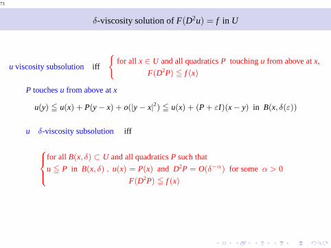
u viscosity subsolution iff
(
for all x ∈ U and all quadraticsP touchingu from above atx,
F(D2P) ≦ f (x)
P touchesu from above atx
u(y) ≦ u(x) + P(y − x) + o(|y − x|2) ≦ u(x) + (P + εI)(x − y) in B(x, δ(ε))
u δ-viscosity subsolution iff
8
><
>:
for all B(x, δ) ⊂ U and all quadraticsP such that
u ≦ P in B(x, δ) , u(x) = P(x) and D2P = O(δ−α) for someα > 0
F(D2P) ≦ f (x)
74
δ-viscosity solution ofF(D2u) = f in U
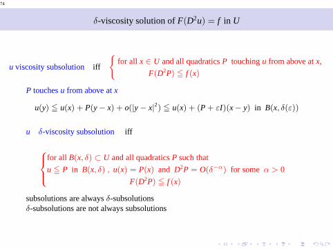
u viscosity subsolution iff
(
for all x ∈ U and all quadraticsP touchingu from above atx,
F(D2P) ≦ f (x)
P touchesu from above atx
u(y) ≦ u(x) + P(y − x) + o(|y − x|2) ≦ u(x) + (P + εI)(x − y) in B(x, δ(ε))
u δ-viscosity subsolution iff
8
><
>:
for all B(x, δ) ⊂ U and all quadraticsP such that
u ≦ P in B(x, δ) , u(x) = P(x) and D2P = O(δ−α) for someα > 0
F(D2P) ≦ f (x)
subsolutions are alwaysδ-subsolutionsδ-subsolutions are not always subsolutions
75
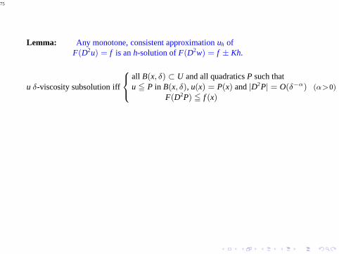
Lemma: Any monotone, consistent approximationuh ofF(D2u) = f is anh-solution ofF(D2w) = f ± Kh.
u δ-viscosity subsolution iff
8
<
:
all B(x, δ) ⊂ U and all quadraticsP such thatu ≦ P in B(x, δ), u(x) = P(x) and|D2P| = O(δ−α) (α>0)
F(D2P) ≦ f (x)
76
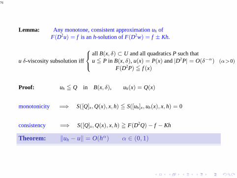
Lemma: Any monotone, consistent approximationuh ofF(D2u) = f is anh-solution ofF(D2w) = f ± Kh.
u δ-viscosity subsolution iff
8
<
:
all B(x, δ) ⊂ U and all quadraticsP such thatu ≦ P in B(x, δ), u(x) = P(x) and|D2P| = O(δ−α) (α>0)
F(D2P) ≦ f (x)
Proof: uh ≦ Q in B(x, δ), uh(x) = Q(x)
monotonicity =⇒ S([Q]x,Q(x), x, h) ≦ S([uh]x, uh(x), x, h) = 0
consistency =⇒ S([Q]x,Q(x), x, h) ≧ F(D2Q) − f − Kh
Theorem: ‖uh − u‖ = O(hα) α ∈ (0, 1)
77
HOMOGENIZATION
F(D2uε,xε, ω) = 0 in U F uniformly elliptic, stationary ergodic
uε −→ε→0
u0 a.s. and F0(D2u0) = 0 in U
78
HOMOGENIZATION
F(D2uε,xε, ω) = 0 in U F uniformly elliptic, stationary ergodic
uε −→ε→0
u0 a.s. and F0(D2u0) = 0 in U
• For eachQ ∈ SN , F0(Q) is the unique constant st
if
8
<
:
F(D2uε,xε , ω) = F0(Q) in B1
uε = Q on ∂B1
, then ‖uε(·, ω) − Q‖C(B1)→ 0 a.s.
if
8
<
:
F(D2uε, x, ω) = F0(Q) in B1/ε ,
uε = Q on ∂B1/ε
then ‖ε2uε(·, ω) − Q‖C(B1/ε) → 0 a.s.
uε(x) = ε2uε( xε )
!
Caffarelli-Souganidis-Wang
79
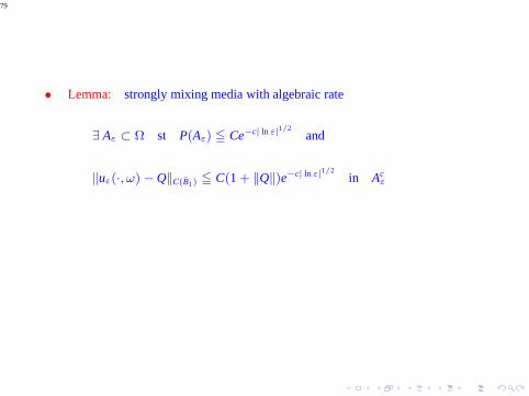
• Lemma: strongly mixing media with algebraic rate
∃ Aε ⊂ Ω st P(Aε) ≦ Ce−c| ln ε|1/2and
‖uε(·, ω) − Q‖C(B1)≦ C(1 + ‖Q‖)e−c| ln ε|1/2
in Acε
80
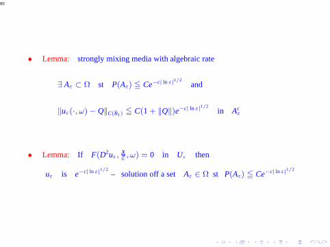
• Lemma: strongly mixing media with algebraic rate
∃ Aε ⊂ Ω st P(Aε) ≦ Ce−c| ln ε|1/2and
‖uε(·, ω) − Q‖C(B1)≦ C(1 + ‖Q‖)e−c| ln ε|1/2
in Acε
• Lemma: If F(D2uε,xε , ω) = 0 in U, then
uε is e−c| ln ε|1/2– solution off a set Aε ∈ Ω st P(Aε) ≦ Ce−c| ln ε|1/2
81
back to sup- and inf-convolutionssome key properties of the regularizations
of Lipschitz sub- and super-solutions
82
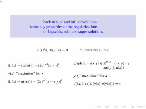
back to sup- and inf-convolutionssome key properties of the regularizations
of Lipschitz sub- and super-solutions
F(D2u,Du, u, x) = 0 F uniformly elliptic
uε(x) = sup[u(y) − (2ε)−1|x − y|2]
y(x) “maximizer” for x
uε(x) = u(y(x)) − (2ε)−1|x − y(x)|2
graphuε =(x, y) ∈ RN+1 : d(x, y)=ε
andy ≧ u(x)
y(x) “maximizer” for x
d((x, uε(x)), (y(x), u(y(x))) = ε
83
∃ C > 0 (depending ONLY on ellipticity constants andN) st
• |x1 − x2| ≦ C|y(x1) − y(x2)| (Jacobian of y 7→ y−1(x) is bdd)
• if a quadraticP touchesuε from above atx, thenu is touchedaty(x) from above by a quadraticPε
and
D2uε(x) ≧ D2u(y(x)) + Cε2|D2u(y(x))|2
• ∃ t0, σ st for t ≧ t0 ∃ Aεt st |Aε
t | ≦ t−σ and
uε has a second order expansion from above with error of sizet in Aε,ct
uε has a second order expansion from below with error of sizet in Aε,ct
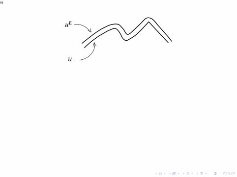
84
u
>
>
85
u
>
>
x
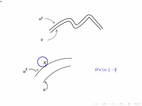
u
>
> D2uε(x) ≧ − cε
86
u
>
>
x
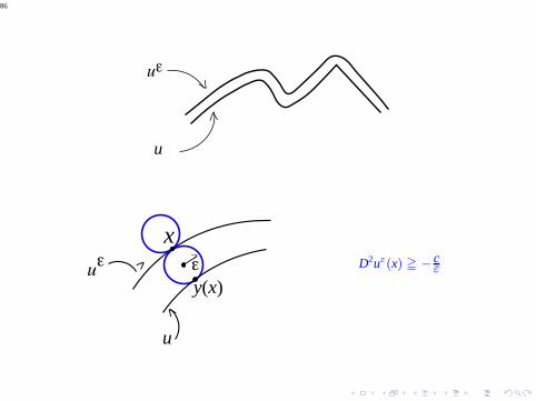
u
y(x)
>
>
> D2uε(x) ≧ − cε
87
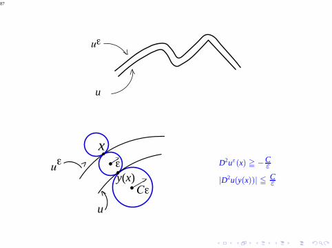
u
>
>
x
u
y(x) >
>
>
> D2uε(x) ≧ −Cε
|D2u(y(x))| ≦ Cε
88
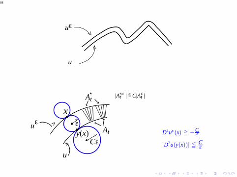
u
>
>
x
u
y(x) >
>
>
>At
At* |At | < C|At |*,c c
=
D2uε(x) ≧ −Cε
|D2u(y(x))| ≦ Cε

89
Sketch of proof
90
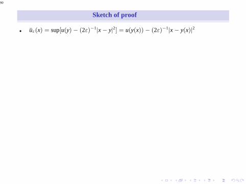
Sketch of proof
• uε(x) = sup[u(y) − (2ε)−1|x − y|2] = u(y(x)) − (2ε)−1|x − y(x)|2
91
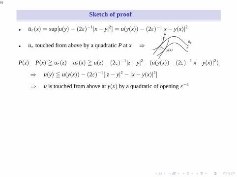
Sketch of proof
• uε(x) = sup[u(y) − (2ε)−1|x − y|2] = u(y(x)) − (2ε)−1|x − y(x)|2
• uε touched from above by a quadraticP at x ⇒
P
x y(x)u
uε−
P(z)−P(x) ≧ uε(z)− uε(x) ≧ u(z)− (2ε)−1|z− y|2− (u(y(x))− (2ε)−1|x− y(x)|2)
⇒ u(y) ≦ u(y(x)) − (2ε)−1[|z − y|2 − |x − y(x)|2]
⇒ u is touched from above aty(x) by a quadratic of openingε−1
92
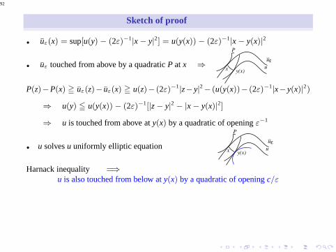
Sketch of proof
• uε(x) = sup[u(y) − (2ε)−1|x − y|2] = u(y(x)) − (2ε)−1|x − y(x)|2
• uε touched from above by a quadraticP at x ⇒
P
x y(x)u
uε−
P(z)−P(x) ≧ uε(z)− uε(x) ≧ u(z)− (2ε)−1|z− y|2− (u(y(x))− (2ε)−1|x− y(x)|2)
⇒ u(y) ≦ u(y(x)) − (2ε)−1[|z − y|2 − |x − y(x)|2]
⇒ u is touched from above aty(x) by a quadratic of openingε−1
• u solvesu uniformly elliptic equation
P
x y(x)u
uε−
Harnack inequality =⇒u is also touched from below aty(x) by a quadratic of openingc/ε
93
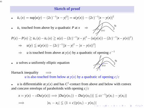
Sketch of proof
• uε(x) = sup[u(y) − (2ε)−1|x − y|2] = u(y(x)) − (2ε)−1|x − y(x)|2
• uε touched from above by a quadraticP at x ⇒
P
x y(x)u
uε−
P(z)−P(x) ≧ uε(z)− uε(x) ≧ u(z)− (2ε)−1|z− y|2− (u(y(x))− (2ε)−1|x− y(x)|2)
⇒ u(y) ≦ u(y(x)) − (2ε)−1[|z − y|2 − |x − y(x)|2]
⇒ u is touched from above aty(x) by a quadratic of openingε−1
• u solvesu uniformly elliptic equation
P
x y(x)u
uε−
Harnack inequality =⇒u is also touched from below aty(x) by a quadratic of openingc/ε
• u is differentiable aty(x) and hasC1-contact from above and below with convexand concave envelops of paraboloids with openingc/ε
x = y(x) − εDu(y(x)) =⇒ |Du(y(x1)) − Du(y(x2))| ≦ cε−1|y(x1) − y(x2)|
=⇒ |x1 − x2| ≦ (1 + c)|y(x1) − y(x2)|
94
(NEW) REGULARITY RESULT
F(D2u) = f in U
95
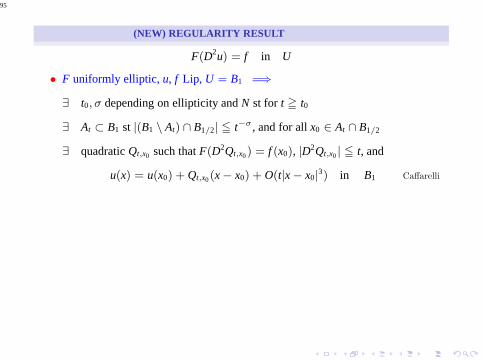
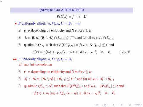
(NEW) REGULARITY RESULT
F(D2u) = f in U
• F uniformly elliptic, u, f Lip, U = B1 =⇒
∃ t0, σ depending on ellipticity andN st for t ≧ t0
∃ At ⊂ B1 st |(B1 \ At) ∩ B1/2| ≦ t−σ , and for allx0 ∈ At ∩ B1/2
∃ quadraticQt,x0 such thatF(D2Qt,x0) = f (x0), |D2Qt,x0| ≦ t, and
u(x) = u(x0) + Qt,x0(x − x0) + O(t|x − x0|3) in B1 Caffarelli
96
(NEW) REGULARITY RESULT
F(D2u) = f in U
• F uniformly elliptic, u, f Lip, U = B1 =⇒
∃ t0, σ depending on ellipticity andN st for t ≧ t0
∃ At ⊂ B1 st |(B1 \ At) ∩ B1/2| ≦ t−σ , and for allx0 ∈ At ∩ B1/2
∃ quadraticQt,x0 such thatF(D2Qt,x0) = f (x0), |D2Qt,x0| ≦ t, and
u(x) = u(x0) + Qt,x0(x − x0) + O(t|x − x0|3) in B1 Caffarelli
•• F uniformly elliptic, u, f Lip, U = B1
u±ε sup, inf-convolution
∃ t0, σ depending on ellipticity andN st for t ≧ t0
∃ Aεt ⊂ B1 st |(B1 \ Aε
t ) ∩ B1/2| ≦ t−σ and for allx0 ∈ Aεt ∩ B1/2
∃ quadraticQεt,x0
∈ SN such thatF(D2Qεt,x0
) ≈ f (x0), |D2Qεt,x0
| ≦ t and
u±ε (x) ≈ uε(x0) + Qε
t,x0(x − x0) + O(t|x − x0|
3) in B1
97
Proof of regularity result
F(D2u) = f in B1
98
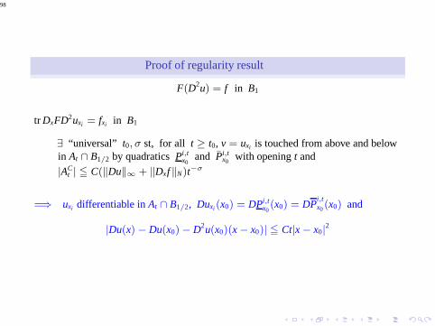
Proof of regularity result
F(D2u) = f in B1
tr DxFD2uxi = fxi in B1
∃ “universal” t0, σ st, for all t ≥ t0, v = uxi is touched from above and belowin At ∩ B1/2 by quadraticsPi,t
x0and Pi,t
x0with openingt and
|ACt | ≦ C(‖Du‖∞ + ‖Dxf‖N)t−σ
=⇒ uxi differentiable inAt ∩ B1/2, Duxi(x0) = DPi,tx0
(x0) = DPi,tx0
(x0) and
|Du(x) − Du(x0) − D2u(x0)(x − x0)| ≦ Ct|x − x0|2
99
Sketch of proof of
u solution,v δ-supersolution ofF(D2w) = f in Uu ≦ v + O(δγ) on∂U
ff
=⇒ u ≦ v + cδθ (θ > 0)
• several approximations/regularizations
u −→ u subsolution F(D2w) = f − δβ D2u ≧ −δ−2ζI
v −→ v δ-supersolution F(D2v) = f D2v ≦ δ2ζI
100
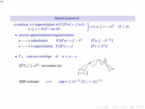
Sketch of proof of
u solution,v δ-supersolution ofF(D2w) = f in Uu ≦ v + O(δγ) on∂U
ff
=⇒ u ≦ v + cδθ (θ > 0)
• several approximations/regularizations
u −→ u subsolution F(D2w) = f − δβ D2u ≧ −δ−2ζI
v −→ v δ-supersolution F(D2v) = f D2v ≦ δ2ζI
• Γw concave envelope ofw = u − v
|D2Γw| ≦ cδ2ζ on contact set
ABP-estimate =⇒ supw ≦ cδ−2ζ |Γw = w|1/N
101
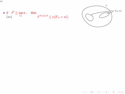
• if δθ ≦ supUδ
w , then(∗∗) δ(θ+2ζ)N
≦ c|Γw = w|
Γw =w
U
102
• if δθ ≦ supUδ
w , then(∗∗) δ(θ+2ζ)N
≦ c|Γw = w|
• covering argument and(∗∗) =⇒
∃ B(xi, δγ) st |B(xi,
12δ
γ) ∩ Γw = w| ≧ cδ(θ+2ζ+γ)N
Γw =w
B(xi, 2-1δγ)
U
103
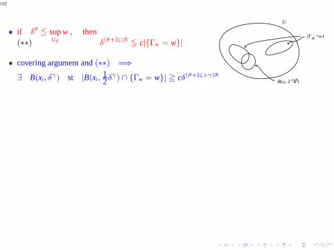
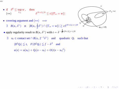
• if δθ ≦ supUδ
w , then(∗∗) δ(θ+2ζ)N
≦ c|Γw = w|
• covering argument and(∗∗) =⇒
∃ B(xi, δγ) st |B(xi,
12δ
γ) ∩ Γw = w| ≧ cδ(θ+2ζ+γ)N
Γw =w
B(xi, 2-1δγ)At
x0
U
• apply regularity result toB(xi, δγ) with t = δ−
1σ (θ+2ζ+γ)N
∃ x0 ∈ contact set∩ B(xi, 2−1δγ) and quadraticQt such that
|D2Qt| ≦ t, F(D2Qt) ≦ f − δβ and
u(x) = u(x0) + Qt(x − x0) + O(t|x − x0|3)
104
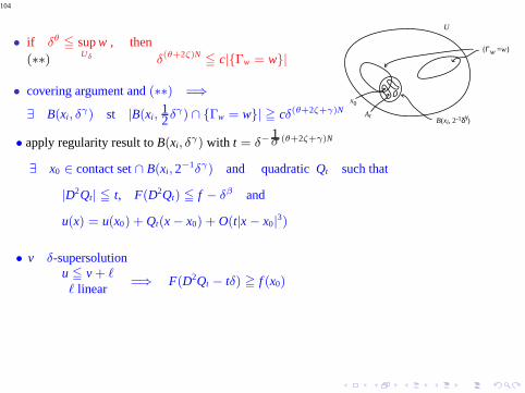
• if δθ ≦ supUδ
w , then(∗∗) δ(θ+2ζ)N
≦ c|Γw = w|
• covering argument and(∗∗) =⇒
∃ B(xi, δγ) st |B(xi,
12δ
γ) ∩ Γw = w| ≧ cδ(θ+2ζ+γ)N
Γw =w
B(xi, 2-1δγ)At
x0
U
• apply regularity result toB(xi, δγ) with t = δ−
1σ (θ+2ζ+γ)N
∃ x0 ∈ contact set∩ B(xi, 2−1δγ) and quadraticQt such that
|D2Qt| ≦ t, F(D2Qt) ≦ f − δβ and
u(x) = u(x0) + Qt(x − x0) + O(t|x − x0|3)
• v δ-supersolutionu ≦ v + ℓℓ linear
=⇒ F(D2Qt − tδ) ≧ f (x0)
105
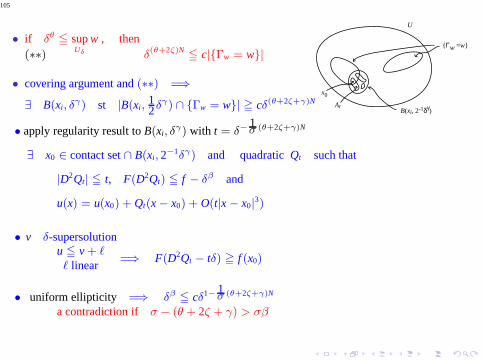
• if δθ ≦ supUδ
w , then(∗∗) δ(θ+2ζ)N
≦ c|Γw = w|
• covering argument and(∗∗) =⇒
∃ B(xi, δγ) st |B(xi,
12δ
γ) ∩ Γw = w| ≧ cδ(θ+2ζ+γ)N
Γw =w
B(xi, 2-1δγ)At
x0
U
• apply regularity result toB(xi, δγ) with t = δ−
1σ (θ+2ζ+γ)N
∃ x0 ∈ contact set∩ B(xi, 2−1δγ) and quadraticQt such that
|D2Qt| ≦ t, F(D2Qt) ≦ f − δβ and
u(x) = u(x0) + Qt(x − x0) + O(t|x − x0|3)
• v δ-supersolutionu ≦ v + ℓℓ linear
=⇒ F(D2Qt − tδ) ≧ f (x0)
• uniform ellipticity =⇒ δβ ≦ cδ1− 1σ (θ+2ζ+γ)N
a contradiction if σ − (θ + 2ζ + γ) > σβ
106
HOMOGENIZATION
8
<
:
F(D2uε,xε , ω) = 0 in U
uε = g on ∂UF uniformly elliptic, stationary, ergodic
107
HOMOGENIZATION
8
<
:
F(D2uε,xε , ω) = 0 in U
uε = g on ∂UF uniformly elliptic, stationary, ergodic
∃ F0 uniformly elliptic st
uε → u0ε→0
in C(U) and a.s.
8
<
:
F0(D2u0) = 0 in U
u0 = g on ∂UCaffarelli-Souganidis-Wang
108
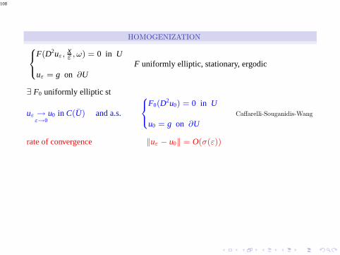
HOMOGENIZATION
8
<
:
F(D2uε,xε , ω) = 0 in U
uε = g on ∂UF uniformly elliptic, stationary, ergodic
∃ F0 uniformly elliptic st
uε → u0ε→0
in C(U) and a.s.
8
<
:
F0(D2u0) = 0 in U
u0 = g on ∂UCaffarelli-Souganidis-Wang
rate of convergence ‖uε − u0‖ = O(σ(ε))
109
HOMOGENIZATION
8
<
:
F(D2uε,xε , ω) = 0 in U
uε = g on ∂UF uniformly elliptic, stationary, ergodic
∃ F0 uniformly elliptic st
uε → u0ε→0
in C(U) and a.s.
8
<
:
F0(D2u0) = 0 in U
u0 = g on ∂UCaffarelli-Souganidis-Wang
rate of convergence ‖uε − u0‖ = O(σ(ε))
strongly mixing with algebraic rate*
F linear σ(ε) = εγYurinskii
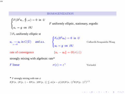
* F strongly mixing with rateφ
E[F(x, ·)F(y, ·) − EF(x, ·)EF(y, ·)] ≦ φ(|x − y|)(E(F(x, ·))2E(F(y, ·))2)1/2
110
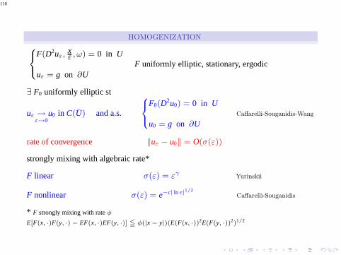
HOMOGENIZATION
8
<
:
F(D2uε,xε , ω) = 0 in U
uε = g on ∂UF uniformly elliptic, stationary, ergodic
∃ F0 uniformly elliptic st
uε → u0ε→0
in C(U) and a.s.
8
<
:
F0(D2u0) = 0 in U
u0 = g on ∂UCaffarelli-Souganidis-Wang
rate of convergence ‖uε − u0‖ = O(σ(ε))
strongly mixing with algebraic rate*
F linear σ(ε) = εγYurinskii
F nonlinear σ(ε) = e−c| ln ε|1/2Caffarelli-Souganidis
* F strongly mixing with rateφ
E[F(x, ·)F(y, ·) − EF(x, ·)EF(y, ·)] ≦ φ(|x − y|)(E(F(x, ·))2E(F(y, ·))2)1/2
111
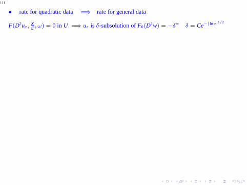
• rate for quadratic data =⇒ rate for general data
F(D2uε,xε , ω) = 0 in U =⇒ uε is δ-subsolution ofF0(D2w) = −δα δ = Ce−| ln ε|1/2
112
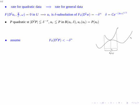
• rate for quadratic data =⇒ rate for general data
F(D2uε,xε , ω) = 0 in U =⇒ uε is δ-subsolution ofF0(D2w) = −δα δ = Ce−| ln ε|1/2
• P quadratic st|D2P| ≦ δ−σ , uε ≦ P in B(x0, δ), uε(x0) = P(x0)
• assume F0(D2P) < −δα
P
Bδ(x0)
x0
uε
113
• rate for quadratic data =⇒ rate for general data
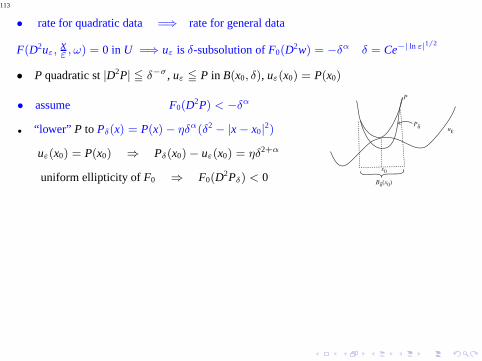
F(D2uε,xε , ω) = 0 in U =⇒ uε is δ-subsolution ofF0(D2w) = −δα δ = Ce−| ln ε|1/2
• P quadratic st|D2P| ≦ δ−σ , uε ≦ P in B(x0, δ), uε(x0) = P(x0)
• assume F0(D2P) < −δα
• “lower” P to Pδ(x) = P(x) − ηδα(δ2 − |x − x0|2)
uε(x0) = P(x0) ⇒ Pδ(x0) − uε(x0) = ηδ2+α
uniform ellipticity of F0 ⇒ F0(D2Pδ) < 0
P
Pδ
Bδ(x0)
x0
uε
114
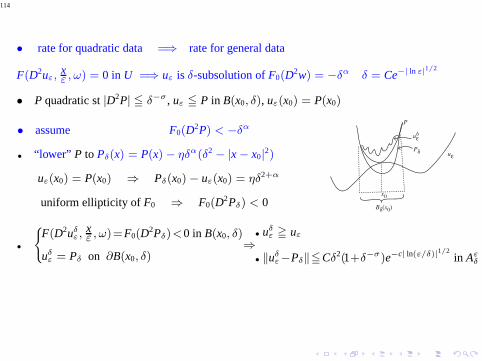
• rate for quadratic data =⇒ rate for general data
F(D2uε,xε , ω) = 0 in U =⇒ uε is δ-subsolution ofF0(D2w) = −δα δ = Ce−| ln ε|1/2
• P quadratic st|D2P| ≦ δ−σ , uε ≦ P in B(x0, δ), uε(x0) = P(x0)
• assume F0(D2P) < −δα
• “lower” P to Pδ(x) = P(x) − ηδα(δ2 − |x − x0|2)
uε(x0) = P(x0) ⇒ Pδ(x0) − uε(x0) = ηδ2+α
uniform ellipticity of F0 ⇒ F0(D2Pδ) < 0
P
Pδ
Bδ(x0)
x0
uε
uεδ
•
(F(D2uδ
ε,xε , ω)=F0(D2Pδ)<0 in B(x0, δ)
uδε = Pδ on ∂B(x0, δ)
⇒• uδ
ε ≧ uε
• ‖uδε−Pδ‖≦Cδ2(1+δ−σ)e−c| ln(ε/δ)|1/2
in Aεδ
115
• rate for quadratic data =⇒ rate for general data
F(D2uε,xε , ω) = 0 in U =⇒ uε is δ-subsolution ofF0(D2w) = −δα δ = Ce−| ln ε|1/2
• P quadratic st|D2P| ≦ δ−σ , uε ≦ P in B(x0, δ), uε(x0) = P(x0)
• assume F0(D2P) < −δα
• “lower” P to Pδ(x) = P(x) − ηδα(δ2 − |x − x0|2)
uε(x0) = P(x0) ⇒ Pδ(x0) − uε(x0) = ηδ2+α
uniform ellipticity of F0 ⇒ F0(D2Pδ) < 0
P
Pδ
Bδ(x0)
x0
uε
uεδ
•
(F(D2uδ
ε,xε , ω)=F0(D2Pδ)<0 in B(x0, δ)
uδε = Pδ on ∂B(x0, δ)
⇒• uδ
ε ≧ uε
• ‖uδε−Pδ‖≦Cδ2(1+δ−σ)e−c| ln(ε/δ)|1/2
in Aεδ
• 0 ≦ uδε(x0) − uε(x0) = uδ
ε(x0) − P(x0) + P(x0) − uε(x0)
≦ Cδ2(1 + δ−σ)e−c| ln(ε/δ)|1/2− ηδα+2< 0 for δ = Ce−c| ln ε|1/2
116
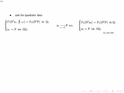
• rate for quadratic data8
<
:
F(D2uε,xε , ω) = F0(D2P) in Q1
uε = P on ∂Q1
uε −→ε→0
P a.s.
8
<
:
F0(D2u0) = F0(D2P) in Q1
u0 = P on ∂Q1
Q1 unit cube
117
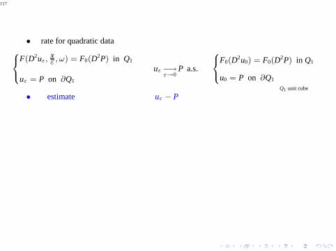
• rate for quadratic data8
<
:
F(D2uε,xε , ω) = F0(D2P) in Q1
uε = P on ∂Q1
uε −→ε→0
P a.s.
8
<
:
F0(D2u0) = F0(D2P) in Q1
u0 = P on ∂Q1
Q1 unit cube
• estimate uε − P
118
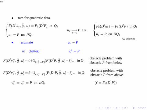
• rate for quadratic data8
<
:
F(D2uε,xε , ω) = F0(D2P) in Q1
uε = P on ∂Q1
uε −→ε→0
P a.s.
8
<
:
F0(D2u0) = F0(D2P) in Q1
u0 = P on ∂Q1
Q1 unit cube
• estimate uε − P
or (better) v±ε − P
F(D2v+ε ,
xε , ω)=ℓ+1
v+ε =P(F(D2P, xε , ω)−ℓ)+ in Q1
obstacle problem withobstacleP from below
F(D2v−ε ,xε , ω)=ℓ−1
v−ε =P(F(D2P, xε , ω)−ℓ)− in Q1
obstacle problem withobstacleP from above
v+ε = v−ε = P on ∂Q1 (ℓ = F0(D2P))
119
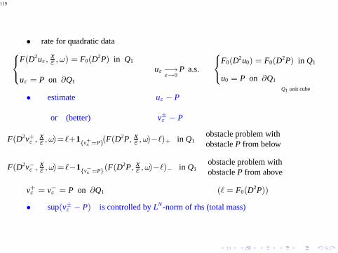
• rate for quadratic data8
<
:
F(D2uε,xε , ω) = F0(D2P) in Q1
uε = P on ∂Q1
uε −→ε→0
P a.s.
8
<
:
F0(D2u0) = F0(D2P) in Q1
u0 = P on ∂Q1
Q1 unit cube
• estimate uε − P
or (better) v±ε − P
F(D2v+ε ,
xε , ω)=ℓ+1
v+ε =P(F(D2P, xε , ω)−ℓ)+ in Q1
obstacle problem withobstacleP from below
F(D2v−ε ,xε , ω)=ℓ−1
v−ε =P(F(D2P, xε , ω)−ℓ)− in Q1
obstacle problem withobstacleP from above
v+ε = v−ε = P on ∂Q1 (ℓ = F0(D2P))
• sup(v±ε − P) is controlled byLN-norm of rhs (total mass)

120
REVIEW OF KEY FACTS ABOUT UNIFORMLY ELLIPTIC PDE
121
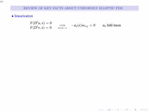
REVIEW OF KEY FACTS ABOUT UNIFORMLY ELLIPTIC PDE
• linearization
F(D2u, x) = 0F(D2v, x) = 0
=⇒w=u−v
−aij(x)wxixj = 0 aij bdd meas
122
REVIEW OF KEY FACTS ABOUT UNIFORMLY ELLIPTIC PDE
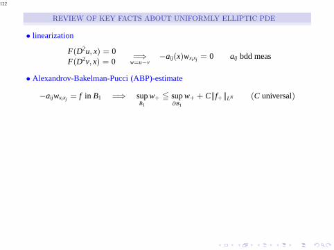
• linearization
F(D2u, x) = 0F(D2v, x) = 0
=⇒w=u−v
−aij(x)wxixj = 0 aij bdd meas
• Alexandrov-Bakelman-Pucci (ABP)-estimate
−aijwxixj = f in B1 =⇒ supB1
w+ ≦ sup∂B1
w+ + C‖f+‖LN (C universal)
123
REVIEW OF KEY FACTS ABOUT UNIFORMLY ELLIPTIC PDE
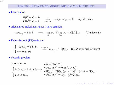
• linearization
F(D2u, x) = 0F(D2v, x) = 0
=⇒w=u−v
−aij(x)wxixj = 0 aij bdd meas
• Alexandrov-Bakelman-Pucci (ABP)-estimate
−aijwxixj = f in B1 =⇒ supB1
w+ ≦ sup∂B1
w+ + C‖f+‖LN (C universal)
• Fabes-Stroock (FS)-estimate(−aijwxixj = f in B1
w = 0 on∂B1
0<f<1=⇒ w|B1/2
≧ C‖f‖LM (C,M universal,M large)
• obstacle problem
u smallest st8
<
:
F(D2u, x) ≧ 0 in B1
u ≧ Q in B1
=⇒
• u = Q on∂B1
• F(D2u, x) = 0 in u > Q• 0≦ (u−Q)(y)≦C|x − y|2 (u(x) = Q(x))• F(D2u, x) = 1u=QF(Q, x)+
124
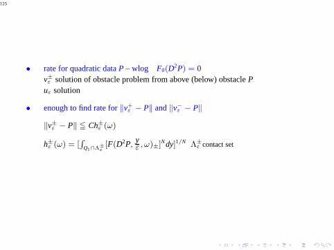
• rate for quadratic dataP – wlog F0(D2P) = 0v±ε solution of obstacle problem from above (below) obstaclePuε solution
125
• rate for quadratic dataP – wlog F0(D2P) = 0v±ε solution of obstacle problem from above (below) obstaclePuε solution
• enough to find rate for‖v+ε − P‖ and‖v−ε − P‖
‖v±ε − P‖ ≦ Ch±ε (ω)
h±ε (ω) = [
R
Q1∩Λ±ε
[F(D2P, yε , ω)±]Ndy]1/N Λ±
ε contact set
126
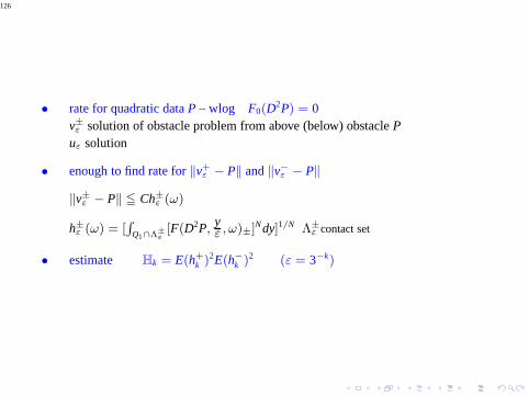
• rate for quadratic dataP – wlog F0(D2P) = 0v±ε solution of obstacle problem from above (below) obstaclePuε solution
• enough to find rate for‖v+ε − P‖ and‖v−ε − P‖
‖v±ε − P‖ ≦ Ch±ε (ω)
h±ε (ω) = [
R
Q1∩Λ±ε
[F(D2P, yε , ω)±]Ndy]1/N Λ±
ε contact set
• estimate Hk = E(h+k )2E(h−
k )2 (ε = 3−k)
127
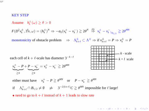
KEY STEP
Assume h±k (ω) ≥ θ > 0
F(D2v±k , 3kx, ω) = (h±
k )N ⇒ −aij(v+k − v−k ) ≧ 2θN FS
⇒ v+k − v−k |Q1/2
≧ 2θMN
monotonicityof obstacle problem ⇒ Λ±k+ℓ ⊂ Λ± ⇒ if v±k+ℓ = P ⇒ v±k = P
each cell ofk + ℓ-scale has diameter 3−k−ℓ
k - scale
k + l scale
v+k − P| z
≧0
+ P − v−k| z
≧0
= v+k − v−k ≧ 2θMN
either must have v+k − P ≧ θMN or P − v−k ≧ θMN
if Λ+k+ℓ ∩ B1/2 6= ∅ 6⇒ 3−2(k+ℓ)C ≧ θMN impossible forℓ large!
• need to go tok + ℓ instead ofk + 1 leads to slow rate


![DFT – Nuts & Bolts, Approximations [based on Chapter 3, Sholl & Steckel]](https://static.fdocument.org/doc/165x107/56814c92550346895db9a5ce/dft-nuts-bolts-approximations-based-on-chapter-3-sholl-steckel.jpg)