Rapid estimation of converted wave velocities using...
43
Rapid estimation of converted wave velocities using prestack migration John C. Bancroft, Thais Guirigay Helen Isaac 30 November, 2012 1
Transcript of Rapid estimation of converted wave velocities using...
Rapid estimation of converted wave velocities using prestack migration
John C. Bancroft, Thais Guirigay
Helen Isaac
30 November, 2012
1
0 500 1000 1500 2000 2500 30001
1.5
2
2.5
3
3.5
4
4.5
5
Depth (m)
Gam
ma γ
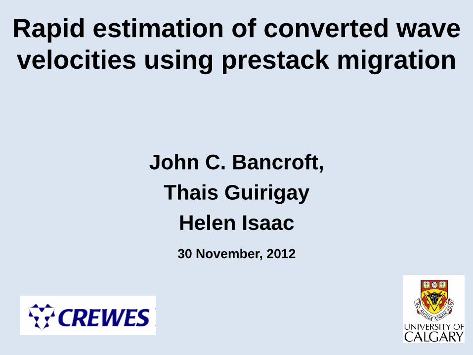
Gamma functions in depth from picked velocities
γ: Int. Vels. γ: RMS vels. γ: log
Motivation
2
Objectives Define a converted wave velocity Vc Use Vc to find Vs Create CCSP gathers
3
Outline • Objectives • Review EOM P-P and P-S, Vc • Estimating Vc • Estimation Vs • Formation of Gathers • Comments and Conclusion • Results next talk
4
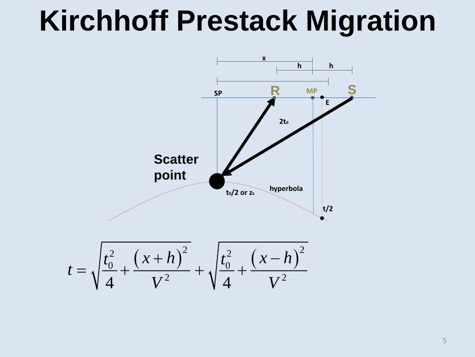
Scatter point
SP R S MP
t/2
t0/2 or z0 hyperbola
x h h
2te
( ) ( ) 2 20
2
2 22 20 0
2 24 42
4ex h x ht tt h
VVt
V+ −
= + + + +=
E
Kirchhoff Prestack Migration
5
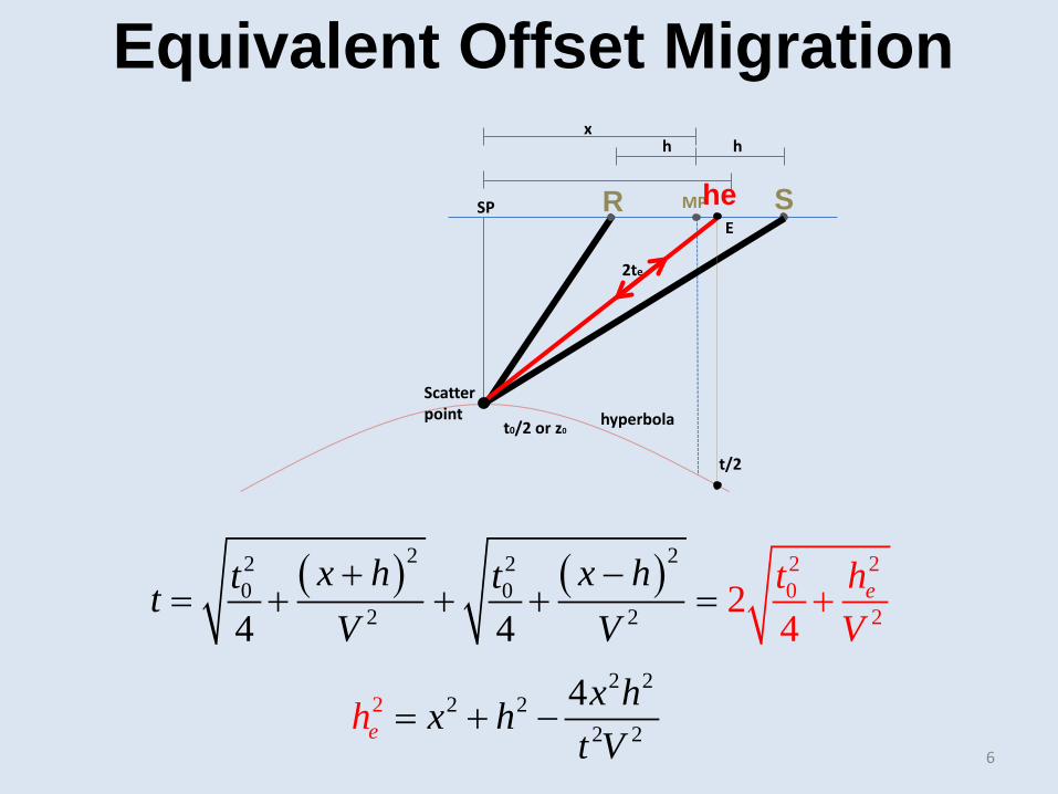
Equivalent Offset Migration
Scatter point
SP R S MP
t/2
t0/2 or z0 hyperbola
he
x h h
2te
( ) ( ) 2 20
2
2 22 20 0
2 24 42
4ex h x ht tt h
VVt
V+ −
= + + + +=
2 22 2 2
2 2
4eh x hx h
t V= + −
E
6
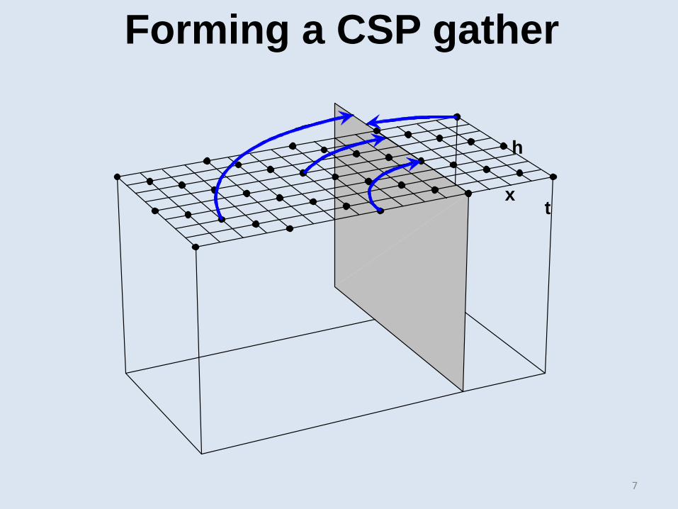
CMP or prestack migration gathe
h
t x
Forming a CSP gather
7
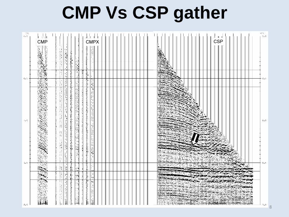
CMP Vs CSP gather
8
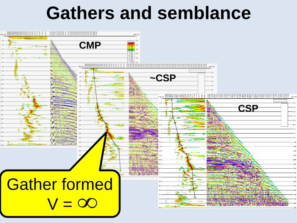
Gathers and semblance CMP
~CSP
CSP
Gather formed V = ∞
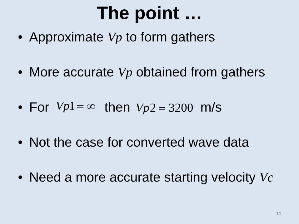
• Approximate Vp to form gathers
• More accurate Vp obtained from gathers
• For then m/s
• Not the case for converted wave data
• Need a more accurate starting velocity Vc
10
The point …
1Vp = ∞ 2 3200Vp =
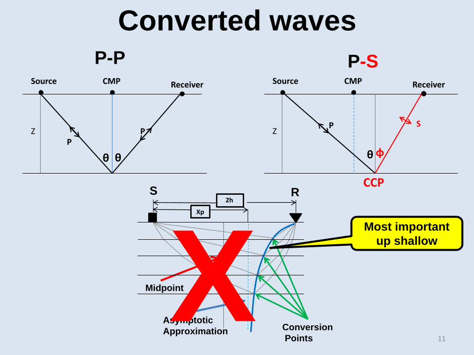
Converted waves
11
P-P Source Receiver CMP
Z P
P
θ θ
P-S Source Receiver CMP
CCP
θ φ
Z P S
S R
Conversion Points
Asymptotic Approximation
Midpoint
Xp
2h
Most important up shallow X
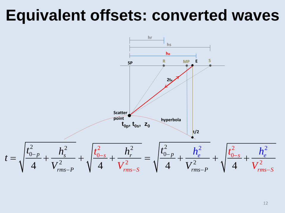
Equivalent offsets: converted waves hr
hs
2 20 0
2
2 22 20 0
2 2
2
2
2
4 4 4 4p ps r
rms P rms P
s s
rm S
e
s r
e
ms S
ht th ht tV V V
htV
− −
− − −
− −
−
= + + + = + + +
12
Scatter point
SP R S MP
t/2
hyperbola
he
2te
E
t0p, t0s, z0
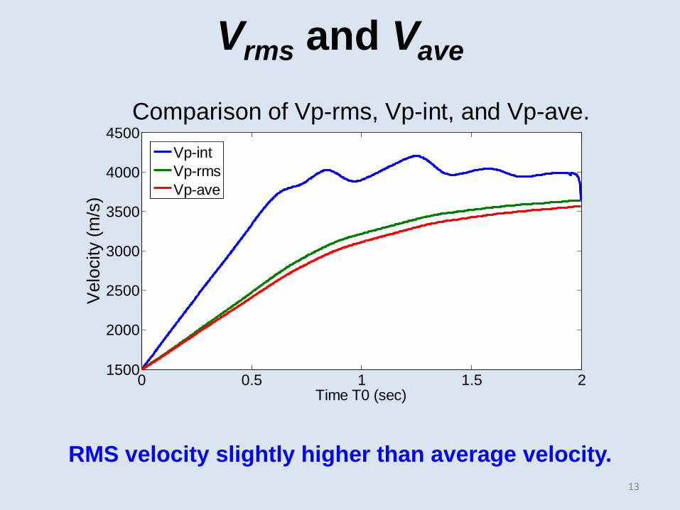
Vrms and Vave
0 0.5 1 1.5 21500
2000
2500
3000
3500
4000
4500
Time T0 (sec)
Vel
ocity
(m/s
)Comparison of Vp-rms, Vp-int, and Vp-ave.
Vp-intVp-rmsVp-ave
RMS velocity slightly higher than average velocity. 13
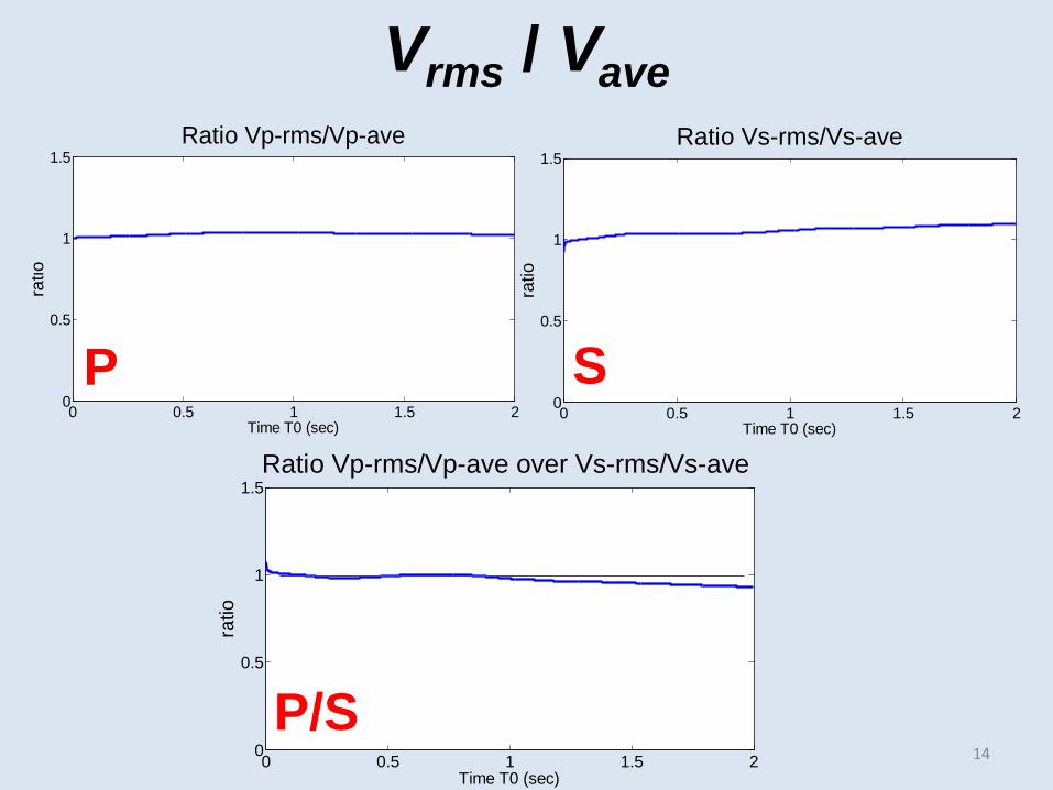
Vrms / Vave
0 0.5 1 1.5 20
0.5
1
1.5
Time T0 (sec)
ratio
Ratio Vp-rms/Vp-ave
P
0 0.5 1 1.5 20
0.5
1
1.5
Time T0 (sec)
ratio
Ratio Vp-rms/Vp-ave over Vs-rms/Vs-ave
P/S
0 0.5 1 1.5 20
0.5
1
1.5
Time T0 (sec)
ratio
Ratio Vs-rms/Vs-ave
S
14
2 2 2 2 20
2 2 20 00
1 1 1 ˆˆ ˆ ˆ1s r
rms p rms pe
rms s rme
s s
z hV V
t z h z hV
hV
z− −− −
= + + + +++=
2 20
2 ˆ ec
ztV
h+=
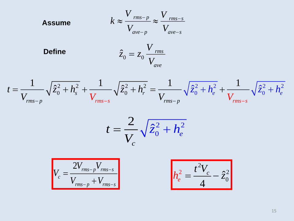
Assume rms p rms s
ave p ave s
V VkV V
− −
− −
≈ ≈
Define 0 0ˆ rms
ave
Vz zV
=
2220ˆ4
ceh t V z= −
2 rms p rms sc
rms p rms s
V VV
V V− −
− −
=+
15
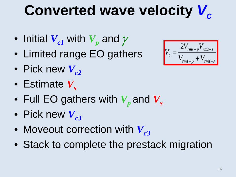
Converted wave velocity Vc
• Initial Vc1 with Vp and • Limited range EO gathers • Pick new Vc2
• Estimate Vs
• Full EO gathers with Vp and Vs • Pick new Vc3
• Moveout correction with Vc3 • Stack to complete the prestack migration
2 rms p rms sc
rms p rms s
V VV
V V− −
− −
=+
γ
16
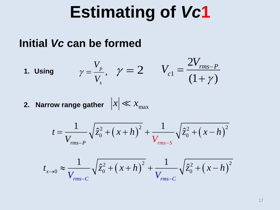
1. Using
2. Narrow range gather
Initial Vc can be formed
Estimating of Vc1
,p
s
VV
γ = 2γ =
maxx x
12(1 )
rms Pc
VVγ−=
+
( ) ( )2 22 20 0
1 1ˆ ˆrm rms Ss P
t z x h zV
x hV −−
= + + + + −
( ) ( )2 22 20 0 0
1 1ˆ ˆrms C m C
xr s
t z x hV V
z x h−
→−
≈ + + + + −
17
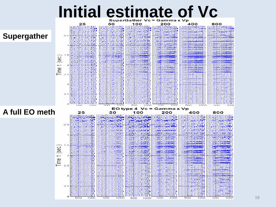
Supergather
A full EO method
Initial estimate of Vc
18
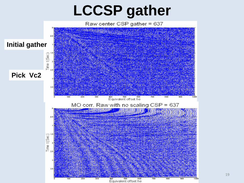
LCCSP gather
19
Initial gather
Pick Vc2
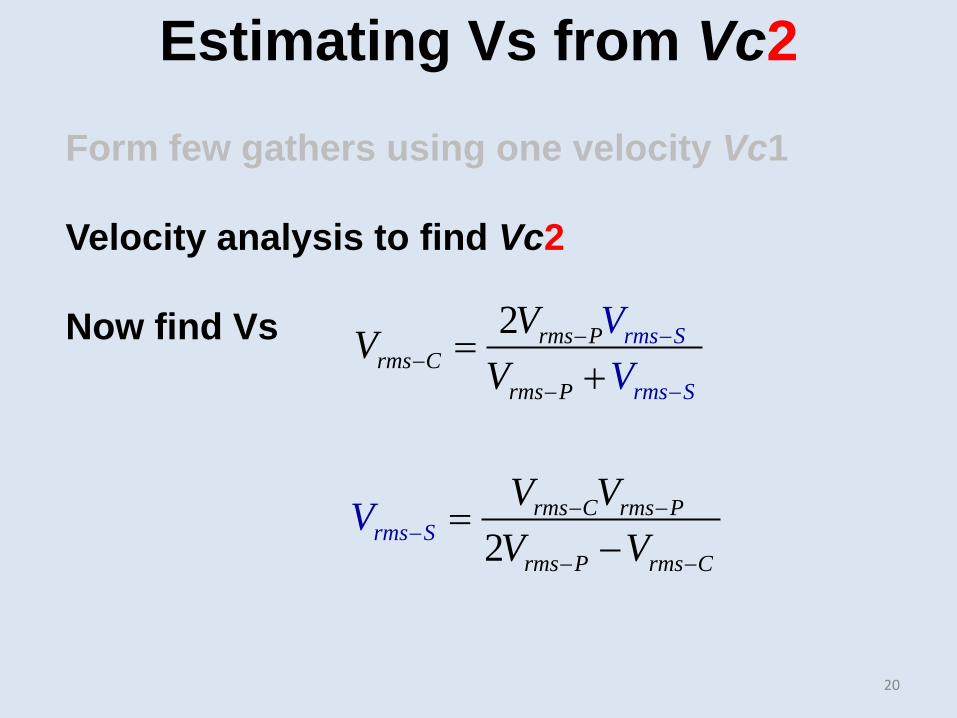
Form few gathers using one velocity Vc1 Velocity analysis to find Vc2 Now find Vs
Estimating Vs from Vc2
2 rms S
rms
rms Prms C
r s P Sm
VVV V
V −−−
− −
=+
2rms C rms
rmP
rms P rs S
ms C
V VV
VV
−
− −−
−=−
20
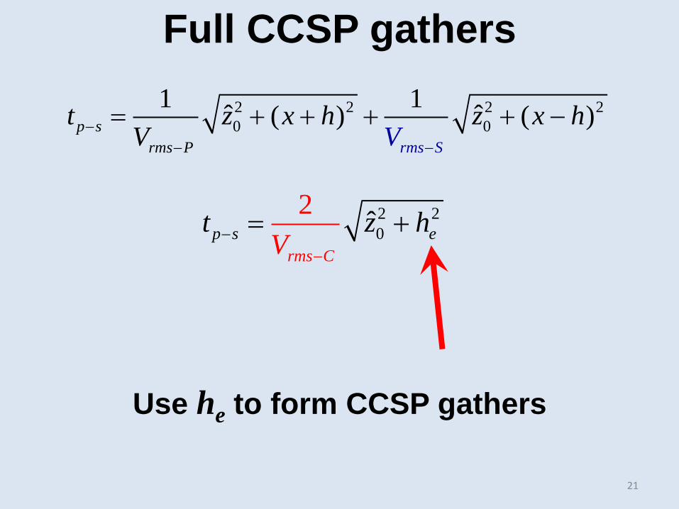
2 20
2 ˆrms C
p s et hV
z−
− = +
2 2 2 20 0
1 1ˆ ˆ( ) ( )rmsm S
p sr s P
t z x h z x hV V −
−−
= + + + + −
Full CCSP gathers
Use he to form CCSP gathers
21
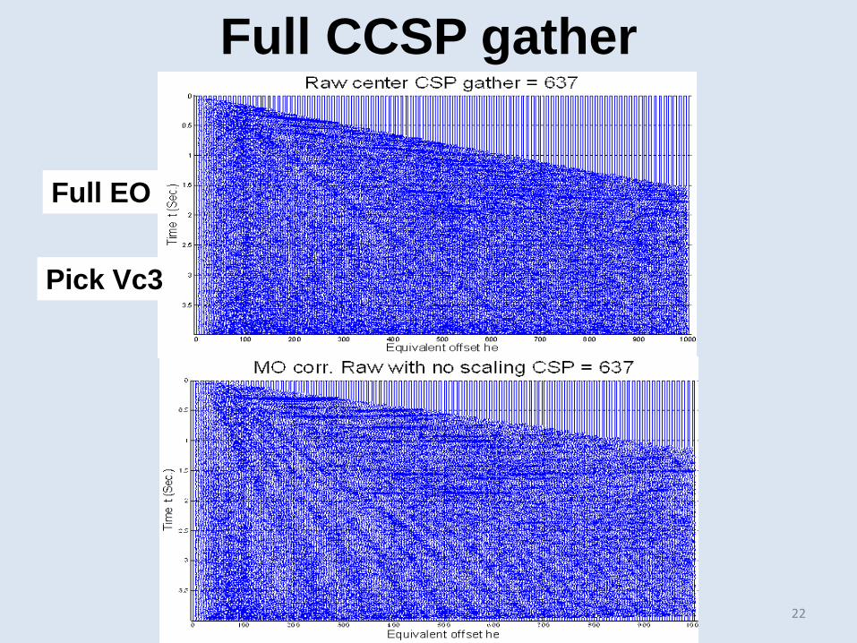
Full CCSP gather
22
Full EO
Pick Vc3
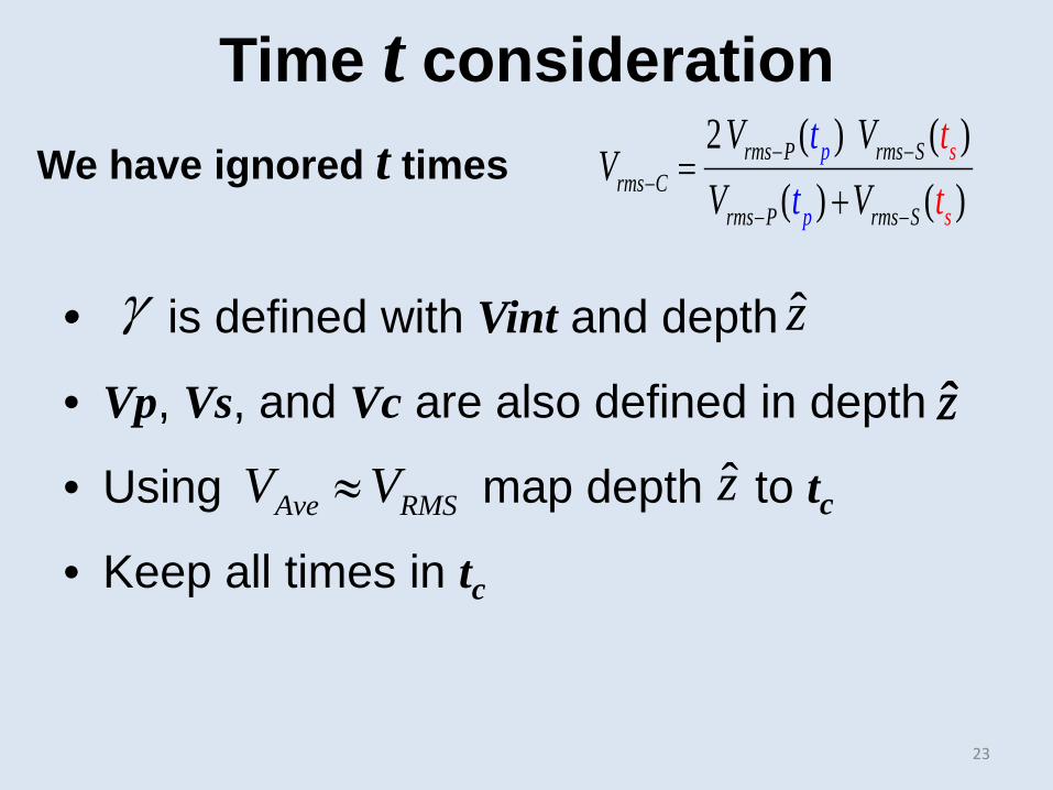
• is defined with Vint and depth
• Vp, Vs, and Vc are also defined in depth
• Using map depth to tc
• Keep all times in tc
We have ignored t times 2 ( ) ( )
( ) ( )srms P rms S
rms Cr
p
pP sms rms S
tV VV
tV Vt t
− −−
− −
=+
Time t consideration
γ
Ave RMSV V≈
z
zz
•
z
23
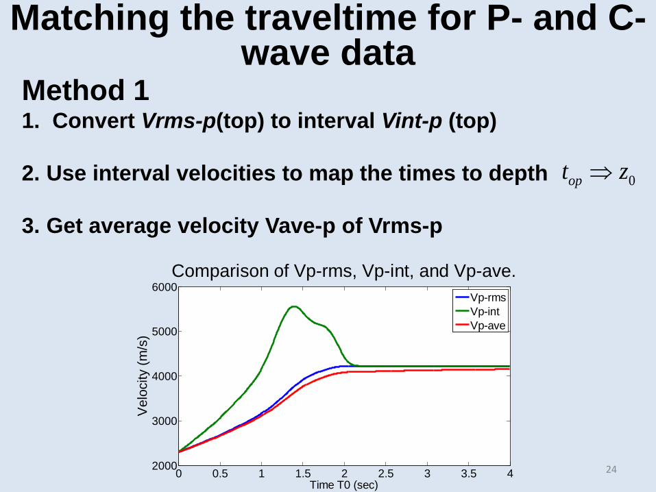
Matching the traveltime for P- and C-wave data
Method 1 1. Convert Vrms-p(top) to interval Vint-p (top)
2. Use interval velocities to map the times to depth
3. Get average velocity Vave-p of Vrms-p
0opt z⇒
0 0.5 1 1.5 2 2.5 3 3.5 42000
3000
4000
5000
6000
Time T0 (sec)
Vel
ocity
(m/s
)
Comparison of Vp-rms, Vp-int, and Vp-ave.
Vp-rmsVp-intVp-ave
24
Method 1 (continued) 4. Scale the amplitude Vint-c to Vint-p at z (same as top)
using 4. Use Vint-c (z) and the corresponding depth
increments, compute the C time at each depth.
5. Resample Vint-c from irregular times to equal time increments
6. Convert the interval C velocities to RMS C velocities
7. Get the depth of every Vc time sample using Vint-c
Matching the traveltime for P- and C-wave data
λ
25
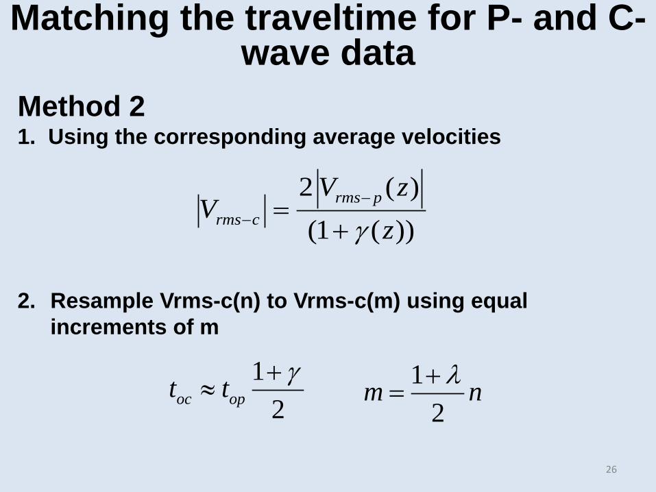
Matching the traveltime for P- and C-wave data
Method 2 1. Using the corresponding average velocities
2. Resample Vrms-c(n) to Vrms-c(m) using equal increments of m
2 ( )(1 ( ))
rms prms c
V zV
zγ−
− =+
12oc opt t γ+
≈ 12
m nλ+=
26
0 1 2 3 4 5 61500
2000
2500
3000
Time T0 (sec)
Vel
ocity
(m/s
)
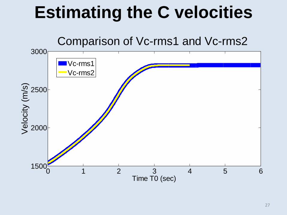
Comparison of Vc-rms1 and Vc-rms2
Vc-rms1Vc-rms2
Estimating the C velocities
27
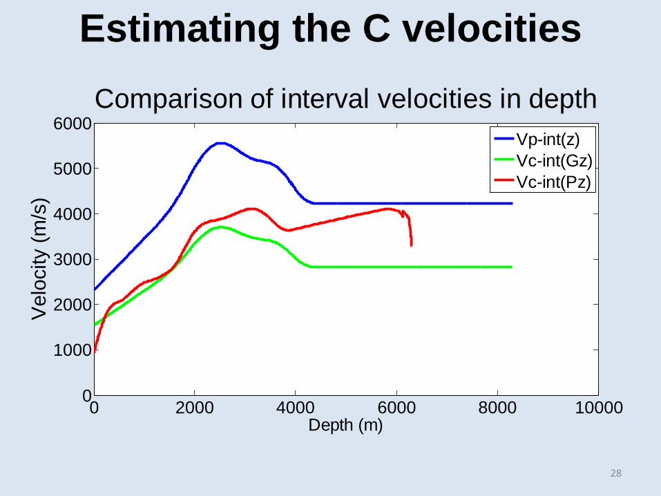
0 2000 4000 6000 8000 100000
1000
2000
3000
4000
5000
6000
Depth (m)
Vel
ocity
(m/s
)
Comparison of interval velocities in depth
Vp-int(z)Vc-int(Gz)Vc-int(Pz)
Estimating the C velocities
28
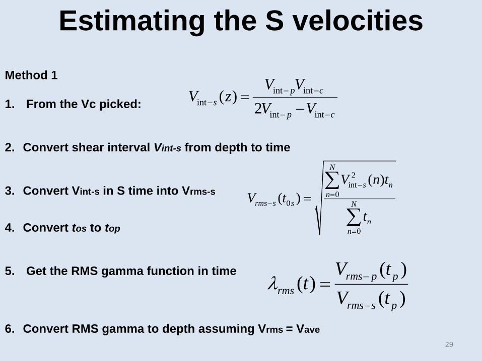
Method 1 1. From the Vc picked:
2. Convert shear interval Vint-s from depth to time
3. Convert Vint-s in S time into Vrms-s
4. Convert tos to top
5. Get the RMS gamma function in time
6. Convert RMS gamma to depth assuming Vrms = Vave
int intint
int int
( )2
p cs
p c
V VV z
V V− −
−− −
=−
2int
00
0
( )( )
N
s nn
rms s s N
nn
V n tV t
t
−=
−
=
=∑
∑
Estimating the S velocities
( )( )
( )rms p p
rmsrms s p
V tt
V tλ −
−
=
29
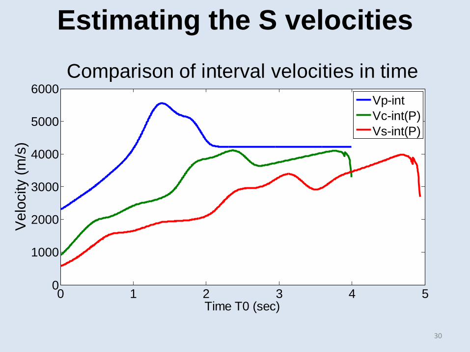
0 1 2 3 4 50
1000
2000
3000
4000
5000
6000
Time T0 (sec)
Vel
ocity
(m/s
)
Comparison of interval velocities in time
Vp-intVc-int(P)Vs-int(P)
Estimating the S velocities
30
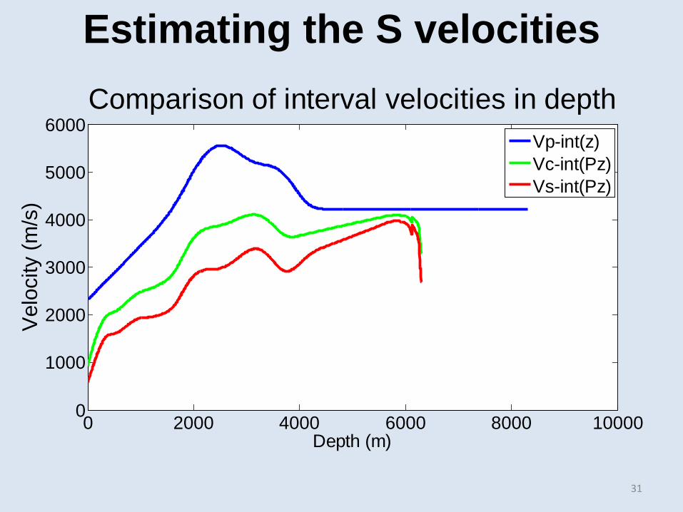
0 2000 4000 6000 8000 100000
1000
2000
3000
4000
5000
6000
Depth (m)
Vel
ocity
(m/s
)
Comparison of interval velocities in depth
Vp-int(z)Vc-int(Pz)Vs-int(Pz)
Estimating the S velocities
31
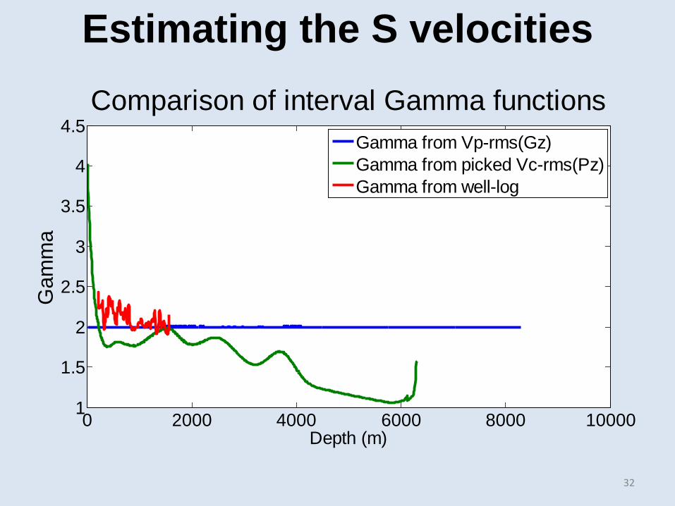
0 2000 4000 6000 8000 100001
1.5
2
2.5
3
3.5
4
4.5
Depth (m)
Gam
ma
Comparison of interval Gamma functions
Gamma from Vp-rms(Gz)Gamma from picked Vc-rms(Pz)Gamma from well-log
Estimating the S velocities
32
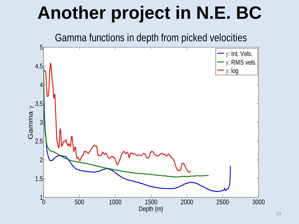
Another project in N.E. BC
0 500 1000 1500 2000 2500 30001
1.5
2
2.5
3
3.5
4
4.5
5
Depth (m)
Gam
ma γ
Gamma functions in depth from picked velocities
γ: Int. Vels. γ: RMS vels. γ: log
33
• Not yet • Next talk • Posters
Examples of data
34
• Use EO concepts to process P-S data • Need approximate velocity starting velocities
Vp and Vs • Can use a single velocity Vc most of the time • Simple process to estimate of Vc and Vs
– Vc1 from Vp and – Vc2 from initial gather – Vs from Vp and Vc2
• Produced reasonable values for
Comments and conclusions
γ
35
γ
γ
• Use EO concepts to process P-S data • Need approximate velocity starting velocities
Vp and Vs • Can use a single velocity Vc most of the time • Simple process to estimate of Vc and Vs
– Vc1 from Vp and – Vc2 from initial gather – Vs from Vp and Vc2
• Produced reasonable values for
Comments and conclusions
γ
36
γ
γ
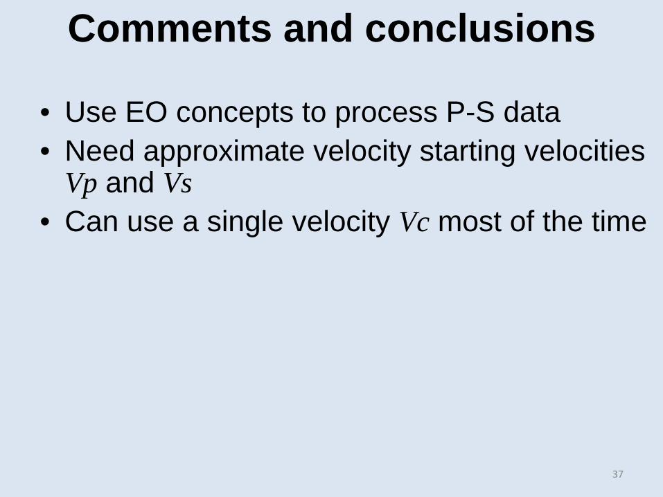
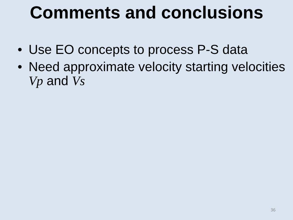
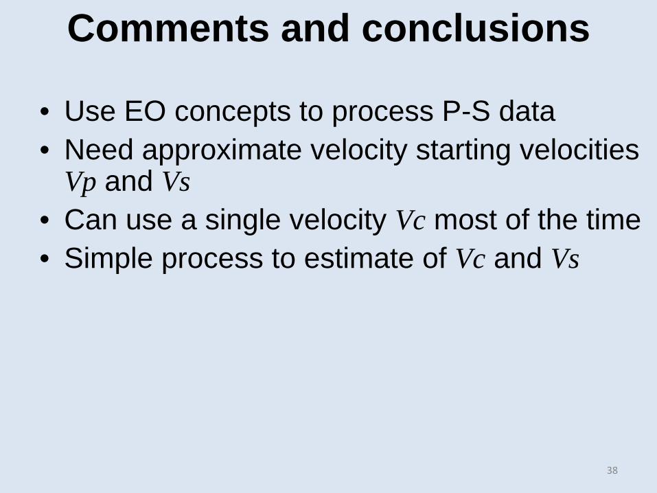
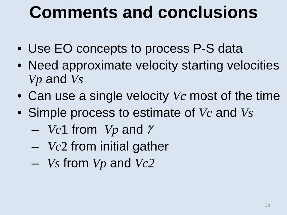
• Use EO concepts to process P-S data • Need approximate velocity starting velocities
Vp and Vs • Can use a single velocity Vc most of the time • Simple process to estimate of Vc and Vs
– Vc1 from Vp and – Vc2 from initial gather – Vs from Vp and Vc2
• Produced reasonable values for
Comments and conclusions
γ
37
γ
γ
• Use EO concepts to process P-S data • Need approximate velocity starting velocities
Vp and Vs • Can use a single velocity Vc most of the time • Simple process to estimate of Vc and Vs
– Vc1 from Vp and – Vc2 from initial gather – Vs from Vp and Vc2
• Produced reasonable values for
Comments and conclusions
γ
38
γ
γ
• Use EO concepts to process P-S data • Need approximate velocity starting velocities
Vp and Vs • Can use a single velocity Vc most of the time • Simple process to estimate of Vc and Vs
– Vc1 from Vp and – Vc2 from initial gather – Vs from Vp and Vc2
• Produced reasonable values for
Comments and conclusions
γ
39
γ
γ
• Use EO concepts to process P-S data • Need approximate velocity starting velocities
Vp and Vs • Can use a single velocity Vc most of the time • Simple process to estimate of Vc and Vs
– Vc1 from Vp and – Vc2 from initial gather – Vs from Vp and Vc2
• Produced reasonable values for
Comments and conclusions
γ
40
γ
γ
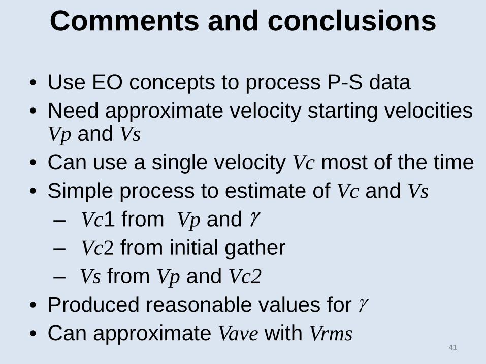
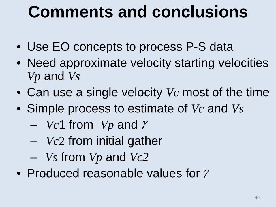
• Use EO concepts to process P-S data • Need approximate velocity starting velocities
Vp and Vs • Can use a single velocity Vc most of the time • Simple process to estimate of Vc and Vs
– Vc1 from Vp and – Vc2 from initial gather – Vs from Vp and Vc2
• Produced reasonable values for • Can approximate Vave with Vrms
Comments and conclusions
γ
41
γ
γ

Acknowledgments
All CREWES staff CREWES sponsors
42

Thanks 43