Ramanujan’s Most Singular Modulus - arXiv s Most Singular Modulus ... mathematicians who are...
44
arXiv:math/0308028v4 [math.HO] 17 Jul 2005 Ramanujan’s Most Singular Modulus MARK B. VILLARINO January 5, 2018 Abstract We present an elementary self-contained detailed computation of Ramanujan’s most famous singular modulus, k 210 , based on the Kronecker Limit Formula. Contents 1 The Singular Modulus α 2 1.1 Introduction .................................... 2 1.2 Singular moduli and units in quadratic fields .................. 3 1.3 Binary quadratic forms. The “numeri idonei” of Euler ............. 5 1.4 Elliptic modular functions and abelian extensions ............... 5 1.5 Prospectus ..................................... 7 2 Ramanujan’s Function F (α) 7 2.1 Complete elliptic integrals ............................ 7 2.2 The modular equation .............................. 8 2.3 Ramanujan’s theorem for α 2 , α 3 , and α 7 ................... 9 2.4 Ramanujan’s two-step algorithm ......................... 12 2.4.1 Ramanujan’s invariant g n ........................ 12 2.4.2 “a very curious algebraical lemma” ................... 13 2.4.3 The computation of α 30 ......................... 15 2.4.4 The computation of k 210 ......................... 16 3 Kronecker’s Limit Formula and the Computation of g 210 18 3.1 Binary quadratic forms .............................. 19 3.2 Kronecker’s limit formula ............................. 22 3.3 The relation with Ramanujan’s function g n ................... 24 3.4 The Kronecker–Weber computation of the weighted sum for m = 210 ... 26 3.5 The Dirichlet computation of the weighted sum ................ 29 3.5.1 The Dirichlet class number formulas .................. 33 3.5.2 The final computation of g 210 ...................... 33 1
-
Upload
nguyenthuan -
Category
Documents
-
view
224 -
download
1
Transcript of Ramanujan’s Most Singular Modulus - arXiv s Most Singular Modulus ... mathematicians who are...
arX
iv:m
ath/
0308
028v
4 [
mat
h.H
O]
17
Jul 2
005
Ramanujan’s Most Singular Modulus
MARK B. VILLARINO
January 5, 2018
Abstract
We present an elementary self-contained detailed computation of Ramanujan’s mostfamous singular modulus, k210, based on the Kronecker Limit Formula.
Contents
1 The Singular Modulus α 21.1 Introduction . . . . . . . . . . . . . . . . . . . . . . . . . . . . . . . . . . . . 21.2 Singular moduli and units in quadratic fields . . . . . . . . . . . . . . . . . . 31.3 Binary quadratic forms. The “numeri idonei” of Euler . . . . . . . . . . . . . 51.4 Elliptic modular functions and abelian extensions . . . . . . . . . . . . . . . 51.5 Prospectus . . . . . . . . . . . . . . . . . . . . . . . . . . . . . . . . . . . . . 7
2 Ramanujan’s Function F (α) 72.1 Complete elliptic integrals . . . . . . . . . . . . . . . . . . . . . . . . . . . . 72.2 The modular equation . . . . . . . . . . . . . . . . . . . . . . . . . . . . . . 82.3 Ramanujan’s theorem for α2, α3, and α7 . . . . . . . . . . . . . . . . . . . 92.4 Ramanujan’s two-step algorithm . . . . . . . . . . . . . . . . . . . . . . . . . 12
2.4.1 Ramanujan’s invariant gn . . . . . . . . . . . . . . . . . . . . . . . . 122.4.2 “a very curious algebraical lemma” . . . . . . . . . . . . . . . . . . . 132.4.3 The computation of α30 . . . . . . . . . . . . . . . . . . . . . . . . . 152.4.4 The computation of k210 . . . . . . . . . . . . . . . . . . . . . . . . . 16
3 Kronecker’s Limit Formula and the Computation of g210 183.1 Binary quadratic forms . . . . . . . . . . . . . . . . . . . . . . . . . . . . . . 193.2 Kronecker’s limit formula . . . . . . . . . . . . . . . . . . . . . . . . . . . . . 223.3 The relation with Ramanujan’s function gn . . . . . . . . . . . . . . . . . . . 243.4 The Kronecker–Weber computation of the weighted sum for m = 210 . . . 263.5 The Dirichlet computation of the weighted sum . . . . . . . . . . . . . . . . 29
3.5.1 The Dirichlet class number formulas . . . . . . . . . . . . . . . . . . 333.5.2 The final computation of g210 . . . . . . . . . . . . . . . . . . . . . . 33
1
3.6 Final comments . . . . . . . . . . . . . . . . . . . . . . . . . . . . . . . . . . 363.7 The miracle explained: Kronecker’s theory . . . . . . . . . . . . . . . . . . . 36
3.7.1 The first cancellation: Kronecker’s computation . . . . . . . . . . . . 373.7.2 The second cancellation: Dirichlet’s computation . . . . . . . . . . . 403.7.3 The general formula for gm where m is even . . . . . . . . . . . . . . 41
1 The Singular Modulus α
1.1 Introduction
In his second letter to G. H. Hardy, dated 27 February 1913, the self-taught Indian geniusSrinivasa Ramanujan announced the following outrageous theorem (numbered (17) inthe letter [17]):
THEOREM 1 (Ramanujan’s Singular Modulus). If
F (α) := 1 +
(
1
2
)2
α +
(
1·32·4
)2
α2 + · · · (1.1)
and
F (1− α) =√210 · F (α), (1.2)
then
α = (4−√15)4(8− 3
√7)2(2−
√3)2(6−
√35)2
· (√10− 3)4(
√7−
√6)4(
√15−
√14)2(
√2− 1)2.
(1.3)
(We have written α in place of Ramanujan’s k.)Our paper develops an elementary self-contained presentation of the history, theory and
algorithms for computing α as well as the details of its computation. Although (1.1)–(1.3)“...is one of Ramanujan’s most striking results,” (Hardy [13]), there is no published ab initio
account of it. Watson [18] published the only computation of α in the literature, but itpresupposes a considerable background knowledge on the part of the reader.
There always has been and continues to be a large population of students and practicingmathematicians who are intrigued by the folklore surrounding Ramanujan’s origins, whoare thrilled by the wondrous classical beauty of his mathematics, but who are put off bythe necessity of mastering multiple branches of advanced mathematics in order to be able toread the proofs.
We present for such readers an expository development of one of his most famous formu-lae, a detailed elementary self-contained connected account which takes an inquiring mind
2
with a modest background step-by-step to the full result. Our exposition thus contains his-torical information, motivational commentary, and offers a “cultural framework” as it were,so as to explain to the reader where the material “fits in” within the greater subject ofmathematics in general. It is far more than just a computation. It is a focused introductionto and an exposition of that specific area of mathematics which Ramanujan’s result sostrikingly illuminates.
Although our paper is expository, one hopes that the specialist can enjoy the point ofview and some novelties of detail. To begin with, our version of Ramanujan’s “very curiousalgebraical lemma” is new variant, and we use it for the major computations in our paper(see §2.4.2).
Moreover, our proof of Weber’s fundamental formula for g2n avoids Weber’s use of genustheory by appealing to an explicit composition formula for the quadratic form AX2 + BY 2
(see §3.7.1). This new approach simplifies the proof considerably and brings it within thereach of our target reader.
This reader needs to understand elementary analysis and algebra at the level of, say, threeyears at a university, as well as to be familiar with number theory to the level of quadraticreciprocity and the Jacobi symbol. All of this material is more than sufficiently covered inNiven and Zuckerman [16].
Much of the underlying general theory has been published inDavid Cox’s beautiful book[6] but he never deals with Ramanujan’s particular result. Finally, much of the material isin scattered references in several languages.
We call special attention to Volume 5 of Bruce Berndt’s edition of Ramanujan’sNotebooks [1], which devotes more than one hundred and fifty pages to the computation ofsingular moduli, and which is the most exhaustive reference on the subject. Unfortunately,although Berndt presents Chan’s proof of the “very curious algebraical lemma,” he does notdiscuss the complex computation of g210, the most difficult step, and thus is not a source forcomputing Ramanujan’s specific result. However, he does give some bibliographic references.
1.2 Singular moduli and units in quadratic fields
If we take Ramanujan’s theorem at face value and try to see if it makes sense (!) we canobserve from the definition:
F (α) := 1 +
(
1
2
)2
α +
(
1·32·4
)2
α2 + · · · (1.4)
that F (α) converges for −1 ≤ α < 1. Moreover, as α increases from 0 to 1, F (α) increasesfrom 1 to infinity and F (1− α) decreases from infinity to 1, and therefore
F (1− α)
F (α)
3
decreases monotonically from infinity to zero as α increases from 0 to 1. Thus there exists a
unique real number α with 0 < α < 1 such that
F (1− α)
F (α)=
√210. (1.5)
The numberk210 :=
√α ≡ √
α210
is called the singular modulus (for 210). If the right hand side of (1.2) is√n, n ∈ R+,
the same argument shows that there exists a unique real number αn with 0 ≤ αn < 1 whichsatisfies
F (1− αn)
F (αn)=
√n,
and we writekn :=
√αn.
and we call kn the singular modulus (for n). We use α and k without the subscript quitefrequently for ease of exposition. Its meaning should be clear from the context. Of course,what makes Ramanujan’s result (1.1)–(1.3) so astonishing is the explicit numerical value ofα210 as a finite product of the differences of quadratic surds. It is all the more amazing andunexpected since there is no evident a priori reason to expect such a value based on theexpansion (1.4). Where does α come from?
Let’s examine α, itself. In the first place, all the quadratic surds,
√15,
√7,√3,√35,
√10,
√6,√14,
√2
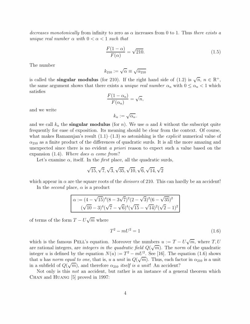
which appear in α are the square roots of the divisors of 210. This can hardly be an accident!In the second place, α is a product
α := (4−√15)4(8− 3
√7)2(2−
√3)2(6−
√35)2
(√10− 3)4(
√7−
√6)4(
√15−
√14)2(
√2− 1)2
of terms of the form T − U√m where
T 2 −mU2 = 1 (1.6)
which is the famous Pell’s equation. Moreover the numbers u := T − U√m, where T, U
are rational integers, are integers in the quadratic field Q(√m). The norm of the quadratic
integer u is defined by the equation N(u) := T 2 −mU2. See [16]. The equation (1.6) showsthat u has norm equal to one, that is, u a unit in Q(
√m). Thus, each factor in α210 is a unit
in a subfield of Q(√m), and therefore α210 itself is a unit ! An accident?
Not only is this not an accident, but rather is an instance of a general theorem whichChan and Huang [5] proved in 1997:
4
THEOREM 2 (Chan–Huang Unit Theorem). If n is of the form 4m + 2, then αn is
a unit.
We will call this result the Chan–Huang–UNIT–THEOREM, or “CHUT” for short. Infact, the CHUT deals with αn for any n, but this suffices for now.
The fact that α210 (and therefore k210) is a unit suggests that the explanation of itsvalue lies in the theory of quadratic number fields. But the theory of quadratic fields isa reformulation of the more classical theory of quadratic forms, and so we now turn todiscussing α in terms of this classical theory.
1.3 Binary quadratic forms. The “numeri idonei” of Euler
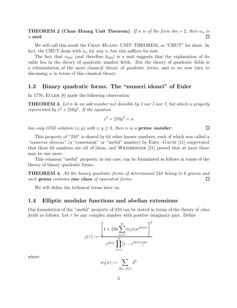
In 1776, Euler [8] made the following observation:
THEOREM 3. Let n be an odd number not divisible by 3 nor 5 nor 7, but which is properly
represented by x2 + 210y2. If the equation
x2 + 210y2 = n
has only ONE solution (x, y) with x, y ≥ 0, then n is a prime number.
This property of “210” is shared by 64 other known numbers, each of which was called a“numerus idoneus” (a “convenient” or “useful” number) by Euler. Gauss [11] conjecturedthat these 65 numbers are all of them, and Weinberger [21] proved that at most theremay be one more.
This common “useful” property, in our case, can be formulated as follows in terms of thetheory of binary quadratic forms:
THEOREM 4. All the binary quadratic forms of determinant 210 belong to 8 genera and
each genus contains one class of equivalent forms.
We will define the technical terms later on.
1.4 Elliptic modular functions and abelian extensions
Our formulation of the “useful” property of 210 can be stated in terms of the theory of classfields as follows. Let τ be any complex number with positive imaginary part. Define
j(τ) :=
[
1 + 240
∞∑
n=1
σ3(n)e2πinτ
]3
e2πiτ∞∏
n=1
[1− e2πinτ ]24
whereσ3(n) :=
∑
d|n, d≥1
d3
5
and “d|n” means “d divides n”.In the theory of elliptic functions (Borwein and Borwein [3]) one proves
j = 64(1− α + α2)3
α2(1− α)2(1.7)
where τ :=√−n, and α ≡ αn. (The reader should take note of the two uses of the letter
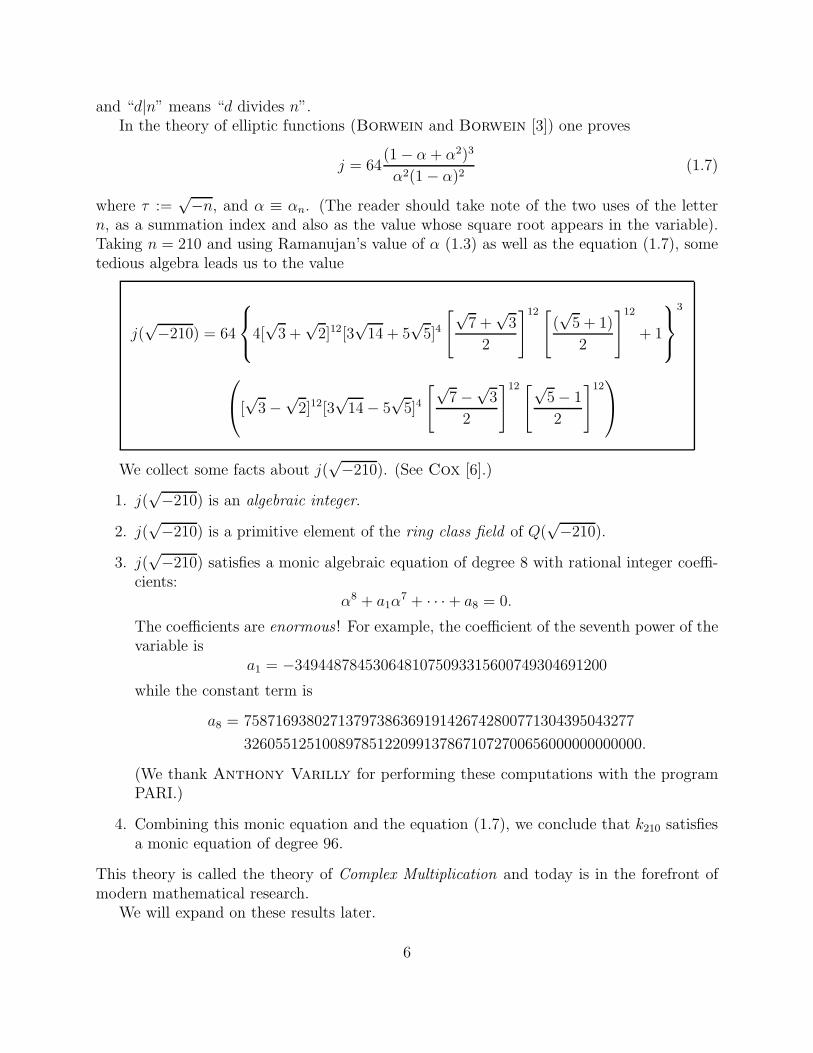
n, as a summation index and also as the value whose square root appears in the variable).Taking n = 210 and using Ramanujan’s value of α (1.3) as well as the equation (1.7), sometedious algebra leads us to the value
j(√−210) = 64
4[√3 +
√2]12[3
√14 + 5
√5]4
[√7 +
√3
2
]12 [
(√5 + 1)
2
]12
+ 1
3
[√3−
√2]12[3
√14− 5
√5]4
[√7−
√3
2
]12 [√5− 1
2
]12
We collect some facts about j(√−210). (See Cox [6].)
1. j(√−210) is an algebraic integer.
2. j(√−210) is a primitive element of the ring class field of Q(
√−210).
3. j(√−210) satisfies a monic algebraic equation of degree 8 with rational integer coeffi-
cients:α8 + a1α
7 + · · ·+ a8 = 0.
The coefficients are enormous ! For example, the coefficient of the seventh power of thevariable is
a1 = −3494487845306481075093315600749304691200
while the constant term is
a8 = 75871693802713797386369191426742800771304395043277
326055125100897851220991378671072700656000000000000.
(We thank Anthony Varilly for performing these computations with the programPARI.)
4. Combining this monic equation and the equation (1.7), we conclude that k210 satisfiesa monic equation of degree 96.
This theory is called the theory of Complex Multiplication and today is in the forefront ofmodern mathematical research.
We will expand on these results later.
6
1.5 Prospectus
Let’s stop to catch our breath. We’ve used several (as of yet) undefined technical terms andnotions. We’ve wandered over complex function theory, elementary and algebraic numbertheory, elliptic and modular functions, the genus theory of binary quadratic forms, andfinally, complex multiplication and class field theory (the theory of normal field extensionswith abelian Galois group)!
Did Ramanujan know any of this? Hardy [13] suggests that he most certainly did not
know the algebraic number theory, much less class field theory.Then how did he arrive at his results? Nobody knows, really, although Watson has made
a clever suggestion which we will not consider in this paper. (See [18] and [4]).Our paper presents an elementary method of computing α210.
1 It is based on the theoryof binary quadratic forms and uses the so-called Kronecker Limit Formula. We willdevelop the details in full since they have never been published. The fundamental sourcesare Weber’s treatise [19] and his paper [20]. In both references Weber simply states theresult of his computation, but suppresses the computation itself. Ramanujan uses the resultof Weber’s computation in order to compute α210, although he obtained it independently ofWeber. The fact is, nobody knows how he did it.
Our plan is the following: we will first develop the theory of the function F (α) and learnthe two-step algorithm which Ramanujan used. Then we will develop the theory of quadraticforms and the theory of Kronecker’s Limit Formula so as to be able to carry out the steps inRamanujan’s algorithm. Finally we will carry out the details of the computation and crownour memoir with an elementary and detailed demonstration of the general formula impliedby the computation which will explain a priori the miraculous computations we carry out.
2 Ramanujan’s Function F (α)
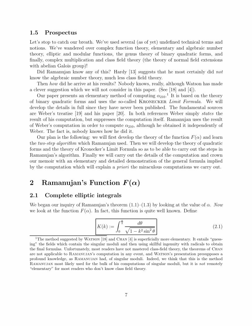
2.1 Complete elliptic integrals
We began our inquiry of Ramanujan’s theorem (1.1)–(1.3) by looking at the value of α. Nowwe look at the function F (α). In fact, this function is quite well known. Define
K(k) :=
∫ π
2
0
dθ√
1− k2 sin2 θ(2.1)
1The method suggested by Watson [18] and Chan [4] is superficially more elementary. It entails “guess-ing” the fields which contain the singular moduli and then using skillful ingenuity with radicals to obtainthe final formulas. Unfortunately, most readers have not mastered class-field theory, the theorems of Chan
are not applicable to Ramanujan’s computation in any event, and Watson’s presentation presupposes aprofound knowledge, as Ramanujan had, of singular moduli. Indeed, we think that this is the methodRamanujan most likely used for the bulk of his computations of singular moduli, but it is not remotely“elementary” for most readers who don’t know class field theory.
7
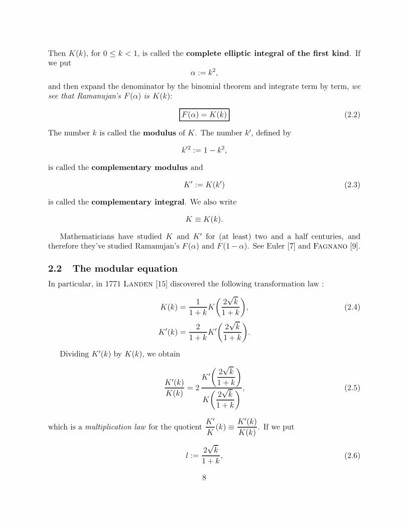
Then K(k), for 0 ≤ k < 1, is called the complete elliptic integral of the first kind. Ifwe put
α := k2,
and then expand the denominator by the binomial theorem and integrate term by term, wesee that Ramanujan’s F (α) is K(k):
F (α) = K(k) (2.2)
The number k is called the modulus of K. The number k′, defined by
k′2 := 1− k2,
is called the complementary modulus and
K ′ := K(k′) (2.3)
is called the complementary integral. We also write
K ≡ K(k).
Mathematicians have studied K and K ′ for (at least) two and a half centuries, andtherefore they’ve studied Ramanujan’s F (α) and F (1− α). See Euler [7] and Fagnano [9].
2.2 The modular equation
In particular, in 1771 Landen [15] discovered the following transformation law :
K(k) =1
1 + kK
(
2√k
1 + k
)
, (2.4)
K ′(k) =2
1 + kK ′(
2√k
1 + k
)
.
Dividing K ′(k) by K(k), we obtain
K ′(k)
K(k)= 2
K ′(
2√k
1 + k
)
K
(
2√k
1 + k
), (2.5)
which is a multiplication law for the quotientK ′
K(k) ≡ K ′(k)
K(k). If we put
l :=2√k
1 + k, (2.6)
8
the duplication law (2.5) takes the form
2L′
L=
K ′
K, (2.7)
where L′ and L are the complete elliptic integrals with respective moduli l′ and l. Theequation (2.6) can also be written
l2(1 + k)2 = 4k. (2.8)
Equations (2.6) and (2.8) are both called the modular equation of degree 2. The dupli-cation law (2.7) is one of an infinity of multiplication laws and each such law has a modularequation associated with it. We now make the following general definition.
DEFINITION 1. The modular equation of degree n is the algebraic equation
Ωn(k, l) = 0,
relating the moduli k and l for which the multiplication law
nL′
L=
K ′
K(2.9)
holds. Here K,K ′, L, L′ are the complete elliptic integrals with moduli k and l, and n > 0is a rational number.
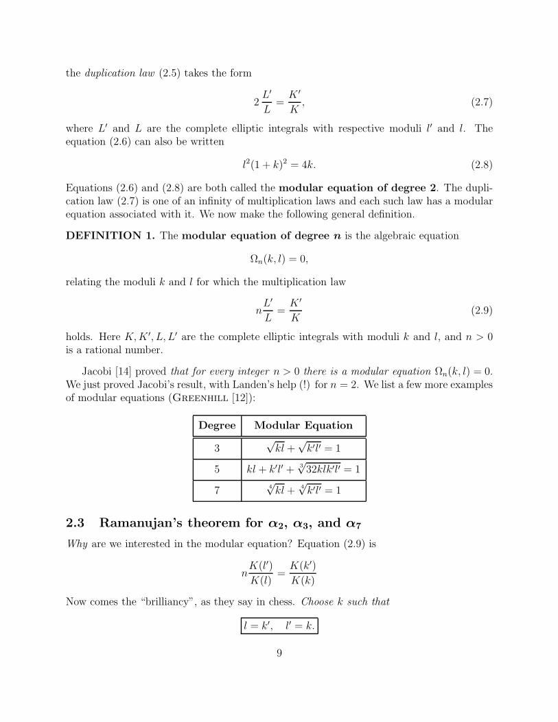
Jacobi [14] proved that for every integer n > 0 there is a modular equation Ωn(k, l) = 0.We just proved Jacobi’s result, with Landen’s help (!) for n = 2. We list a few more examplesof modular equations (Greenhill [12]):
Degree Modular Equation
3√kl +
√k′l′ = 1
5 kl + k′l′ + 3√32klk′l′ = 1
74√kl +
4√k′l′ = 1
2.3 Ramanujan’s theorem for α2, α3, and α7
Why are we interested in the modular equation? Equation (2.9) is
nK(l′)
K(l)=
K(k′)
K(k)
Now comes the “brilliancy”, as they say in chess. Choose k such that
l = k′, l′ = k.
9
Then (2.9) becomes
nK
K ′ =K ′
K,
or(K ′
K
)2
= n,
that is,K ′
K(k) =
√n. (2.10)
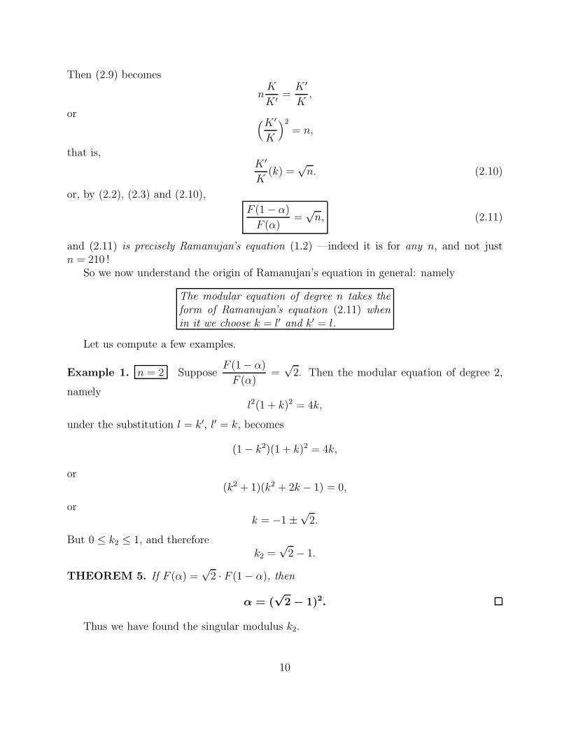
or, by (2.2), (2.3) and (2.10),
F (1− α)
F (α)=
√n, (2.11)
and (2.11) is precisely Ramanujan’s equation (1.2) —indeed it is for any n, and not justn = 210 !
So we now understand the origin of Ramanujan’s equation in general: namely
The modular equation of degree n takes the
form of Ramanujan’s equation (2.11) when
in it we choose k = l′ and k′ = l.
Let us compute a few examples.
Example 1. n = 2 SupposeF (1− α)
F (α)=
√2. Then the modular equation of degree 2,
namelyl2(1 + k)2 = 4k,
under the substitution l = k′, l′ = k, becomes
(1− k2)(1 + k)2 = 4k,
or(k2 + 1)(k2 + 2k − 1) = 0,
ork = −1 ±
√2.
But 0 ≤ k2 ≤ 1, and thereforek2 =
√2− 1.
THEOREM 5. If F (α) =√2 · F (1− α), then
α = (√
2 − 1)2.
Thus we have found the singular modulus k2.
10
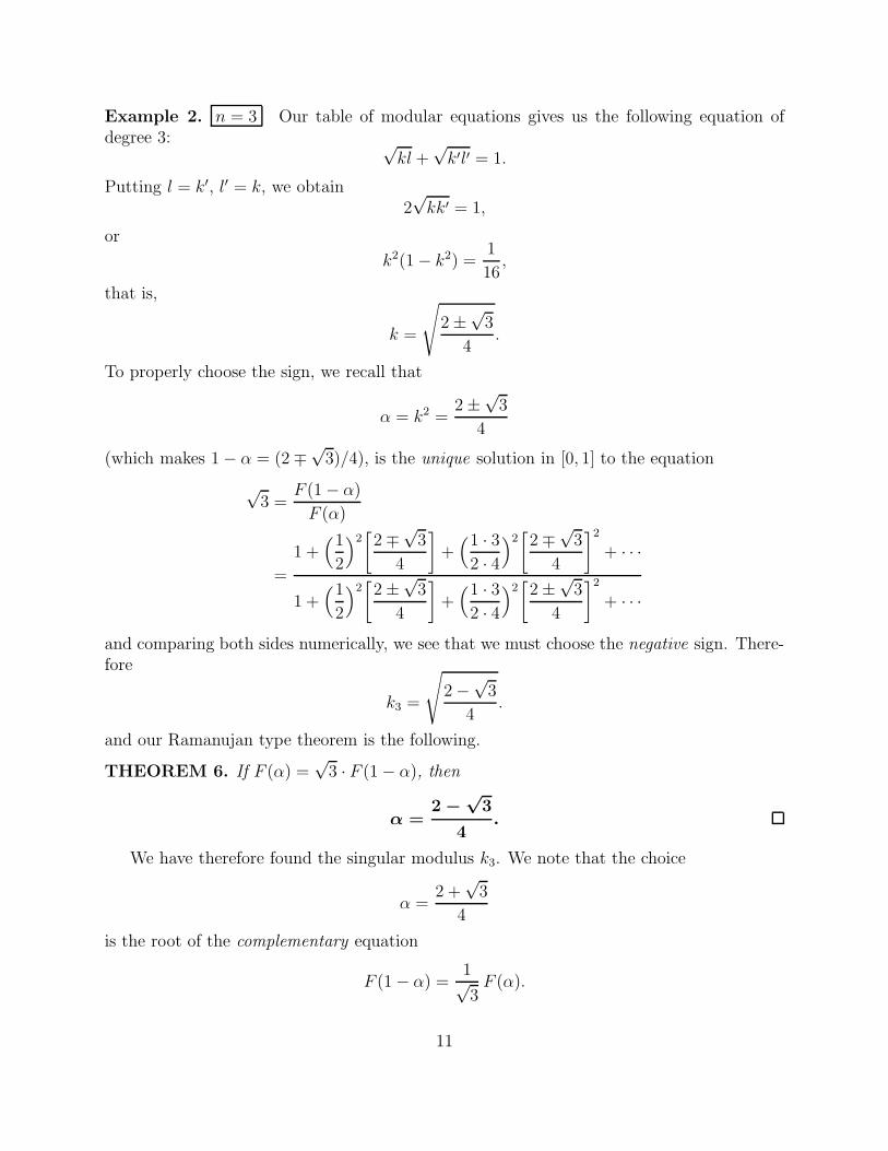
Example 2. n = 3 Our table of modular equations gives us the following equation ofdegree 3: √
kl +√k′l′ = 1.
Putting l = k′, l′ = k, we obtain2√kk′ = 1,
or
k2(1− k2) =1
16,
that is,
k =
√
2±√3
4.
To properly choose the sign, we recall that
α = k2 =2±
√3
4
(which makes 1− α = (2∓√3)/4), is the unique solution in [0, 1] to the equation
√3 =
F (1− α)
F (α)
=
1 +(1
2
)2[
2∓√3
4
]
+(1 · 32 · 4
)2[
2∓√3
4
]2
+ · · ·
1 +(1
2
)2[
2±√3
4
]
+(1 · 32 · 4
)2[
2±√3
4
]2
+ · · ·
and comparing both sides numerically, we see that we must choose the negative sign. There-fore
k3 =
√
2−√3
4.
and our Ramanujan type theorem is the following.
THEOREM 6. If F (α) =√3 · F (1− α), then
α =2 −
√3
4.
We have therefore found the singular modulus k3. We note that the choice
α =2 +
√3
4
is the root of the complementary equation
F (1− α) =1√3F (α).
11
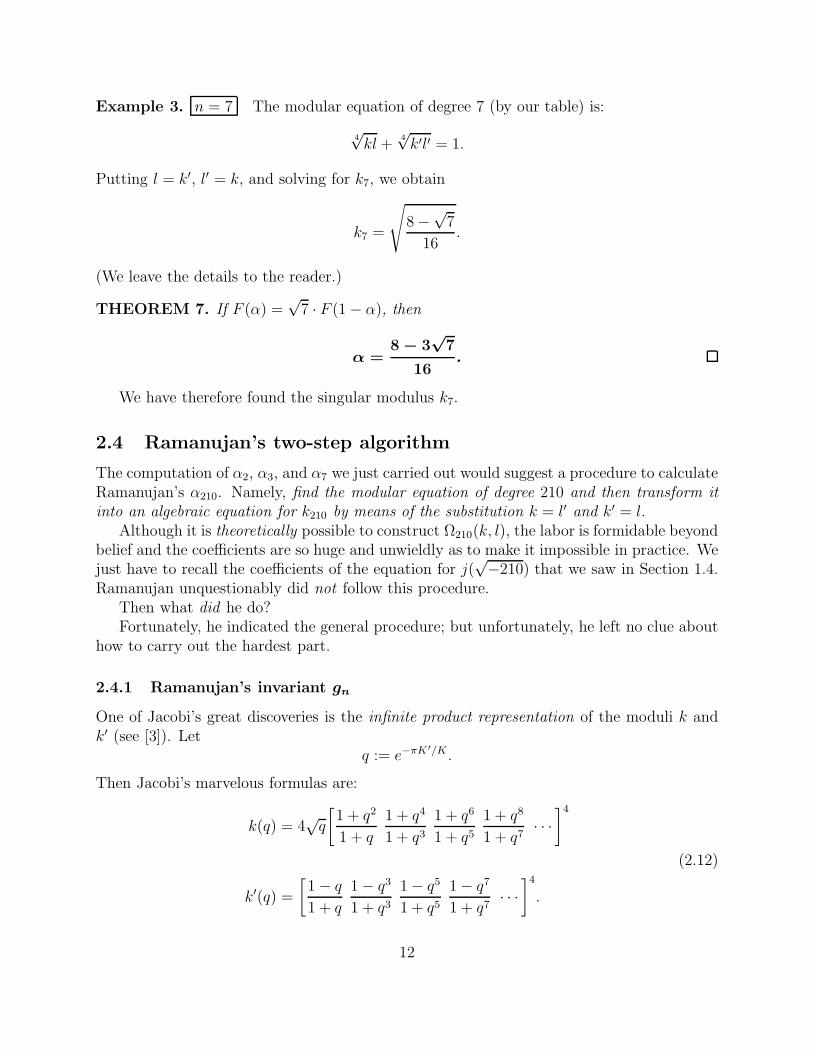
Example 3. n = 7 The modular equation of degree 7 (by our table) is:
4√kl +
4√k′l′ = 1.
Putting l = k′, l′ = k, and solving for k7, we obtain
k7 =
√
8−√7
16.
(We leave the details to the reader.)
THEOREM 7. If F (α) =√7 · F (1− α), then
α =8 − 3
√7
16.
We have therefore found the singular modulus k7.
2.4 Ramanujan’s two-step algorithm
The computation of α2, α3, and α7 we just carried out would suggest a procedure to calculateRamanujan’s α210. Namely, find the modular equation of degree 210 and then transform it
into an algebraic equation for k210 by means of the substitution k = l′ and k′ = l.Although it is theoretically possible to construct Ω210(k, l), the labor is formidable beyond
belief and the coefficients are so huge and unwieldly as to make it impossible in practice. Wejust have to recall the coefficients of the equation for j(
√−210) that we saw in Section 1.4.
Ramanujan unquestionably did not follow this procedure.Then what did he do?Fortunately, he indicated the general procedure; but unfortunately, he left no clue about
how to carry out the hardest part.
2.4.1 Ramanujan’s invariant gn
One of Jacobi’s great discoveries is the infinite product representation of the moduli k andk′ (see [3]). Let
q := e−πK ′/K .
Then Jacobi’s marvelous formulas are:
k(q) = 4√q
[
1 + q2
1 + q
1 + q4
1 + q31 + q6
1 + q51 + q8
1 + q7· · ·]4
k′(q) =
[
1− q
1 + q
1− q3
1 + q31− q5
1 + q51− q7
1 + q7· · ·]4
.
(2.12)
12
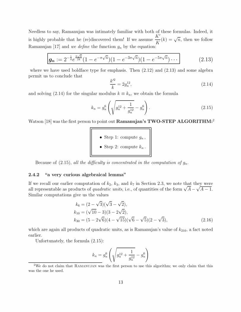
Needless to say, Ramanujan was intimately familiar with both of these formulas. Indeed, it
is highly probable that he (re)discovered them! If we assumeK ′
K(k) =
√n, then we follow
Ramanujan [17] and we define the function gn by the equation:
gn := 2−1
4eπ
√
n
24 (1− e−π√n)(1− e−3π
√n)(1− e−5π
√n) · · · (2.13)
where we have used boldface type for emphasis. Then (2.12) and (2.13) and some algebrapermit us to conclude that
k′2
k= 2g12n , (2.14)
and solving (2.14) for the singular modulus k ≡ kn, we obtain the formula
kn = g6n
(√
g12n +1
g12n− g6n
)
. (2.15)
Watson [18] was the first person to point outRamanujan’s TWO-STEP ALGORITHM:2
• Step 1: compute gn ,
• Step 2: compute kn .
Because of (2.15), all the difficulty is concentrated in the computation of gn.
2.4.2 “a very curious algebraical lemma”
If we recall our earlier computation of k2, k3, and k7 in Section 2.3, we note that they wereall representable as products of quadratic units, i.e., of quantities of the form
√A−
√A− 1.
Similar computations give us the values
k6 = (2−√3)(
√3−
√2),
k10 = (√10− 3)(3− 2
√2),
k30 = (5− 2√6)(4−
√15)(
√6−
√5)(2−
√3), (2.16)
which are again all products of quadratic units, as is Ramanujan’s value of k210, a fact notedearlier.
Unfortunately, the formula (2.15):
kn = g6n
(√
g12n +1
g12n− g6n
)
2We do not claim that Ramanujan was the first person to use this algorithm; we only claim that thiswas the one he used.
13
does not easily transform itself into a product of quadratic units. Perhaps the reader wouldlike to try to transform (2.15) into (2.16) by using the value
g630 = (3 +√10)(2 +
√5).
Observe that g30 is a product of units. The same is true of all gn used by Ramanujan.Writing (2.14) in the form
1
k− k = 2g12n , (2.17)
we see that Ramanujan had to solve the quadratic equation (2.17), in which gn is a productof units, and then express the root kn again as a product of units.
We now quote Hardy [13]:
“This result Ramanujan [achieved], granted thevalue of [gn], by a very curious algebraical lemma.”
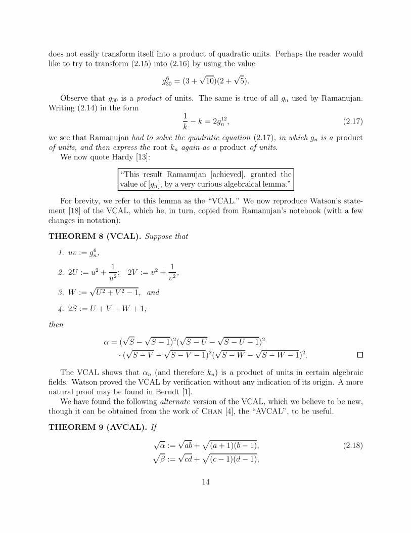
For brevity, we refer to this lemma as the “VCAL.” We now reproduce Watson’s state-ment [18] of the VCAL, which he, in turn, copied from Ramanujan’s notebook (with a fewchanges in notation):
THEOREM 8 (VCAL). Suppose that
1. uv := g6n,
2. 2U := u2 +1
u2; 2V := v2 +
1
v2,
3. W :=√U2 + V 2 − 1, and
4. 2S := U + V +W + 1;
then
α = (√S −
√S − 1)2(
√S − U −
√S − U − 1)2
· (√S − V −
√S − V − 1)2(
√S −W −
√S −W − 1)2.
The VCAL shows that αn (and therefore kn) is a product of units in certain algebraicfields. Watson proved the VCAL by verification without any indication of its origin. A morenatural proof may be found in Berndt [1].
We have found the following alternate version of the VCAL, which we believe to be new,though it can be obtained from the work of Chan [4], the “AVCAL”, to be useful.
THEOREM 9 (AVCAL). If
√α :=
√ab+
√
(a+ 1)(b− 1), (2.18)√
β :=√cd+
√
(c− 1)(d− 1),
14
then
x1 := (√a+ 1−
√a)(
√b−
√b− 1)(
√c−
√c− 1)(
√d−
√d− 1),
x2 := −(√a+ 1 +
√a)(
√b+
√b− 1)(
√c +
√c− 1)(
√d+
√d− 1)
are the roots of1
x− x = 2
[√
αβ +√
(α + 1)(β − 1)]
.
The proof is quite simple. We offer the following two examples.
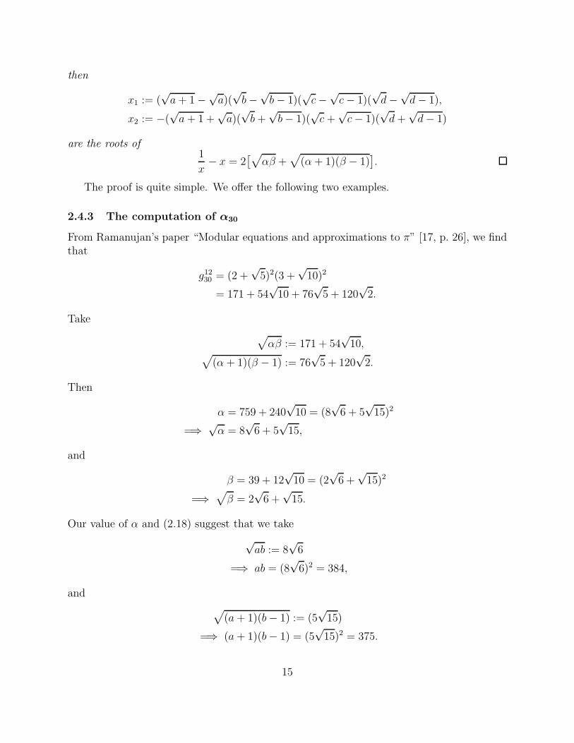
2.4.3 The computation of α30
From Ramanujan’s paper “Modular equations and approximations to π” [17, p. 26], we findthat
g1230 = (2 +√5)2(3 +
√10)2
= 171 + 54√10 + 76
√5 + 120
√2.
Take
√
αβ := 171 + 54√10,
√
(α + 1)(β − 1) := 76√5 + 120
√2.
Then
α = 759 + 240√10 = (8
√6 + 5
√15)2
=⇒√α = 8
√6 + 5
√15,
and
β = 39 + 12√10 = (2
√6 +
√15)2
=⇒√
β = 2√6 +
√15.
Our value of α and (2.18) suggest that we take
√ab := 8
√6
=⇒ ab = (8√6)2 = 384,
and
√
(a+ 1)(b− 1) := (5√15)
=⇒ (a+ 1)(b− 1) = (5√15)2 = 375.
15
Solving for a and b, we obtaina = 24, b = 16.
Similarly,cd = 24, (c− 1)(d− 1) = 15,
and thereforec = 6, d = 4.
Since 0 ≤ α < 1, we conclude from the AVCAL that
k30 = (5− 2√6)(4−
√15)(
√6−
√5)(2−
√3)
as given in Berndt’s paper “Ramanujan’s singular moduli” [2, Thm. 2.1].
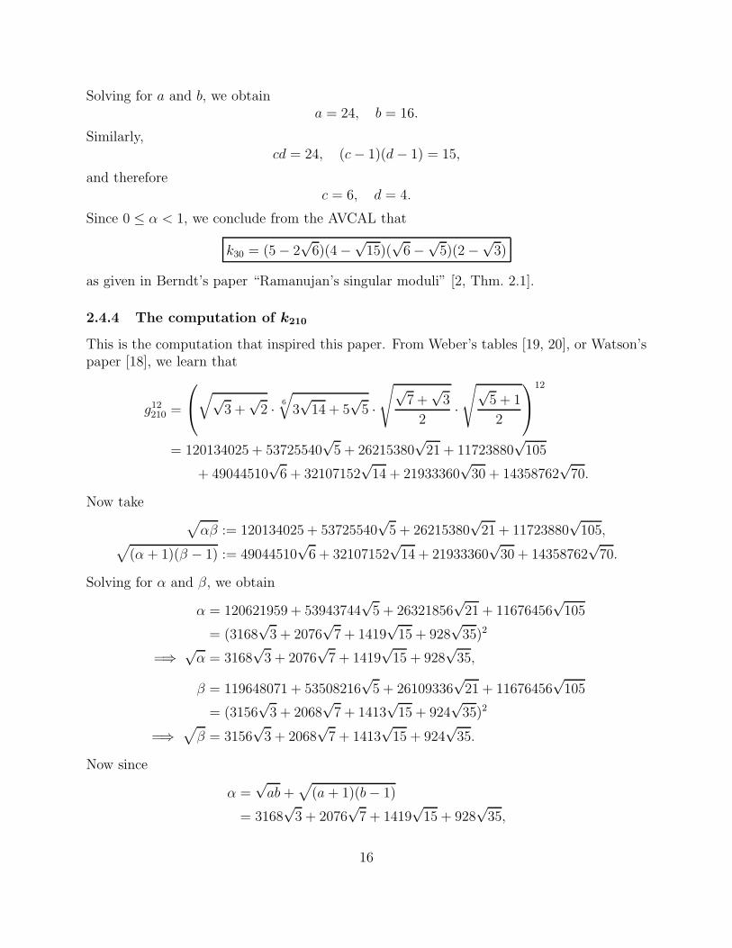
2.4.4 The computation of k210
This is the computation that inspired this paper. From Weber’s tables [19, 20], or Watson’spaper [18], we learn that
g12210 =
√√3 +
√2 · 6
√
3√14 + 5
√5 ·
√√7 +
√3
2·
√√5 + 1
2
12
= 120134025 + 53725540√5 + 26215380
√21 + 11723880
√105
+ 49044510√6 + 32107152
√14 + 21933360
√30 + 14358762
√70.
Now take√
αβ := 120134025 + 53725540√5 + 26215380
√21 + 11723880
√105,
√
(α + 1)(β − 1) := 49044510√6 + 32107152
√14 + 21933360
√30 + 14358762
√70.
Solving for α and β, we obtain
α = 120621959 + 53943744√5 + 26321856
√21 + 11676456
√105
= (3168√3 + 2076
√7 + 1419
√15 + 928
√35)2
=⇒√α = 3168
√3 + 2076
√7 + 1419
√15 + 928
√35,
β = 119648071 + 53508216√5 + 26109336
√21 + 11676456
√105
= (3156√3 + 2068
√7 + 1413
√15 + 924
√35)2
=⇒√
β = 3156√3 + 2068
√7 + 1413
√15 + 924
√35.
Now since
α =√ab+
√
(a + 1)(b− 1)
= 3168√3 + 2076
√7 + 1419
√15 + 928
√35,
16
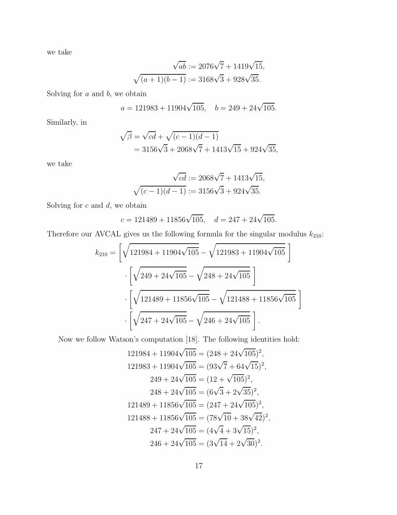
we take√ab := 2076
√7 + 1419
√15,
√
(a+ 1)(b− 1) := 3168√3 + 928
√35.
Solving for a and b, we obtain
a = 121983 + 11904√105, b = 249 + 24
√105.
Similarly, in√
β =√cd+
√
(c− 1)(d− 1)
= 3156√3 + 2068
√7 + 1413
√15 + 924
√35,
we take√cd := 2068
√7 + 1413
√15,
√
(c− 1)(d− 1) := 3156√3 + 924
√35.
Solving for c and d, we obtain
c = 121489 + 11856√105, d = 247 + 24
√105.
Therefore our AVCAL gives us the following formula for the singular modulus k210:
k210 =
[√
121984 + 11904√105−
√
121983 + 11904√105
]
·[√
249 + 24√105−
√
248 + 24√105
]
·[√
121489 + 11856√105−
√
121488 + 11856√105
]
·[√
247 + 24√105−
√
246 + 24√105
]
.
Now we follow Watson’s computation [18]. The following identities hold:
121984 + 11904√105 = (248 + 24
√105)2,
121983 + 11904√105 = (93
√7 + 64
√15)2,
249 + 24√105 = (12 +
√105)2,
248 + 24√105 = (6
√3 + 2
√35)2,
121489 + 11856√105 = (247 + 24
√105)2,
121488 + 11856√105 = (78
√10 + 38
√42)2,
247 + 24√105 = (4
√4 + 3
√15)2,
246 + 24√105 = (3
√14 + 2
√30)2.
17
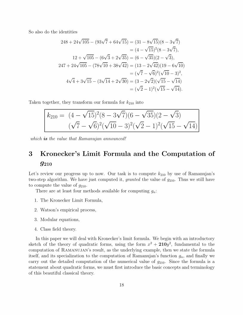
So also do the identities
248 + 24√105− (93
√7 + 64
√15) = (31− 8
√15)(8− 3
√7)
= (4−√15)2(8− 3
√7),
12 +√105− (6
√3 + 2
√35) = (6−
√35)(2−
√3),
247 + 24√105− (78
√10 + 38
√42) = (13− 2
√42)(19− 6
√10)
= (√7−
√6)2(
√10− 3)2,
4√4 + 3
√15− (3
√14 + 2
√30) = (3− 2
√2)(
√15−
√14)
= (√2− 1)2(
√15−
√14).
Taken together, they transform our formula for k210 into
k210 = (4−√15)2(8− 3
√7)(6−
√35)(2−
√3)
(√7−
√6)2(
√10− 3)2(
√2− 1)2(
√15−
√14)
which is the value that Ramanujan announced!
3 Kronecker’s Limit Formula and the Computation of
g210
Let’s review our progress up to now. Our task is to compute k210 by use of Ramanujan’stwo-step algorithm. We have just computed it, granted the value of g210. Thus we still haveto compute the value of g210.
There are at least four methods available for computing gn:
1. The Kronecker Limit Formula,
2. Watson’s empirical process,
3. Modular equations,
4. Class field theory.
In this paper we will deal with Kronecker’s limit formula. We begin with an introductorysketch of the theory of quadratic forms, using the form x2 + 210y2, fundamental to thecomputation of Ramanujan’s result, as the underlying example, then we state the formulaitself, and its specialization to the computation of Ramanujan’s function gn, and finally wecarry out the detailed computation of the numerical value of g210. Since the formula is astatement about quadratic forms, we must first introduce the basic concepts and terminologyof this beautiful classical theory.
18
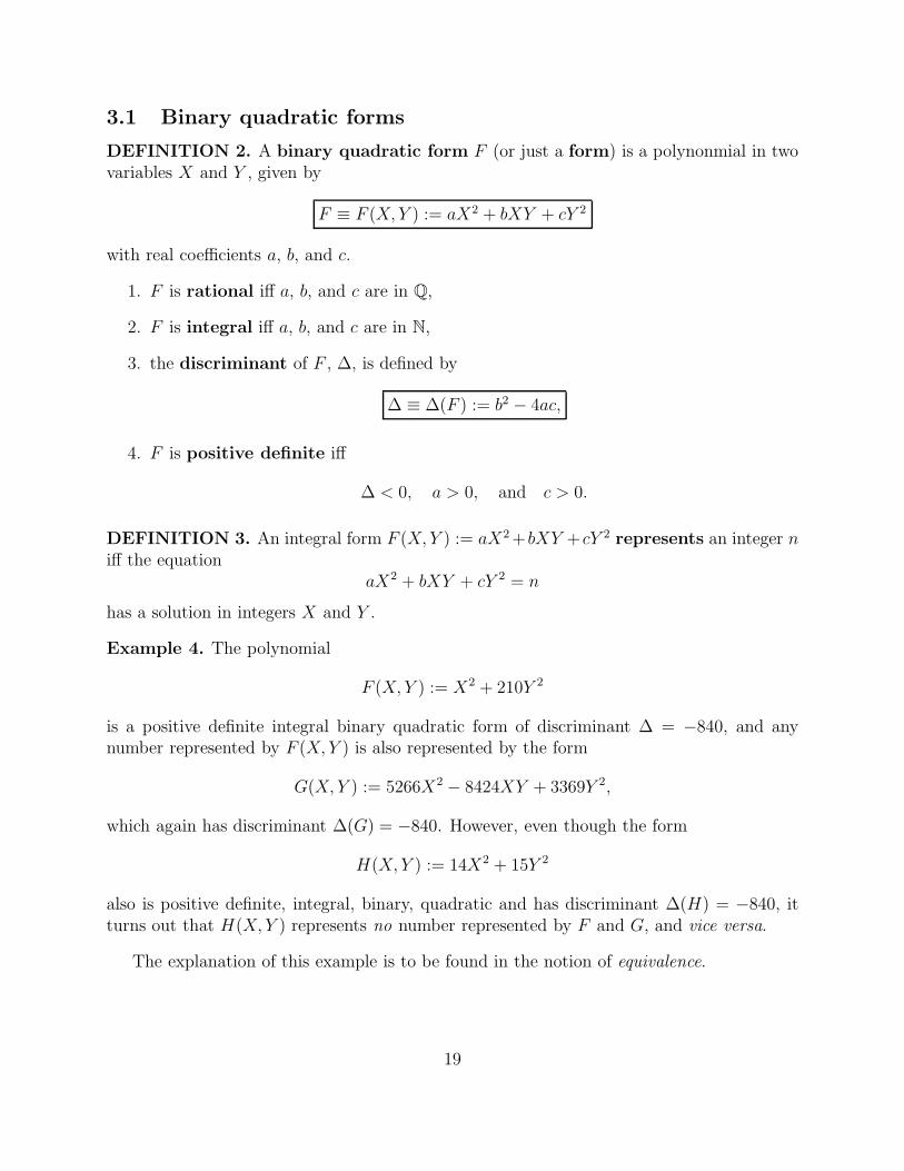
3.1 Binary quadratic forms
DEFINITION 2. A binary quadratic form F (or just a form) is a polynonmial in twovariables X and Y , given by
F ≡ F (X, Y ) := aX2 + bXY + cY 2
with real coefficients a, b, and c.
1. F is rational iff a, b, and c are in Q,
2. F is integral iff a, b, and c are in N,
3. the discriminant of F , ∆, is defined by
∆ ≡ ∆(F ) := b2 − 4ac,
4. F is positive definite iff
∆ < 0, a > 0, and c > 0.
DEFINITION 3. An integral form F (X, Y ) := aX2+bXY +cY 2 represents an integer niff the equation
aX2 + bXY + cY 2 = n
has a solution in integers X and Y .
Example 4. The polynomial
F (X, Y ) := X2 + 210Y 2
is a positive definite integral binary quadratic form of discriminant ∆ = −840, and anynumber represented by F (X, Y ) is also represented by the form
G(X, Y ) := 5266X2 − 8424XY + 3369Y 2,
which again has discriminant ∆(G) = −840. However, even though the form
H(X, Y ) := 14X2 + 15Y 2
also is positive definite, integral, binary, quadratic and has discriminant ∆(H) = −840, itturns out that H(X, Y ) represents no number represented by F and G, and vice versa.
The explanation of this example is to be found in the notion of equivalence.
19
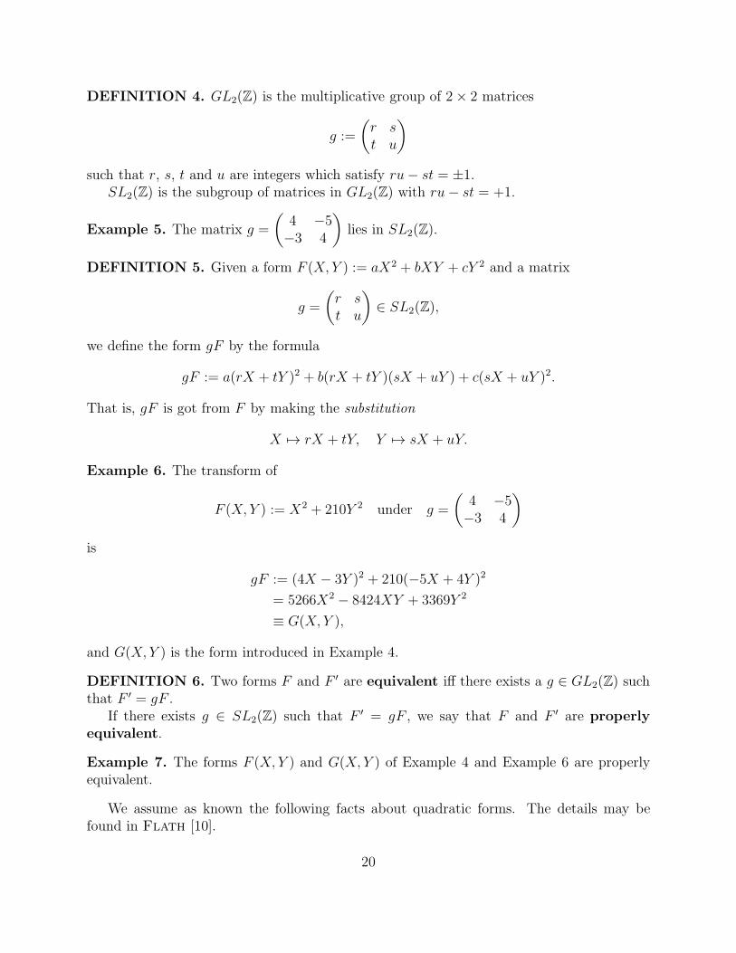
DEFINITION 4. GL2(Z) is the multiplicative group of 2× 2 matrices
g :=
(
r st u
)
such that r, s, t and u are integers which satisfy ru− st = ±1.SL2(Z) is the subgroup of matrices in GL2(Z) with ru− st = +1.
Example 5. The matrix g =
(
4 −5−3 4
)
lies in SL2(Z).
DEFINITION 5. Given a form F (X, Y ) := aX2 + bXY + cY 2 and a matrix
g =
(
r st u
)
∈ SL2(Z),
we define the form gF by the formula
gF := a(rX + tY )2 + b(rX + tY )(sX + uY ) + c(sX + uY )2.
That is, gF is got from F by making the substitution
X 7→ rX + tY, Y 7→ sX + uY.
Example 6. The transform of
F (X, Y ) := X2 + 210Y 2 under g =
(
4 −5−3 4
)
is
gF := (4X − 3Y )2 + 210(−5X + 4Y )2
= 5266X2 − 8424XY + 3369Y 2
≡ G(X, Y ),
and G(X, Y ) is the form introduced in Example 4.
DEFINITION 6. Two forms F and F ′ are equivalent iff there exists a g ∈ GL2(Z) suchthat F ′ = gF .
If there exists g ∈ SL2(Z) such that F ′ = gF , we say that F and F ′ are properlyequivalent.
Example 7. The forms F (X, Y ) and G(X, Y ) of Example 4 and Example 6 are properlyequivalent.
We assume as known the following facts about quadratic forms. The details may befound in Flath [10].
20
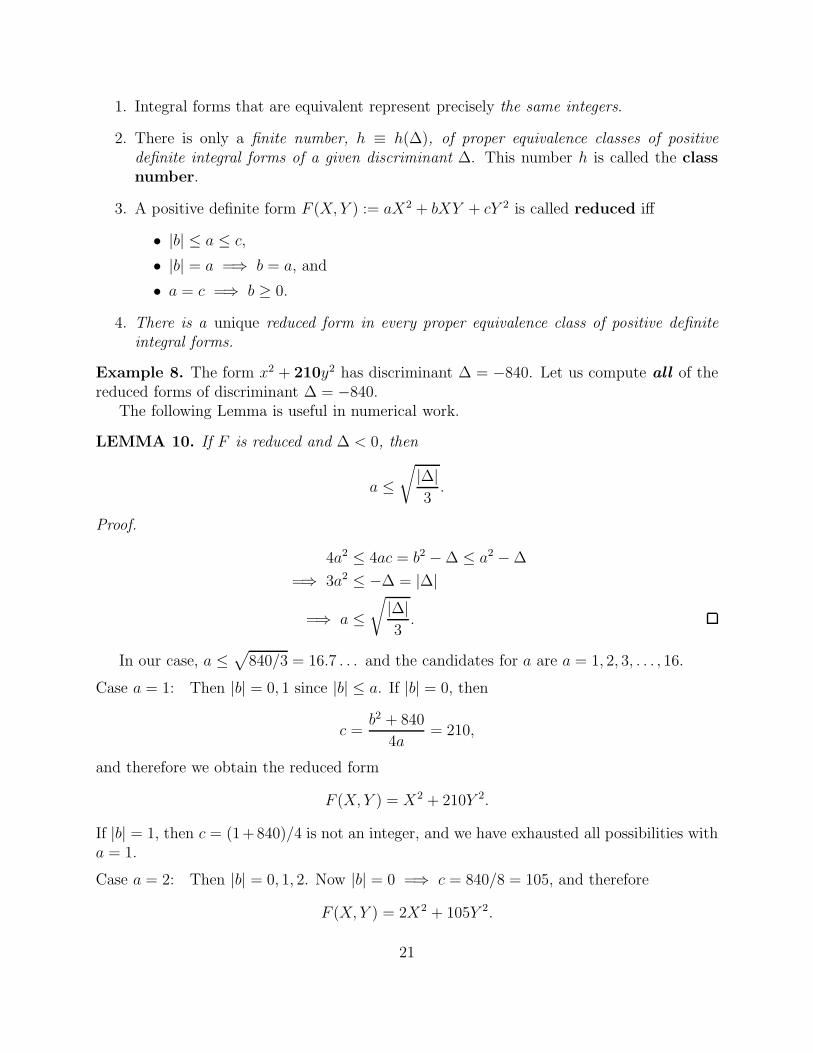
1. Integral forms that are equivalent represent precisely the same integers.
2. There is only a finite number, h ≡ h(∆), of proper equivalence classes of positive
definite integral forms of a given discriminant ∆. This number h is called the classnumber.
3. A positive definite form F (X, Y ) := aX2 + bXY + cY 2 is called reduced iff
• |b| ≤ a ≤ c,
• |b| = a =⇒ b = a, and
• a = c =⇒ b ≥ 0.
4. There is a unique reduced form in every proper equivalence class of positive definite
integral forms.
Example 8. The form x2 + 210y2 has discriminant ∆ = −840. Let us compute all of thereduced forms of discriminant ∆ = −840.
The following Lemma is useful in numerical work.
LEMMA 10. If F is reduced and ∆ < 0, then
a ≤√
|∆|3
.
Proof.
4a2 ≤ 4ac = b2 −∆ ≤ a2 −∆
=⇒ 3a2 ≤ −∆ = |∆|
=⇒ a ≤√
|∆|3
.
In our case, a ≤√
840/3 = 16.7 . . . and the candidates for a are a = 1, 2, 3, . . . , 16.
Case a = 1: Then |b| = 0, 1 since |b| ≤ a. If |b| = 0, then
c =b2 + 840
4a= 210,
and therefore we obtain the reduced form
F (X, Y ) = X2 + 210Y 2.
If |b| = 1, then c = (1+840)/4 is not an integer, and we have exhausted all possibilities witha = 1.
Case a = 2: Then |b| = 0, 1, 2. Now |b| = 0 =⇒ c = 840/8 = 105, and therefore
F (X, Y ) = 2X2 + 105Y 2.
21
On the other hand, |b| = 1 =⇒ c = 841/8, not an integer, and |b| = 2 =⇒ c = 844/8, notan integer either.
The remaining values of a are treated in the same way and we simply tabulate the finalresults.
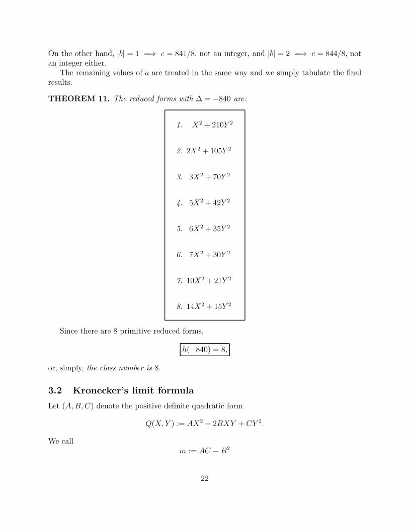
THEOREM 11. The reduced forms with ∆ = −840 are:
1. X2 + 210Y 2
2. 2X2 + 105Y 2
3. 3X2 + 70Y 2
4. 5X2 + 42Y 2
5. 6X2 + 35Y 2
6. 7X2 + 30Y 2
7. 10X2 + 21Y 2
8. 14X2 + 15Y 2
Since there are 8 primitive reduced forms,
h(−840) = 8,
or, simply, the class number is 8.
3.2 Kronecker’s limit formula
Let (A,B,C) denote the positive definite quadratic form
Q(X, Y ) := AX2 + 2BXY + CY 2.
We callm := AC −B2
22
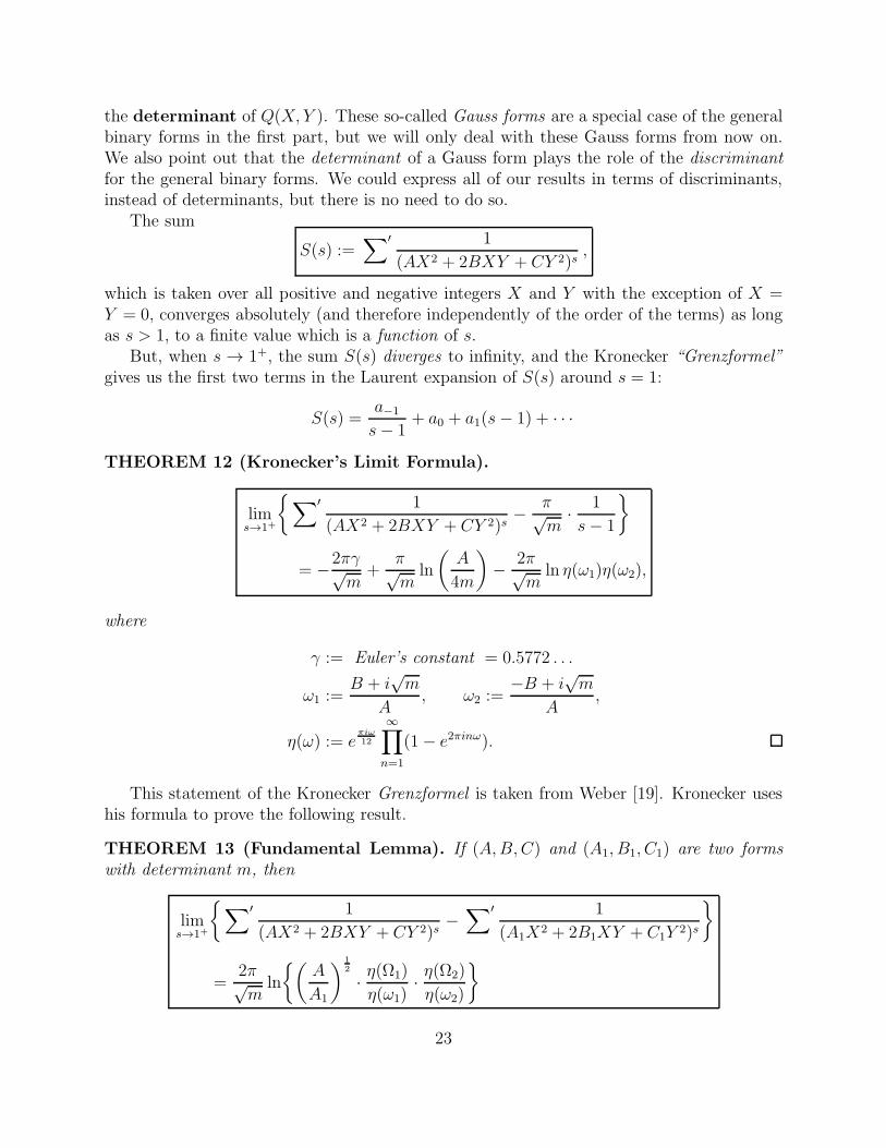
the determinant of Q(X, Y ). These so-called Gauss forms are a special case of the generalbinary forms in the first part, but we will only deal with these Gauss forms from now on.We also point out that the determinant of a Gauss form plays the role of the discriminant
for the general binary forms. We could express all of our results in terms of discriminants,instead of determinants, but there is no need to do so.
The sum
S(s) :=∑′ 1
(AX2 + 2BXY + CY 2)s,
which is taken over all positive and negative integers X and Y with the exception of X =Y = 0, converges absolutely (and therefore independently of the order of the terms) as longas s > 1, to a finite value which is a function of s.
But, when s → 1+, the sum S(s) diverges to infinity, and the Kronecker “Grenzformel”
gives us the first two terms in the Laurent expansion of S(s) around s = 1:
S(s) =a−1
s− 1+ a0 + a1(s− 1) + · · ·
THEOREM 12 (Kronecker’s Limit Formula).
lims→1+
∑′ 1
(AX2 + 2BXY + CY 2)s− π√
m· 1
s− 1
= −2πγ√m
+π√m
ln
(
A
4m
)
− 2π√m
ln η(ω1)η(ω2),
where
γ := Euler’s constant = 0.5772 . . .
ω1 :=B + i
√m
A, ω2 :=
−B + i√m
A,
η(ω) := eπiω
12
∞∏
n=1
(1− e2πinω).
This statement of the Kronecker Grenzformel is taken from Weber [19]. Kronecker useshis formula to prove the following result.
THEOREM 13 (Fundamental Lemma). If (A,B,C) and (A1, B1, C1) are two forms
with determinant m, then
lims→1+
∑′ 1
(AX2 + 2BXY + CY 2)s−∑′ 1
(A1X2 + 2B1XY + C1Y 2)s
=2π√m
ln
(
A
A1
) 1
2
· η(Ω1)
η(ω1)· η(Ω2)
η(ω2)
23
where
ω1 :=B + i
√m
A, ω2 :=
−B + i√m
A,
Ω1 :=B1 + i
√m
A1, Ω2 :=
−B1 + i√m
A1.
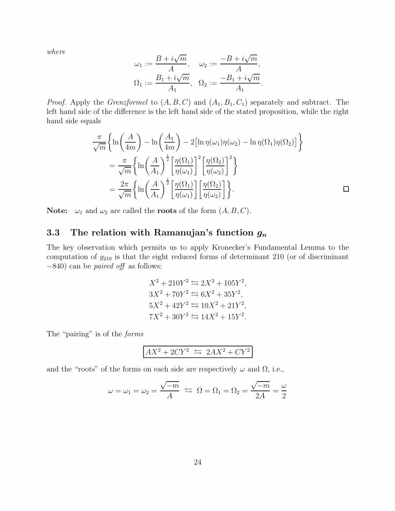
Proof. Apply the Grenzformel to (A,B,C) and (A1, B1, C1) separately and subtract. Theleft hand side of the difference is the left hand side of the stated proposition, while the righthand side equals
π√m
ln
(
A
4m
)
− ln
(
A1
4m
)
− 2[
ln η(ω1)η(ω2)− ln η(Ω1)η(Ω2)]
=π√m
ln
(
A
A1
) 1
2[
η(Ω1)
η(ω1)
]2[η(Ω2)
η(ω2)
]2
=2π√m
ln
(
A
A1
)1
2[
η(Ω1)
η(ω1)
][
η(Ω2)
η(ω2)
]
.
Note: ω1 and ω2 are called the roots of the form (A,B,C).
3.3 The relation with Ramanujan’s function gn
The key observation which permits us to apply Kronecker’s Fundamental Lemma to thecomputation of g210 is that the eight reduced forms of determinant 210 (or of discriminant−840) can be paired off as follows:
X2 + 210Y 2 2X2 + 105Y 2,
3X2 + 70Y 2 6X2 + 35Y 2,
5X2 + 42Y 2 10X2 + 21Y 2,
7X2 + 30Y 2 14X2 + 15Y 2.
The “pairing” is of the forms
AX2 + 2CY 2 2AX2 + CY 2
and the “roots” of the forms on each side are respectively ω and Ω, i.e.,
ω = ω1 = ω2 =
√−m
A Ω = Ω1 = Ω2 =
√−m
2A=
ω
2
24
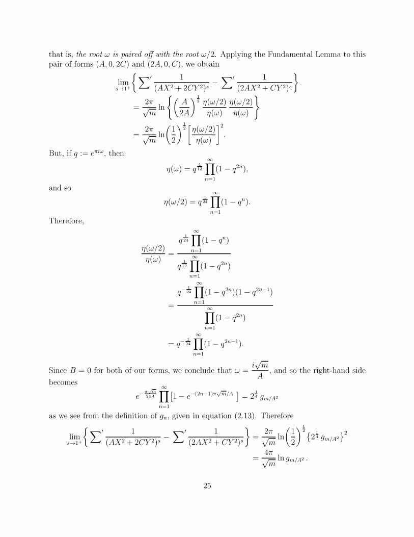
that is, the root ω is paired off with the root ω/2. Applying the Fundamental Lemma to thispair of forms (A, 0, 2C) and (2A, 0, C), we obtain
lims→1+
∑′ 1
(AX2 + 2CY 2)s−∑′ 1
(2AX2 + CY 2)s
=2π√m
ln
(
A
2A
)1
2 η(ω/2)
η(ω)
η(ω/2)
η(ω)
=2π√m
ln
(
1
2
)1
2[
η(ω/2)
η(ω)
]2
.
But, if q := eπiω, then
η(ω) = q1
12
∞∏
n=1
(1− q2n),
and so
η(ω/2) = q1
24
∞∏
n=1
(1− qn).
Therefore,
η(ω/2)
η(ω)=
q1
24
∞∏
n=1
(1− qn)
q1
12
∞∏
n=1
(1− q2n)
=
q−1
24
∞∏
n=1
(1− q2n)(1− q2n−1)
∞∏
n=1
(1− q2n)
= q−1
24
∞∏
n=1
(1− q2n−1).
Since B = 0 for both of our forms, we conclude that ω =i√m
A, and so the right-hand side
becomes
e−π√
m
24A
∞∏
n=1
[
1− e−(2n−1)π√m/A
]
= 21
4 gm/A2
as we see from the definition of gn, given in equation (2.13). Therefore
lims→1+
∑′ 1
(AX2 + 2CY 2)s−∑′ 1
(2AX2 + CY 2)s
=2π√m
ln
(
1
2
) 1
2
21
4 gm/A2
2
=4π√m
ln gm/A2 .
25
We have therefore obtained the following formula.
THEOREM 14 (Kronecker’s Formula for gn).
lims→1+
∑′ 1
(AX2 + 2CY 2)s−∑′ 1
(2AX2 + CY 2)s
=4π√m
ln gm/A2 . (G)
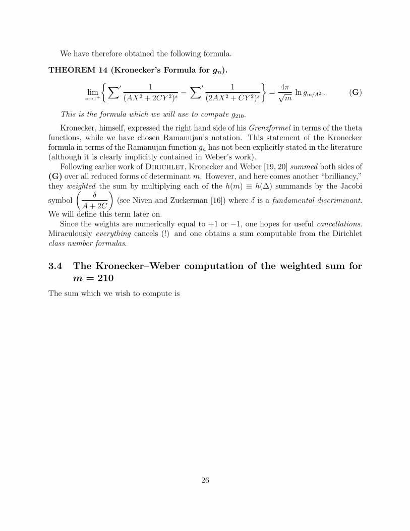
This is the formula which we will use to compute g210.
Kronecker, himself, expressed the right hand side of his Grenzformel in terms of the thetafunctions, while we have chosen Ramanujan’s notation. This statement of the Kroneckerformula in terms of the Ramanujan function gn has not been explicitly stated in the literature(although it is clearly implicitly contained in Weber’s work).
Following earlier work of Dirichlet, Kronecker and Weber [19, 20] summed both sides of(G) over all reduced forms of determinant m. However, and here comes another “brilliancy,”they weighted the sum by multiplying each of the h(m) ≡ h(∆) summands by the Jacobi
symbol
(
δ
A+ 2C
)
(see Niven and Zuckerman [16]) where δ is a fundamental discriminant.
We will define this term later on.Since the weights are numerically equal to +1 or −1, one hopes for useful cancellations.
Miraculously everything cancels (!) and one obtains a sum computable from the Dirichletclass number formulas.
3.4 The Kronecker–Weber computation of the weighted sum for
m = 210
The sum which we wish to compute is
26
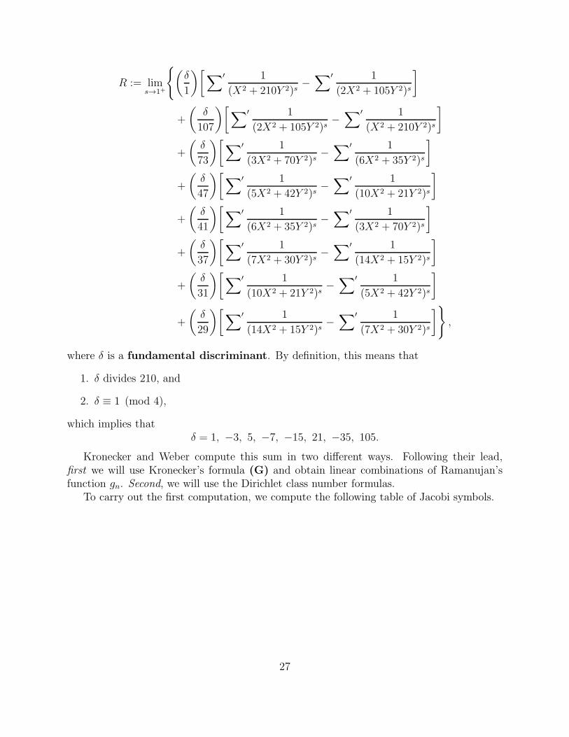
R := lims→1+
(
δ
1
)[
∑′ 1
(X2 + 210Y 2)s−∑′ 1
(2X2 + 105Y 2)s
]
+
(
δ
107
)[
∑′ 1
(2X2 + 105Y 2)s−∑′ 1
(X2 + 210Y 2)s
]
+
(
δ
73
)[
∑′ 1
(3X2 + 70Y 2)s−∑′ 1
(6X2 + 35Y 2)s
]
+
(
δ
47
)[
∑′ 1
(5X2 + 42Y 2)s−∑′ 1
(10X2 + 21Y 2)s
]
+
(
δ
41
)[
∑′ 1
(6X2 + 35Y 2)s−∑′ 1
(3X2 + 70Y 2)s
]
+
(
δ
37
)[
∑′ 1
(7X2 + 30Y 2)s−∑′ 1
(14X2 + 15Y 2)s
]
+
(
δ
31
)[
∑′ 1
(10X2 + 21Y 2)s−∑′ 1
(5X2 + 42Y 2)s
]
+
(
δ
29
)[
∑′ 1
(14X2 + 15Y 2)s−∑′ 1
(7X2 + 30Y 2)s
]
,
where δ is a fundamental discriminant. By definition, this means that
1. δ divides 210, and
2. δ ≡ 1 (mod 4),
which implies thatδ = 1, −3, 5, −7, −15, 21, −35, 105.
Kronecker and Weber compute this sum in two different ways. Following their lead,first we will use Kronecker’s formula (G) and obtain linear combinations of Ramanujan’sfunction gn. Second, we will use the Dirichlet class number formulas.
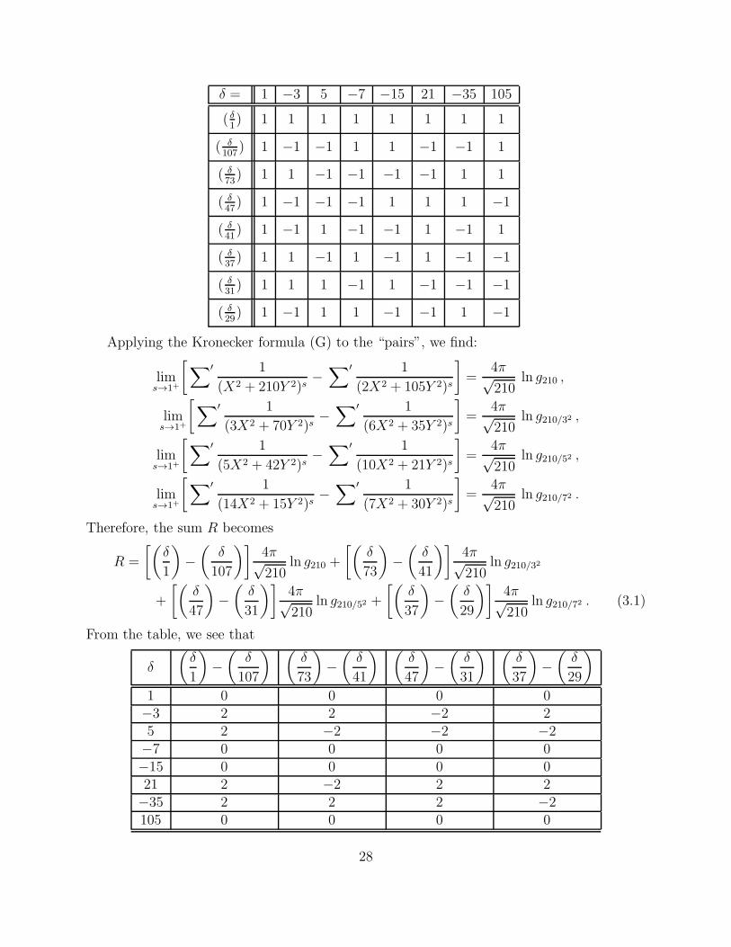
To carry out the first computation, we compute the following table of Jacobi symbols.
27
δ = 1 −3 5 −7 −15 21 −35 105
( δ1) 1 1 1 1 1 1 1 1
( δ107
) 1 −1 −1 1 1 −1 −1 1
( δ73) 1 1 −1 −1 −1 −1 1 1
( δ47) 1 −1 −1 −1 1 1 1 −1
( δ41) 1 −1 1 −1 −1 1 −1 1
( δ37) 1 1 −1 1 −1 1 −1 −1
( δ31) 1 1 1 −1 1 −1 −1 −1
( δ29) 1 −1 1 1 −1 −1 1 −1
Applying the Kronecker formula (G) to the “pairs”, we find:
lims→1+
[
∑′ 1
(X2 + 210Y 2)s−∑′ 1
(2X2 + 105Y 2)s
]
=4π√210
ln g210 ,
lims→1+
[
∑′ 1
(3X2 + 70Y 2)s−∑′ 1
(6X2 + 35Y 2)s
]
=4π√210
ln g210/32 ,
lims→1+
[
∑′ 1
(5X2 + 42Y 2)s−∑′ 1
(10X2 + 21Y 2)s
]
=4π√210
ln g210/52 ,
lims→1+
[
∑′ 1
(14X2 + 15Y 2)s−∑′ 1
(7X2 + 30Y 2)s
]
=4π√210
ln g210/72 .
Therefore, the sum R becomes
R =
[(
δ
1
)
−(
δ
107
)]
4π√210
ln g210 +
[(
δ
73
)
−(
δ
41
)]
4π√210
ln g210/32
+
[(
δ
47
)
−(
δ
31
)]
4π√210
ln g210/52 +
[(
δ
37
)
−(
δ
29
)]
4π√210
ln g210/72 . (3.1)
From the table, we see that
δ
(
δ
1
)
−(
δ
107
) (
δ
73
)
−(
δ
41
) (
δ
47
)
−(
δ
31
) (
δ
37
)
−(
δ
29
)
1 0 0 0 0−3 2 2 −2 25 2 −2 −2 −2−7 0 0 0 0−15 0 0 0 021 2 −2 2 2−35 2 2 2 −2105 0 0 0 0
28
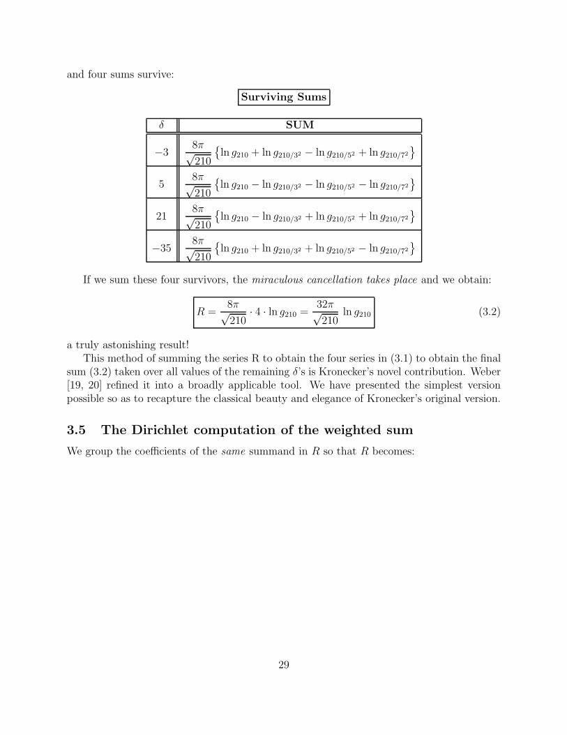
and four sums survive:
Surviving Sums
δ SUM
−38π√210
ln g210 + ln g210/32 − ln g210/52 + ln g210/72
58π√210
ln g210 − ln g210/32 − ln g210/52 − ln g210/72
218π√210
ln g210 − ln g210/32 + ln g210/52 + ln g210/72
−358π√210
ln g210 + ln g210/32 + ln g210/52 − ln g210/72
If we sum these four survivors, the miraculous cancellation takes place and we obtain:
R =8π√210
· 4 · ln g210 =32π√210
ln g210 (3.2)
a truly astonishing result!This method of summing the series R to obtain the four series in (3.1) to obtain the final
sum (3.2) taken over all values of the remaining δ’s is Kronecker’s novel contribution. Weber[19, 20] refined it into a broadly applicable tool. We have presented the simplest versionpossible so as to recapture the classical beauty and elegance of Kronecker’s original version.
3.5 The Dirichlet computation of the weighted sum
We group the coefficients of the same summand in R so that R becomes:
29
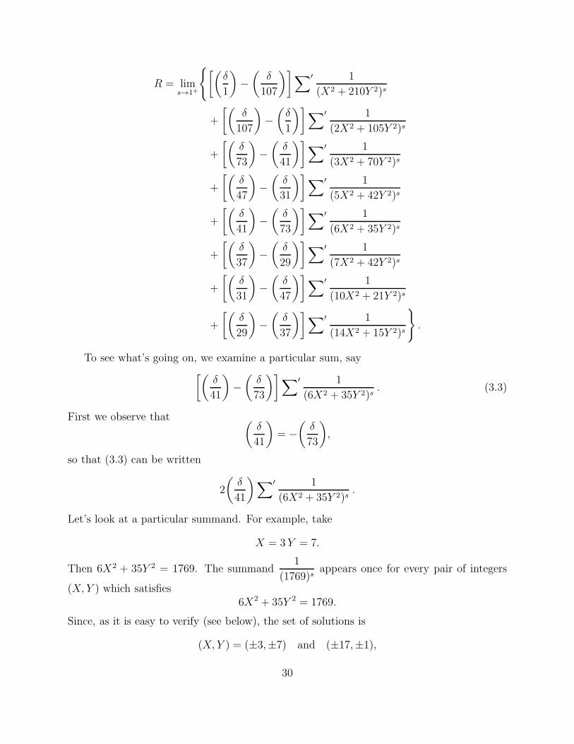
R = lims→1+
[(
δ
1
)
−(
δ
107
)]
∑′ 1
(X2 + 210Y 2)s
+
[(
δ
107
)
−(
δ
1
)]
∑′ 1
(2X2 + 105Y 2)s
+
[(
δ
73
)
−(
δ
41
)]
∑′ 1
(3X2 + 70Y 2)s
+
[(
δ
47
)
−(
δ
31
)]
∑′ 1
(5X2 + 42Y 2)s
+
[(
δ
41
)
−(
δ
73
)]
∑′ 1
(6X2 + 35Y 2)s
+
[(
δ
37
)
−(
δ
29
)]
∑′ 1
(7X2 + 42Y 2)s
+
[(
δ
31
)
−(
δ
47
)]
∑′ 1
(10X2 + 21Y 2)s
+
[(
δ
29
)
−(
δ
37
)]
∑′ 1
(14X2 + 15Y 2)s
.
To see what’s going on, we examine a particular sum, say[(
δ
41
)
−(
δ
73
)]
∑′ 1
(6X2 + 35Y 2)s. (3.3)
First we observe that(
δ
41
)
= −(
δ
73
)
,
so that (3.3) can be written
2
(
δ
41
)
∑′ 1
(6X2 + 35Y 2)s.
Let’s look at a particular summand. For example, take
X = 3 Y = 7.
Then 6X2 + 35Y 2 = 1769. The summand1
(1769)sappears once for every pair of integers
(X, Y ) which satisfies6X2 + 35Y 2 = 1769.
Since, as it is easy to verify (see below), the set of solutions is
(X, Y ) = (±3,±7) and (±17,±1),
30
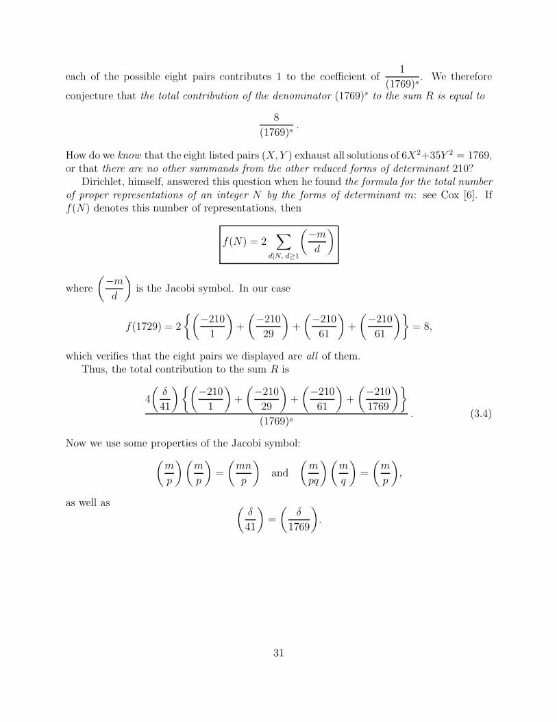
each of the possible eight pairs contributes 1 to the coefficient of1
(1769)s. We therefore
conjecture that the total contribution of the denominator (1769)s to the sum R is equal to
8
(1769)s.
How do we know that the eight listed pairs (X, Y ) exhaust all solutions of 6X2+35Y 2 = 1769,or that there are no other summands from the other reduced forms of determinant 210?
Dirichlet, himself, answered this question when he found the formula for the total number
of proper representations of an integer N by the forms of determinant m: see Cox [6]. Iff(N) denotes this number of representations, then
f(N) = 2∑
d|N, d≥1
(−m
d
)
where
(−m
d
)
is the Jacobi symbol. In our case
f(1729) = 2
(−210
1
)
+
(−210
29
)
+
(−210
61
)
+
(−210
61
)
= 8,
which verifies that the eight pairs we displayed are all of them.Thus, the total contribution to the sum R is
4
(
δ
41
)(−210
1
)
+
(−210
29
)
+
(−210
61
)
+
(−210
1769
)
(1769)s. (3.4)
Now we use some properties of the Jacobi symbol:
(
m
p
)(
m
p
)
=
(
mn
p
)
and
(
m
pq
)(
m
q
)
=
(
m
p
)
,
as well as(
δ
41
)
=
(
δ
1769
)
.
31
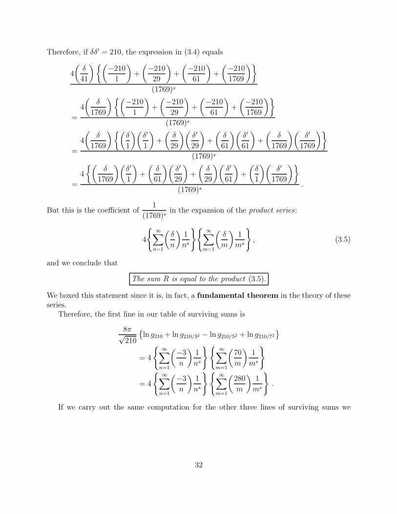
Therefore, if δδ′ = 210, the expression in (3.4) equals
4
(
δ
41
)(−210
1
)
+
(−210
29
)
+
(−210
61
)
+
(−210
1769
)
(1769)s
=
4
(
δ
1769
)(−210
1
)
+
(−210
29
)
+
(−210
61
)
+
(−210
1769
)
(1769)s
=
4
(
δ
1769
)(
δ
1
)(
δ′
1
)
+
(
δ
29
)(
δ′
29
)
+
(
δ
61
)(
δ′
61
)
+
(
δ
1769
)(
δ′
1769
)
(1769)s
=
4
(
δ
1769
)(
δ′
1
)
+
(
δ
61
)(
δ′
29
)
+
(
δ
29
)(
δ′
61
)
+
(
δ
1
)(
δ′
1769
)
(1769)s.
But this is the coefficient of1
(1769)sin the expansion of the product series :
4
∞∑
n=1
(
δ
n
)
1
ns
∞∑
m=1
(
δ
m
)
1
ms
, (3.5)
and we conclude that
The sum R is equal to the product (3.5).
We boxed this statement since it is, in fact, a fundamental theorem in the theory of theseseries.
Therefore, the first line in our table of surviving sums is
8π√210
ln g210 + ln g210/32 − ln g210/52 + ln g210/72
= 4
∞∑
n=1
(−3
n
)
1
ns
∞∑
m=1
(
70
m
)
1
ms
= 4
∞∑
n=1
(−3
n
)
1
ns
∞∑
m=1
(
280
m
)
1
ms
.
If we carry out the same computation for the other three lines of surviving sums we
32
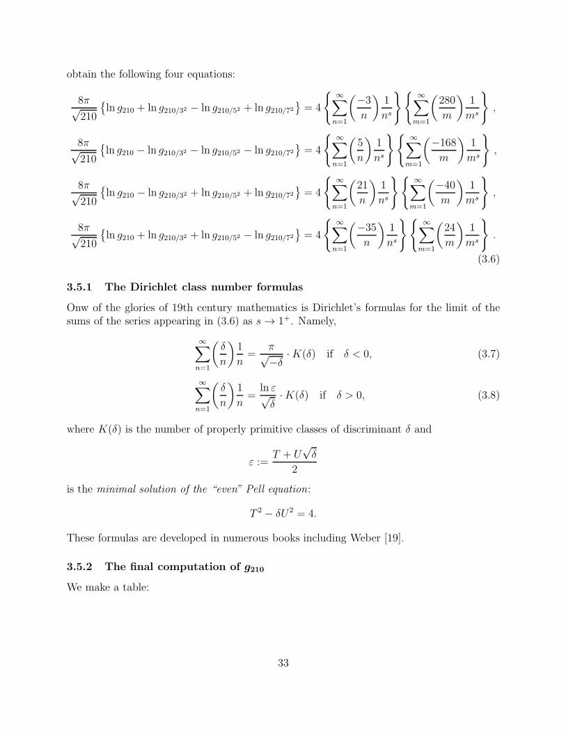
obtain the following four equations:
8π√210
ln g210 + ln g210/32 − ln g210/52 + ln g210/72
= 4
∞∑
n=1
(−3
n
)
1
ns
∞∑
m=1
(
280
m
)
1
ms
,
8π√210
ln g210 − ln g210/32 − ln g210/52 − ln g210/72
= 4
∞∑
n=1
(
5
n
)
1
ns
∞∑
m=1
(−168
m
)
1
ms
,
8π√210
ln g210 − ln g210/32 + ln g210/52 + ln g210/72
= 4
∞∑
n=1
(
21
n
)
1
ns
∞∑
m=1
(−40
m
)
1
ms
,
8π√210
ln g210 + ln g210/32 + ln g210/52 − ln g210/72
= 4
∞∑
n=1
(−35
n
)
1
ns
∞∑
m=1
(
24
m
)
1
ms
.
(3.6)
3.5.1 The Dirichlet class number formulas
Onw of the glories of 19th century mathematics is Dirichlet’s formulas for the limit of thesums of the series appearing in (3.6) as s → 1+. Namely,
∞∑
n=1
(
δ
n
)
1
n=
π√−δ
·K(δ) if δ < 0, (3.7)
∞∑
n=1
(
δ
n
)
1
n=
ln ε√δ·K(δ) if δ > 0, (3.8)
where K(δ) is the number of properly primitive classes of discriminant δ and
ε :=T + U
√δ
2
is the minimal solution of the “even” Pell equation:
T 2 − δU2 = 4.
These formulas are developed in numerous books including Weber [19].
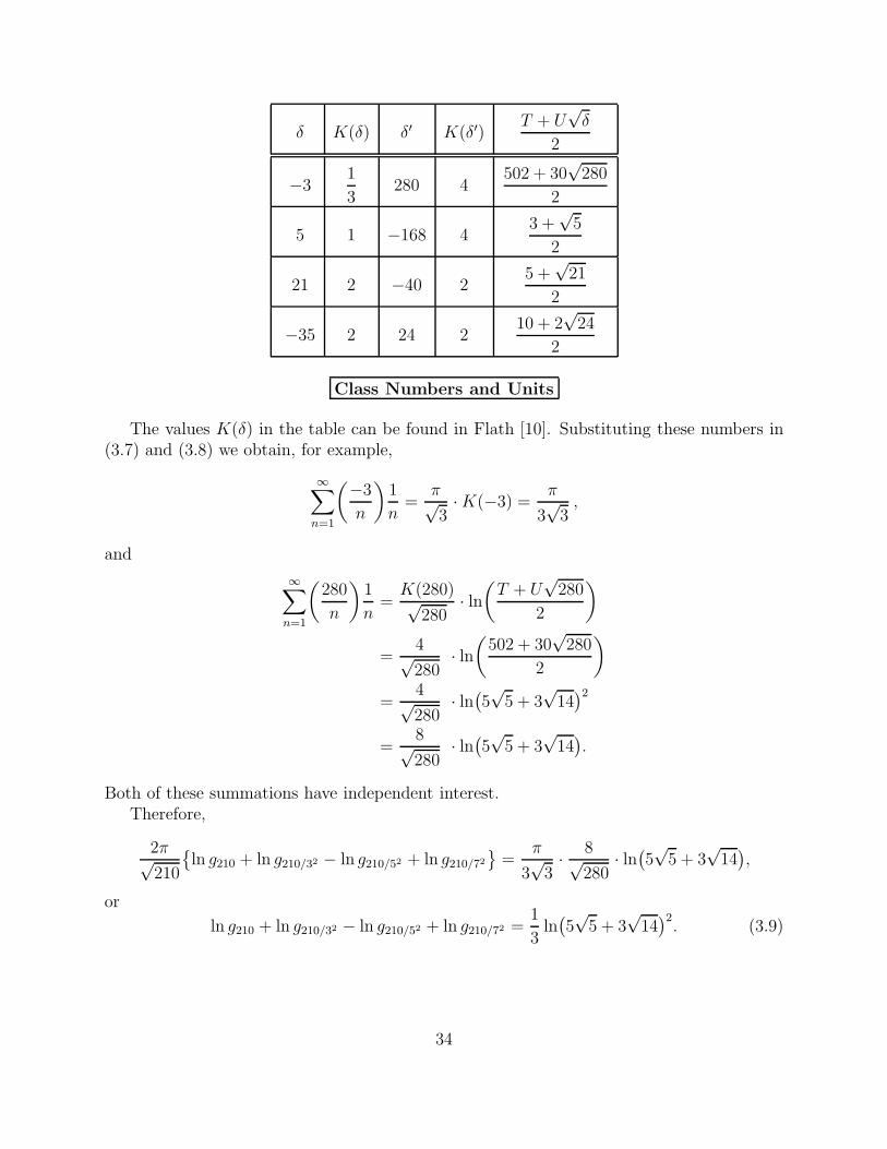
3.5.2 The final computation of g210
We make a table:
33
δ K(δ) δ′ K(δ′)T + U
√δ
2
−31
3280 4
502 + 30√280
2
5 1 −168 43 +
√5
2
21 2 −40 25 +
√21
2
−35 2 24 210 + 2
√24
2
Class Numbers and Units
The values K(δ) in the table can be found in Flath [10]. Substituting these numbers in(3.7) and (3.8) we obtain, for example,
∞∑
n=1
(−3
n
)
1
n=
π√3·K(−3) =
π
3√3,
and
∞∑
n=1
(
280
n
)
1
n=
K(280)√280
· ln(
T + U√280
2
)
=4√280
· ln(
502 + 30√280
2
)
=4√280
· ln(
5√5 + 3
√14)2
=8√280
· ln(
5√5 + 3
√14)
.
Both of these summations have independent interest.Therefore,
2π√210
ln g210 + ln g210/32 − ln g210/52 + ln g210/72
=π
3√3· 8√
280· ln(
5√5 + 3
√14)
,
or
ln g210 + ln g210/32 − ln g210/52 + ln g210/72 =1
3ln(
5√5 + 3
√14)2. (3.9)
34
The Dirichlet class number formulas applied the three remaining product series give us
4
∞∑
n=1
(
5
n
)
1
ns
∞∑
m=1
(−168
m
)
1
ms
=π√210
1 · 42
ln
(
3 +√5
2
)
· 4,
4
∞∑
n=1
(
21
n
)
1
ns
∞∑
m=1
(−40
m
)
1
ms
=π√210
2 · 22
ln
(
5 +√21
2
)
· 4,
4
∞∑
n=1
(−35
n
)
1
ns
∞∑
m=1
(
24
m
)
1
ms
=π√210
2 · 22
ln
(
10 + 2√24
2
)
· 4.
Thus the last three lines of (3.6) permit us to conclude
ln g210 − ln g210/32 − ln g210/52 − ln g210/72 = ln
(
3 +√5
2
)
,
ln g210 − ln g210/32 + ln g210/52 + ln g210/72 = ln
(
5 +√21
2
)
,
ln g210 + ln g210/32 + ln g210/52 − ln g210/72 = ln
(
10 + 2√24
2
)
. (3.10)
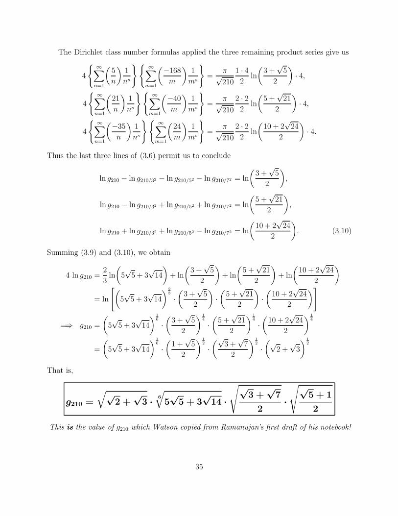
Summing (3.9) and (3.10), we obtain
4 ln g210 =2
3ln
(
5√5 + 3
√14
)
+ ln
(
3 +√5
2
)
+ ln
(
5 +√21
2
)
+ ln
(
10 + 2√24
2
)
= ln
[
(
5√5 + 3
√14
)2
3
·(
3 +√5
2
)
·(
5 +√21
2
)
·(
10 + 2√24
2
)
]
=⇒ g210 =
(
5√5 + 3
√14
)1
6
·(
3 +√5
2
)1
4
·(
5 +√21
2
)1
4
·(
10 + 2√24
2
)1
4
=
(
5√5 + 3
√14
)1
6
·(
1 +√5
2
)1
2
·(√3 +
√7
2
)1
2
·(√
2 +√3
)1
2
That is,
g210 =
√
√
2 +√
3 ·6
√
5√
5 + 3√
14 ·
√
√3 +
√7
2·
√
√5 + 1
2
This is the value of g210 which Watson copied from Ramanujan’s first draft of his notebook!
35
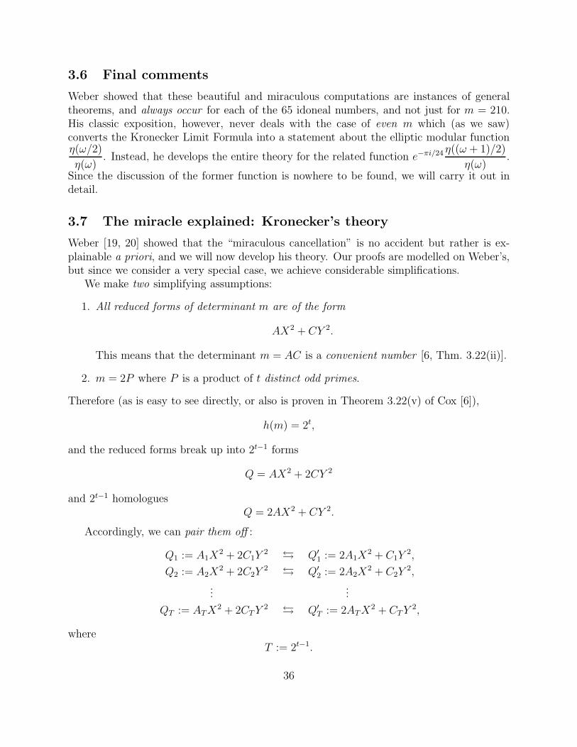
3.6 Final comments
Weber showed that these beautiful and miraculous computations are instances of generaltheorems, and always occur for each of the 65 idoneal numbers, and not just for m = 210.His classic exposition, however, never deals with the case of even m which (as we saw)converts the Kronecker Limit Formula into a statement about the elliptic modular functionη(ω/2)
η(ω). Instead, he develops the entire theory for the related function e−πi/24 η((ω + 1)/2)
η(ω).
Since the discussion of the former function is nowhere to be found, we will carry it out indetail.
3.7 The miracle explained: Kronecker’s theory
Weber [19, 20] showed that the “miraculous cancellation” is no accident but rather is ex-plainable a priori, and we will now develop his theory. Our proofs are modelled on Weber’s,but since we consider a very special case, we achieve considerable simplifications.
We make two simplifying assumptions:
1. All reduced forms of determinant m are of the form
AX2 + CY 2.
This means that the determinant m = AC is a convenient number [6, Thm. 3.22(ii)].
2. m = 2P where P is a product of t distinct odd primes.
Therefore (as is easy to see directly, or also is proven in Theorem 3.22(v) of Cox [6]),
h(m) = 2t,
and the reduced forms break up into 2t−1 forms
Q = AX2 + 2CY 2
and 2t−1 homologuesQ = 2AX2 + CY 2.
Accordingly, we can pair them off :
Q1 := A1X2 + 2C1Y
2 Q′
1 := 2A1X2 + C1Y
2,
Q2 := A2X2 + 2C2Y
2 Q′
2 := 2A2X2 + C2Y
2,
......
QT := ATX2 + 2CTY
2 Q′
T := 2ATX2 + CTY
2,
whereT := 2t−1.
36
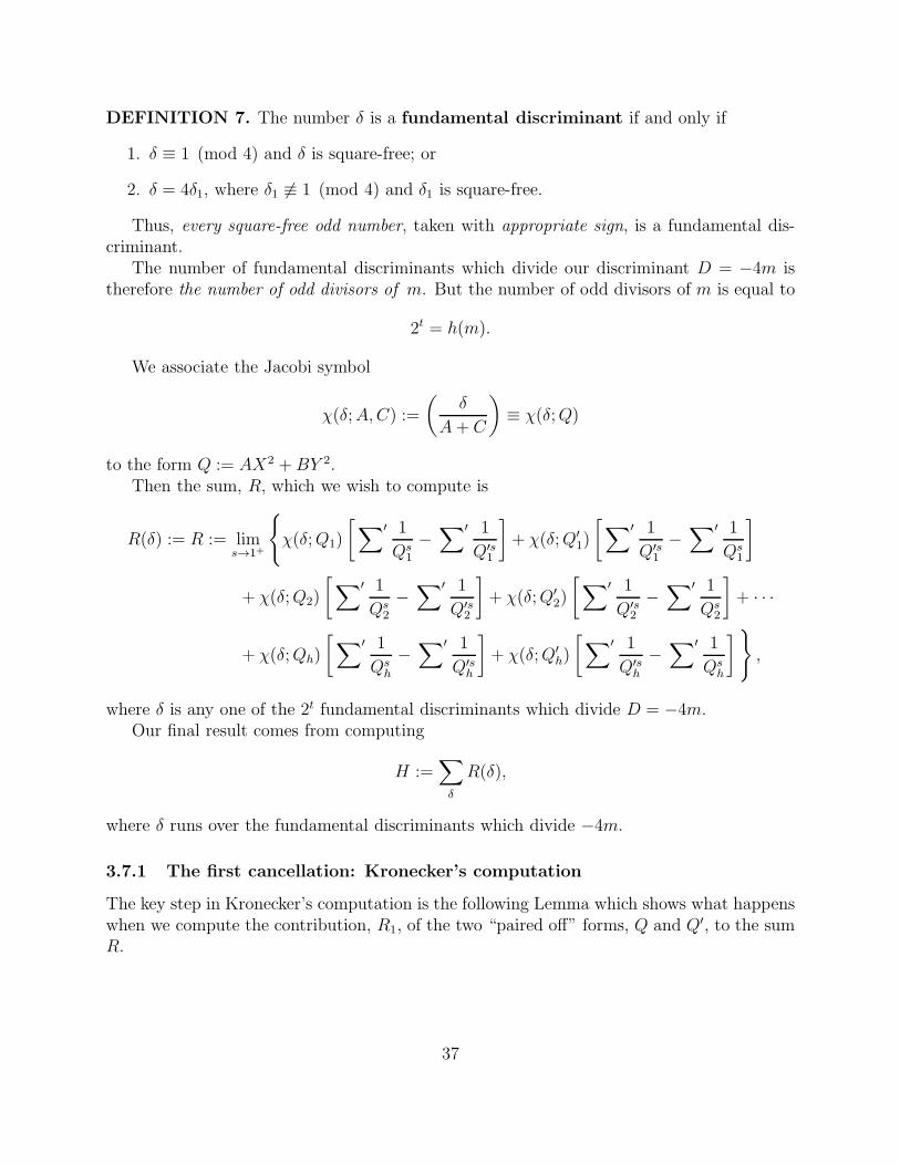
DEFINITION 7. The number δ is a fundamental discriminant if and only if
1. δ ≡ 1 (mod 4) and δ is square-free; or
2. δ = 4δ1, where δ1 6≡ 1 (mod 4) and δ1 is square-free.
Thus, every square-free odd number, taken with appropriate sign, is a fundamental dis-criminant.
The number of fundamental discriminants which divide our discriminant D = −4m istherefore the number of odd divisors of m. But the number of odd divisors of m is equal to
2t = h(m).
We associate the Jacobi symbol
χ(δ;A,C) :=
(
δ
A+ C
)
≡ χ(δ;Q)
to the form Q := AX2 +BY 2.Then the sum, R, which we wish to compute is
R(δ) := R := lims→1+
χ(δ;Q1)
[
∑′ 1
Qs1
−∑′ 1
Q′s1
]
+ χ(δ;Q′1)
[
∑′ 1
Q′s1
−∑′ 1
Qs1
]
+ χ(δ;Q2)
[
∑′ 1
Qs2
−∑′ 1
Q′s2
]
+ χ(δ;Q′2)
[
∑′ 1
Q′s2
−∑′ 1
Qs2
]
+ · · ·
+ χ(δ;Qh)
[
∑′ 1
Qsh
−∑′ 1
Q′sh
]
+ χ(δ;Q′h)
[
∑′ 1
Q′sh
−∑′ 1
Qsh
]
,
where δ is any one of the 2t fundamental discriminants which divide D = −4m.Our final result comes from computing
H :=∑
δ
R(δ),
where δ runs over the fundamental discriminants which divide −4m.
3.7.1 The first cancellation: Kronecker’s computation
The key step in Kronecker’s computation is the following Lemma which shows what happenswhen we compute the contribution, R1, of the two “paired off” forms, Q and Q′, to the sumR.
37
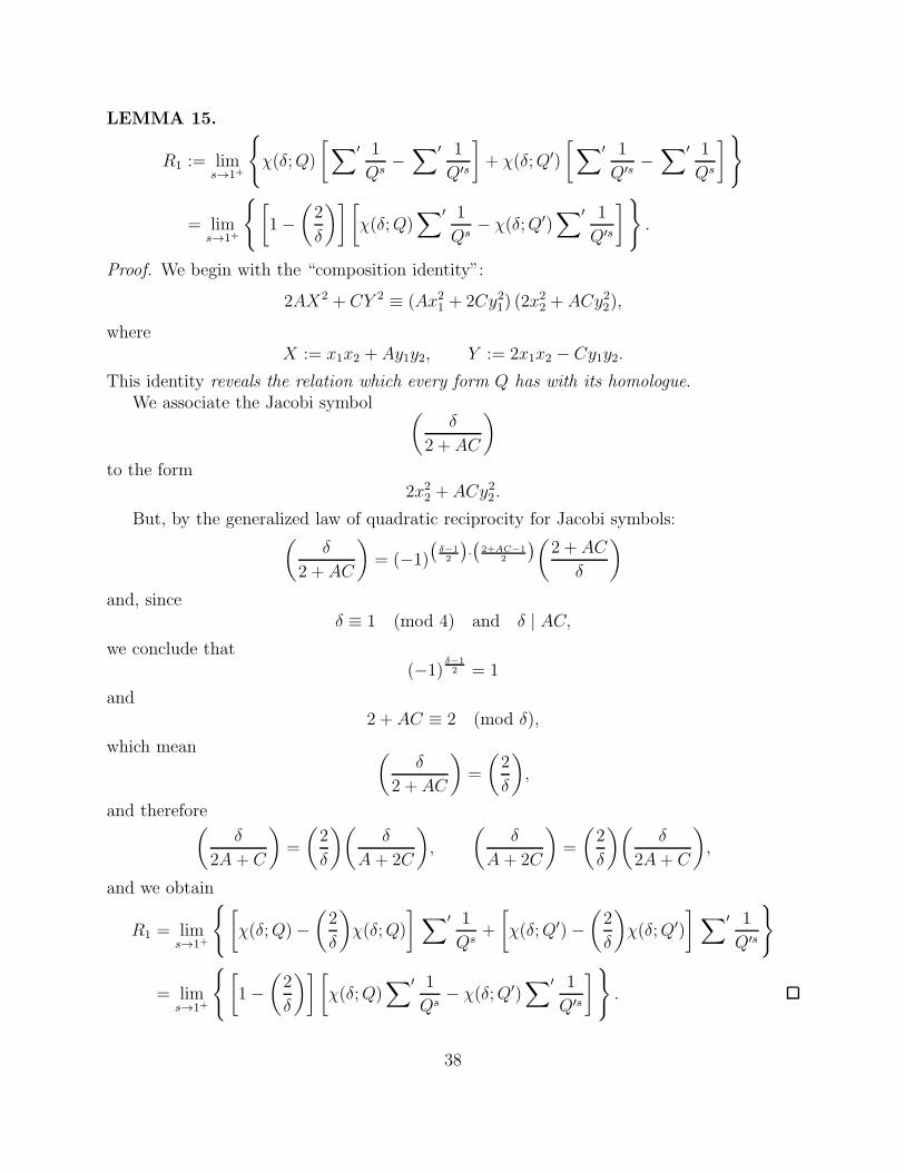
LEMMA 15.
R1 := lims→1+
χ(δ;Q)
[
∑′ 1
Qs−∑′ 1
Q′s
]
+ χ(δ;Q′)
[
∑′ 1
Q′s −∑′ 1
Qs
]
= lims→1+
[
1−(
2
δ
)][
χ(δ;Q)∑′ 1
Qs− χ(δ;Q′)
∑′ 1
Q′s
]
.
Proof. We begin with the “composition identity”:
2AX2 + CY 2 ≡ (Ax21 + 2Cy21) (2x
22 + ACy22),
whereX := x1x2 + Ay1y2, Y := 2x1x2 − Cy1y2.
This identity reveals the relation which every form Q has with its homologue.We associate the Jacobi symbol
(
δ
2 + AC
)
to the form2x2
2 + ACy22.
But, by the generalized law of quadratic reciprocity for Jacobi symbols:(
δ
2 + AC
)
= (−1)
(
δ−1
2
)
·(
2+AC−1
2
)
(
2 + AC
δ
)
and, sinceδ ≡ 1 (mod 4) and δ | AC,
we conclude that(−1)
δ−1
2 = 1
and2 + AC ≡ 2 (mod δ),
which mean(
δ
2 + AC
)
=
(
2
δ
)
,
and therefore(
δ
2A+ C
)
=
(
2
δ
)(
δ
A+ 2C
)
,
(
δ
A+ 2C
)
=
(
2
δ
)(
δ
2A+ C
)
,
and we obtain
R1 = lims→1+
[
χ(δ;Q)−(
2
δ
)
χ(δ;Q)
]
∑′ 1
Qs+
[
χ(δ;Q′)−(
2
δ
)
χ(δ;Q′)
]
∑′ 1
Q′s
= lims→1+
[
1−(
2
δ
)][
χ(δ;Q)∑′ 1
Qs− χ(δ;Q′)
∑′ 1
Q′s
]
.
38
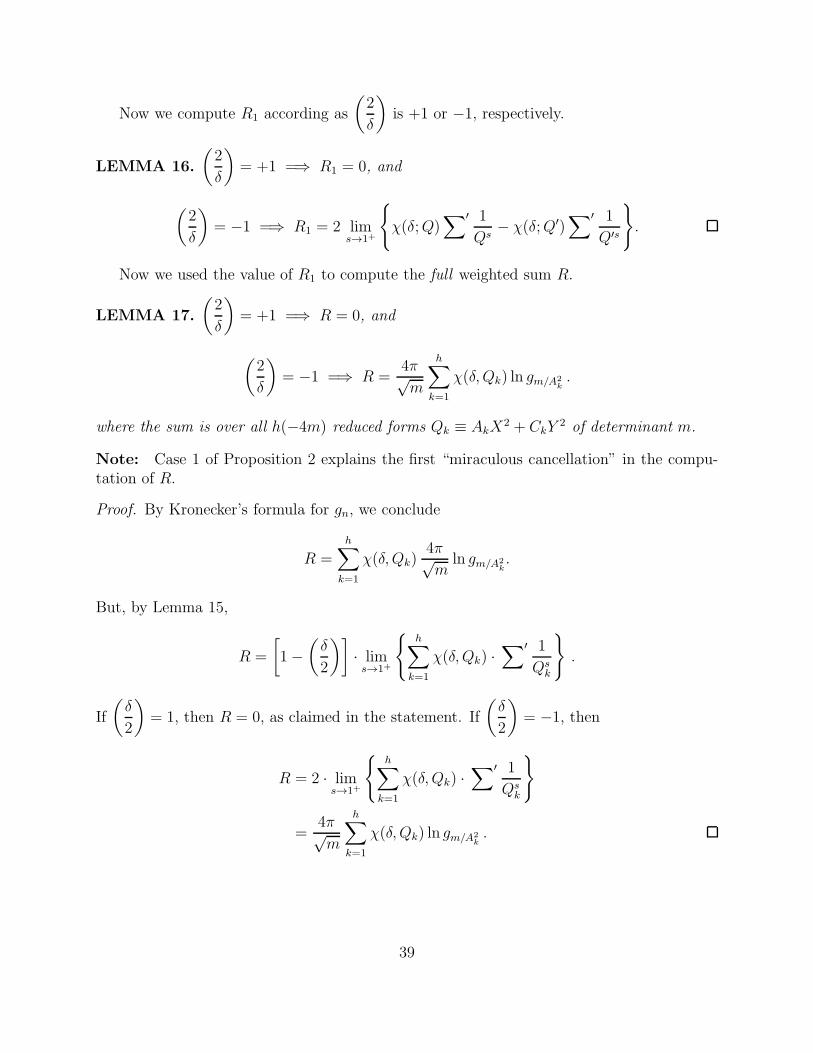
Now we compute R1 according as
(
2
δ
)
is +1 or −1, respectively.
LEMMA 16.
(
2
δ
)
= +1 =⇒ R1 = 0, and
(
2
δ
)
= −1 =⇒ R1 = 2 lims→1+
χ(δ;Q)∑′ 1
Qs− χ(δ;Q′)
∑′ 1
Q′s
.
Now we used the value of R1 to compute the full weighted sum R.
LEMMA 17.
(
2
δ
)
= +1 =⇒ R = 0, and
(
2
δ
)
= −1 =⇒ R =4π√m
h∑
k=1
χ(δ, Qk) ln gm/A2k.
where the sum is over all h(−4m) reduced forms Qk ≡ AkX2 + CkY
2 of determinant m.
Note: Case 1 of Proposition 2 explains the first “miraculous cancellation” in the compu-tation of R.
Proof. By Kronecker’s formula for gn, we conclude
R =
h∑
k=1
χ(δ, Qk)4π√m
ln gm/A2k.
But, by Lemma 15,
R =
[
1−(
δ
2
)]
· lims→1+
h∑
k=1
χ(δ, Qk) ·∑′ 1
Qsk
.
If
(
δ
2
)
= 1, then R = 0, as claimed in the statement. If
(
δ
2
)
= −1, then
R = 2 · lims→1+
h∑
k=1
χ(δ, Qk) ·∑′ 1
Qsk
=4π√m
h∑
k=1
χ(δ, Qk) ln gm/A2k.
39
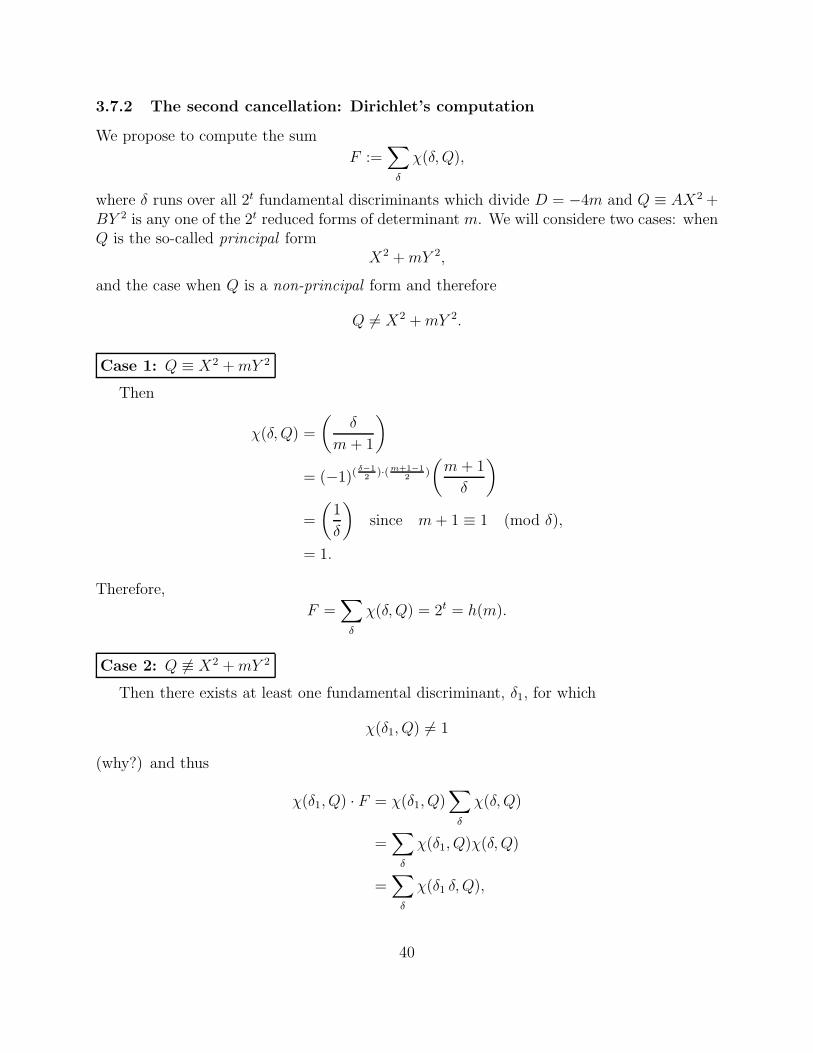
3.7.2 The second cancellation: Dirichlet’s computation
We propose to compute the sum
F :=∑
δ
χ(δ, Q),
where δ runs over all 2t fundamental discriminants which divide D = −4m and Q ≡ AX2 +BY 2 is any one of the 2t reduced forms of determinant m. We will considere two cases: whenQ is the so-called principal form
X2 +mY 2,
and the case when Q is a non-principal form and therefore
Q 6= X2 +mY 2.
Case 1: Q ≡ X2 +mY 2
Then
χ(δ, Q) =
(
δ
m+ 1
)
= (−1)(δ−1
2)·(m+1−1
2)
(
m+ 1
δ
)
=
(
1
δ
)
since m+ 1 ≡ 1 (mod δ),
= 1.
Therefore,
F =∑
δ
χ(δ, Q) = 2t = h(m).
Case 2: Q 6≡ X2 +mY 2
Then there exists at least one fundamental discriminant, δ1, for which
χ(δ1, Q) 6= 1
(why?) and thus
χ(δ1, Q) · F = χ(δ1, Q)∑
δ
χ(δ, Q)
=∑
δ
χ(δ1, Q)χ(δ, Q)
=∑
δ
χ(δ1 δ, Q),
40
where we have used the multiplicativity of the Jacobi symbol. Now comes the fundamen-tal observation (no pun intended!): As δ1 runs over the complete set of fundamental dis-
criminants dividing −4m, so does δ1 δ, and therefore the set of Jacobi symbols χ(δ1, Q)coincides with the set of Jacobi symbols χ(δ1 δ, Q). Therefore,
χ(δ1, Q) · F = F.
Butχ(δ1, Q) = −1,
or −F = F , i.e.,F = 0.
Written out,
F :=∑
δ
χ(δ, Q) = 0 for any Q 6= X2 +mY 2.
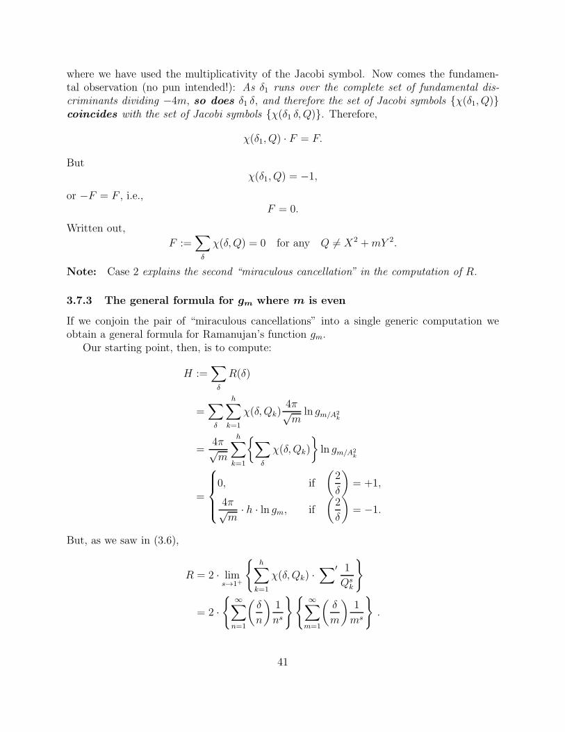
Note: Case 2 explains the second “miraculous cancellation” in the computation of R.
3.7.3 The general formula for gm where m is even
If we conjoin the pair of “miraculous cancellations” into a single generic computation weobtain a general formula for Ramanujan’s function gm.
Our starting point, then, is to compute:
H :=∑
δ
R(δ)
=∑
δ
h∑
k=1
χ(δ, Qk)4π√m
ln gm/A2k
=4π√m
h∑
k=1
∑
δ
χ(δ, Qk)
ln gm/A2k
=
0, if
(
2
δ
)
= +1,
4π√m
· h · ln gm, if
(
2
δ
)
= −1.
But, as we saw in (3.6),
R = 2 · lims→1+
h∑
k=1
χ(δ, Qk) ·∑′ 1
Qsk
= 2 · ∞∑
n=1
(
δ
n
)
1
ns
∞∑
m=1
(
δ
m
)
1
ms
.
41
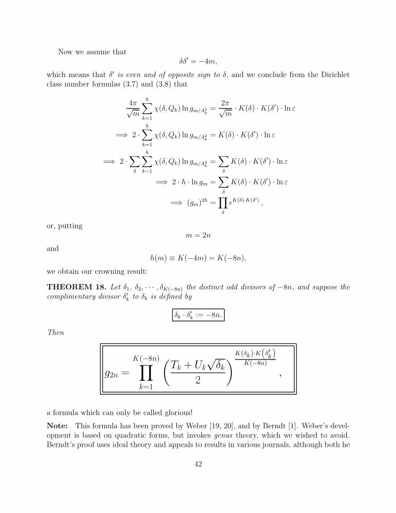
Now we assume thatδδ′ = −4m,
which means that δ′ is even and of opposite sign to δ, and we conclude from the Dirichletclass number formulas (3.7) and (3.8) that
4π√m
h∑
k=1
χ(δ, Qk) ln gm/A2k=
2π√m
·K(δ) ·K(δ′) · ln ε
=⇒ 2 ·h∑
k=1
χ(δ, Qk) ln gm/A2k= K(δ) ·K(δ′) · ln ε
=⇒ 2 ·∑
δ
h∑
k=1
χ(δ, Qk) ln gm/A2k=∑
δ
K(δ) ·K(δ′) · ln ε
=⇒ 2 · h · ln gm =∑
δ
K(δ) ·K(δ′) · ln ε
=⇒ (gm)2h =
∏
δ
ǫK(δ)·K(δ′) ,
or, puttingm = 2n
andh(m) ≡ K(−4m) = K(−8n),
we obtain our crowning result:
THEOREM 18. Let δ1, δ2, · · · , δK(−8n) the distinct odd divisors of −8n, and suppose the
complimentary divisor δ′k to δk is defined by
δk · δ′k := −8n.
Then
g2n =
K(−8n)∏
k=1
(
Tk + Uk
√δk
2
)
K(δk)·K(δ′k)K(−8n)
,
a formula which can only be called glorious!
Note: This formula has been proved by Weber [19, 20], and by Berndt [1]. Weber’s devel-opment is based on quadratic forms, but invokes genus theory, which we wished to avoid.Berndt’s proof uses ideal theory and appeals to results in various journals, although both he
42
and Weber obtain a more general result. Our development reveals the fundamental structureof all of these proofs without the extra baggage of (mathematically useful, but pedagogicallyobfuscatory) generalization.
This same formula can be used to compute g2n for all even convenient numbers which areof the form 2P where P is a product of distinct odd primes. In principle, this is just whatWeber did.
References
[1] Berndt, B. C., Ramanujan’s Notebooks, Part V, Springer, New York, 1998.
[2] Berndt, B. C., Chan, H. H., and Zhang, L.-C., “Ramanujan’s singular moduli,” The
Ramanujan Journal 1 (1997), 53–74.
[3] Borwein, J. M. and Borwein, P. B., π and the AGM, 2nd edition, Wiley, New York,1987.
[4] Chan, H. H., “Ramanujan’s class invariants and Watson’s empirical process,” J. LondonMath. Soc. (2), 57 (1998), 545–561.
[5] Chan, H. H. and Huang, S.-S., “On the Ramanujan–Golnitz–Gordon continued frac-tion,” The Ramanujan Journal 1 (1997), 75–90.
[6] Cox, D. A., Primes of the Form x2 +my2, 2nd edition, Wiley, New York, 1989.
[7] Euler, L., “Observationes de comparatione arcuum curvarum ellipticarum,” Novi
Commentarii Scientiarum Petropolitanae 6 (1761), 58–84; Opera Omnia ser. I, 20(Birkhauser, Basel, 1912), 80–107.
[8] Euler, L., “Extrait d’un lettre de M. Euler a M. Beguelin en Mai 1776,” Nouv. Mem.
Acad. Roy. Sci. Berlin (1776), 337–339.
[9] Fagnano, G., “Metodo per misurare la lemniscata,” Giorn. lett. d’Italia 29, 258.Reprinted in Opere matematiche, vol. 2, papers 32, 22, and 34, Allerighi e Segati,Milano, 1911.
[10] Flath, E. E., Introduction to Number Theory, Wiley, New York, 1989.
[11] Gauss, C. F., Disquisitiones Arithmeticae (translated by Arthur A. Clarke), Springer,New York, 1996.
[12] Greenhill, A. G., The Applications of Elliptic Functions, Dover, New York, 1959.
[13] Hardy, G. H., Ramanujan, Chelsea, New York, 1989.
[14] Jacobi, C. G. J., Fundamenta nova theoriae functionarum ellipticarum, Borntrager,Konigsberg, 1829. Reprinted in Gesammelte Werke, vol. 1, 49–239.
43
[15] Landen, J., “An investigation of a general theorem for finding the length of any arcof any conic hyperbola, by means of two elliptic arcs, with some other new and usefultheorems deduced therefrom,” Philos. Trans. Royal Soc. London 65 (1778), 283–289.
[16] Niven, N. and Zuckerman, H., An Introduction to the Theory of Numbers, 2nd edi-tion, Wiley, New York, 1966.
[17] Ramanujan, S., Collected Papers of Srinivasa Ramanujan, G. H. Hardy, P. V. SeshuAiyar, and B. M. Wilson, eds., Chelsea, New York, 1962.
[18] Watson, G. N., “Theorems stated by Ramanujan (XV): A singular modulus,” J. Lon-
don Math Soc. 46 (1931), 65–70.
[19] Weber, H., Lehrbuch der Algebra, Vol. III, 3rd edition, Chelsea, New York, 1961.
[20] Weber, H., “Zur complex Multiplikation elliptischer Functionen,” Math. Ann. 30(1887), 390–410.
[21] Weinberger, P. J., “Exponents of the class groups of complex quadratic fields,” Acta
Arith. 22 (1973), 117–124.
Received January 5, 2018MARK B. VILLARINO
Escuela de Matematica,Universidad de Costa Rica,2060 San Jose, Costa [email protected]
44